Exergetic Port-Hamiltonian Systems
for Multibody Dynamics

Abstract

Multibody dynamics simulation plays an important role in various fields, including mechanical engineering, robotics, and biomechanics. Setting up computational models however becomes increasingly challenging as systems grow in size and complexity. Especially the consistent combination of models across different physical domains usually demands a lot of attention. This motivates us to study formal languages for compositional modeling of multiphysical systems. This article shows how multibody systems, or more precisely assemblies of rigid bodies connected by lower kinematic pairs, fit into the framework of Exergetic Port-Hamiltonian Systems (EPHS). This approach is based on the hierarchical decomposition of systems into their ultimately primitive components, using a simple graphical syntax. Thereby, cognitive load can be reduced and communication is facilitated, even with non-experts. Moreover, the encapsulation and reuse of subsystems promotes efficient model development and management. In contrast to established modeling languages such as Modelica, the primitive components of EPHS are not defined by arbitrary equations. Instead, there are four kinds of components, each defined by a particular geometric structure with a clear physical interpretation. This higher-level approach could make the process of building and maintaining large-scale models simpler and also safer.

1 Introduction

1.1 EPHS modeling language

Exergetic Port-Hamiltonian Systems (EPHS), as recently formalized in [1], provide a compositional modeling language for physical systems. Specifically, the language is designed for the efficient combination of dynamic models from classical mechanics, electromagnetism, and irreversible processes (with local thermodynamic equilibrium).

The central paradigm is that systems are in general systems of systems. In other words, a model of a physical system is often best understood as an interconnection of simpler models. To make this intuitive, a graphical syntax is used to define interconnections. An expression in the EPHS syntax is hence called an interconnection pattern. Figure 1 shows an example. The round inner boxes of such formal diagrams correspond to (interfaces of) subsystems, while the rectangular outer box represents the interface of the composite system. The black dots are called junctions and the connected lines are called ports. An important feature of the language is that each junction corresponds to an energy domain, such as the potential or the kinetic energy domain (of a rigid body). Since ports expose energy domains, the mantra of EPHS is that systems are interconnected by sharing energy domains. This is reflected on the level of a single interconnection pattern and also by the fact that there is a unique way to flatten any hierarchy of nested interconnection patterns. Two interconnection patterns compose, i.e. they can be nested, whenever the outer interface of one pattern represents the same interface as some inner box of the other pattern. The syntax hence provides a graphical abstraction for dealing with interconnected and hierarchically nested systems in terms of their interfaces.

Any system is either a primitive system or a composite system (whose subsystems can be primitive or composite systems). There are different kinds of primitive systems representing either energy storage, reversible energy exchange or irreversible energy exchange. The semantics of a primitive system is accordingly determined by a geometric object, whose structure reflects the fundamental thermodynamic behavior. The semantics of a composite system is determined by the semantics of its subsystems and their interconnection. The interconnection is given by the respective interconnection pattern with each junction implying shared state and a power balance. Due to the structural properties of primitive systems and interconnections, all systems conform with the first and second law of thermodynamics, Onsager reciprocal relations, and some further conservation laws (e.g. for mass). Besides ensuring thermodynamic consistency, restricting the set of possible models in this way is a key enabling factor for their easy reusability.

1.2 Related work

The relationship between the EPHS modeling language, bond graph modeling, port-Hamiltonian systems, and the GENERIC formalism is already discussed in [1].

The presented approach to expressing multibody systems is closely related to the work of Sonneville and Brüls [2, 3], in the sense that essentially the same variables and constraints are used. The EPHS approach makes explicit the tearing and interconnection, based on which systems can be efficiently expressed. While it might seem irrelevant for multibody systems as such, the structural properties of EPHS demand that mechanical friction in the joint is modeled in a thermodynamically consistent way, making it straightforward to include thermal dynamics.

To a somewhat lesser extent, our approach is related to previous work on the port-Hamiltonian modeling of multibody systems [4, 5].

We demonstrate that our EPHS models agree with equations obtained from a suitable first principle from mechanics. Specifically, we use the Lagrange-d’Alembert-Pontryagin principle for implicit Lagrangian systems with constraints and external forces [6]. Since our models use velocity variables that are expressed in a body-fixed reference frame, we use the left-trivialized version of the principle, see [7]. Moreover, to model body and joint as separate subsystems, we use the tearing and interconnection approach for implicit Dirac-Lagrange systems [8]. Finally, to match the thermodynamically consistent description of mechanical friction, we use a constraint of thermodynamic type [9, 10].

1.3 Outline

Section 2 provides an introduction to the EPHS language and it introduces the proposed multibody framework in terms of interconnection patterns for the body model, the joint model, and a basic multibody system. Section 3 provides an introduction to the geometric description of multibody systems. Section 4 completes the definition of the body model by specifying the involved primitive subsystems, while Section 5 does the same for the joint model. For both models, it is shown that the resulting evolution equations agree with the Lagrange-d’Alembert-Pontryagin principle for interconnected implicit Lagrangian systems (with a constraint of thermodynamic type). Section 6 shows the system of differential-algebraic equations resulting from the interconnected EPHS and variational models. Section 7 concludes with a discussion of the results and possible directions for further research.

2 EPHS modeling language by example

With a detailed and formally precise introduction being available in [1], here we aim for a brief example-driven introduction. We start with an analogy. The essence of functional programming is function composition. Complex functions are implemented in terms of simpler functions, which again are composed of yet simpler functions. The functions on the lowest level are primitives provided by the execution environment. Analogously, the essence of EPHS is system interconnection. Complex systems are specified in terms of simpler systems, which themselves are composite systems. On the lowest level, primitive systems are defined by geometric objects that represent primitive physical behaviors, namely energy storage and reversible/irreversible energy exchange.

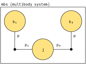
Figure 1: Interconnection pattern for a basic multibody system consisting of two bodies $\mathtt{b_{1}}$ and $\mathtt{b_{2}}$ connected by a joint $\mathtt{j}$.

While a graphical syntax for function composition is directed (similar to block diagrams), the EPHS syntax is undirected. Rather than feeding outputs to inputs, it expresses how various systems share energy domains. For instance, the pattern shown in Figure 1 defines a composite system in terms of three given subsystems. The name $\mathtt{mbs}$ is analogous to a function name, while $\mathtt{b_{1}}$, $\mathtt{b_{2}}$ and $\mathtt{j}$ are analogous to argument names. Specifically, boxes $\mathtt{b_{1}}$ and $\mathtt{b_{2}}$ represent two rigid bodies and $\mathtt{j}$ represents a joint that connects them. At this level, extending the multibody system to include more bodies and joints becomes conceptually very simple. The labor essentially reduces to setting the parameters associated to the subsystems in a meaningful way. The lines emanating from the inner boxes are inner ports which expose energy domains of the subsystems. Here, the ports $\mathtt{b_{1}.p}$ and $\mathtt{b_{2}.p}$ expose the kinetic energy domain of the two bodies. These energy domains are shared with the joint system $\mathtt{j}$, which essentially applies constraint forces such that the joint kinematics are satisfied. The rectangular outer box represents the interface of the composite system. Here, there are no outer ports, so the composite system is isolated.

The round inner boxes as well as the outer box represent interfaces, which are collections of ports. Although not shown in the graphical representation, next to its name, each port is defined by a physical quantity, which is the quantity that can be exchanged via the port. In Figure 1 all ports belong to a kinetic energy domain, so momentum is the exchanged physical quantity. All quantities have an associated space of values. This extra data ensures that interconnections are well typed. In summary, each box represents the interface of a system. An interface is given by a collection of ports with associated quantities. Each port exposes an energy domain of the system to which it belongs. Whenever two ports are connected at a junction, the respective systems may share information about the current value of the respective quantity and they may exchange energy by exchanging the respective quantity.

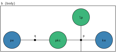
Figure 2: Interconnection pattern for the rigid body model. Box $\mathtt{pe}$ represents storage of potential energy, while box $\mathtt{ke}$ represents storage of kinetic energy. Box $\mathtt{pkc}$ represents the reversible coupling of the potential and kinetic energy domains. Box $\mathtt{lp}$ represents the gyroscopic effects (Lie-Poisson structure).

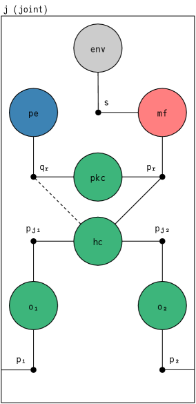
Figure 3: Interconnection pattern for the joint model. Box $\mathtt{hc}$ represents the holonomic constraint describing the joint kinematics. Boxes $\mathtt{o_{1}}$ and $\mathtt{o_{2}}$ take into account the offset between the reference frame of one of the connected bodies and the reference frame defining the respective joint force application point. Box $\mathtt{pe}$ represents a possible storage of potential energy, depending on the relative pose of the two connected bodies. Box $\mathtt{pkc}$ represents the coupling between the potential and kinetic energy domains of the joint. Box $\mathtt{mf}$ represents the irreversible process of mechanical friction and box $\mathtt{env}$ represents the environment which directly absorbs the generated heat.

The yellow color of the inner boxes in Figure 1 is an annotation indicating that the body and joint subsystems are again composite systems and therefore defined via separate interconnection patterns. The patterns for the body and joint models are shown in Figures 2 and 3, respectively. It is important to note that the hierarchical nesting of systems is defined since the interface represented by the outer box of the body/joint pattern is equivalent (up to a renaming of ports) to the interface represented by the respective inner boxes in Figure 1. To illustrate this, the flattened pattern is shown explicitly in Figure 4. Based on this uniquely defined notion of composition, systems can be easily and safely decomposed (or refactored) into manageable and reusable parts.

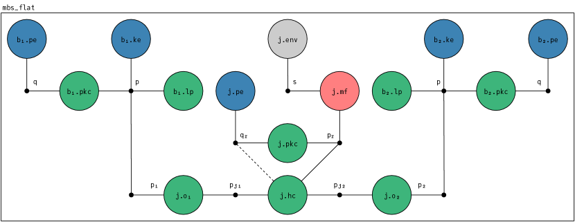
Figure 4: Flattened interconnection pattern for the basic multibody system. The pattern is obtained by substituting the pattern in Figure 2 into the inner boxes $\mathtt{b_{1}}$ and $\mathtt{b_{2}}$ of the pattern in Figure 1 and further by substituting the pattern in Figure 3 into the inner box $\mathtt{j}$.

We briefly remark that there are two kinds of ports. The dashed line in Figure 3 represents a state port, rather than a power port. A state port may exchange information about the state of the respective quantity, while a power port additionally allows for energy exchange.

We also remark that we use an abbreviated notation to write down the port names when visualizing interconnection patterns. Whenever multiple ports connected to the same junction have the same name, we write the name only once at the junction.

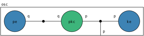
Figure 5: Interconnection pattern for a mechanical oscillator model. Box $\mathtt{pe}$ represents storage of potential energy. Box $\mathtt{ke}$ represents storage of kinetic energy. Box $\mathtt{pkc}$ represents the reversible coupling between the potential energy domain, represented by the junction on its left, and the kinetic energy domain represented by the junction on its right. The outer port $\mathtt{p}$ exposes the kinetic energy domain.

To go into more detail, we now turn our attention to the simplest example, namely that of a 1D mechanical oscillator, which is defined using the interconnection pattern shown in Figure 5. The pattern is similar to that of the rigid body model, except there is no subsystem for gyroscopic effects. Moreover, the interfaces of the equally-named subsystems are not equivalent, since the quantities of the corresponding ports have different underlying spaces. Here, they are just $1$-dimensional. Next, we define the three primitive subsystems including their interfaces and then we come back to the interconnection pattern and show how the three systems are combined according to it.

When we define interfaces, we need to choose quantities for the ports form a set of possible quantities $\mathbf{Q}$. Rather than defining this set upfront, we simply state the relevant elements (quantities) as we go. Besides that, systems are defined with respect to an exergy reference environment, which enables the thermodynamically consistent combination of reversible and irreversible dynamics. For the purposes of this paper, it is sufficient to define the absolute environment temperature ${\color[rgb]{.5,0,.5}\theta}$.

We now define the first primitive system, namely the storage component $(I_{\text{pe}},\,E_{\text{pe}})$ filling the box $\mathtt{pe}$. Its interface $I_{\text{pe}}=(\{\mathtt{q}\},\,\tau_{\text{pe}})$ is defined by the set of ports $\{\mathtt{q}\}$ and a function $\tau_{\text{pe}}:\{\mathtt{q}\}\rightarrow\mathbf{Q}\times\{\mathsf{p},\,\mathsf{s}\}$ that assigns to each port its quantity as well as a Boolean value indicating whether the port is a power or a state port. Here, we have $\tau_{\text{pe}}(\mathtt{q})=((\mathbb{R},\,\mathtt{displacement}),\,\mathsf{p})$, where $(\mathbb{R},\,\mathtt{displacement})\in\mathbf{Q}$ represents the quantity displacement with underlying state space $\mathbb{R}$, while the choice $\mathsf{p}\in\{\mathsf{p},\,\mathsf{s}\}$ indicates that $\mathtt{q}$ is a power port. The state space $\mathcal{X}_{I}$ associated to an interface $I$ is the Cartesian product of the state spaces of its ports. Here, we simply have $\mathcal{X}_{I_{\text{pe}}}=\mathbb{R}$. Next to its interface, a storage component is defined by an energy function, which assigns to each state the corresponding stored energy. Here, we assume a Hookean spring. Hence, the function $E_{\text{pe}}:\mathcal{X}_{I_{\text{pe}}}\rightarrow\mathbb{R}$ is defined by $E_{\text{pe}}(q)=\frac{1}{2}\,k\,q^{2}$, where $q\in\mathcal{X}_{I_{\text{pe}}}$ denotes the displacement and $k\in\mathbb{R}$ is a parameter of the model (stiffness).

All ports have a state variable $\mathtt{x}$, while power ports additionally have a flow variable $\mathtt{f}$ and an effort variable $\mathtt{e}$. For the power port $\mathtt{q}$, we have the port variables $(\mathtt{q.x},\,\mathtt{q.f},\,\mathtt{q.e})\in\mathrm{T}\mathcal{X}_{\mathtt{q}}\oplus\mathrm{T}^{*}\mathcal{X}_{\mathtt{q}}$, where $\mathcal{X}_{\mathtt{q}}=\mathbb{R}$ is the state space of the port and $\mathrm{T}\mathcal{X}_{\mathtt{q}}\oplus\mathrm{T}^{*}\mathcal{X}_{\mathtt{q}}$ denotes the Whitney sum of the tangent bundle and cotangent bundle over $\mathcal{X}_{\mathtt{q}}$. These geometric concepts are briefly discussed in Section 3. In this case, we can simply identify $\mathrm{T}\mathcal{X}_{\mathtt{q}}\oplus\mathrm{T}^{*}\mathcal{X}_{\mathtt{q}}\cong\mathbb{R}\times\mathbb{R}\times\mathbb{R}$. All port variables of an interface together form a vector bundle. Based on this, the semantics of interconnection patterns, primitive systems, and composite systems can be understood geometrically within a simple framework based on relations between such bundles and the composition of these relations [1]. Here, we discuss semantics in terms of equations only.

The semantics of the storage component $(I_{\text{pe}},\,E_{\text{pe}})$ filling the box $\mathtt{pe}$ is given by

$$\begin{split}\mathtt{pe.q.x}\>&=\>q\\ \mathtt{pe.q.f}\>&=\>\dot{q}\\ \mathtt{pe.q.e}\>&=\>\differential E_{\text{pe}}(q)\>=\>k\,q\,.\end{split}$$ (1)

The flow variable is the rate of change of the state variable (velocity) and the effort variable is the differential of the stored energy at the current state (force). The duality pairing $\langle\mathtt{q.e}\mid\mathtt{q.f}\rangle=\langle\differential E_{\text{pe}}(q)\mid\dot{q}\rangle=k\,q\,\dot{q}$ is the power supplied to the system. The concepts of differential and linear duality are discussed in Section 3. With the identification $\mathrm{T}\mathcal{X}_{\mathtt{q}}\oplus\mathrm{T}^{*}\mathcal{X}_{\mathtt{q}}\cong\mathbb{R}\times\mathbb{R}\times\mathbb{R}$, the duality pairing simply becomes scalar multiplication.

We also remark that in general the effort variables are given by the differential of an exergy function that is induced from the energy function based on the reference environment. Since all storage components in this paper store forms of mechanical energy, the respective exergy and energy functions are equal.

The storage component $(I_{\text{ke}},\,E_{\text{ke}})$ filling the box $\mathtt{ke}$ is defined by its interface $I_{\text{ke}}=(\{\mathtt{p}\},\,\tau_{\text{ke}})$ with $\tau_{\text{ke}}(\mathtt{p})=((\mathbb{R},\,\mathtt{momentum}),\,\mathsf{p})$ and its energy function $E_{\text{ke}}:\mathcal{X}_{I_{\text{ke}}}\rightarrow\mathbb{R}$ given by $E_{\text{ke}}(p)=\frac{1}{2\,m}\,p^{2}$, where $p\in\mathcal{X}_{I_{\text{ke}}}=\mathbb{R}$ denotes the momentum and $m\in\mathbb{R}$ is a parameter of the model (mass). The semantics is hence given by

$$\begin{split}\mathtt{ke.p.x}\>&=\>p\\ \mathtt{ke.p.f}\>&=\>\dot{p}\\ \mathtt{ke.p.e}\>&=\>\differential E_{\text{ke}}(p)\>=\>\frac{1}{m}\,p\,.\end{split}$$ (2)

The reversible component $(I_{\text{pkc}},\,\mathcal{D}_{\text{pkc}})$ filling the box $\mathtt{pkc}$ is defined by its interface $I_{\text{pkc}}=(\{\mathtt{q},\,\mathtt{p}\},\,\tau_{\text{pkc}})$ with $\tau_{\text{pkc}}(\mathtt{q})=((\mathbb{R},\,\mathtt{displacement}),\,\mathsf{p})$ as well as $\tau_{\text{pkc}}(\mathtt{p})=((\mathbb{R},\,\mathtt{momentum}),\,\mathsf{p})$ and its Dirac structure $\mathcal{D}_{\text{pkc}}$, which defines the semantics given by

$$\left[\begin{array}[]{c}\mathtt{pkc.q.f}\\ \mathtt{pkc.p.f}\end{array}\right]\>=\>\left[\begin{array}[]{rrr}0&-1\\ 1&0\end{array}\right]\,\left[\begin{array}[]{c}\mathtt{pkc.q.e}\\ \mathtt{pkc.p.e}\end{array}\right]\,.$$ (3)

We note that the skew-symmetric matrix used to represent a Dirac structure implies conservation of power. Here, we have $\langle\mathtt{q.e}\mid\mathtt{q.f}\rangle+\langle\mathtt{p.e}\mid\mathtt{p.f}\rangle=0$.

Coming back to the interconnection pattern in Figure 5, the semantics is given junction by junction. We have

$$\mathtt{pe.q.x}\>{}={}\> \mathtt{pkc.q.x}$$ (4a)

$$\mathtt{pe.q.f}\>{}+{}\> \mathtt{pkc.q.f}\>{}={}\>0$$

$$\mathtt{pe.q.e}\>{}={}\> \mathtt{pkc.q.e}$$

and

$$\mathtt{pkc.p.x}\>{}={}\> \mathtt{ke.p.x}\>{}={}\>\mathtt{p.x}$$ (4b)

$$\mathtt{pkc.p.f}\>{}+{}\> \mathtt{ke.p.f}\>{}={}\>\mathtt{p.f}$$

$$\mathtt{pkc.p.e}\>{}={}\> \mathtt{ke.p.e}\>{}={}\>\mathtt{p.e}\,.$$

In general, at every junction the state variables of all connected ports are equal. Further, the sum of the flow variables of all connected inner power ports is equal to the sum of the flow variables of all connected outer power ports. Finally, the effort variables of all connected power ports are equal. By eliminating interface variables, Equations 1, 2, 3 and 4b can be reduced to

$$\begin{split}\dot{q}\>&=\>\frac{1}{m}\,p\>=\>\mathtt{p.e}\\ \dot{p}\>&=\>-k\,q\,+\,\mathtt{p.f}\,.\end{split}$$ (5)

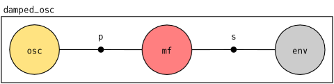
Figure 6: Interconnection pattern for a damped oscillator model. Box $\mathtt{osc}$ represents the mechanical oscillator model defined based on the pattern in Figure 5. Box $\mathtt{mf}$ represents mechanical friction and box $\mathtt{env}$ represents the environment, which absorbs the generated heat.

To add an irreversible process to the system, we regard it as a subsystem filling the inner box $\mathtt{osc}$ of the interconnection pattern shown in Figure 6. Next we define the two additional components.

The irreversible component $(I_{\text{mf}},\,\mathcal{O}_{\text{mf}})$ filling the box $\mathtt{mf}$ is defined by its interface $I_{\text{mf}}=(\{\mathtt{p},\,\mathtt{s}\},\,\tau_{\text{mf}})$ with $\tau_{\text{mf}}(\mathtt{p})=((\mathbb{R},\,\mathtt{momentum}),\,\mathsf{p})$, $\tau_{\text{mf}}(\mathtt{s})=((\mathbb{R},\,\mathtt{entropy}),\,\mathsf{p})$ and its Onsager structure $\mathcal{O}_{\text{mf}}$, which defines the semantics given by

$$\begin{bmatrix}\mathtt{mf.p.f}\\ \mathtt{mf.s.f}\end{bmatrix}\>=\>\frac{1}{{\color[rgb]{.5,0,.5}\theta_{0}}}\,d\,\begin{bmatrix}\theta&-\upsilon\\ -\upsilon&\frac{\upsilon^{2}}{\theta}\end{bmatrix}\,\begin{bmatrix}\mathtt{mf.p.e}\\ \mathtt{mf.s.e}\end{bmatrix}\>=\>\begin{bmatrix}d\,\upsilon\\ -\frac{1}{\theta}\,d\,\upsilon^{2}\end{bmatrix}\,.$$ (6)

Here, $\upsilon=\mathtt{p.e}$ is the velocity and $\theta={\color[rgb]{.5,0,.5}\theta_{0}}+\mathtt{s.e}$ is the absolute temperature at which kinetic energy is dissipated into the thermal energy domain. These variables can be interpreted as thermodynamic driving forces. Further, $d\in\mathbb{R}$ is a parameter (friction coefficient). The flow variable $\mathtt{p.f}$ is the friction force and $\mathtt{s.f}$ is the entropy production rate, with an additional minus sign, since entropy leaves the system. These variables can be interpreted as the resulting thermodynamic fluxes. The symmetric non-negative definite matrix used to define the Onsager structure implies non-negative exergy destruction, which is equivalent to non-negative entropy production. Specifically, the exergy destruction rate is $\langle\mathtt{p.e}\mid\mathtt{p.f}\rangle+\langle\mathtt{s.e}\mid\mathtt{s.f}\rangle={\color[rgb]{.5,0,.5}\theta_{0}}\,\frac{1}{\theta}\,d\,\upsilon^{2}$, where $\frac{1}{\theta}\,d\,\upsilon^{2}$ is the entropy production rate. Energy is conserved since (see [1] for details)

$$\begin{bmatrix}\theta&-\upsilon\\ -\upsilon&\frac{\upsilon^{2}}{\theta}\end{bmatrix}\,\begin{bmatrix}\upsilon\\ \theta\end{bmatrix}\>=\>\begin{bmatrix}0\\ 0\end{bmatrix}\,.$$

We note that the Dirac/Onsager structures of reversible/irreversible components in general have to satisfy further properties to ensure thermodynamic consistency [1].

The environment component essentially is a storage component that represents the thermal energy domain of the isothermal reference environment. By definition, its exergy function always takes the value zero. Hence, the effort variable is also zero. Its semantics is then given by

$$\begin{split}\mathtt{env.s.x}\>&=\>s\\ \mathtt{env.s.f}\>&=\>\dot{s}\\ \mathtt{env.s.e}\>&=\>0\,.\end{split}$$ (7)

By eliminating interface variables, Equations 5, 6 and 7 combined with those for the pattern in Figure 6 can be reduced to

$$\begin{split}\dot{q}\>&=\>\upsilon\\ \dot{p}\>&=\>-k\,q-d\,\upsilon\\ \dot{s}\>&=\>\frac{1}{\theta_{0}}\,d\,\upsilon^{2}\,,\end{split}$$ (8)

where $\upsilon=\frac{1}{m}\,p$.

We may say that the semantics of EPHS is functorial since Equation 8 can be equally obtained by first substituting the pattern in Figure 5 into the pattern in Figure 6, which gives the pattern in Figure 7, and then filling its inner boxes with the same components. Hence, the composition of interconnection patterns (syntax) is indeed compatible with interconnecting systems (semantics).

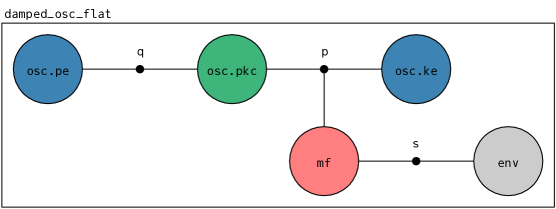
Figure 7: Interconnection pattern of the rigid body model.

3 Geometric foundation

Here, we aim for a brief introduction to the geometric concepts used in this paper. More details can be found in textbooks such as [11] or [12, 13].

3.1 Physical space and coordinate frames

The Euclidean vector space $(\mathbb{E}^{3},\,\langle\cdot\ ,\,\cdot\rangle)$ is a real $3$-dimensional vector space $\mathbb{E}^{3}$ with an inner product $\langle\cdot\ ,\,\cdot\rangle:\mathbb{E}^{3}\times\mathbb{E}^{3}\rightarrow\mathbb{R}$.

A choice of orthonormal basis for $\mathbb{E}^{3}$ gives an isomorphism $\mathbb{E}^{3}\cong\mathbb{R}^{3}$. The orthonormality condition ensures that the isomorphism preserves the inner product, with the inner product of $\mathbb{R}^{3}$ being the dot product. Specifically, let’s consider two right-handed orthonormal bases $(e_{1}^{I},\,e_{2}^{I},\,e_{3}^{I})$ and $(e_{1}^{B},\,e_{2}^{B},\,e_{3}^{B})$. A vector $v\in\mathbb{E}^{3}$ can then be represented as

$$v\>=\>{}_{I}v^{1}\,e_{1}^{I}+{}_{I}v^{2}\,e_{2}^{I}+{}_{I}v^{3}\,e_{3}^{I}\>=\>{}_{B}v^{1}\,e_{1}^{B}+{}_{B}v^{2}\,e_{2}^{B}+{}_{B}v^{3}\,e_{3}^{B}\,,$$

where ${}_{I}v=({}_{I}v^{1},\,{}_{I}v^{2},\,{}_{I}v^{3})\in\mathbb{R}^{3}$ is the coordinate representation of $v$ with respect to basis $I$ and ${}_{B}v=({}_{B}v^{1},\,{}_{B}v^{2},\,{}_{B}v^{3})\in\mathbb{R}^{3}$ is its representation with respect to basis $B$. For computations in coordinates, we regard these as column vectors, i.e. we identify $\mathbb{R}^{3}\cong\mathbb{R}^{3\times 1}$, and we simply use juxtaposition to denote matrix multiplication. For instance, we have $\langle v,\,v\rangle={}_{I}v^{\mathrm{T}}{}_{I}v={}_{B}v^{\mathrm{T}}{}_{B}v$, since $I$ and $B$ are orthonormal.

The two representations are related by

$${}_{I}v\>=\>R_{IB}\,{}_{B}v\,,$$

where the coordinate transformation matrix $R_{IB}\in\mathbb{R}^{3\times 3}$ contains the basis vectors of $B$ expressed in the basis $I$, i.e. $R_{IB}=\bigl{[}{}_{I}e_{1}^{B}\ \mid{}_{I}e_{2}^{B}\ \mid{}_{I}e_{3}^{B}\bigr{]}$. With $E\in\mathbb{R}^{3\times 3}$ denoting the identity matrix, we have $R_{IB}^{\mathrm{T}}\,R_{IB}=R_{BI}\,R_{IB}=E$, since the transformation preserves the inner product, and moreover we have $\det(R_{IB})=1$, as it also preserves the right-handed orientation. $R_{IB}$ is commonly called a rotation matrix.

The Euclidian (affine) space $(\mathcal{E}^{3},\,+)$ with associated vector space $\mathbb{E}^{3}$ shall represent physical space. By definition, for any two points $P,\,Q\in\mathcal{E}^{3}$, there is a unique vector denoted by $r_{PQ}\in\mathbb{E}^{3}$ that represents the translation from $P$ to $Q$. So, the vector space $\mathbb{E}^{3}$ acts (transitively) on the point space $\mathcal{E}^{3}$ by translation and we have $P+r_{PQ}=Q$, where $+:\mathcal{E}^{3}\times\mathbb{E}^{3}\rightarrow\mathcal{E}^{3}$ denotes the (affine) action.

A coordinate frame $(A,\,(e_{1}^{A},\,e_{2}^{A},\,e_{3}^{A}))$ is defined by an origin $A\in\mathcal{E}^{3}$ and a basis for $\mathbb{E}^{3}$. Hence, a frame gives an isomorphism $\mathcal{E}^{3}\cong\mathbb{R}^{3}$. We reuse the same symbol, here $A$, to refer to a frame or just to its origin or its basis. In particular, we use $I$ to denote the inertial reference frame $(I,\,(e_{1}^{I},\,e_{2}^{I},\,e_{3}^{I}))$ used throughout.

3.2 Configuration of a rigid body

At rest, a rigid body $(\mathcal{B},\,\rho)$ is characterized by its set of material points (reference configuration) $\mathcal{B}\subset\mathcal{E}^{3}$ and its mass density function $\rho:\mathcal{B}\rightarrow\mathbb{R}_{+}$. Let $(B,\,(e_{1}^{B},\,e_{2}^{B},\,e_{3}^{B}))$ be a frame with origin $B\in\mathcal{B}$. Considering the possibility of motion, we say that $B$ is a body-fixed frame when it moves with the body. Assuming this, the time-dependent position of an arbitrary particle $P\in\mathcal{B}$ with respect to the reference frame $I$ can be written as

$${}_{I}r_{IP}(t)\>=\>{}_{I}r_{IB}(t)+R_{IB}(t)\,{}_{B}r_{BP}\,,$$ (9)

where ${}_{B}r_{BP}\in\mathbb{R}^{3}$ is constant due to the body’s rigidity. Hence, the time-dependent configuration of the rigid body is given by

$$q_{IB}(t)\>=\>\bigl{(}R_{IB}(t),\,{}_{I}r_{IB}(t)\bigr{)}\>\in\>\mathrm{SO}(3)\times\mathbb{R}^{3}\,.$$ (10)

We also say that $q_{IB}(t)$ is the absolute pose of the body, as it is given relative to the distinguished reference frame $I$. The set of matrices

$$\mathrm{SO}(3)\>=\>\Bigl{\{}R\in\mathbb{R}^{3\times 3}\,\mid\,R^{\mathrm{T}}R=E\>;\>\det(R)=1\Bigr{\}}$$

forms a matrix Lie group, as it forms a smooth $3$-dimensional space (manifold) as well as a group, with the composition operation (matrix multiplication) and the inverse operation (matrix transposition) being smooth maps. $\mathrm{SO}(3)$ is called special orthogonal group or simply rotation group.

3.3 Lie group structure of the configuration space

The Lie group structure of the space of all possible configurations, gives rise to mathematical operations that are central to the description of rigid-body dynamics.

Next to $\mathrm{SO}(3)$, also $\mathbb{R}^{3}$ is a Lie group, since vector spaces are Lie groups, with the composition operation being vector addition and the inverse operation being scalar multiplication by $-1$. The configuration space $\mathrm{SO}(3)\times\mathbb{R}^{3}$ then also forms a Lie group, called the direct product.

Because $\mathrm{SO}(3)$ acts on $\mathbb{R}^{3}$ by matrix-vector multiplication, the configuration space admits yet another group structure, called the semidirect product. This group is denoted by $\mathrm{SO}(3)\ltimes\mathbb{R}^{3}=\mathrm{SE}(3)$ and it is also called the special Euclidian group.

Since both Lie groups can be used as a geometric basis for describing rigid body dynamics [14, 15], we use the symbol $G$ to denote either of the two. The composition operation $G\times G\rightarrow G$, which we denote simply by juxtaposition, is defined by

$$G=\mathrm{SO}(3)\times\mathbb{R}^{3}\colon (R_{1},\,r_{1})\,(R_{2},\,r_{2})\>=\>(R_{1}\,R_{2},\,r_{1}+r_{2})$$

$$G=\mathrm{SO}(3)\ltimes\mathbb{R}^{3}\colon (R_{1},\,r_{1})\,(R_{2},\,r_{2})\>=\>(R_{1}\,R_{2},\,r_{1}+{\color[rgb]{.5,0,.5}R_{1}}\,r_{2})\,.$$

In both cases, the identity element is $e=(E,\,0)\in G$. The inverse operation ${(\cdot)}^{-1}:G\rightarrow G$ is then defined by

$$G=\mathrm{SO}(3)\times\mathbb{R}^{3}\colon (R,\,r)^{-1}\>=\>(R^{\mathrm{T}},-r)$$

$$G=\mathrm{SO}(3)\ltimes\mathbb{R}^{3}\colon (R,\,r)^{-1}\>=\>(R^{\mathrm{T}},\,-{\color[rgb]{.5,0,.5}R^{\mathrm{T}}}\,r)\,.$$

3.4 Geometric interpretation of composition

The difference between the two group structures becomes apparent when the absolute pose $q_{IB}=(R_{IB},\,{}_{I}r_{IB})$, as defined by Equation 10, is composed with a relative pose $q_{BC}$, where $C$ is the origin of another frame $(C,\,(e_{1}^{C},\,e_{2}^{C},\,e_{3}^{C}))$. Let $q_{IC}=(R_{IC},\,{}_{I}r_{IC})$ denote the corresponding absolute pose. The relative pose $q_{BC}$ is then defined by $q_{IC}=q_{IB}\,q_{BC}$. As we show next, the different composition operations imply different definitions for $q_{BC}$.

The case $G=\mathrm{SO}(3)\times\mathbb{R}^{3}$ corresponds to the relative translation $r_{BC}$ being expressed in the inertial basis $I$, i.e. $q_{BC}=(R_{BC},\,{}_{I}r_{BC})$, since based on

$$q_{IC}\>=\>q_{IB}\,q_{BC}\>=\>(R_{IB},\,{}_{I}r_{IB})\,(R_{BC},\,{}_{I}r_{BC})\>=\>(R_{IB}\,R_{BC},\,{}_{I}r_{IB}+{}_{I}r_{BC})\,$$

we can write the position of an arbitrary particle $P\in\mathcal{B}$ as

$${}_{I}r_{IP} =\>{}_{I}r_{IC}+R_{IC}\,{}_{C}r_{CP}$$

$$=\>{\color[rgb]{.5,0,.5}{}_{I}r_{IB}+{}_{I}r_{BC}}+{\color[rgb]{.5,0,.5}R_{IB}\,R_{BC}}\,{}_{C}r_{CP}\,.$$

The case $G=\mathrm{SO}(3)\ltimes\mathbb{R}^{3}$, corresponds to the relative translation $r_{BC}$ being expressed in the basis $B$, i.e. $q_{BC}=(R_{BC},\,{}_{B}r_{BC})$, since based on

$$q_{IC}\>=\>q_{IB}\,q_{BC}\>=\>(R_{IB},\,{}_{I}r_{IB})\,(R_{BC},\,{}_{B}r_{BC})\>=\>(R_{IB}\,R_{BC},\,{}_{I}r_{IB}+R_{IB}\,{}_{B}r_{BC})\,$$

we can write the position of an arbitrary particle $P\in\mathcal{B}$ as

$${}_{I}r_{IP} =\>{}_{I}r_{IC}+R_{IC}\,{}_{C}r_{CP}$$

$$=\>{\color[rgb]{.5,0,.5}{}_{I}r_{IB}+R_{IB}\,{}_{B}r_{BC}}+{\color[rgb]{.5,0,.5}R_{IB}\,R_{BC}}\,{}_{C}r_{CP}\,.$$

3.5 Material velocity

According to Equation 9, the position of any particle $P\in\mathcal{B}$ can be written in terms of the configuration $q_{IB}(t)=\bigl{(}R_{IB}(t),\,{}_{I}r_{IB}(t)\bigr{)}\in G$ of the body $\mathcal{B}$, which is seen to be a smooth curve $q_{IB}:\mathbb{I}\to G$ with time interval $\mathbb{I}\subset\mathbb{R}$. Since ${}_{B}r_{BP}$ is constant, the velocity of the particle is given by

$${}_{I}\dot{r}_{IP}(t)\>=\>{}_{I}\dot{r}_{IB}(t)+\dot{R}_{IB}(t)\,{}_{B}r_{BP}\,,$$

which depends solely on the material velocity $\dot{q}_{IB}(t)=\bigl{(}\dot{R}_{IB}(t),\,{}_{I}\dot{r}_{IB}(t)\bigr{)}\in\mathrm{T}_{q_{IB}}G$. The vector space $\mathrm{T}_{q_{IB}}G$ of all possible velocities at configuration $q_{IB}$ is discussed next.

3.6 The derivative (interlude)

A smooth manifold $M$ has a notion of neighborhoods around points. By definition, for every neighborhood (open set) $U\subset M$, there is a smooth isomorphism $x\colon U\to x(U)$ that takes any point in $U$ to its coordinate representation in $x(U)\subseteq\mathbb{R}^{n}$, where $n=\dim(M)$. The smooth map $x$ is called a coordinate chart on $U$. While a single chart suffices for a flat space such as $\mathcal{E}^{3}$, in general it takes multiple overlapping charts to cover a manifold.

As the derivative is a local operator, it can be computed numerically on the chart level. Staying on the coordinate-free level, let $f:M\to N$ be any smooth function between two smooth manifolds. The derivative of $f$ evaluated at point $p\in M$ is the linear function

$$\begin{split}\mathrm{T}_{p}f\colon\mathrm{T}_{p}M&\to\mathrm{T}_{f(p)}N\\ v&\mapsto\derivative{t}\,\Big{|}_{t=0}\,f(c(t))\,,\end{split}$$

where $c:\mathbb{I}\to M$ with $\mathbb{R}\supseteq\mathbb{I}\ni 0$ is an arbitrary smooth curve on $M$ such that $c(0)=p$ and $\dot{c}(0)=v$. So, the derivative of a smooth curve $c$ at some point (in time, here $0$) is a vector $v\in\mathrm{T}_{c(0)}M$, which is seen to be tangent to the curve at that point. The tangent space over point $p$, denoted as $\mathrm{T}_{p}M$, is simply the vector space of all possible tangent vectors at $p$, considering all possible curves passing through $p$. Finally, the derivative $\mathrm{T}f$ of any smooth function $f$ is the linear function that propagates tangent vectors along $f$. Going one level up, the disjoint union of all tangent spaces $\mathrm{T}M=\sqcup_{p\in M}\mathrm{T}_{p}M$ forms again a smooth manifold, called the tangent bundle over $M$. We have $\dim(\mathrm{T}M)=2\cdot\dim(M)$, since for every point $p\in M$, there are $\dim(\mathrm{T}_{p}M)=\dim(M)$ directions for change. So, $\mathrm{T}$ sends a manifold $M$ to its tangent bundle $\mathrm{T}M$ and it sends a smooth map $f:M\to N$ between manifolds to its derivative $\mathrm{T}f:\mathrm{T}M\to\mathrm{T}N$. For any composite function $f=f_{2}\circ f_{1}$, it satisfies the chain rule (functor property) $\mathrm{T}f=\mathrm{T}f_{2}\circ\mathrm{T}f_{1}$.

We now connect this to the differential $\differential f$ of a function $f\colon M\to\mathbb{R}$, as used in Equations 1 and 2. First, we notice that for a function $f\colon M\to N$ between arbitrary manifolds, the derivative is a map $\mathrm{T}f\colon\mathrm{T}M\to\mathrm{T}N$ that sends any pair $(p,\,v)$ with $p\in M$ and $v\in\mathrm{T}_{p}M$ to the pair $(q,\,w)$ with $q=f(p)$ and $w\in\mathrm{T}_{q}N$ being the infinitesimal change of $f(p)$ when the local change of $p$ is given by $v$. To make composition work (chain rule), it is important to also propagate the local points such as $q$ and $p$ and not only the local changes $v$ and $w$. In contrast to the derivative, the differential is a concept that only applies to functions $f:M\to\mathbb{R}$ on manifolds. At point $p$, the differential $\differential f(p)$ does not include the value $f(p)$. It simply is a covector $\differential f(p)\in\mathrm{T}^{*}_{p}M$, i.e. a linear function that sends a vector $v\in\mathrm{T}_{p}M$ to the corresponding infinitesimal change $w\in\mathrm{T}_{f(p)}\mathbb{R}\cong\mathbb{R}$. We write $w=\langle\differential f(p)\mid v\rangle$ for the duality pairing. The concept of covectors and linear duality is discussed next.

3.7 Dual spaces and dual maps (another interlude)

Given a vector space $V$, its dual space $V^{*}$ is the vector space of linear functions from $V$ to $\mathbb{R}$. Vector addition on $V^{*}$ is defined by $(\alpha_{1}+\alpha_{2})(v)=\alpha_{1}(v)+\alpha_{2}(v)$ for any two dual vectors (covectors) $\alpha_{1},\,\alpha_{2}\in V^{*}$ and any vector $v\in V$. Scalar multiplication on $V^{*}$ is also inherited from $\mathbb{R}$, i.e. $(c\cdot\alpha)(v)=c\cdot\alpha(v)$ for any covector $\alpha\in V^{*}$, any scalar $c\in\mathbb{R}$, and any vector $v\in V$. The duality pairing $\langle\cdot\mid\cdot\rangle\colon V^{*}\times V\to\mathbb{R}$ is simply defined by $\langle\alpha\mid v\rangle=\alpha(v)$ for any covector $\alpha\in V^{*}$ and any vector $v\in V$. A basis $(e_{1},\,\ldots,\,e_{n})$ for $V$ determines the corresponding dual basis $(e^{1},\,\ldots,\,e^{n})$ for $V^{*}$ by requiring $\langle e^{i}\mid e_{j}\rangle=\delta^{i}_{j}$ for all $i,\,j=1,\,\ldots,\,n$, where $n=\dim(V)=\dim(V^{*})$ and $\delta^{i}_{j}=1$ if $i=j$ and $\delta^{i}_{j}=0$ otherwise.

Given a linear map $f\colon V\to W$ between two vector spaces $V$ and $W$, the dual map $f^{*}\colon W^{*}\to V^{*}$ is defined by $\langle f^{*}(\alpha)\mid v\rangle=\langle\alpha\mid f(v)\rangle$ for any $v\in V$ and $\alpha\in W^{*}$. Assuming a choice of basis for both $V$ and $W$, linear maps $V\to W$ can be represented as matrices. The matrix for $f^{*}$ then simply is the transpose of the matrix for $f$.

Given a manifold $M$, we can define its cotangent bundle $\mathrm{T}^{*}M=\sqcup_{p\in M}\mathrm{T}^{*}_{p}M$, where the cotangent space $\mathrm{T}^{*}_{p}M$ is the dual space of the tangent space $\mathrm{T}_{p}M$. The derivative $\mathrm{T}f\colon\mathrm{T}M\to\mathrm{T}N$ of a function $f\colon M\to N$ is an instance of a vector bundle map, since for every point $p\in M$, it provides a linear map from $\mathrm{T}_{p}M$ to $\mathrm{T}_{q}N$, were $q=f(p)$. Given a vector bundle map $g\colon\mathrm{T}M\to\mathrm{T}N$ with underlying base map $f\colon M\to N$, its dual map $g^{*}\colon\mathrm{T}^{*}N\to\mathrm{T}^{*}M$ is defined by $\langle g^{*}(\alpha)\mid v\rangle=\langle\alpha\mid g(v)\rangle$ for any point $p\in M$, any tangent vector $v\in\mathrm{T}_{p}M$ and any cotangent vector $\alpha\in\mathrm{T}_{f(p)}^{*}N$.

The Whitney sum $\mathrm{T}M\oplus\mathrm{T}^{*}M$ of the tangent bundle $\mathrm{T}M$ and the cotangent bundle $\mathrm{T}^{*}M$ has elements $(p,\,v_{p},\,\alpha_{p})\in\mathrm{T}M\oplus\mathrm{T}^{*}M$, where $p\in M$, $v_{p}\in\mathrm{T}_{p}M$ and $\alpha_{p}\in\mathrm{T}^{*}_{p}M$.

3.8 Trivialized velocity variables

Since the motion of a rigid body is described as a curve on $G$, a velocity variable naturally is a vector in the $12$-dimensional tangent bundle $\mathrm{T}G$. Based on the group structure, we can represent velocities in a $6$-dimensional vector space.

First, we note that for any group $G$ and any element $\bar{q}\in G$, there are two canonical isomorphisms $G\rightarrow G$, called left and right translation. Left translation by $q$ is simply defined by $L_{q}(\bar{q})=q\,\bar{q}$, while right translation by $q$ is defined by $R_{q}(\bar{q})=\bar{q}\,q$. Let $f$ denote either of the two maps.

Since $G$ is a Lie group, $f\colon G\rightarrow G$ is a smooth isomorphism, and so its derivative evaluated at any point $\bar{q}\in G$ is a linear isomorphism denoted by $\mathrm{T}_{\bar{q}}f\colon\mathrm{T}_{\bar{q}}G\to\mathrm{T}_{f(\bar{q})}G$. Based on this, we can push any tangent vector $v\in\mathrm{T}_{\bar{q}}G$ forward to a single tangent space, namely the tangent space $\mathfrak{g}=\mathrm{T}_{e}G$ over the identity element $e$. For this, we simply choose $q=\bar{q}^{-1}$, since $L_{q^{-1}}(q)=R_{q^{-1}}(q)=e$.

Considering all $q\in G$, the family of maps $\mathrm{T}_{q}L_{q^{-1}}\colon\mathrm{T}_{q}G\rightarrow\mathfrak{g}$ gives a vector bundle isomorphism $\mathrm{T}G\cong G\times\mathfrak{g}$, called left-trivialization of $\mathrm{T}G$. So, instead of the material velocity $\dot{q}\in\mathrm{T}_{q}G$, we can use the left-trivialized velocity variable

$$\tilde{u}\>=\>\mathrm{T}_{q}L_{q^{-1}}(\dot{q})\>\in\>\mathfrak{g}\,.$$ (11)

The right-trivialization of $\mathrm{T}G$ and the right-trivialized velocity is defined analogously.

To work out the lower-level details, we first characterize the vector space $\mathfrak{g}$. While $R\in\mathrm{SO}(3)$ is a $3\times 3$ matrix, we have $\dim(\mathrm{SO}(3))=3$ due to the orthonormality constraint. Let $R\colon\mathbb{I}\rightarrow\mathrm{SO}(3)$ be a curve with $R(0)=E$. Taking the derivative of the orthonormality constraint at $t=0$ gives

$$\derivative{t}\,\Big{|}_{t=0}\,R^{\mathrm{T}}(t)\,R(t)\>=\>\dot{R}^{\mathrm{T}}(0)\,R(0)+R^{\mathrm{T}}(0)\,\dot{R}(0)\>=\>\dot{R}^{\mathrm{T}}(0)+\dot{R}(0)\>=\>\derivative{t}\,\Big{|}_{t=0}\,E\>=\>0\,.$$

Since $\dot{R}(0)\in\mathrm{T}_{E}\mathrm{SO}(3)$, we conclude that

$$\mathfrak{so}(3)\>\coloneqq\>\mathrm{T}_{E}\mathrm{SO}(3)\>=\>\Bigl{\{}\tilde{\omega}\in\mathbb{R}^{3\times 3}\,\mid\,\tilde{\omega}^{\mathrm{T}}+\tilde{\omega}\,=\,0\Bigr{\}}\,.$$

The vector space $\mathfrak{so}(3)$ of skew-symmetric $3\times 3$ matrices can be identified with $\mathbb{R}^{3}$ by collecting the three non-zero entries of $\tilde{\omega}\in\mathfrak{so}(3)$ in a vector $\omega\in\mathbb{R}^{3}$ such that for all $v\in\mathbb{R}^{3}$ we have $\tilde{\omega}\,v=\omega\times v$. We denote the isomorphism $\mathfrak{so}(3)\cong\mathbb{R}^{3}$ simply by the presence or absence of the tilde symbol. Based on this and the identification $\mathrm{T}_{0}\mathbb{R}^{3}\cong\mathbb{R}^{3}$, we have $\mathfrak{g}\coloneqq\mathrm{T}_{e}G=\mathfrak{so}(3)\times\mathbb{R}^{3}$ and we accordingly identify $\mathfrak{g}\ni\tilde{u}=(\tilde{\omega},\,\upsilon)$ and $\mathbb{R}^{6}\cong\mathbb{R}^{3}\times\mathbb{R}^{3}\ni u=(\omega,\,\upsilon)$.

Given a configuration $q=(R,\,r)\in G$ and a material velocity $\dot{q}=(\dot{R},\,\dot{r})\in\mathrm{T}_{q}G$, the corresponding left-trivialized velocity $\tilde{u}=(\tilde{\omega},\,\upsilon)\in\mathfrak{g}$ is specifically given by

$$G=\mathrm{SO}(3)\times\mathbb{R}^{3}\colon (\tilde{\omega},\,\upsilon)\>=\>\big{(}R^{\textrm{T}}\dot{R},\,\dot{r}\bigr{)}$$ (12)

$$G=\mathrm{SO}(3)\ltimes\mathbb{R}^{3}\colon (\tilde{\omega},\,\upsilon)\>=\>\bigl{(}R^{\textrm{T}}\dot{R},\,R^{\mathrm{T}}\dot{r}\bigr{)}\,.$$

The different group structures on the configuration space lead to different velocity representations. Given a rigid body motion $q_{IB}(t)=\big{(}R_{IB}(t),\,{}_{I}r_{IB}(t)\big{)}$, the direct product implies that the left-trivialized translational velocity is expressed in the basis $I$ of the inertial reference frame, i.e. $\upsilon={}_{I}\dot{r}_{IB}$, while the semidirect product implies that it is expressed in the basis $B$ of the body-fixed frame, i.e. $\upsilon=R_{BI}\,{}_{I}\dot{r}_{IB}$.

As used in Section 4.2.4, the map $\mathrm{T}_{e}L_{q}\colon\mathfrak{g}\to\mathrm{T}_{q}G$ sends a velocity $\tilde{u}$ to its corresponding material velocity $\mathrm{T}_{e}L_{q}(\tilde{u})$. Moreover, the dual map $\mathrm{T}^{*}_{e}L_{q}\colon\mathrm{T}_{q}^{*}G\to\mathfrak{g}^{*}$ sends a force given in the material description to the equivalent left-trivialized representation. The defining property $\langle\mathrm{T}_{e}^{*}L_{q}(f_{q})\mid\tilde{u}\rangle=\langle f_{q}\mid\mathrm{T}_{e}L_{q}(\tilde{u})\rangle$ for any velocity $\tilde{u}\in\mathrm{T}_{e}G$ and any material force covector $f_{q}\in\mathrm{T}_{q}^{*}G$ hence requires power invariance, i.e. force times velocity is equal in both descriptions. Based on this, we have the left-trivialization $\mathrm{T}G\oplus\mathrm{T}^{*}G\cong G\times\mathfrak{g}\times\mathfrak{g}^{*}$, which sends $\bigl{(}q,\,v_{q},\,p_{q}\bigr{)}\mapsto\bigl{(}q,\,\mathrm{T}_{q}L_{q^{-1}}(v_{q}),\,\mathrm{T}_{e}^{*}L_{q}(p_{q})\bigr{)}$. The symbol $p$ is used here, as $\mathfrak{g}^{*}$ is not only the space of forces, but also the space of momenta, given in the left-trivialized representation.

3.9 Adjoint actions

The so-called adjoint actions of the Lie group $G$ reflect the non-commutativity of its composition operation. Specifically, we need the adjoint action of $G$ on $\mathfrak{g}$ to transform velocities between different body-fixed frames. Furthermore, the adjoint ‘action’ of $\mathfrak{g}$ on itself gives the so-called Lie bracket, which makes $\mathfrak{g}$ a Lie algebra.

Both actions are obtained by differentiation of the conjugation map. For any $\bar{q}\in G$, conjugation by $q\in G$ is defined as $\operatorname{AD}_{q}(\bar{q})=q\,\bar{q}\,q^{-1}$. Equivalently, we have $\operatorname{AD}_{q}=L_{q}\circ R_{q^{-1}}=R_{q^{-1}}\circ L_{q}$.

For a given $q\in G$, the adjoint action of $G$ on $\mathfrak{g}$ is defined by

$$\begin{split}\operatorname{Ad}_{q}\colon\mathfrak{g}&\to\mathfrak{g}\\ \tilde{u}&\mapsto\mathrm{T}_{e}\operatorname{AD}_{q}(\tilde{u})\,.\end{split}$$

Specifically, for $q=(R,\,r)\in G$ and $\tilde{u}=(\tilde{\omega},\,\upsilon)\in\mathfrak{g}$, we have

$$G=\mathrm{SO}(3)\times\mathbb{R}^{3}\colon \operatorname{Ad}_{q}(\tilde{u})\>=\>(R\,\tilde{\omega}\,R^{\textrm{T}},\,\upsilon)$$ (13)

$$G=\mathrm{SO}(3)\ltimes\mathbb{R}^{3}\colon \operatorname{Ad}_{q}(\tilde{u})\>=\>(R\,\tilde{\omega}\,R^{\textrm{T}},\,R\,\upsilon-R\,\tilde{\omega}\,R^{\mathrm{T}}\,r)\,.$$

Based on the identification $\mathfrak{g}\cong\mathbb{R}^{3}\times\mathbb{R}^{3}\ni u=(\omega,\,\upsilon)$ and using the fact $R\,\tilde{\omega}\,R^{\mathrm{T}}=\widetilde{R\,\omega}$, we also write $\operatorname{Ad}_{q}(u)=\bigl{(}R\,\omega,\,\upsilon\bigr{)}$ in the former and $\operatorname{Ad}_{q}(u)=\bigl{(}R\,\omega,\,R\,\upsilon-(R\,\omega)\times r\bigr{)}$ in the latter case.

For a given $\tilde{u}_{2}\in\mathfrak{g}$, the adjoint action of $\mathfrak{g}$ on itself is defined by differentiating $\operatorname{Ad}_{(\cdot)}(\tilde{u}_{2})\colon G\to\mathfrak{g}$, i.e. $\operatorname{ad}_{\tilde{u}_{1}}(\tilde{u}_{2})=(\mathrm{T}_{e}(\operatorname{Ad}_{(\cdot)}(\tilde{u})))(\tilde{u}_{1})$. For $\tilde{u}_{1}=(\tilde{\omega}_{1},\,\upsilon_{1})\in\mathfrak{g}$ and $\tilde{u}_{2}=(\tilde{\omega}_{2},\,\upsilon_{2})\in\mathfrak{g}$, we specifically have

$$G=\mathrm{SO}(3)\times\mathbb{R}^{3}\colon \operatorname{ad}_{\tilde{u}_{1}}(\tilde{u}_{2})\>=\>(\tilde{\omega}_{1}\,\tilde{\omega}_{2}-\tilde{\omega}_{2}\,\tilde{\omega}_{1},\,0)$$

$$G=\mathrm{SO}(3)\ltimes\mathbb{R}^{3}\colon \operatorname{ad}_{\tilde{u}_{1}}(\tilde{u}_{2})\>=\>(\tilde{\omega}_{1}\,\tilde{\omega}_{2}-\tilde{\omega}_{2}\,\tilde{\omega}_{1},\,\tilde{\omega}_{1}\,\upsilon_{2}-\tilde{\omega}_{2}\,\upsilon_{1})\,.$$

Based on the identification $\mathfrak{g}\cong\mathbb{R}^{3}\times\mathbb{R}^{3}$ and using the fact $\tilde{\omega}_{1}\,\tilde{\omega}_{2}-\tilde{\omega}_{2}\,\tilde{\omega}_{1}=\widetilde{\omega_{1}\times\omega_{2}}$, we write $\operatorname{ad}_{u_{1}}(u_{2})=(\omega_{1}\times\omega_{2},\,0)$ in the former and $\operatorname{ad}_{u_{1}}(u_{2})=(\omega_{1}\times\omega_{2},\,\omega_{1}\times\upsilon_{2}-\omega_{2}\times\upsilon_{1})$ in the latter case. Equipped with the Lie bracket $\commutator{\cdot}{\cdot}\colon\mathfrak{g}\times\mathfrak{g}\to\mathfrak{g}$ given by $\commutator{\tilde{u}_{1}}{\tilde{u}_{2}}=\operatorname{ad}_{\tilde{u}_{1}}(\tilde{u}_{2})$, the vector space $\mathfrak{g}$ is called the Lie algebra associated to $G$.

3.10 Coadjoint actions

As remarked already, the map $\operatorname{Ad}_{q}\colon\mathfrak{g}\to\mathfrak{g}$ is used to transform a left-trivialized velocity between two body-fixed frames, which are related by a relative pose $q$. In order to then also transform the corresponding forces, we need the dual map $\operatorname{Ad}^{*}_{q}\colon\mathfrak{g}^{*}\to\mathfrak{g}^{*}$. Analogous to the identification $\mathfrak{g}\cong\mathbb{R}^{3}\times\mathbb{R}^{3}\cong\mathbb{R}^{6}$, we also identify $\mathfrak{g}^{*}\cong\mathbb{R}^{3}\times\mathbb{R}^{3}\cong\mathbb{R}^{6}$ such that $\langle\tilde{f}\mid\tilde{u}\rangle=\langle f\mid u\rangle=f^{\mathrm{T}}u$ for any $f=(f_{\omega},\,f_{\upsilon})\in\mathbb{R}^{3}\times\mathbb{R}^{3}\cong\mathfrak{g}^{*}$ and $u=(\omega,\,\upsilon)\in\mathbb{R}^{3}\times\mathbb{R}^{3}\cong\mathfrak{g}$. We then specifically have

$$G=\mathrm{SO}(3)\times\mathbb{R}^{3}\colon \operatorname{Ad}^{*}_{q}(f)\>=\>\bigl{(}R^{\mathrm{T}}f_{\omega},\,f_{\upsilon}\bigr{)}$$ (14)

$$G=\mathrm{SO}(3)\ltimes\mathbb{R}^{3}\colon \operatorname{Ad}^{*}_{q}(f)\>=\>\bigl{(}R^{\mathrm{T}}(f_{\omega}-(r\times f_{\upsilon})),\,R^{\mathrm{T}}f_{\upsilon}\bigr{)}\,.$$

To model the gyroscopic forces acting on a rigid body in Section 4.2.2, we also need the linear dual of $\operatorname{ad}_{u}\colon\mathfrak{g}\to\mathfrak{g}$. For any $p=(p_{\omega},\,p_{\upsilon})\in\mathbb{R}^{3}\times\mathbb{R}^{3}\cong\mathfrak{g}^{*}$ and $u=(\omega,\,\upsilon)\in\mathbb{R}^{3}\times\mathbb{R}^{3}\cong\mathfrak{g}$, we specifically have

$$G=\mathrm{SO}(3)\times\mathbb{R}^{3}\colon \operatorname{ad}^{*}_{u}(p)\>=\>(p_{\omega}\times\omega,\,0)$$ (15)

$$G=\mathrm{SO}(3)\ltimes\mathbb{R}^{3}\colon \operatorname{ad}^{*}_{u}(p)\>=\>(p_{\omega}\times\omega+p_{\upsilon}\times\upsilon,\,p_{\upsilon}\times\omega)\,.$$

4 Rigid body model

In the first part of this section, we define parameters, configuration and velocity variables as well as energy functions for a rigid body. In the second part, we complete the EPHS model of a rigid body. In the third part, we show that the resulting evolution equations agree with the Lagrange-d’Alembert-Pontryagin principle.

4.1 Description of the rigid body

Let the considered rigid body $(\mathcal{B},\,\rho)$ be characterized by a set of points $\mathcal{B}\subset\mathcal{E}^{3}$ that represents its reference configuration and by a function $\rho\colon\mathcal{B}\rightarrow\mathbb{R}$ that gives its mass density.

We assume a body-fixed frame $B$ such that the center of mass of the body coincides with the origin of $B$, i.e.

$$\int_{\mathcal{B}}\rho\,{}_{B}r_{BP}\,\textrm{d}^{3}P\>=\>0\,.$$

Here, we integrate over all points $P\in\mathcal{B}$. Based on the Euclidian structure, the integral is computed separately for each component of ${}_{B}r_{BP}$.

Let $q=(R,\,r)=(R_{IB},\,{}_{I}r_{IB})\in G$ describe the configuration of the body and let $\dot{q}=(\dot{R},\,\dot{r})=(\dot{R}_{IB},\,{}_{I}\dot{r}_{IB})\in\mathrm{T}_{q}G$ be its material velocity. Concerning left-trivialized quantities, we henceforth simplify notation by implicitly identifying $\mathfrak{g}$ and $\mathbb{R}^{6}$, i.e. we omit the tilde symbol, whenever there is no ambiguity. For instance, we allow ourselves to write $u=\mathrm{T}_{q}L_{q^{-1}}(\dot{q})\in\mathfrak{g}$, for the velocity. The same applies for forces and momenta in $\mathfrak{g}^{*}\cong{(\mathbb{R}^{6})}^{*}\cong\mathbb{R}^{6}$.

The kinetic energy of the body in terms of the material velocity is given by

$$\int_{\mathcal{B}}\frac{1}{2}\,\rho\,\langle\dot{r}_{IP},\,\dot{r}_{IP}\rangle\,\textrm{d}^{3}P\>=\>\int_{\mathcal{B}}\frac{1}{2}\,\rho\,\bigl{(}{}_{I}\dot{r}_{IB}+\dot{R}_{IB}\,{}_{B}r_{BP}\bigr{)}^{\mathrm{T}}\bigl{(}{}_{I}\dot{r}_{IB}+\dot{R}_{IB}\,{}_{B}r_{BP}\bigr{)}\,\textrm{d}^{3}P\>\eqqcolon\>T_{m}(\dot{q})\,.$$

We note that a motion of the particle with reference position $P\in\mathcal{B}$ is described by a curve on $\mathcal{E}^{3}$. Based on the Euclidian structure, we have $\mathrm{T}\mathcal{E}^{3}\cong\mathcal{E}^{3}\times\mathbb{E}^{3}$ and hence the time derivative of $r_{IP}(t)\in\mathbb{E}^{3}$ is considered as a vector in $\mathrm{T}_{I}\mathcal{E}^{3}\cong\mathbb{E}^{3}$. On the right hand side of the above equation, the basis $I$ is chosen and the curve is parametrized based on the configuration $q$. This gives an expression for the kinetic energy $T_{m}\colon\mathrm{T}G\rightarrow\mathbb{R}$ in terms of the material velocity. Rewriting this in terms of the left-trivialized velocity gives the expression

$$\int_{\mathcal{B}}\frac{1}{2}\,\rho\,\bigl{(}\upsilon^{\mathrm{T}}\upsilon\,+\,{}_{B}r_{BP}^{\mathrm{T}}\,\tilde{\omega}^{\mathrm{T}}\tilde{\omega}\,{}_{B}r_{BP}\bigr{)}\,\textrm{d}^{3}P\>=\>\int_{\mathcal{B}}\frac{1}{2}\,\rho\,\upsilon^{\mathrm{T}}\upsilon\,\textrm{d}^{3}P\,+\,\int_{\mathcal{B}}\frac{1}{2}\,\rho\,\omega^{\mathrm{T}}{}_{B}\tilde{r}_{BP}^{\mathrm{T}}\,\,{}_{B}\tilde{r}_{BP}\,\omega\,\textrm{d}^{3}P$$

for both group structures alike, where we use bilinearity and symmetry of the inner product as well as Equation 12. The mixed terms vanish since the center of mass coincides with the origin of $B$. By factoring $u=(\omega,\,\upsilon)$ out of the integral, we obtain the kinetic energy function $T\colon\mathfrak{g}\rightarrow\mathbb{R}$ given by

$$T(u)\>=\>\frac{1}{2}\,\omega^{\mathrm{T}}\,J\,\omega\,+\,\frac{1}{2}\,m\,\upsilon^{\mathrm{T}}\,\upsilon$$ (16)

with the total mass $m\in\mathbb{R}$ and the moment of inertia tensor $J\colon\mathfrak{g}\to\mathfrak{g}^{*}$ given by

$$m\>=\>\int_{\mathcal{B}}\rho\,\textrm{d}^{3}P\quad\text{and}\quad J\>=\>\int_{\mathcal{B}}\rho\,{}_{B}\tilde{r}_{BP}^{\mathrm{T}}\,{}_{B}\tilde{r}_{BP}\,\textrm{d}^{3}P\,.$$

Because $\omega$ is expressed in the body frame, it allows us to compute the kinetic energy with minimal effort, especially if the basis $B$ is chosen such that $J$ is diagonal.

While one may choose any function $V\colon G\to\mathbb{R}$ that describes the potential forces acting on the body, we here assume that the potential energy function is given by

$$V(q)\>=\>m\,g(r)\,,$$ (17)

where $m$ is again the mass of the body and $g\in(\mathbb{R}^{3})^{*}\cong\mathbb{R}^{3}$ is the gravity force covector expressed in the dual basis of $I$. If the basis $I$ is aligned with the direction of the gravitational force then $g$ simply picks out the respective component of $r$.

4.2 EPHS model of the rigid body

We first define the primitive systems filling the four inner boxes of the pattern shown in Figure 2 and then we state the equations resulting from the composite system.

4.2.1 Storage of kinetic energy

The storage component $(I_{\text{ke}},\,E_{\text{ke}})$ filling the box $\mathtt{ke}$ is defined by its interface $I_{\text{ke}}=(\{\mathtt{p}\},\,\tau_{\text{ke}})$ with $\tau_{\text{ke}}(\mathtt{p})=((\mathfrak{g}^{*},\,\mathtt{momentum}),\,\mathsf{p})$ and its energy function $E_{\text{ke}}\colon\mathcal{X}_{I_{\text{ke}}}\rightarrow\mathbb{R}$ given by

$$E_{\text{ke}}(p)\>=\>\frac{1}{2}\,p_{\omega}^{\mathrm{T}}\,J^{-1}\,p_{\omega}\,+\,\frac{1}{2\,m}p_{\upsilon}^{\mathrm{T}}\,p_{\upsilon}$$

for any momentum $p=(p_{\omega},\,p_{\upsilon})\in\mathfrak{g}^{*}$ expressed in the body-fixed frame. $E_{\text{ke}}$ is related to Equation 16 by Legendre transformation, i.e. $p=(p_{\omega},\,p_{\upsilon})=(J\,\omega,\,m\,\upsilon)$. The semantics of $(I_{\text{ke}},\,E_{\text{ke}})$ is then given by

$$\begin{split}\mathtt{ke.p.x}\>&=\>p\>=\>(p_{\omega},\,p_{\upsilon})\,\in\,\mathfrak{g}^{*}\\ \mathtt{ke.p.f}\>&=\>\dot{p}\>=\>(\dot{p}_{\omega},\,\dot{p}_{\upsilon})\,\in\,\mathfrak{g}^{*}\\ \mathtt{ke.p.e}\>&=\>\differential E_{\text{ke}}(p)\>=\>(J^{-1}\,p_{\omega},\,m^{-1}\,p_{\upsilon})\>=\>(\omega,\,\upsilon)\,\in\,\mathfrak{g}\,.\end{split}$$ (18)

4.2.2 Gyroscopic effects

The reversible component $(I_{\text{lp}},\,\mathcal{D}_{\text{lp}})$ filling the box $\mathtt{lp}$ is defined by its interface $I_{\text{lp}}=(\{\mathtt{p}\},\,\tau_{\text{lp}})$ with $\tau_{\text{lp}}(\mathtt{p})=((\mathfrak{g}^{*},\,\mathtt{momentum}),\,\mathsf{p})$ and its Dirac structure $\mathcal{D}_{\text{lp}}$ given by

$$\begin{bmatrix}\mathtt{lp.p.f}\end{bmatrix}\>=\>\begin{bmatrix}-\mathrm{ad}^{*}_{(\cdot)}(\mathtt{lp.p.x})\end{bmatrix}\,\begin{bmatrix}\mathtt{lp.p.e}\end{bmatrix}\,,$$ (19)

with $\operatorname{ad}^{*}_{u}\colon\mathfrak{g}^{*}\to\mathfrak{g}^{*}$ defined by Equation 15. The net power at the reversible component

$$\langle\mathtt{p.e}\mid\mathtt{p.f}\rangle\>=\>\langle\mathtt{p.e}\mid-\mathrm{ad}^{*}_{\mathtt{p.e}}(\mathtt{p.x})\rangle\\ \>=\>-\langle\mathrm{ad}_{\mathtt{p.e}}(\mathtt{p.e})\mid\mathtt{p.x}\rangle\\$$

is zero, since the Lie bracket is antisymmetric hence $\mathrm{ad}_{\mathtt{p.e}}(\mathtt{p.e})=\commutator{\mathtt{p.e}}{\mathtt{p.e}}=0$. We note that the Dirac structure $\mathcal{D}_{\text{lp}}$ is the Lie-Poisson structure obtained by symmetry reduction of the canonical Poisson structure on $\mathrm{T}^{*}G$, see [12, 16].

4.2.3 Storage of potential energy

The storage component $(I_{\text{pe}},\,E_{\text{pe}})$ filling the box $\mathtt{pe}$ is defined by its interface $I_{\text{pe}}=(\{\mathtt{q}\},\,\tau_{\text{pe}})$ with $\tau_{\text{pe}}(\mathtt{q})=((G,\,\mathtt{pose}),\,\mathsf{p})$ and its energy function $E_{\text{pe}}=V$, see Equation 17. In the absence of potential forces, we simply let $E_{\mathtt{pe}}(q)=0$. The semantics of the storage component is given by

$$\begin{split}\mathtt{q.x}\>&=\>q\>=\>(R,\,r)\,\in\,G\\ \mathtt{q.f}\>&=\>\dot{q}\>=\>(\dot{R},\,\dot{r})\,\in\,\mathrm{T}_{q}G\\ \mathtt{q.e}\>&=\>\differential E_{\mathtt{pe}}(q)\>=\>\left(0,\,m\,g\right)\,\in\,\mathrm{T}^{*}_{q}G\end{split}$$ (20)

4.2.4 Potential-kinetic coupling

The reversible component $(I_{\text{pkc}},\mathcal{D}_{\text{pkc}})$ is defined by its interface $I_{\text{pkc}}=(\{\mathtt{q},\,\mathtt{p}\},\,\tau_{\text{pkc}})$ with $\tau_{\text{pkc}}(\mathtt{q})=((G,\,\mathtt{pose}),\,\mathsf{p})$, $\tau_{\text{pkc}}(\mathtt{p})=((\mathfrak{g}^{*},\,\mathtt{momentum}),\,\mathsf{p})$ and its Dirac structure $\mathcal{D}_{\text{pkc}}$ given by

$$\begin{bmatrix}\mathtt{pkc.q.f}\\ \mathtt{pkc.p.f}\end{bmatrix}\>=\>\begin{bmatrix}0&-\mathrm{T}_{e}L_{q}\\ \mathrm{T}^{*}_{e}L_{q}&0\end{bmatrix}\,\begin{bmatrix}\mathtt{pkc.q.e}\\ \mathtt{pkc.p.e}\end{bmatrix}\,,$$ (21)

where $q=\mathtt{pkc.q.x}$. On the one hand, this turns a left-trivialized velocity $\mathtt{p.e}$ into the corresponding material velocity $\mathtt{q.f}$ and, on the other hand, it turns a gravity force $\mathtt{q.e}$ given in the material description into the corresponding left-trivialized force $\mathtt{p.f}$, see Section 3.8.

4.2.5 Interconnected body model

By eliminating interface variables, Equations 18, 19, 20 and 21 combined with those for the interconnection pattern shown in Figure 2 can be reduced to

$$\begin{split}\dot{q}\>&=\>\mathrm{T}_{e}L_{q}(u)\\ \dot{p}\>&=\>\mathrm{ad}^{*}_{u}(p)-\mathrm{T}^{*}_{e}L_{q}(f_{q})+\mathtt{p.f}\\ \mathtt{p.e}\>&=\>u\,,\end{split}$$ (22)

where $u=\differential E_{\text{ke}}(p)$ and $f_{q}=\differential E_{\text{pe}}(q)$.

4.3 Variational modeling of the rigid body

For modeling a rigid body as a subsystem of a multibody system, we use the Lagrange-d’Alembert-Pontryagin principle as developed for interconnected Lagrangian systems in [8]. We here consider the left-trivialized version. Based on the identification $\mathrm{T}G\cong G\times\mathfrak{g}$, let the left-trivialized Lagrangian function $L\colon G\times\mathfrak{g}\to\mathbb{R}$ be given by $L(q,\,u)=T(u)-V(q)$ with the kinetic energy $T$ and the potential energy $V$ defined by Equations 16 and 17. For some fixed time interval $\mathbb{I}=[t_{0},\,t_{1}]\subset\mathbb{R}$ and based on the identification $\mathrm{T}G\oplus\mathrm{T}^{*}G\cong G\times\mathfrak{g}\times\mathfrak{g}^{*}$, we define the space of smooth curves

$$\mathcal{C}\>=\>\Bigl{\{}\bigl{(}q,\,u,\,p\bigr{)}\,\colon\mathbb{I}\to G\times\mathfrak{g}\times\mathfrak{g}^{*}\,\mid\,q(t_{0})=q_{0}\,,\,q(t_{1})=q_{1}\Bigr{\}}\,,$$

where $q_{0},\,q_{1}\in G$ are some fixed endpoints of the curve $q$. In some technical sense, $\mathcal{C}$ is an infinite-dimensional smooth manifold. The left-trivialized Hamilton-Pontryagin action $A\colon\mathcal{C}\to\mathbb{R}$ is then defined by

$$A(q,\,u,\,p)\>=\>\int_{t_{0}}^{t_{1}}\left(L(q,\,u)\,+\,\langle p\mid\mathrm{T}_{q}L_{q^{-1}}(\dot{q})-u\rangle\right)\differential t\,.$$

Let $F\in\mathfrak{g}^{*}$ denote the force acting on the considered body due to the tearing / interconnection of the multibody system. Although we omit the arguments, $F$ hence is a function of the configuration and velocity variables of the interconnected multibody system. The Lagrange-d’Alembert-Pontryagin principle requires that

$$\langle\differential A(q,\,u,\,p)\mid(\delta q,\,\delta u,\,\delta p)\rangle\,+\,\int_{t_{0}}^{t_{1}}\langle F\mid\eta\rangle\,\differential t\>=\>0$$ (23)

for all variations $(\delta q,\,\delta u,\,\delta p)\in\mathrm{T}\mathcal{C}$ with extra left-trivialized variation $\eta=\mathrm{T}_{q}L_{q^{-1}}(\delta q)$. Due to the fixed endpoints, we have $\delta q(t_{0})=\delta q(t_{1})=0$ and hence also $\eta(t_{0})=\eta(t_{1})=0$.

The variational condition Equation 23 can be written as

$$\begin{split}\int_{t_{0}}^{t_{1}}\Bigl{(}&\langle\differential T(u)\mid\delta u\rangle\,+\,\langle-\differential V(q)\mid\delta q\rangle\,+\,\\ &\langle\delta p\mid\mathrm{T}_{q}L_{q^{-1}}(\dot{q})-u\rangle\,+\,\langle p\mid\delta\bigl{(}\mathrm{T}_{q}L_{q^{-1}}(\dot{q})\bigr{)}\rangle\,+\,\langle-p\mid\delta u\rangle\,+\,\langle F\mid\eta\rangle\,\Bigr{)}\,\differential t\>=\>0\,.\end{split}$$

Using the identity $\delta\bigl{(}\mathrm{T}_{q}L_{q^{-1}}(\dot{q})\bigr{)}=\dot{\eta}+\operatorname{ad}_{u}(\eta)$, see [17, 18], and partial integration on the term containing $\dot{\eta}$, this can be further transformed into

$$\begin{split}\int_{t_{0}}^{t_{1}}\Bigl{(}&\langle\differential T(u)\mid\delta u\rangle\,+\,\langle-\mathrm{T}_{e}^{*}L_{q}(\differential V(q))\mid\eta\rangle\,+\,\\ &\langle\delta p\mid\mathrm{T}_{q}L_{q^{-1}}(\dot{q})-u\rangle\,+\,\langle-\dot{p}+\operatorname{ad}_{u}^{*}(p)\mid\eta\rangle\,+\,\langle-p\mid\delta u\rangle\,+\,\langle F\mid\eta\rangle\,\Bigr{)}\,\differential t\>=\>0\,.\end{split}$$

From this, it follows that

$$\begin{split}\dot{q}\>&=\>\mathrm{T}_{e}L_{q}(u)\\ p\>&=\>\differential T(u)\\ \dot{p}\>&=\>\operatorname{ad}_{u}^{*}(p)-\mathrm{T}_{e}^{*}L_{q}\bigl{(}\differential V(q)\bigr{)}+F\,.\end{split}$$

It can be easily checked that this is equivalent to Equation 22 with $\mathtt{p.f}=F$.

5 Joint model

We proceed as for the rigid body. First, we describe the joint and then we complete its EPHS model. Finally, we show that a variational modeling approach yields the same evolution equations.

5.1 Description of the joint

The considered joint connects two bodies. The body-fixed frame $B$ of the first body and its corresponding configuration $q$ are here denoted by $B_{1}$ and $q_{1}=(R_{1},\,r_{1})=(R_{IB_{1}},\,{}_{I}r_{IB_{1}})\in G$. Analogously, the frame and the configuration of the second body are denoted by $B_{2}$ and $q_{2}=(R_{2},\,r_{2})=(R_{IB_{2}},\,{}_{I}r_{IB_{2}})\in G$.

For each body, we define a second body-fixed frame, whose origin is located at the joint force application point. For the first body, the joint frame and the corresponding configuration are denoted by $C_{1}$ and $q_{j1}=(R_{IC_{1}},\,{}_{I}r_{IC_{1}})\in G$. For the second body, we analogously have $C_{2}$ and $q_{j2}=(R_{IC_{2}},\,{}_{I}r_{IC_{2}})\in G$.

We want to describe the fixed offset between $B_{1}$ and $C_{1}$ by a relative pose $o_{1}\in G$ satisfying $q_{j1}=q_{1}\,o_{1}$. As discussed in Section 3.4, this implies

$$G=\mathrm{SO}(3)\times\mathbb{R}^{3}\colon o_{1}\>=\>(R_{B_{1}C_{1}},\,{}_{I}r_{B_{1}C_{1}})$$

$$G=\mathrm{SO}(3)\ltimes\mathbb{R}^{3}\colon o_{1}\>=\>(R_{B_{1}C_{1}},\,{}_{B_{1}}r_{B_{1}C_{1}})\,.$$

The parameter $o_{1}$, which describes where the joint is attached to the body, is constant only if we choose the semidirect product. For the direct product, the description of the fixed offset depends on the configuration of the body $q_{1}$, making the parameter a function $o_{1}(q_{1})=(R_{B_{1}C_{1}},\,R_{IB_{1}}\,{}_{B_{1}}r_{B_{1}C_{1}})$. The offset $o_{2}$ between $B_{2}$ and $C_{2}$ is defined analogously.

The model assumes that the set of all relative poses of the two bodies, which are permitted by the joint, form a Lie subgroup $\bar{G}$ of $G$. In other words, the joint model implements a lower kinematic pair, i.e. either a spherical, planar, cylindrical, revolute, prismatic, or screw joint. We denote the inclusion functions for the subgroup $\bar{G}$ and its associated Lie algebra $\bar{\mathfrak{g}}$ by

$$\mathrm{I} \colon\bar{G} \hookrightarrow G$$

$$\mathrm{i} \colon\bar{\mathfrak{g}} \hookrightarrow\mathfrak{g}\,,$$

where $\mathrm{i}=\mathrm{T}_{e}\mathrm{I}$. The relative pose $q_{r}\in\bar{G}$ then satisfies the holonomic constraint

$$q_{j2}\>=\>q_{j1}\,\mathrm{I}(q_{r})\,.$$

Analogously to the fixed offsets $o_{1}$ and $o_{2}$, this implies

$$G=\mathrm{SO}(3)\times\mathbb{R}^{3}\colon \mathrm{I}(q_{r})\>=\>(R_{C_{1}C_{2}},\,{}_{I}r_{C_{1}C_{2}})$$

$$G=\mathrm{SO}(3)\ltimes\mathbb{R}^{3}\colon \mathrm{I}(q_{r})\>=\>(R_{C_{1}C_{2}},\,{}_{C_{1}}r_{C_{1}C_{2}})\,.$$

In the case of the direct product, the relative pose of the two bodies is not described independently of their absolute pose and thus it does not directly lie in a subgroup. The relative pose thus needs to be defined as a function not only of $q_{r}$, but also of $q_{j1}$.

We choose to henceforth restrict our attention to the simpler case $G=\mathrm{SO}(3)\ltimes\mathbb{R}^{3}$. The motivation for this is twofold. First, presenting the models also for the direct product would make the paper significantly longer and less easy to follow, as we would have to define different interconnection patters with extra state ports that share the additionally required configuration variables. Also, various components would have to be defined differently for the two cases. Second, it is argued in [2, 3] that using a truly relative description for the joints also leads to important advantages for numerical simulation.

Summarizing the above for the henceforth considered case $G=\mathrm{SO}(3)\ltimes\mathbb{R}^{3}$, the involved configuration variables are related by the three constraints

$$\begin{split}q_{j1}\>&=\>q_{1}\,o_{1}\\ q_{j2}\>&=\>q_{2}\,o_{2}\\ q_{j2}\>&=\>q_{j1}\,\mathrm{I}(q_{r})\,,\end{split}$$

where the constant relative poses $o_{1},\,o_{2}\in G$ are parameters and $q_{r}\in\bar{G}$ is regarded as the configuration of the joint itself. We now express these constraints on the velocity level. Differentiating the first constraint yields $\dot{q}_{j1}=\mathrm{T}R_{o_{1}}(\dot{q}_{1})$, where $R_{o_{1}}$ denotes right translation by $o_{1}$. Rewriting this in terms the corresponding left-trivialized velocities gives $\mathrm{T}L_{q_{j1}}(u_{j1})\>=\>(\mathrm{T}R_{o_{1}}\circ\mathrm{T}L_{q_{1}})(u_{1})$. Solving for $u_{j1}$ and using commutativity of left and right translations gives $u_{j1}=\operatorname{Ad}_{o_{1}^{-1}}(u_{1})$. Analogously, differentiating the third constraint yields $\dot{q}_{j2}=\mathrm{T}R_{\mathrm{I}(q_{r})}(\dot{q}_{j1})+(\mathrm{T}L_{q_{j1}}\circ\mathrm{T}I)(\dot{q}_{r})$. Using $\mathrm{T}\mathrm{I}(\dot{q}_{r})=\mathrm{T}L_{\mathrm{I}(q_{r})}(i(u_{r}))$, we can write this as $u_{j2}=\operatorname{Ad}_{\mathrm{I}(q_{r}^{-1})}(u_{j1})+i(u_{r})$. Hence, the three constraints in terms of left-trivialized velocities are given by

$$\begin{split}u_{j1}\>&=\>\operatorname{Ad}_{o_{1}^{-1}}(u_{1})\\ u_{j2}\>&=\>\operatorname{Ad}_{o_{2}^{-1}}(u_{2})\\ 0\>&=\>\operatorname{Ad}_{\mathrm{I}(q_{r}^{-1})}(u_{j1})-u_{j2}+i(u_{r})\,.\end{split}$$ (24)

The model may include potential forces that depend on the relative configuration of the two bodies. If no such forces are present, we simply let the potential energy $V_{r}\colon\bar{G}\to\mathbb{R}$ be given by $V_{r}(q_{r})=0$.

Finally, the joint friction is modeled by a non-negative definite $2$-covariant tensor $\mu$. Seen as a linear map $\mu^{\flat}:\bar{\mathfrak{g}}\to\bar{\mathfrak{g}}^{*}$, it determines the friction force $F^{\text{fr}}(u_{r})=-\mu^{\flat}(u_{r})$. Hence, the dissipated power is given by $\langle\mu^{\flat}(u_{r})\mid u_{r}\rangle=\mu(u_{r},\,u_{r})\geq 0$. For a non-linear and possibly temperature-dependent friction model we would define $\mu$ as a tensor-valued function.

5.2 EPHS model of the joint

We first define the primitive systems filling the seven inner boxes of the pattern shown in Figure 3 and then we state the equations resulting from the composite system.

5.2.1 Relative pose and storage of potential energy

The storage component $(I_{\text{pe}},\,E_{\text{pe}})$ filling the box $\mathtt{pe}$ is defined by its interface $I_{\text{pe}}=(\{\mathtt{q_{r}}\},\,\tau_{\text{pe}})$ with $\tau_{\text{pe}}(\mathtt{q_{r}})=((\bar{G},\,\mathtt{relative\_pose}),\,\mathsf{p})$ and its energy function $E_{\text{pe}}=V_{r}$. The semantics of the storage component is thus given by

$$\begin{split}\mathtt{pe.q_{r}.x}\>&=\>q_{r}\>\in\>\bar{G}\\ \mathtt{pe.q_{r}.f}\>&=\>\dot{q}_{r}\>\in\>\mathrm{T}_{q_{r}}\bar{G}\\ \mathtt{pe.q_{r}.e}\>&=\>\differential V_{r}(q_{r})\>\in\>\mathrm{T}^{*}_{q_{r}}\bar{G}\,.\end{split}$$ (25)

5.2.2 Potential-kinetic coupling

The reversible component $(I_{\text{pkc}},\,\mathcal{D}_{\text{pkc}})$ filling the box $\mathtt{pkc}$ is defined by its interface $I_{\text{pkc}}=(\{\mathtt{q_{r}},\,\mathtt{p_{r}}\},\,\tau_{\text{pkc}})$ with $\tau_{\text{pkc}}(\mathtt{q_{r}})=((\bar{G},\,\mathtt{relative\_pose}),\,\mathsf{p})$, $\tau_{\text{pkc}}(\mathtt{p_{r}})=((\bar{\mathfrak{g}}^{*},\,\mathtt{momentum}),\,\mathsf{p})$ and its Dirac structure $\mathcal{D}_{\text{pkc}}$ given by

$$\begin{bmatrix}\mathtt{pkc.q_{r}.f}\\ \mathtt{pkc.p_{r}.f}\end{bmatrix}\>=\>\begin{bmatrix}0&-\mathrm{T}_{e}L_{q_{r}}\\ \mathrm{T}^{*}_{e}L_{q_{r}}&0\end{bmatrix}\,\begin{bmatrix}\mathtt{pkc.q_{r}.e}\\ \mathtt{pkc.p_{r}.e}\end{bmatrix}\,,$$ (26)

where $q_{r}=\mathtt{pkc.q_{r}.x}$.

5.2.3 Offsets

The reversible component $(I_{\text{o}_{1}},\,\mathcal{D}_{\text{o}_{1}})$ filling the box $\mathtt{o_{1}}$ is defined by its interface $I_{\text{o}_{1}}=(\{\mathtt{p_{1}},\,\mathtt{p_{j1}}\},\,\tau_{\text{o}_{1}})$ with $\tau_{\text{o}_{1}}(\mathtt{p_{1}})=\tau_{\text{o}_{1}}(\mathtt{p_{j1}})=((\mathfrak{g}^{*},\,\mathtt{momentum}),\,\mathsf{p})$ and its Dirac structure $\mathcal{D}_{\text{o}_{1}}$ given by

$$\left[\begin{array}[]{c}\mathtt{o_{1}.p_{1}.f}\\ \hline\cr\mathtt{o_{1}.p_{j1}.e}\end{array}\right]\>=\>\left[\begin{array}[]{c | c}0&-\mathrm{Ad}_{o_{1}^{-1}}^{*}\\ \hline\cr\mathrm{Ad}_{o_{1}^{-1}}&0\end{array}\right]\,\left[\begin{array}[]{c}\mathtt{o_{1}.p_{1}.e}\\ \hline\cr\mathtt{o_{1}.p_{j1}.f}\end{array}\right]\,.$$ (27)

This describes the transformation of the velocity $\mathtt{p_{1}.e}$ of the first body expressed in frame $B_{1}$ to the same velocity given in the joint frame $C_{1}$ and dually the transformation of the joint forces $\mathtt{p_{j1}.f}$ expressed in frame $C_{1}$ to the same forces expressed in $B_{1}$.

The reversible component filling the box $\mathtt{o_{2}}$ is defined analogously using the offset parameter $o_{2}$.

5.2.4 Holonomic constraint

The reversible component $(I_{\text{hc}},\,\mathcal{D}_{\text{hc}})$ filling the box $\mathtt{hc}$ is defined by its interface $I_{\text{hc}}=(\{\mathtt{q_{r}},\,\mathtt{p_{r}},\,\mathtt{p_{j1}},\,\mathtt{p_{j2}}\},\,\tau_{\text{hc}})$ with $\tau_{\text{hc}}(\mathtt{q_{r}})=((\bar{G},\,\mathtt{relative\_pose}),\,\mathsf{s})$, $\tau_{\text{hc}}(\mathtt{p_{r}})=((\bar{\mathfrak{g}}^{*},\,\mathtt{momentum}),\,\mathsf{p})$, $\tau_{\text{hc}}(\mathtt{p_{j1}})=\tau_{\text{hc}}(\mathtt{p_{j2}})=((\mathfrak{g}^{*},\,\mathtt{momentum}),\,\mathsf{p})$ and its Dirac structure $\mathcal{D}_{\text{hc}}$ given by

$$\begin{bmatrix}f\\ 0\end{bmatrix}\>=\>\begin{bmatrix}&C^{*}(q_{r})\\ -C(q_{r})&\end{bmatrix}\,\begin{bmatrix}e\\ \lambda_{c}\end{bmatrix}\,,$$ (28)

where

$$\begin{split}f\>&=\>\bigl{(}\mathtt{hc.p_{j1}.f},\,\mathtt{hc.p_{j2}.f},\,\mathtt{hc.p_{r}.f}\bigr{)}\\ e\>&=\>\bigl{(}\mathtt{hc.p_{j1}.e},\,\mathtt{hc.p_{j2}.e},\,\mathtt{hc.p_{r}.e}\bigr{)}\\ q_{r}\>&=\>\mathtt{hc.q_{r}.x}\end{split}$$

and

$$C(q_{r})\>=\>\begin{bmatrix}\mathrm{Ad}_{\mathrm{I}(q_{r}^{-1})}&-\mathrm{id}_{\mathfrak{g}}&\mathrm{i}\end{bmatrix}\,.$$

The Lagrange multiplier $\lambda_{c}$ hence represents the joint forces expressed in frame $C_{2}$.

5.2.5 Mechanical friction

The irreversible component $(I_{\text{mf}},\,\mathcal{O}_{\text{mf}})$ filling the box $\mathtt{mf}$ is defined by its interface $I_{\text{mf}}=(\{\mathtt{p_{r}},\,\mathtt{s}\},\,\tau_{\text{mf}})$ with $\tau_{\text{mf}}(\mathtt{p_{r}})=((\bar{\mathfrak{g}}^{*},\,\mathtt{momentum}),\,\mathsf{p})$, $\tau_{\text{mf}}(\mathtt{s})=((\mathbb{R},\,\mathtt{entropy}),\,\mathsf{p})$ and its Onsager structure $\mathcal{O}_{\text{mf}}$ given by

$$\left[\begin{array}[]{c}\mathtt{mf.p_{r}.f}\\ \mathtt{mf.s.f}\end{array}\right]\>=\>\frac{1}{\color[rgb]{.5,0,.5}\theta_{0}}\,\left[\begin{array}[]{cc}\theta\,\mu^{\flat}(\cdot)&-\mu(u_{r},\,\cdot)\\ -\mu(u_{r},\,\cdot)&\frac{(\cdot)}{\theta}\,\mu(u_{r},\,u_{r})\end{array}\right]\,\left[\begin{array}[]{c}\mathtt{mf.p_{r}.e}\\ \mathtt{mf.s.e}\end{array}\right]\>=\>\left[\begin{array}[]{c}\mu^{\flat}(u_{r})\\ -\frac{1}{\theta}\,\mu(u_{r},\,u_{r})\end{array}\right]\,,$$ (29)

where $u_{r}=\mathtt{p_{r}.e}$ is the relative velocity of the two bodies expressed in frame $C_{1}$ and $\theta={\color[rgb]{.5,0,.5}\theta_{0}}+\mathtt{s.e}$ is the absolute temperature at which heat is dissipated. The exergy destruction rate is given by

$$\langle\mathtt{p_{r}.e}\mid\mathtt{p_{r}.f}\rangle+\langle\mathtt{s.e}\mid\mathtt{s.f}\rangle\>=\>{\color[rgb]{.5,0,.5}\theta_{0}}\,\frac{1}{\theta}\,\mu(u_{r},\,u_{r})\>\geq\>0$$

and energy is conserved since

$$\left[\begin{array}[]{cc}\theta\,\mu^{\flat}(\cdot)&-\mu(u_{r},\,\cdot)\\ -\mu(u_{r},\,\cdot)&\frac{(\cdot)}{\theta}\,\mu(u_{r},\,u_{r})\end{array}\right]\,\left[\begin{array}[]{c}u_{r}\\ \theta\end{array}\right]\>=\>\left[\begin{array}[]{c}0\\ 0\end{array}\right]\,.$$

5.2.6 Environment

The semantics of the environment component filling the box $\mathtt{env}$ is given by

$$\begin{split}\mathtt{env.s.x}\>&=\>s\\ \mathtt{env.s.f}\>&=\>\dot{s}\\ \mathtt{env.s.e}\>&=\>0\,.\end{split}$$ (30)

5.2.7 Interconnected joint model

By eliminating interface variables, Equations 25, 26, 27, 28, 29 and 30 combined with those for the interconnection pattern shown in Figure 3 can be reduced to

$$\begin{split}\dot{q}_{r}\>&=\>\mathrm{T}_{e}L_{q_{r}}(u_{r})\\ \dot{s}\>&=\>\frac{1}{\theta_{0}}\,\mu(u_{r},\,u_{r})\\ 0\>&=\>\mathrm{T}_{e}^{*}L_{q_{r}}\bigl{(}\differential V_{r}(q_{r})\bigr{)}+\mathrm{i}^{*}(\lambda_{c})+\mu^{\flat}(u_{r})\\ 0\>&=\>\bigl{(}\operatorname{Ad}_{\mathrm{I}(q_{r}^{-1})}\circ\operatorname{Ad}_{o_{1}^{-1}}\bigr{)}(\mathtt{p_{1}.e})-\operatorname{Ad}_{o_{2}^{-1}}(\mathtt{p_{2}.e})+\mathrm{i}(u_{r})\\ \mathtt{p_{1}.f}\>&=\>\bigl{(}\operatorname{Ad}_{o_{1}^{-1}}^{*}\circ\operatorname{Ad}_{\mathrm{I}(q_{r}^{-1})}^{*}\bigr{)}(\lambda_{c})\\ \mathtt{p_{2}.f}\>&=\>-\operatorname{Ad}_{o_{2}^{-1}}^{*}(\lambda_{c})\,.\end{split}$$ (31)

5.3 Variational modeling of the joint

For modeling a joint as a subsystem of a multibody system, we again use the left-trivialized Lagrange-d’Alembert-Pontryagin principle, this time with the mechanical constraints in Equation 24 as well as a constraint of thermodynamic type [10] that describes the irreversible process of mechanical friction.

To control the plethora of variables, we choose to eliminate $q_{j1}$ and $q_{j2}$ upfront. We hence consider the configuration space $\mathcal{Q}=G\times G\times\bar{G}\ni q=(q_{1},\,q_{2},\,q_{r})$. Regarding the left-trivialized tangent bundle and velocities, we have $\mathrm{T}\mathcal{Q}\cong\mathcal{Q}\times U$ with $U=\mathfrak{g}\times\mathfrak{g}\times\bar{\mathfrak{g}}\ni u=(u_{1},\,u_{2},\,u_{r})$. The Lagrangian $L\colon\mathcal{Q}\times U\times\mathbb{R}\to\mathbb{R}$ is given by

$$L(q,\,u,\,s)\>=\>-V_{r}(q_{r})-U(s)\,,$$

where $U(s)=\theta_{0}\,s$ is the internal energy of the isothermal environment. The left-trivialized velocities, which are permitted by the joint when it is in the configuration $q_{r}$ are given by $\Delta_{m}(q_{r})=\{u\in U\,\mid\,\bigl{(}\operatorname{Ad}_{\mathrm{I}(q_{r}^{-1})}\circ\operatorname{Ad}_{o_{1}^{-1}}\bigr{)}(u_{1})-\operatorname{Ad}_{o_{2}^{-1}}(u_{2})+\mathrm{i}(u_{r})=0\}$, as can be seen by combining the three constraints in Equation 24. Regarding the left-trivialized cotangent bundle and momenta as well as forces, we have $\mathrm{T}^{*}\mathcal{Q}\cong\mathcal{Q}\times U^{*}$ with $U^{*}\ni p=(p_{1},\,p_{2},\,p_{r})$ and $U^{*}\ni f=(f_{1},\,f_{2},\,f_{r})$. The admissible constraint forces do no virtual work for admissible virtual displacements and are consequently given by

$$\Delta_{m}^{\circ}(q_{r}) =\>\Bigl{\{}f\in U^{*}\,\mid\, \forall\eta\in\Delta_{m}(q_{r}):\langle f\mid\eta\rangle=0\Bigr{\}}$$

$$=\>\Bigl{\{}f\in U^{*}\,\mid\, f_{1}=\bigl{(}\operatorname{Ad}_{o_{1}^{-1}}^{*}\circ\operatorname{Ad}_{\mathrm{I}(q_{r}^{-1})}^{*}\bigr{)}(\lambda_{c})\,,\,$$

$$f_{2}=-\operatorname{Ad}_{o_{2}^{-1}}^{*}(\lambda_{c})\,,\,$$

$$f_{r}=\mathrm{i}^{*}(\lambda_{c})\,,\,\lambda_{c}\in\mathfrak{g}^{*}\Bigr{\}}\,.$$

For some fixed time interval $\mathbb{I}=[t_{0},\,t_{1}]\subset\mathbb{R}$, we define the space of smooth curves

$$\mathcal{C}\ :=\>\Bigl{\{}\bigl{(}q,\,u,\,p,\,s,\,u_{s},\,p_{s}\bigr{)}\,\colon\mathbb{I}\to\mathcal{Q}\times U\times U^{*}\times\mathbb{R}\times\mathbb{R}\times\mathbb{R}^{*}\mid q(t_{0})=q_{0}\,,\, q(t_{1})=q_{1}\,,\,$$

$$s(t_{0})=s_{0}\,,\, s(t_{1})=s_{1}\Bigr{\}}\,,$$

where $q_{0},\,q_{1}\in\mathcal{Q}$ and $s_{0},\,s_{1}\in\mathbb{R}$ are fixed endpoints for the curves $q$ and $s$. The left-trivialized Hamilton-Pontryagin action $A\colon\mathcal{C}\to\mathbb{R}$ is then defined by

$$\begin{split}A(q,\,u,\,p,\,s,\,u_{s},\,p_{s})=\int_{t_{0}}^{t_{1}}\Bigl{(}L(q,\,u,\,s)\,+\,&\langle p_{1}\mid\mathrm{T}L_{q_{1}^{-1}}(\dot{q}_{1})-u_{1}\rangle\,+\,\langle p_{2}\mid\mathrm{T}L_{q_{2}^{-1}}(\dot{q}_{2})-u_{2}\rangle\\ \,+\,&\langle p_{r}\mid\mathrm{T}L_{q_{r}^{-1}}(\dot{q}_{r})-u_{r}\rangle\,+\,\langle p_{s}\mid\dot{s}-u_{s}\rangle\Bigr{)}\,\differential t\,.\end{split}$$

Let $F_{j1},\,F_{j2}\in\mathfrak{g}^{*}$ denote the joint forces acting on the two connected bodies. Although we omit the arguments, they are functions of the configuration and velocity variables of the interconnected multibody system. The Lagrange-d’Alembert-Pontryagin principle requires that

$$\begin{split}\langle\differential A(q,\,u,\,p,\,s,\,u_{s},\,p_{s})\mid(\delta q,\,\delta u,\,\delta p,\,\delta s,\,\delta u_{s},\,\delta p_{s})\rangle\>&+\>\\ \int_{t_{0}}^{t_{1}}\Bigl{(}\langle F_{j1}\mid\eta_{1}\rangle\,\,+\,\langle F_{j2}\mid\eta_{2}\rangle\,\Bigr{)}\,\differential t\>&=\>0\end{split}$$ (32)

for all variations $(\delta q,\,\delta u,\,\delta p,\,\delta s,\,\delta u_{s},\,\delta p_{s})\in\mathrm{T}\mathcal{C}$ with extra left-trivialized variations $\eta=(\eta_{1},\,\eta_{2},\,\eta_{r})=\bigl{(}\mathrm{T}L_{q_{1}^{-1}}(\delta q_{1}),\,\mathrm{T}L_{q_{2}^{-1}}(\delta q_{2}),\,\mathrm{T}L_{q_{r}^{-1}}(\delta q_{r})\bigr{)}$. Additionally, the curves $q$ and $u$ are subject to the mechanical constraint $u\in\Delta_{m}(q_{r})$ with corresponding variational constraint $\eta\in\Delta_{m}(q_{r})$. Moreover, the curves $s$ and $u$ are subject to the thermodynamic constraint $\langle\frac{\partial L}{\partial s}(s)\mid u_{s}\rangle=\langle F^{\text{fr}}(u_{r})\mid u_{r}\rangle$ with corresponding variational constraint

$$\langle\frac{\partial L}{\partial s}(s)\mid\delta s\rangle\>=\>\langle F^{\text{fr}}(u_{r})\mid\eta_{r}\rangle\,.$$

Finally, we note that due to the fixed endpoints, we have $\delta q(t_{0})=\delta q(t_{1})=0$ and hence also $\eta(t_{0})=\eta(t_{1})=0$ as well as $\delta s(t_{0})=\delta s(t_{1})=0$.

The variational condition Equation 32 can be written as

$$\begin{split}\int_{t_{0}}^{t_{1}}\Biggl{(}&\Bigl{(}\langle-\differential V_{r}(q_{r})\mid\delta q_{r}\rangle\,+\,\langle\frac{\partial L}{\partial s}(s)\mid\delta s\rangle\Bigr{)}\,+\,\\ &\Bigl{(}\langle\delta p_{1}\mid\mathrm{T}_{q_{1}}L_{q_{1}^{-1}}(\dot{q_{1}})-u_{1}\rangle\,+\,\langle p_{1}\mid\delta\bigl{(}\mathrm{T}_{q_{1}}L_{q_{1}^{-1}}(\dot{q_{r}})\bigr{)}\rangle\,+\,\langle-p_{1}\mid\delta u_{1}\rangle\,+\,\ldots\Bigr{)}\,+\,\\ &\Bigl{(}\langle F_{j1}\mid\eta_{1}\rangle\,+\,\langle F_{j2}\mid\eta_{2}\rangle\Bigr{)}\,+\,\\ &\Bigl{(}\langle\bigl{(}\operatorname{Ad}_{o_{1}^{-1}}^{*}\circ\operatorname{Ad}_{\mathrm{I}(q_{r}^{-1})}^{*}\bigr{)}(\lambda_{c})\mid\eta_{1}\rangle\,+\,\langle-\operatorname{Ad}_{o_{2}^{-1}}^{*}(\lambda_{c})\mid\eta_{2}\rangle\,+\,\langle\mathrm{i}^{*}(\lambda_{c})\mid\eta_{r}\rangle\Bigr{)}\Biggr{)}\,\differential t\>=\>0\,.\end{split}$$

In the first line, we rewrite the first term in terms of $\eta_{r}$ and we replace the second term with $\langle F^{\text{fr}}(u_{r})\mid\eta_{r}\rangle$. In the second line, the ellipsis represents the three analogous terms. Since there is no kinetic energy in the joint and $p_{s}=0$ in general, only the kinematic constraints $\dot{q}_{1}=\mathrm{T}_{e}L_{q_{1}}(u_{1})$, $\ldots$, as well as $\dot{s}=u_{s}$ remain. The last line is present since by definition of $\Delta_{m}^{\circ}$, any admissible constraint force $f\in\Delta_{m}^{\circ}(q_{r})$ can be added without changing the left hand side of the variational condition. From this, we again obtain Equation 31 with $\mathtt{p_{1}.f}=F_{j1}$ and $\mathtt{p_{2}.f}=F_{j2}$.

6 Basic multibody system

As stated in Figure 1, the considered multibody system comprises two bodies, as defined in Section 4, which are connected by a joint, as defined in Section 5.

By eliminating interface variables, Equation 22 for the bodies and Equation 31 for the joint combined with the equations for the pattern in Figure 1 give

$$\dot{q}_{1}\> =\>+\mathrm{T}_{e}L_{q_{1}}(u_{1})$$

$$\dot{p}_{1}\> =\>+\mathrm{ad}^{*}_{u_{1}}(p_{1})-\mathrm{T}^{*}_{e}L_{q_{1}}(f_{q1})-(\mathrm{Ad}^{*}_{o_{1}^{-1}}\circ\mathrm{Ad}^{*}_{\mathrm{I}(q_{r}^{-1})})(\lambda_{c})$$

$$\dot{q}_{2}\> =\>+\mathrm{T}_{e}L_{q_{2}}(u_{2})$$

$$\dot{p}_{2}\> =\>+\mathrm{ad}^{*}_{u_{2}}(p_{2})-\mathrm{T}^{*}_{e}L_{q_{2}}(f_{q2})+\mathrm{Ad}^{*}_{o_{2}^{-1}}(\lambda_{c})$$

$$\dot{q}_{r}\> =\>+\mathrm{T}_{e}L_{q_{r}}(u_{r})$$

$$0\> =\>-\mathrm{T}^{*}_{e}L_{q_{r}}(f_{qr})-\mu^{\flat}(u_{r})-\mathrm{i}^{*}(\lambda_{c})$$

$$0\> =\>+(\mathrm{Ad}_{\mathrm{I}(q_{r}^{-1})}\circ\mathrm{Ad}_{o_{1}})(u_{1})-\mathrm{Ad}_{o_{2}}(u_{2})+\mathrm{i}(u_{r})$$

$$\dot{s}\> =\>+\frac{1}{\theta_{0}}\,\mu(u_{r},\,u_{r})\,,$$

where $u_{1}=\differential E_{\text{ke},1}(p_{1})$, $u_{2}=\differential E_{\text{ke},2}(p_{2})$, $f_{q1}=\differential V_{1}(q_{1})$, $f_{q2}=\differential V_{2}(q_{2})$ and $f_{qr}=\differential V_{r}(q_{r})$.

The same equations are obtained by concatenating the variational formulations for the bodies as well as the joint and adding interconnection constraints that identify the velocities $u_{1}$ and $u_{2}$ in the body and the joint models. Concerning the admissible forces, we then have $F_{1}+F_{j1}=0$ and $F_{2}+F_{j2}=0$, where $F_{1}$ and $F_{2}$ denote the external forces in the two body models.

7 Discussion

It is our hope that the EPHS language makes it possible to develop more complex models based, among others, on the presented building blocks, without necessarily requiring a deep understanding of the involved mathematics. Also beneficial for educational purposes, it seems that models can be understood simply by understanding the physical meaning of the components and their port variables.

Interesting directions for further research include the natural discretization of the presented models. Naturality here is a condition requiring that discretization and interconnection commute. Since joint constraints are enforced solely on the velocity level, a numerical drift can be expected in simulations. To remedy this, we are interested in the stabilization of the index 2 formulation, possibly along the lines of [19]. Of course, the computer implementation of the EPHS modeling language itself and of the presented models within it are ultimately among our goals. We also want to mention that the inspiring work [3] also deals with the extension to flexible multibody dynamics within the $\mathrm{SE}(3)$-based framework. It can hence be expected that the presented models can be adapted also to include flexible beams and shells.

Author contribution statement

Markus Lohmayer: Conceptualization, Investigation, Visualization; Writing – Original Draft, Writing – Review & Editing, Giuseppe Capobianco: Investigation, Writing – Original Draft, Sigrid Leyendecker: Supervision