Gravitational wave memory signatures in identifying transition redshift

Abstract

Many astrophysical and cosmological observations consistently indicate that the universe is currently accelerating. Despite many possible explanations, the exact cause of this acceleration remains unknown. Therefore, additional observational probes are necessary to pinpoint the cause. Gravitational waves (GWs) have the potential to unravel some of the unresolved mysteries in cosmology. In this work, we highlight the potential utility of gravitational wave memory as a tool to identify the cause of this acceleration. We evaluate cosmological memory as a particular case of the master equation for GW memory in Locally Rotationally Symmetric type II spacetimes. Unlike the previous works, the master equation for GW memory contains non-linear dependence of the background quantities. Hence, even though the successive GWs generated are smaller than their predecessors, we demonstrate that their cumulative effect over cosmological time leads to observable signatures, akin to the growth of density perturbations resulting in large-scale structures. Finally, we show that the GW memory exhibits distinct signatures between accelerated and decelerated universes, potentially enabling the identification of the transition redshift from a matter-dominated to a dark-energy-dominated universe.

I Introduction

The $\Lambda$CDM model has become the cornerstone of modern cosmology due to its impressive ability to shed light on the structure and evolution of the Universe [1, 2, 3]. However, it also presents several unanswered questions [4]. $\Lambda$CDM model addresses the flatness of the Universe and the uniformity of the cosmic microwave background radiation by incorporating inflation [5]. However, the specifics of inflation remain unclear [6, 7]. The second puzzle is dark matter — a particle inferred solely from interaction with gravity [8, 9, 10]. Third, the current acceleration of the universe [11, 12, 13, 14, 15]. The cosmological constant ($\Lambda$), scalar field and modified gravity theories can explain late-time acceleration [16, 17, 18, 19, 20, 21, 22, 23], however, each leading to different transition redshift [24, 25].

The direct detection of gravitational waves (GWs) opened an unprecedented channel to probe some of these open questions in cosmology [26]. For instance, the first GW detection from merging black holes (BHs) has reignited the possibility that primordial BHs (PBHs) may constitute most of the dark matter [27, 28, 29]. The first binary neutron star event (GW170817) has constrained the speed of the GWs w.r.t. the photon speed to better than one part in $10^{15}$ [30, 31]. This has ruled out many modified gravity theories of dark energy [32, 33, 34]. The same event has provided a new probe of Hubble constant ($H_{0}$) [35, 36]. It will be possible to measure $H_{0}$ with $1\%$ accuracy through GW observations alone [37, 38].

GWs travel unimpeded over cosmological distances due to the weakness of the gravitational interaction [26]. Hence, one only considers the redshifting of the GW frequencies and dilution of the GW amplitude. Including these two effects is not difficult if we understand the background dynamics. However, as GWs propagate through cosmological distances, they induce subsequent GWs, creating additional GWs. In Minkowski spacetime, this phenomena leads to persistent change in the spacetime geometry even after the passage of the GW, referred to as gravitational memory [39, 40]:

$$\Delta h_{+,\times}^{\mathrm{mem}}=\lim_{t\rightarrow+\infty}h_{+,\times}(t)-\lim_{t\rightarrow-\infty}h_{+,\times}(t),$$ (1)

where, $h_{+},\,h_{\times}$ is the plus and cross mode of the GW. This effect manifests as a permanent change in separation (displacement memory), or change in relative velocity (velocity memory), between free test masses [41, 42, 43, 40, 44, 45]. This effect has been extensively studied in asymptotically flat (AF) spacetimes owing to its relation to Bondi-Metzner-Sachs (BMS) symmetries [46, 47]. Comprising of the low-frequency component of the emitted GWs, gravitational memory is determined by solving the sourced Einstein’s field equations [47, 48, 49, 50, 51, 52, 53, 54, 55, 56, 57, 58, 59, 60]. While BMS symmetries and memory in AF spacetimes provide important insights into infrared physics, they can not be directly applied to cosmological settings, as one needs to take into account the background curvature. Previous studies on memory employing perturbative approaches have shown the enhancement attributable to the redshift factor [61, 62] along with the presence of tail terms [63, 64, 56].

This leads us to the following questions: Is there a unified treatment of GW memory for a class of spacetimes? Can such an analysis help us understand curvature effects on memory? If yes, what are the observational consequences? Interestingly, in Ref. [65] the authors obtained a master equation for electromagnetic memory in an arbitrary spacetime, including Kerr. Since gravity is non-linear, extending the analysis to general relativity is difficult. However, as we show in this work, it is possible to obtain a master equation for GW memory for a class of geometries, referred to as Locally Rotationally Symmetric of type II (LRS-II) spacetimes [66].

LRS symmetry means that spacetime is invariant under rotations around at least one spatial direction at every point. LRS-II spacetimes are both time and space-dependent and contain many physically interesting solutions like spherically-symmetric perfect fluids, Lemaitre–Tolman–Bondi (LTB) cosmologies, Kantowski–Sachs, Bianchi I and III cosmologies, and the flat and hyperbolic Friedmann-Lema$\hat{i}$tre-Robertson-Walker (FLRW) models [67, 66]. Using the covariant approach [68, 69, 70, 71], we obtain gravitational memory for LRS-II spacetimes. For the Minkowski spacetime, the master equation reduces to the standard expression derived in the literature. For FLRW spacetime, due to the background curvature, even though the successive GWs generated have a smaller magnitude than their predecessors, we demonstrate that that their cumulative effect over cosmological time leads to observable signatures. This is similar to growth of density perturbations leading to large scale structures in the universe. In particular, we show that the memory has distinct features between accelerated and decelerated universes, thus providing a possibility to identify the transition redshift from matter-dominated to dark-energy-dominated universe.

II The Set-up

We use the covariant $1+1+2$ or semi-tetrad formalism to derive the master equation (ME) for GW memory [68, 69, 70, 71]. In this formalism, $4-$D spacetime is split into a timelike, a spacelike direction, and a $2-$D hyper-surface, which is orthogonal to both the timelike and spacelike directions. The timelike direction is the velocity $u^{a}$, obeying $u^{a}u_{a}=-1$, of the comoving observer, which is tangent to the timelike congruence $\gamma$. The spacelike direction $n^{a}$, obeying $n^{a}n_{a}=1$, is a preferred direction depending upon the symmetry of the spacetime. The projection tensor $N_{ab}$, for the 2-D surface is related to the $4-$D metric $g_{ab}$ [with signature $(-,+,+,+)$] via:

$$g_{ab}=-u_{a}u_{b}+n_{a}n_{b}+N_{ab}\,.$$ (2)

In covariant formalism, the $4-$D spacetime is described by the geometrical variables — expansion, shear, and vorticity associated with $u_{a}$ and $n_{a}$, and components of the Weyl tensor ($C_{abcd}$) [68, 69, 70, 71]. Specifically, $C_{abcd}$ describes the perturbation due to GWs [72, 73]. The electric part of Weyl tensor ($E_{ab}$, a tensor in 3-space) contains information about the tidal deformation of the spacetime, and the magnetic part of Weyl tensor ($B_{ab}$) contains information about the gravitational radiation that travels to future infinity from the source [74, 72]. In $1+1+2$ formalism, the components of $B_{ab},\,E_{ab}$ along the 2-D surface carry information about the passing GWs. This provides a natural representation for the GWs where the two traceless-transverse DOF lie on the 2-D surface [68, 69, 70, 71].

For LRS spacetimes with spherical symmetry, we can choose $n_{a}$ such that all the geometrical variables on the $2$-D surface $N_{ab}$ vanish [66]. For the LRS-II spacetimes, which is the focus of this work, the vorticity associated with $u^{a}$ and $n^{a}$ also vanish [66]. Due to the vanishing of the vorticity in LRS-II spacetime, $E_{ab}$ and $B_{ab}$ can be orthogonal, and $E_{ab}$ can be expressed in terms of $B_{ab}$ [75]. As we show, this property helps us to derive the master equation for memory in these spacetimes.

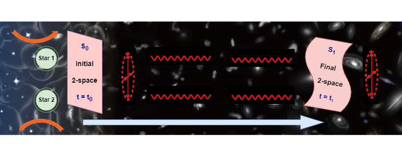
Figure 1: Schematic depiction of GW memory in LRS-II spacetime. The generated GWs (shown in red) are due to hyperbolic scattering between the two stars ($t=t_{0}$) which alter the shear of the 2-space at $t=t_{1}$. The blue arrow at the bottom depicts the direction of time ($u^{a}$). The orange arrows denote the trajectory of the stars.

A schematic depiction of the GW memory in the LRS-II spacetime is shown in Fig. 1. At $t=t_{0}$, the astrophysical process results in the generation of GWs. Assuming that the GWs travel from left to right, the generated GWs perturb the 2-D surface that is orthogonal to the direction of propagation in the semitetrad formalism. We are interested in the integrated effect of the GWs passing through the 2-D surface from $t=t_{0}$ to $t=t_{1}$. Before the generation of the GW ($t<t_{0}$), the LRS-II spacetime is described by the following geometrical variables [69]:

$$\mathcal{D}_{0}=\{\Theta,\phi,\Sigma,{\mathcal{A}},\mathcal{E}\}\cup\mbox{matter components},$$ (3)

where, $\Theta$ and $\phi$ represents expansion along $u^{a}$ and $n^{a}$, respectively, $\Sigma$ is component of shear tensor along $n^{a}$, $\mathcal{A}$ is the acceleration projected along $n^{a}$ of the comoving fictitious observer, and $\mathcal{E}$ is projection of electric-Weyl tensor along $n^{a}$. As mentioned above, all other geometrical variables vanish on the 2-D surface. This has to be contrasted with the covariant perturbation theory in cosmological spacetimes where the growth of tensor and scalar perturbations are generated due to the quantum fluctuations [76, 77].

GWs generated at $t=t_{0}$ permanently alter the 2-D surface, and the spacetime is no longer LRS-II. However, since the energy carried by the GWs is small, we can assume that the spacetime is a perturbed LRS-II. The perturbed spacetime will now contain non-zero geometrical variables on the 2-D surface. More specifically, it will contain non-zero components of the electric and magnetic Weyl $(\mathcal{E}_{a},\,\mathcal{E}_{ab},\,\mathcal{B}_{a},\,\mathcal{B}_{ab})$ and shear tensor $(\Sigma_{ab})$ that carries information about the incoming GW. Thus, the perturbed LRS-II spacetime is described by the following variables: $\mathcal{D}_{\rm n}\equiv\mathcal{D}_{0}\cup\{\mathcal{E}_{a},\,\mathcal{E}_{ab},\,\mathcal{B}_{a},\,\mathcal{B}_{ab},\,\Sigma_{ab}\}\cup\text{others}$, where $\{\mathcal{E}_{a},\,\mathcal{E}_{ab},\,\mathcal{B}_{a},\,\mathcal{B}_{ab},\,\Sigma_{ab}\}$ depend on the properties of the incoming GWs. For details, see the Appendix  A.

As mentioned above, the 2-D surface carries information about the passing GWs. Thus, to evaluate the GW memory of the perturbed LRS-II spacetime, we need to identify quantities related to the perturbed 2-D surface. In covariant formalism, the GW memory is related to the change in the geometrical quantities associated with the 2-D surface w.r.t the timelike direction $u^{a}$: $\mathcal{X}_{ab}=\mathcal{L}_{u}N_{ab}$. Since the GWs are symmetric and traceless, we have:

$$\mathcal{X}_{\{ab\}}=2\,\Sigma_{ab}\,.$$ (4)

For details, see Appendix (B). This identification is the key to obtaining the master equation for memory in LRS-II spacetime and we refer $\Sigma_{ab}$ as instantaneous memory tensor. This has to be contrasted with the cumulative memory $(\Delta N_{ab})$ which captures the integrated GW memory along the timelike vector. In this work, the final results are in terms of observables computed from the cumulative memory tensor.

III Master equation for memory in LRS-II spacetimes

In covariant formulation, like in 1+3 formulation, we write the perturbed Einstein’s equations in LRS-II spacetime into a set of evolution, propagation and constraint equations of electric $(\mathcal{E},\,\mathcal{E}_{a},\,\mathcal{E}_{ab})$ and magnetic parts $(\mathcal{B},\,\mathcal{B}_{a},\,\mathcal{B}_{ab})$ of Weyl tensor and the memory tensor ($\Sigma_{ab}$) [70]. To the first order in perturbations, the propagation equations (along the radial direction, denoted by over-hat, and the 2-space derivatives are given by $\delta$) for $\mathcal{E},\,\mathcal{B}$ are:

$$\hat{\mathcal{E}}=-\delta_{a}\mathcal{E}^{a}-3\phi\mathcal{E}/2;~{}~{}\hat{\mathcal{B}}=-\delta_{a}\mathcal{B}^{a}-3\phi\mathcal{B}/2\,.$$ (5)

Substituting these in the propagation equation and demanding that the electric and magnetic Weyl are orthogonal, we obtain the following constraints:

$$\mathcal{E}_{a}=\varepsilon_{ab}\mathcal{B}^{b}~{};~{}\mathcal{E}_{ab}=\varepsilon_{ad}\mathcal{B}^{d}\,_{b}$$ (6)

where, $\varepsilon_{ab}$ is Levi-Civita tensor in $2-$D surface. Substituting the above constraint leads to:

$$3\mathcal{E}\,\Sigma_{ab}+\left[2\Theta+3\Sigma+\phi\right]\mathcal{E}_{ab}+\left[\mu+p\right]\Sigma_{ab}=-\mathcal{G}_{ab}.$$ (7)

where, $\mathcal{G}_{ab}\equiv 2\,\epsilon_{c\{a}\delta^{c}\mathcal{B}_{b\}}$, captures the incoming GWs and the matter is represented by a perfect fluid with pressure $p$ and energy density $\mu$. The evolution of the instantaneous memory observable is,

$$\dot{\Sigma}_{\{ab\}}=-\left(\textstyle\frac{2}{3}\Theta+\textstyle\frac{1}{2}\Sigma\right)\Sigma_{ab}-\mathcal{E}_{ab}.$$ (8)

Substituting Eq. (8) in the constraint Eq (7) leads to the following master equation for GW memory:

$$\left(2\Theta+3\Sigma+\phi\right)\left[\dot{\Sigma}_{\{ab\}}+\left(\textstyle\frac{2}{3}\Theta+\textstyle\frac{1}{2}\Sigma\right)\Sigma_{ab}\right]$$

$$-\left[3\mathcal{E}\,+\mu+p\right]\Sigma_{ab}=\mathcal{G}_{ab}$$ (9)

Here, dot denotes derivative w.r.t timelike direction $u^{a}$. This is the key expression of this work, regarding which we want to discuss the following points: To begin with, the master equation relates the memory tensor and the geometrical quantities of the background spacetime along with the incoming GW. This equation is valid for all LRS-II spacetimes, including Minkowski, FLRW, and LTB cosmologies. However, all the earlier work on GW memory was restricted to asymptotically flat spacetime described by Bondi-Metzner-Sachs metric [78, 79, 80].

In addition, it is easy to verify that the above results match with Bondi shear for Minkowski spacetime [47]. $\phi(=2/r)$ is the only nonzero LRS scalar. Substituting $\phi$ in Eq. (III) and using the fact that $\dot{N}_{ab}=2\Sigma_{ab}$, we have:

$$2\,\dot{\Sigma}_{ab}=r\,\mathcal{G}_{ab}~{}~{}\Longrightarrow~{}~{}\ddot{N}_{ab}=r\,\mathcal{G}_{ab}\,.$$ (10)

where dot denotes partial derivative w.r.t. the retarted time coordinate $u$. Since the GW memory depends on the incoming GW, to keep calculations transparent, we assume the incoming GW to have a burst profile ($h_{ab}^{I}$) due to hyperbolic scattering between two stars [81]. Simulations of PBHs in galaxy clusters reveal numerous hyperbolic encounters where two BHs interact, emitting GW Bremsstrahlung [82]. For close enough encounters, the GWs emitted may be detectable in the present and future GW detectors [83, 84]. Evaluating the electric and magnetic parts of the Weyl tensor for the plus polarization of the incoming GW, we get [85]:

$$\ddot{N}_{\vartheta\vartheta}(u)=r^{2}\,\cos\vartheta\,\cos(2\varphi)\,\ddot{h}_{\vartheta\vartheta}^{I}(u)\,.$$ (11)

Details of the burst profile are irrelevant to the present discussion. (See Appendix D.) Integrating the above equation for a finite time $(t_{0},t_{1})$ interval, we get $\Delta N_{\vartheta\vartheta}\sim r^{2}\Delta h_{\vartheta\vartheta}^{I}$. Since the GW burst falls as $\mathcal{O}(1/r)$, we find the memory observable in our formalism scale as $\mathcal{O}(r)$. Thus, it is a subleading term, much akin to the Bondi shear [47]. See also Appendix D. Thus, our analysis reveals the conventional non-oscillatory behavior of the memory observable such that the final spacetime is a shifted Minkowski [40, 47] (See Fig. 3). Furthermore, Eq.(11) resembles a forced system, where the incoming GW provides the forcing term. Such forced systems have been discussed earlier in literature in Ref. [39, 58].

Lastly, the master equation (III) is a crucial step towards future observational implications of GW memory as it explicitly contains the non-linear dependence of the background quantities. For instance, the earlier work on GW memory in cosmological settings did not account for the non-linear dependence  [56]. Like in the electromagnetic memory [65], this analysis shows that the GW memory contains a non-linear contribution of the geometry, which is a quintessential property of gravity! We now show that cosmological GW memory provides a distinct signature in identifying cosmological transition redshift.

IV Cosmological GW memory

Consider the following spatially flat FLRW line-element $ds^{2}=a^{2}(\eta)[-d\eta^{2}+d{\bf x}^{2}]$, where $\eta$ is conformal time, $a(\eta)$ is the scale factor and $d{\bf x}^{2}$ is 3-space. In FLRW spacetime, $\Theta=3{\mathcal{H}}/a,{\mathcal{H}}={a^{\prime}}{/a}\equiv d(\ln a)/d\eta$ and $\Sigma=-\Theta/3$ are non-zero [86]. Substituting these in Eq. (III) reduces to:

$$2\,\Theta\,\dot{\Sigma}_{ab}+\Theta^{2}\,\Sigma_{ab}-2\,(\mu+p)\,\Sigma_{ab}=2\,\mathcal{G}_{ab}\,,$$ (12)

where dot refers to the retarded time $\tilde{u}=\eta-r$ and $\mu,p$ refer to the energy density and pressure of the cosmological fluid. This is the second key expression of this work regarding which we want to discuss the following points. First, unlike Minkowski, $\phi$ contributes to the subleading terms. Due to homogeneity and isotropic nature of the FLRW, $\Theta,\mu$, and $p$ do not have any radial dependence. Hence, asymptotic (large $r$) behavior of the GW memory in FLRW is different from Minkowski as the LRS scalars governing their evolution have different fall-offs. Thus, in FLRW, $\Sigma_{ab}$ does not have $\mathcal{O}(1/r)$ fall-off. This feature is unique from our analysis.

Second, this can be understood from the Lagrangian and Eulerian viewpoint in fluid mechanics. The asymptotic static observers in Minkowski spacetime correspond to Eulerian observers, while, the comoving observers in FLRW spacetime are Lagrangian. Hence, unlike in Minkowski spacetime, we do not have to transform the above expression to Eulerian observers [65]. This was missed in the earlier works on memory in cosmological settings. Since cosmological memory of the comoving observers do not have $\mathcal{O}(1/r)$ fall-off, this provides unique opportunity to have observable consequences.

To understand the consequence, we consider an incoming (plus polarization) GW burst produced due to hyperbolic scattering between two stars at time $\eta_{0}$, and after traversing through the Universe reaches us at $\eta=\eta_{1}$. Since we are interested in the time evolution of the amplification factor, keeping $r$ fixed, rewriting $\tilde{u}$ in-terms of $\eta$, Eq. (12) reduces to:

$$\Sigma_{\vartheta\vartheta}^{\prime}\,+\Gamma(\eta)\,\Sigma_{\vartheta\vartheta}=({a(\eta)}/{3{\mathcal{H}}})\,r\cos\vartheta\cos(2\varphi)\,h_{\vartheta\vartheta}^{I^{\prime\prime}}(\eta)$$ (13)

where, $\Gamma(\eta)=-c_{0}{\mathcal{H}}+c_{1}{{\mathcal{H}}^{\prime}}/{{\mathcal{H}}}$,   $c_{0}={1}/{2}+c_{1}$, and $c_{1}={1}/{(12\pi)}$. In terms of $N_{\vartheta\vartheta}$, Eq. (13) reads as:

$$\left[\frac{N_{\vartheta\vartheta}}{a^{2}}\right]^{\prime\prime}\!\!+({\mathcal{H}}+\Gamma)\left[\frac{N_{\vartheta\vartheta}}{a^{2}}\right]^{\prime}\!\!=\frac{2r}{3{\mathcal{H}}}\cos\vartheta\cos(2\varphi)\,h_{\vartheta\vartheta}^{I^{\prime\prime}}$$ (14)

As mentioned above, $N_{\vartheta\vartheta}\sim\mathcal{O}(1)$ fall-off at asymptopia. Hence, unlike in Minkowski (11), the damping term play a crucial role in the cosmological memory. Specifically, the form of ${\cal H}$ and ${\cal H}^{\prime}$ determine the cumulative memory at the final time $\eta_{1}$. Physically, the successive waves generated have a smaller magnitude than their predecessors, however, integrated over cosmological time lead to observable signatures.

Since GWs are massless, the energy density scales as $N_{\vartheta\vartheta}^{2}/a^{4}$. To understand the effect of background geometry on GW memory, we compute the amplification factor ($A_{C}$) which is the ratio of GW memory amplitude at the final and initial time. For the previously discussed GW burst, we have:

$$\!\!\!\!A_{C}=\frac{\left({N_{\vartheta\vartheta}}/{a^{2}}\right)\rvert_{\eta_{1}}}{\left({N_{\vartheta\vartheta}}/{a^{2}}\right)\rvert_{\eta_{0}}}=1+\dfrac{a^{2}(\eta_{0})}{h_{I}(\eta_{0})}\,[F(\eta_{1})-F(\eta_{0})].$$ (15)

For details, see Appendix D.2. We are now in a position to understand the relation between the amplification factor and cosmological epochs. To go about this, we consider three scenarios — matter dominated (MD), dark energy (DE) dominated and matter to $\Lambda$ dominated [11].

Fig.(2) is the plot of $A_{C}$ as a function of cosmic time ($t$). For MD and DE, we have assumed one e-folding of expansion and the final times are chosen to be identical. In the case of matter to $\Lambda$ dominated, we have used Sahni and Starobinsky exact solution $a(t)=\sinh^{2/3}(\textstyle\frac{3}{2}t)$ [11] which transitions between a MD universe to deSitter (dS) at $t\to 0$ and $t\to+\infty$, respectively. In this case, we have considered a larger range to show the imprint of transition in the amplification factor. All the scenarios show a gradual change in $A_{C}$. While $A_{C}$ decays for both DE and MD, it increases at the transition epoch for the matter to $\Lambda$ dominated scenario. As a result, we can use $A_{C}$, the cosmological memory-related amplification factor, to detect the cosmological transition redshift.

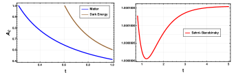
Figure 2: The evolution of the amplification factor ($A_{C})$ for three scenarios as a function of cosmic time. Left plot: Matter $a(t)=t^{2/3}$ and Dark energy, $a(t)=t^{2}$. Right Plot: Sahni-Starobinsky model, $a(t)=\sinh^{2/3}(\textstyle\frac{3}{2}t)$ [11].

V Conclusions and Observational Implications

GW memory, yet to be detected from observations, provides an interesting avenue for understanding features of strong-field gravity. However, prior to this work, there did not exist a unified formalism for studying GW memory for a larger class of spacetimes. Our work tries to fill this gap by constructing a master equation for a class of background geometries known as LRS-II spacetimes. We showed that the Master equation for Minkowski spacetime leads to Bondi shear. In the case of FLRW spacetime, we showed that the cosmological memory does not have a $\mathcal{O}(1/r)$ fall-off, thus providing a unique opportunity to be used as an observational probe. Additionally, the cumulative cosmological memory bears similarity to the formation of large-scale structures in the universe through the growth of density perturbations.

Our analysis shows that the cosmological memory has the potential to identify the epoch of matter to $\Lambda$ transition. This work gives a novel proof-of-principle to capture cosmological transition redshift ($z_{t}$) by the measurement of GW memory. Till date, most prescriptions have either relied upon the cosmic ladder (SNe) [87, 88] or the cosmic distance approaches (BAO) [89]. Independent estimates by using expansion rate of passively evolving galaxies [25] along with Planck missions [90] have constrained the value at $z_{t}=0.64^{+0.11}_{-0.07}$ for $\Lambda$CDM model. Viable cosmological models in $f(R)$ and $f(T)$ gravity theories have set $z_{t}$ as $0.7679^{+0.1831}_{-0.1829}$ and $0.643^{0.034}_{-0.030}$ [91, 92]. Thus, there exists parameter range where $z_{t}$ can be further constrained.

We outline two avenues where our work can provide crucial pointers in cosmology and GW science. First, our methodology only employs the measurement of GW memory. The obtained memory signal would provide a signature of the source redshift and the corresponding era of the universe. Second, knowing the source distance from the oscillatory part of the GW signal along with redshift of the host galaxy from EM data, one can compare our results and provide better constraints to both cosmological models as well as theory of gravity. These are currently under investigation.

Acknowledgement: The authors thank R. Goswami, J. P. Johnson, S. Kar, A. Kushwaha, and S. Mandal for discussions and comments on the earlier draft. The work is supported by SERB-CRG (RD/0122-SERB000-044). Thanks to Einstein Telescope team for providing the background for Fig. 1.

Appendix A Semitetrad covariant formalism

In this section, we briefly recapitulate the semi-tetrad formalism [93, 69], which enables us to study GW memory for LRS-II spacetime. A crucial feature of these semi-tetrad decompositions is their locality, defined on any open set $\mathcal{S}$. Initially, the properties of spacetime are analyzed relative to a real or fictitious observer whose velocity aligns with the tangent of a timelike congruence, splitting the $4-$d spacetime into a timelike direction and a $3-$space. Subsequently, if the spacetime exhibits certain symmetries such as local rotational symmetry, a preferred spatial direction emerges. The spacetime is further decomposed using this preferred spatial congruence. The field equations are then reformulated in terms of the geometric variables associated with these congruences and the curvature tensor of the spacetime (appropriately decomposed using the congruences).

Although this formalism is well-studied in the literature [70], for completeness, we provide a overview of the same.

A.1 Semitetrad 1+3 formalism

Covariant formalism, first proposed in Refs. [94, 95], later were extensively used in relativistic comlogy [77]. In this formalism the $4-$d spacetime is deconstructed w.r.t a fictitious co-moving observer, moving with velocity $u^{a}=dx^{a}/d\tau$($\tau$ is the affine parameter), satisfying $u_{a}u^{a}=-1$. The spacetime comprises a timelike congruence $\gamma$ and a $3-$d space orthogonal to $u^{a}$. The $3-$d space is described by the projection tensor $h_{ab}$ that follows:

$$g_{ab}=-u_{a}\hskip 0.99594ptu_{b}+h_{ab},$$ (16)

iff the 3-space has no twist or vorticity, $h_{ab}$ becomes metric of the $3-$space. The covariant time derivative along the observers’ worldlines, denoted by ‘${\hskip 0.99594pt\hskip 0.99594pt{}^{\cdot}\hskip 0.99594pt\hskip 0.99594pt}$’, is defined using the vector ${u^{a}}$, as

$$\dot{Z}^{a...b}{}_{c...d}=u^{e}\hskip 0.99594pt\nabla_{e}\hskip 0.99594ptZ^{a...b}{}_{c...d},$$ (17)

for any tensor ${Z^{a...b}{}_{c...d}}$. The fully orthogonally projected covariant spatial derivative, denoted by ‘ ${D}$ ’, is defined using the spatial projection tensor ${h_{ab}}$, as

$$D_{e}\hskip 0.99594ptZ^{a...b}{}_{c...d}=h^{r}{}_{e}h^{a}{}_{f}\hskip 0.99594pt...\hskip 0.99594pth^{b}{}_{g}\hskip 0.99594pth^{p}{}_{c}\hskip 0.99594pt...\hskip 0.99594pth^{q}{}_{d}\hskip 0.99594pt\nabla_{r}\hskip 0.99594ptZ^{f...g}{}_{p...q},$$ (18)

The covariant derivative of the 4-velocity vector ${u^{a}}$ is decomposed irreducibly as follows

$$\nabla_{a}\hskip 0.99594ptu_{b} = -u_{a}\hskip 0.99594ptA_{b}+\frac{1}{3}h_{ab}\hskip 0.99594pt\Theta+\sigma_{ab}+\epsilon_{abc}\hskip 0.99594pt\omega^{c},$$ (19)

where ${A_{b}}$ is the acceleration, ${\Theta}$ is the expansion of ${u_{a}}$, ${\sigma_{ab}}$ is the shear tensor, ${\omega^{a}}$ is the vorticity vector representing rotation and ${\epsilon_{abc}}$ is the effective volume element in the rest space of the comoving observer. The vorticity vector $\omega^{q}$ is related to vorticity tensor $\omega^{ab}$ as: $\omega^{a}\equiv(1/2)\,\epsilon^{abc}\,\omega_{bc}$.

Furthermore, the energy-momentum tensor of matter or fields present in the spacetime, decomposed relative to ${u^{a}}$, is given by

$$T_{ab} = \mu\hskip 0.99594ptu_{a}\hskip 0.99594ptu_{b}+p\hskip 0.99594pth_{ab}+q_{a}\hskip 0.99594ptu_{b}+u_{a}\hskip 0.99594ptq_{b}+\pi_{ab},$$ (20)

where ${\mu}$ is the effective energy density, ${p}$ is the isotropic pressure, ${q_{a}}$ is the 3-vector defining the energy-momentum flux and ${\pi_{ab}}$ is the anisotropic stress. The Weyl tensor also is decomposed into electric part $E_{ab}$ and magnetic part $B_{ab}$ as follows,

$$E_{ab} = C_{acbd}\hskip 0.99594ptu^{c}\hskip 0.99594ptu^{d}=E_{<ab>},$$ (21)

$$B_{ab} = \frac{1}{2}\varepsilon_{ade}\hskip 0.99594ptC^{de}{}_{bc}\hskip 0.99594ptu^{c}=B_{<ab>}.$$ (22)

Here, the angle brackets denote orthogonal projections of vectors onto the three space as well as the projected, symmetric and trace-free (PSTF) part of tensors:

$$\dot{V}_{<a>} = h_{a}{}^{b}\hskip 0.99594pt\dot{V}_{b},$$ (23)

$$Z_{<ab>} = \left(h^{c}{}_{(a}\hskip 0.99594pth^{d}{}_{b)}-\frac{1}{3}h_{ab}\hskip 0.99594pth^{cd}\right)\hskip 0.99594ptZ_{cd}.$$ (24)

A.2 Semitetrad 1+1+2 formalism

The $3-$space mentione din the $1+3$ covariant formalism can be further split into a one spaclike direction $e_{a}$ satisfying $e_{a}e^{a}=1$ and a $2-$d surface orthogonal to both $u^{a}$ and $e^{a}$. The 1+1+2 covariantly decomposed spacetime is expressed in terms of the projection tensor $N_{ab}$ associated to the $2-$d surface as:

$$g_{ab}=-u_{a}\hskip 0.99594ptu_{b}+e_{a}\hskip 0.99594pte_{b}+N_{ab},$$ (25)

where ${N_{ab}}$ ${\left(e^{a}\hskip 0.99594ptN_{ab}=0=u^{a}\hskip 0.99594ptN_{ab},N^{a}{}_{a}=2\right)}$ projects vectors onto the 2-sheets, orthogonal to ${u^{a}}$ and ${e^{a}}$. We introduce two new derivatives for any tensor ${\phi_{a...b}{}^{c...d}}$:

$$\hat{\phi}_{a..b}{}^{c..d} \equiv e^{f}\hskip 0.99594ptD_{f}\hskip 0.99594pt\phi_{a..b}{}^{c..d},$$ (26)

$$\delta_{f}\phi_{a...b}{}^{c...d} \equiv N_{f}{}^{j}N_{a}{}^{l}...N_{b}{}^{g}N_{h}{}^{c}...N_{i}{}^{d}D_{j}\phi_{l...g}{}^{h...i}.$$

Eq.(26) denotes the derivative along the preferred spacelike direction $e^{a}$ while $\delta_{f}$ in Eq.(A.2) gives the 2-space derivative.

The 1+3 geometrical and dynamical quantities and anisotropic fluid variables are split irreducibly as

$$A^{a} = \mathcal{A}\hskip 0.99594pte^{a}+\mathcal{A}^{a},$$ (28)

$$\omega^{a} = \Omega\hskip 0.99594pte^{a}+\Omega^{a},$$ (29)

$$\sigma_{ab} = \Sigma\left(e_{a}\hskip 0.99594pte_{b}-\frac{1}{2}\hskip 0.99594ptN_{ab}\right)+2\hskip 0.99594pt\Sigma_{(a}\hskip 0.99594pte_{b)}+\Sigma_{ab},$$ (30)

$$E_{ab} = \mathcal{E}\left(e_{a}\hskip 0.99594pte_{b}-\frac{1}{2}\hskip 0.99594ptN_{ab}\right)+2\hskip 0.99594pt\mathcal{E}_{(a}\hskip 0.99594pte_{b)}+\mathcal{E}_{ab},$$ (31)

$$B_{ab} = \mathcal{H}\left(e_{a}\hskip 0.99594pte_{b}-\frac{1}{2}\hskip 0.99594ptN_{ab}\right)+2\hskip 0.99594pt\mathcal{H}_{(a}\hskip 0.99594pte_{b)}+\mathcal{H}_{ab}\,.$$ (32)

The fully projected 3-derivative of ${e^{a}}$ is given by

$$D_{a}\hskip 0.99594pte_{b} = e_{a}\hskip 0.99594pta_{b}+\frac{1}{2}\hskip 0.99594pt\phi\hskip 0.99594ptN_{ab}+\xi\hskip 0.99594pt\varepsilon_{ab}+\zeta_{ab},$$ (33)

where traveling along ${e^{a}}$, ${a_{a}}$ is the sheet acceleration, ${\phi}$ is the sheet expansion, ${\xi}$ is the vorticity of ${e^{a}}$ (the twisting of the sheet) and ${\zeta_{ab}}$ is the shear of ${e^{a}}$.

We can immediately see that the Ricci identities and the doubly contracted Bianchi identities, which specify the evolution of the complete system, can now be written as the time evolution, spatial propagation, and spatial constraints of an irreducible set of geometrical variables:

$$\mathcal{D}_{geom}= \{\Theta,\hskip 0.99594pt\mathcal{A},\hskip 0.99594pt\Omega,\hskip 0.99594pt\Sigma,\hskip 0.99594pt\mathcal{E},\hskip 0.99594pt\mathcal{B},\hskip 0.99594pt\phi,\hskip 0.99594pt\xi,\hskip 0.99594pt\mathcal{A}_{a},\hskip 0.99594pt\Omega_{a},\hskip 0.99594pt\Sigma_{a},\hskip 0.99594pt\alpha_{a},\hskip 0.99594pta_{a},\hskip 0.99594pt\mathcal{E}_{a},$$

$$\hskip 0.99594pt\mathcal{B}_{a},\hskip 0.99594pt\Sigma_{ab},\hskip 0.99594pt\zeta_{ab},\hskip 0.99594pt\mathcal{E}_{ab},\hskip 0.99594pt\mathcal{B}_{ab}\}$$ (34)

A.3 Degrees of freedom of incoming GW

Let us consider the following scenario: As show in Fig. (3), LRS-II spacetime is perturbed due to the incoming GW. This disturbs the LRS-II spacetime and leads to GW memory. To identify the GW memory, we need to know the true GW degrees of freedom (DOF) in this formalism. In this appendix, for completeness, we identify the true GW DOF.

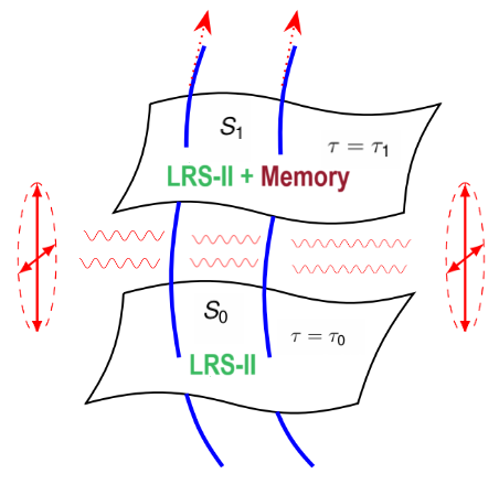
Figure 3: The presence of GW alters the background LRS spactime.

Let the initial LRS-II spacetime be represented by the geometric variables $\mathcal{D}_{0}$. Due to the incoming GW, the spacetime is no more LRS-II. Since the incoming GW is weak, we can assume that the resulting spacetime to be perturbed LRS-II. Let us represent the geometric variables of this spacetime as $\mathcal{D}_{\rm n}$.

The GW mimicking variable may consist of one or several vector or tensor quantities listed in $\mathcal{D}_{\rm n}$. As described in Refs. [72, 73], the Weyl curvature tensor $C_{abcd}$ characterizes the gravitational distortion or perturbation caused by GWs. The electric part of the Weyl tensor, denoted by the 3-tensor $E_{ab}$, provides information about the tidal deformation in spacetime, while the magnetic part, represented by $H_{ab}$, presents the gravitational radiation traveling to future infinity from the source [72, 71]. Both the electric and magnetic parts of the Weyl tensor follow a closed form of the wave equation in the FLRW spacetime [96, 71].

In the $1+3$ formalism, $H_{ab}$ and $E_{ab}$ represent certain features of GWs, while in the $1+1+2$ formalism, their components such as $\mathcal{B},,\mathcal{B}_{a},,\mathcal{B}_{ab}$ and $\mathcal{E},,\mathcal{E}_{a},,\mathcal{E}_{ab}$ carry information about the passing GWs during $[\tau_{0},,\tau_{1}]$. As mentioned earlier, GWs perturb the $2-$dimensional surface $S_{0}$ orthogonal to it. Hence, the vector and tensor components of $H_{ab}$ and $E_{ab}$ in the $2-$dimensional surface ($\mathcal{B}_{a},,\mathcal{B}_{ab}$) and ($\mathcal{E}_{a},,\mathcal{E}_{ab}$) describe the GW distortion during the time interval $[\tau_{0},,\tau_{1}]$.

As discussed above, in the $1+1+2$ formalism $\mathcal{E}_{a},,\mathcal{E}_{ab},,\mathcal{B}_{a},,\mathcal{B}_{ab}$ each have two components, resulting in a total of 8 DOF. However, considering the 2 constraint equations for the scalar part of electric and magnetic Weyl (45),(46), the DOF reduces to 6. Furthermore, the relationship among the components of the electric and magnetic parts of the Weyl tensor, as given by Eq.(53), (54) in the Appendix (C), reduces the DOF to 2, matching the DOF of GWs in linearized gravity theory [97, 73]. In principle, any of $\mathcal{E}_{a},,\mathcal{E}_{ab},,\mathcal{B}_{a},,\mathcal{B}_{ab}$ can represent the passing gravitational wave. However, to formulate the master equation for GW memory as done in Appendix (C), we choose $\mathcal{B}_{a}$ to describe the incoming GW.

Appendix B Relation between GW memory and shear

Gravitational wave (GW) memory refers to the change in the metric or spacetime resulting from the passage of GWs. Mathematically, it is defined as:

$$\Delta h_{+,\times}^{\mathrm{mem}}=\lim_{t\rightarrow+\infty}h_{+,\times}(t)-\lim_{t\rightarrow-\infty}h_{+,\times}(t),$$ (35)

where $t$ represents the time of the asymptotic (static) observer, and $h_{+}$ and $h_{\times}$ denote the plus and cross modes of the GW signal, respectively.

However, in covariant formalism, $u^{a}$ defines the time. The change of any vector or tensor with respect to time is equivalent to their covariant derivative projected along the timelike direction $u^{a}$. This change can be obtained from the Lie derivative of any tensor or vector along $u^{a}$. To quantify gravitational memory and relate it to the geometrical variables described in $\mathcal{D}_{\rm n}$, we begin with the Lie derivative of $N_{ab}$ along $u^{a}$.

$$\mathcal{X}_{ab}\equiv\mathcal{L}_{u}N_{ab}=u^{c}\nabla_{c}N_{ab}+N_{cb}\nabla_{a}u^{c}+N_{ca}\nabla_{b}u^{c}$$ (36)

Substituting the geometrical variables described in $1+1+2$ formalism we obtain,

$$\mathcal{X}_{ab}=2n_{(a}\left[-\alpha_{b)}+\Sigma_{b)}-\varepsilon_{b)\,c}\,\Omega^{c}\right]+2\,\Sigma_{ab}$$

$$+N_{ab}\left[\frac{2\Theta}{3}-\Sigma\right]$$ (37)

The brackets $()$ in the subscript denote the symmetrization of the terms. In Ref. [70], the author mentions the existence of a $2-$surface if the Greenberg vector $\Sigma^{a}+\varepsilon^{ab}\Omega_{b}-\alpha^{a}=0$. Using this Greenberg vector condition in the previous equation, we obtain:

$$\mathcal{X}_{ab}=-4n_{(a}\varepsilon_{b)c}\,\Omega^{c}+2\Sigma_{ab}+N_{ab}\left(\frac{2\Theta}{3}-\Sigma\right)$$ (38)

The quantity $\mathcal{X}_{ab}$ above is symmetric but not transverse-traceless. Its transverse trace-less part is derived as follows:

$$\mathcal{X}_{\{ab\}}=N^{\alpha}\,_{(a}N^{\beta}\,_{b)}\mathcal{X}_{cd}-\frac{1}{2}N_{ab}N^{cd}\mathcal{X}_{cd}$$ (39)

Substituting $\mathcal{X}_{\alpha\beta}$ into the RHS of the above equation, we finally obtain:

$$\mathcal{X}_{\{ab\}}=2\,\Sigma_{ab}$$ (40)

The $\Sigma_{ab}$ tensor serves as an indicator of memory in this scenario as it represents the time evolution of the projection tensor onto the $2-$space. We need to establish the conditions under which the projection tensor $N_{ab}$ reduces to the metric of the $2-$space. These conditions are: 1) the Greenberg vector $\Sigma^{a}+\varepsilon^{ab}\Omega_{b}-\alpha^{a}=0$, and 2) $\xi=\Omega=0$).

Similarly, the covariant derivative of $N_{ab}$ projected along the spacelike direction will be $\zeta_{ab}$, where $\zeta_{ab}$ represents the shear related to the spacelike direction $n^{a}$. Hence, both $\sigma_{ab}$ and $\zeta_{ab}$ will contribute to memory.

In the following calculation, we assume that the projection tensor $N_{ab}$ reduces to the metric of the $2-$space if:

$$\text{Greenberg vector:}\quad\Sigma^{a}+\varepsilon^{ab}\Omega_{b}-\alpha^{a} =0,$$ (41)

$$\text{}\xi=\Omega =0$$ (42)

are satisfied.

Appendix C Formulation of gravitational memory in LRS-II spacetime

In this section we formulate the master equation to obtain GW memory in the LRS-II spacetime using the evolution, propagation and constraint equations of electric $\mathcal{E},\,\mathcal{E}_{a},\,\mathcal{E}_{ab}$ and magnetic parts $\mathcal{B},\,\mathcal{B}_{a},\,\mathcal{B}_{ab}$ of Weyl curvature tensor. Here, we use the equations derived in Ref. [70] considering terms till first order w.r.t. the quantities listed in $\mathcal{D}_{\rm n}$. We assume that the LRS-II background contains only the energy density and pressure in the energy-momentum tensor that is a function of time along. We ignore the anisotropic stress and heat flux. The propagation equations for $\mathcal{E},\,\mathcal{B}$ are:

$$\hat{\mathcal{E}} =-\delta_{a}\mathcal{E}^{a}-\frac{3}{2}\phi\mathcal{E}$$ (43)

$$\hat{\mathcal{B}} =-\delta_{a}\mathcal{B}^{a}-\frac{3}{2}\phi\mathcal{B}$$ (44)

As GWs propagate along the null direction, instead of using the time coordinate $t$’ and radial coordinate $r$’, we utilize the null coordinate $u\equiv t-r$. In an asymptotically flat spacetime, at the asymptotic limit, the time and radial derivatives can be expressed as $\partial_{t}\sim\partial_{u}$ and $\partial_{r}\sim-\partial_{u}$. Using this notation, we rewrite the propagation equations as follows:

$$\partial_{u}\mathcal{E}-\frac{3}{2}\phi,\mathcal{E} =\delta_{a}\mathcal{E}^{a}$$ (45)

$$\partial_{u}\mathcal{B}-\frac{3}{2}\phi,\mathcal{B} =\delta_{a}\mathcal{B}^{a}$$ (46)

These are the constraint equations relating the scalar part $\mathcal{E}(\mathcal{B})$ to the vector $\mathcal{E}_{a}(\mathcal{B}_{a})$. Now, we aim to establish if there exists any relation between the electric and magnetic parts of the Weyl tensor. To proceed, we derive the evolution equations for $\mathcal{E}_{a}$ and $\mathcal{B}_{a}$ after incorporating conditions (41) and (42) in the null coordinate.

$$\partial_{u}\mathcal{E}_{a}-\frac{1}{2}\varepsilon_{ab}\partial_{u}\mathcal{B}^{b} =\frac{3}{4}\varepsilon_{ab}\delta^{b}\mathcal{B}+\frac{1}{2}\varepsilon_{bc}\delta^{b}\mathcal{B}^{c}\,_{a}-\frac{1}{2}(\mu+p)\,\Sigma_{a}$$

$$+\left(\frac{3}{4}\Sigma-\Theta\right)\mathcal{E}_{a}-\left(\frac{1}{4}\phi+\mathcal{A}\right)\varepsilon_{ab}\mathcal{B}^{b}$$ (47)

and,

$$\partial_{u}\mathcal{B}_{a}+\frac{1}{2}\varepsilon_{ab}\partial_{u}\mathcal{E}^{b} =-\frac{3}{4}\varepsilon_{ab}\delta^{b}\mathcal{E}-\frac{1}{2}\varepsilon_{bc}\delta^{b}\mathcal{E}^{c}\,_{a}$$

$$+\left(\frac{3}{4}\Sigma-\Theta\right)\mathcal{B}_{a}+\left(\frac{1}{4}\phi+\mathcal{A}\right)\varepsilon_{ab}\mathcal{E}^{b}$$ (48)

We write the propagation equations of $\mathcal{E}_{a},\,\mathcal{B}_{a}$ in terms of null coordinate as follows,

$$\partial_{u}\mathcal{E}_{a} =-\frac{1}{2}\delta_{a}\mathcal{E}+\delta^{b}\mathcal{E}_{ab}+\frac{3}{2}\phi\mathcal{E}_{a}+\frac{3}{2}\Sigma\,\varepsilon_{ab}\mathcal{B}^{b}$$ (49)

and,

$$\partial_{u}\mathcal{B}_{a} =-\frac{1}{2}\delta_{a}\mathcal{B}+\delta^{b}\mathcal{B}_{ab}+\frac{3}{2}\phi\mathcal{B}_{a}-\frac{3}{2}\Sigma\varepsilon_{ab}\mathcal{E}^{b}$$ (50)

Now, multiplying Eq. (C) with $\varepsilon^{ae}$ and adding it to Eq. (C) (by setting the same dummy index to $a$) we obtain the following relation,

$$\frac{3}{2}\partial_{u}\left(\mathcal{E}_{a-}\varepsilon_{ab}\mathcal{B}^{b}\right)=\frac{3}{4}\left(\varepsilon_{ab}\delta^{b}\mathcal{B}-\delta_{a}\mathcal{E}\right)-\frac{1}{2}\left(\mu+p\right)\Sigma_{a}$$

$$-\frac{3}{4}\left(\alpha_{a}-2\mathcal{A}_{a}\right)\mathcal{E}+\left(\frac{\phi}{4}+\mathcal{A}+\frac{3}{4}\Sigma-\Theta\right)\left(\mathcal{E}_{a}-\varepsilon_{ab}\mathcal{B}^{b}\right)$$

$$+\frac{1}{2}\left(\varepsilon_{bc}\delta^{b}\mathcal{B}^{c}\,_{a}-\delta^{b}\mathcal{E}_{ab}\right)$$ (51)

Substituting Eqs. (49) and (50) into the above equation and multiplying the result by $\varepsilon^{ad}$ we obtain,

$$2\delta^{b}\left(\mathcal{E}_{ab}-\varepsilon^{ad}\mathcal{B}^{d}\,_{b}\right) +2(\mu+p)\Sigma_{a}=$$

$$\left(-2\phi+\mathcal{A}+3\Sigma-\Theta\right)\left(\mathcal{E}_{a}-\varepsilon_{ab}\mathcal{B}^{b}\right)$$ (52)

One can check that $\alpha_{a}$=0 for perturbed FLRW and Minkowski spacetimes. This automatically ensures that $\Sigma_{a}=0$ if $\Omega_{a}=0$ from the Greenberg vector condition. We choose in rest of our work the following relation between $\{\mathcal{E}_{a},\,\mathcal{B}_{a}\}$ and $\{\mathcal{E}_{ab},\,\mathcal{B}_{ab}\}$.

$$\mathcal{E}_{a}=\varepsilon_{ab}\mathcal{B}^{b}$$ (53)

$$\mathcal{E}_{ab}=\varepsilon_{ad}\mathcal{B}^{d}\,_{b}$$ (54)

We have the evolution equation of $\mathcal{E}_{ab}$, tensor part of the electric part of Weyl tensor in null coordinate as,

$$\partial_{u}\mathcal{E}_{\{ab\}}+\partial_{u}\left(\varepsilon_{c\{a}\mathcal{B}_{b\}}^{~{}~{}c}\right)=-\varepsilon_{c\{a}\delta^{c}\mathcal{B}_{b\}}-\textstyle\frac{3}{2}\mathcal{E}\Sigma_{ab}$$

$$-\textstyle\frac{3}{2}\mathcal{B}\varepsilon_{c\{a}\zeta_{b\}}^{~{}~{}c}-\left(\Theta+\textstyle\frac{3}{2}\Sigma\right)\mathcal{E}_{ab}+\left(\textstyle\frac{1}{2}\phi+2{\cal A}\right)\varepsilon_{c\{a}\mathcal{B}_{b\}}^{~{}~{}c}$$

$$-\textstyle\frac{1}{2}(\mu+p)\Sigma_{ab}$$ (55)

We have assumed $\partial_{u}\varepsilon_{ab}=0$. Now substituting Eq. (54) relation and simplifying the above equation we obtain,

$$3\mathcal{E}\,\Sigma_{ab}+\left(2\Theta+3\Sigma+\phi+4\mathcal{A}\right)\mathcal{E}_{ab}+\left(\mu+p\right)\Sigma_{ab}$$

$$=-2\varepsilon_{c\{a}\delta^{c}\,\mathcal{B}_{b\}}$$ (56)

We already mentioned that the shear tensor $\Sigma_{ab}$ holds information about the alteration of the spacetime or the memory the passing GW. Hence we want to re-write the above Eq. (C) substituting $\mathcal{E}_{ab}$ in terms of $\Sigma_{ab}$. To do so, we have the evolution equation of $\Sigma_{ab}$ as,

$$\dot{\Sigma}_{\{ab\}}=\delta_{\{a}{\cal A}_{b\}}-\left(\textstyle\frac{2}{3}\Theta+\textstyle\frac{1}{2}\Sigma\right)\Sigma_{ab}+\mathcal{A}\zeta_{ab}-\mathcal{E}_{ab}$$ (57)

We set $\mathcal{A}=\mathcal{A}_{a}=0$ in the above equation and obtain,

$$\mathcal{E}_{ab}=-\dot{\Sigma}_{\{ab\}}-\left(\textstyle\frac{2}{3}\Theta+\textstyle\frac{1}{2}\Sigma\right)\Sigma_{ab}$$ (58)

Substituting Eq. (58) into Eq. (C) we obtain the final master equation for GW memory,

$$3\mathcal{E}\,\Sigma_{ab}-\left(2\Theta+3\Sigma+\phi\right)\dot{\Sigma}_{\{ab\}}+\left(\mu+p\right)\Sigma_{ab}$$

$$-\left(2\Theta+3\Sigma+\phi\right)\left(\textstyle\frac{2}{3}\Theta+\textstyle\frac{1}{2}\Sigma\right)\Sigma_{ab}=-2\varepsilon_{c\{a}\delta^{c}\,\mathcal{B}_{b\}}$$ (59)

Appendix D Gravitational wave memory profiles in Minkowski and FLRW spacetime

In this section, we try to examine the behavior of the memory observable ($N_{\vartheta\vartheta}$) in Minkowski spacetime and the amplification factor ($A_{C}$) in FLRW.

D.1 Minkowski spacetime

As previously outlined, the fall-off behavior of the memory observable in Minkowski spacetime is $1/r$. Assuming the form of the incoming GW profile for the plus polarization to be [81]:

$$h_{+}^{I}= 4,{\dfrac{m_{A}m_{B}}{b,r}},\bigg{[}\frac{1}{4}\left(\frac{1}{\sqrt{l^{2}+1}}+\frac{1}{\left(l^{2}+1\right)^{3/2}}\right)$$ (60)

$$+\frac{1}{2}\left(\frac{l}{\sqrt{l^{2}+1}}+\frac{l}{\left(l^{2}+1\right)^{3/2}}+1\right)-\frac{1}{4\left(l^{2}+1\right)^{3/2}}\bigg{]}$$

where $l=\sqrt{1+u^{2}}$. $m_{A}$ and $m_{B}$ represent the masses of the stars undergoing hyperbolic scattering, $b$ is the impact parameter, and $r$ is the distance between the source and the observation point (detector). Since our observable is a subleading term of the 2-sphere metric with radius $r$, the evolution of the factor $(N_{\vartheta\vartheta}/r^{2})$ is depicted in Fig.(4), rather than solely $N_{\vartheta\vartheta}$. The profile exhibits the characteristic signal of a GW burst with non-zero memory.

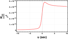
Figure 4: The evolution of memory observable $N_{\vartheta\vartheta}$ due to the passage of GW burst.

D.2 Amplification factor in Cosmological GW memory

Here, we aim to derive the form of the amplification factor. We begin by rewriting the relation between instantaneous memory and cumulative memory given in Eq.(4) for FLRW spacetime:

$$\partial_{\vartheta\vartheta}\left({N_{\vartheta\vartheta}}/{a^{2}}\right)={2\Sigma_{\vartheta\vartheta}}/{a}.$$ (61)

Considering that the burst profile traverses for a finite interval of conformal time ($\eta_{0},\eta_{1}$) and integrating Eq.(61) in that region, we obtain:

$$\left({N_{\vartheta\vartheta}}/{a^{2}}\right)\bigg{\rvert}_{\eta_{1}}-\left({N_{\vartheta\vartheta}}/{a^{2}}\right)\bigg{\rvert}_{\eta_{0}}=F(\eta_{1})-F(\eta_{0}),$$ (62)

where $F(\eta)=\int\frac{2\Sigma_{\vartheta\vartheta}}{a},d\eta$. Since the GW are massless, its energy density behaves as $(\frac{N_{+}}{a^{2}})^{2}$. Thus, to obtain the amplification of the GW memory amplitude, we compute the ratio of the quantity $(\frac{N_{+}}{a^{2}})$ at initial and final conformal times. We define amplification as:

$$A_{C}=\frac{\left({N_{\vartheta\vartheta}}/{a^{2}}\right)\rvert_{\eta_{1}}}{\left({N_{\vartheta\vartheta}}/{a^{2}}\right)\rvert_{\eta_{0}}}.$$

Plugging this relation back to Eq.(62) we get,

$$A_{C}=1+\dfrac{a^{2}(\eta_{0})}{h_{I}(\eta_{0})}\,[F(\eta_{1})-F(\eta_{0})].$$ (63)

Note at initial time $\eta_{i}$, $N_{\vartheta\vartheta}=h_{\vartheta\vartheta}^{I}(\eta_{0})$.

D.3 FLRW spacetime

We have previously discussed the amplification factor for matter domination (MD), dark energy (DE), and matter-to-$\Lambda$ transition. Here, we demonstrate how the amplification factor behaves for radiation-dominated (RD), and super-inflation (SI) scenarios [98, 99] for unit $e$-fold expansion.

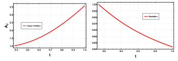
Figure 5: Evolution of the amplification factor for SI ($a(\eta)=1/(-\eta)^{1/20}$), and RD ($a(t)=t^{1/2}$).

Only in the case of SI do we observe an increase in amplification. In RD, we observe similar decaying features as were obtained for MD and DE phases.

References

- Weinberg [2008] S. Weinberg, Cosmology, Oxford Graduate Texts (Oxford University Press, 2008).
- Peter and Uzan [2013] P. Peter and J.-P. Uzan, Primordial Cosmology, Oxford Graduate Texts (Oxford University Press, 2013).
- Rees [2022] M. J. Rees, Ann. Rev. Astron. Astrophys. 60, 1 (2022).
- Melia [2022] F. Melia, Publ. Astron. Soc. Pac. 134, 121001 (2022).
- Ellis and Wands [2023] J. Ellis and D. Wands, (2023), arXiv:2312.13238 [astro-ph.CO] .
- Martin et al. [2014] J. Martin, C. Ringeval, and V. Vennin, Phys. Dark Univ. 5-6, 75 (2014), arXiv:1303.3787 [astro-ph.CO] .
- Odintsov et al. [2023] S. D. Odintsov, V. K. Oikonomou, I. Giannakoudi, F. P. Fronimos, and E. C. Lymperiadou, Symmetry 15, 1701 (2023), arXiv:2307.16308 [gr-qc] .
- Profumo et al. [2019] S. Profumo, L. Giani, and O. F. Piattella, Universe 5, 213 (2019), arXiv:1910.05610 [hep-ph] .
- Rajendran [2022] S. Rajendran, SciPost Phys. Lect. Notes 56, 1 (2022), arXiv:2204.03085 [hep-ph] .
- Carr and Kuhnel [2020] B. Carr and F. Kuhnel, Ann. Rev. Nucl. Part. Sci. 70, 355 (2020), arXiv:2006.02838 [astro-ph.CO] .
- Sahni and Starobinsky [2000] V. Sahni and A. A. Starobinsky, Int. J. Mod. Phys. D 9, 373 (2000), arXiv:astro-ph/9904398 .
- Peebles and Ratra [2003] P. J. E. Peebles and B. Ratra, Rev. Mod. Phys. 75, 559 (2003), arXiv:astro-ph/0207347 .
- Padmanabhan [2003] T. Padmanabhan, Phys. Rept. 380, 235 (2003), arXiv:hep-th/0212290 .
- Joyce et al. [2016] A. Joyce, L. Lombriser, and F. Schmidt, Ann. Rev. Nucl. Part. Sci. 66, 95 (2016), arXiv:1601.06133 [astro-ph.CO] .
- Motta et al. [2021] V. Motta, M. A. García-Aspeitia, A. Hernández-Almada, J. Magaña, and T. Verdugo, Universe 7, 163 (2021), arXiv:2104.04642 [astro-ph.CO] .
- Weinberg [1989] S. Weinberg, Rev. Mod. Phys. 61, 1 (1989).
- Weinberg [2000] S. Weinberg, in 4th International Symposium on Sources and Detection of Dark Matter in the Universe (DM 2000) (2000) pp. 18–26, arXiv:astro-ph/0005265 .
- Carroll [2001] S. M. Carroll, Living Rev. Rel. 4, 1 (2001), arXiv:astro-ph/0004075 .
- Di Valentino et al. [2021] E. Di Valentino, O. Mena, S. Pan, L. Visinelli, W. Yang, A. Melchiorri, D. F. Mota, A. G. Riess, and J. Silk, Class. Quant. Grav. 38, 153001 (2021), arXiv:2103.01183 [astro-ph.CO] .
- Shah et al. [2021] P. Shah, P. Lemos, and O. Lahav, Astron. Astrophys. Rev. 29, 9 (2021), arXiv:2109.01161 [astro-ph.CO] .
- Schöneberg et al. [2022] N. Schöneberg, G. Franco Abellán, A. Pérez Sánchez, S. J. Witte, V. Poulin, and J. Lesgourgues, Phys. Rept. 984, 1 (2022), arXiv:2107.10291 [astro-ph.CO] .
- Kamionkowski and Riess [2023] M. Kamionkowski and A. G. Riess, Ann. Rev. Nucl. Part. Sci. 73, 153 (2023), arXiv:2211.04492 [astro-ph.CO] .
- Shankaranarayanan and Johnson [2022] S. Shankaranarayanan and J. P. Johnson, Gen. Rel. Grav. 54, 44 (2022), arXiv:2204.06533 [gr-qc] .
- Lima et al. [2012] J. A. S. Lima, J. F. Jesus, R. C. Santos, and M. S. S. Gill, (2012), arXiv:1205.4688 [astro-ph.CO] .
- Moresco et al. [2016] M. Moresco, L. Pozzetti, A. Cimatti, R. Jimenez, C. Maraston, L. Verde, D. Thomas, A. Citro, R. Tojeiro, and D. Wilkinson, JCAP 05, 014 (2016), arXiv:1601.01701 [astro-ph.CO] .
- Sathyaprakash and Schutz [2009] B. S. Sathyaprakash and B. F. Schutz, Living Rev. Rel. 12, 2 (2009), arXiv:0903.0338 [gr-qc] .
- Sasaki et al. [2016] M. Sasaki, T. Suyama, T. Tanaka, and S. Yokoyama, Phys. Rev. Lett. 117, 061101 (2016), [Erratum: Phys.Rev.Lett. 121, 059901 (2018)], arXiv:1603.08338 [astro-ph.CO] .
- Bird et al. [2016] S. Bird, I. Cholis, J. B. Muñoz, Y. Ali-Haïmoud, M. Kamionkowski, E. D. Kovetz, A. Raccanelli, and A. G. Riess, Phys. Rev. Lett. 116, 201301 (2016), arXiv:1603.00464 [astro-ph.CO] .
- Hayasaki et al. [2016] K. Hayasaki, K. Takahashi, Y. Sendouda, and S. Nagataki, Publ. Astron. Soc. Jap. 68, 66 (2016), arXiv:0909.1738 [astro-ph.CO] .
- Abbott et al. [2017a] B. P. Abbott et al. (LIGO Scientific, Virgo, Fermi-GBM, INTEGRAL), Astrophys. J. Lett. 848, L13 (2017a), arXiv:1710.05834 [astro-ph.HE] .
- Abbott et al. [2017b] B. P. Abbott et al. (LIGO Scientific, Virgo), Phys. Rev. Lett. 119, 161101 (2017b), arXiv:1710.05832 [gr-qc] .
- de Rham and Melville [2018] C. de Rham and S. Melville, Phys. Rev. Lett. 121, 221101 (2018), arXiv:1806.09417 [hep-th] .
- Ezquiaga and Zumalacárregui [2017] J. M. Ezquiaga and M. Zumalacárregui, Phys. Rev. Lett. 119, 251304 (2017), arXiv:1710.05901 [astro-ph.CO] .
- Sakstein and Jain [2017] J. Sakstein and B. Jain, Phys. Rev. Lett. 119, 251303 (2017), arXiv:1710.05893 [astro-ph.CO] .
- Schutz [1986] B. F. Schutz, Nature 323, 310 (1986).
- Abbott et al. [2017c] B. P. Abbott et al. (LIGO Scientific, Virgo, 1M2H, Dark Energy Camera GW-E, DES, DLT40, Las Cumbres Observatory, VINROUGE, MASTER), Nature 551, 85 (2017c), arXiv:1710.05835 [astro-ph.CO] .
- Del Pozzo [2012] W. Del Pozzo, Phys. Rev. D 86, 043011 (2012), arXiv:1108.1317 [astro-ph.CO] .
- Nissanke et al. [2013] S. Nissanke, D. E. Holz, N. Dalal, S. A. Hughes, J. L. Sievers, and C. M. Hirata, (2013), arXiv:1307.2638 [astro-ph.CO] .
- Braginsky and Grishchuk [1985] V. B. Braginsky and L. P. Grishchuk, Sov. Phys. JETP 62, 427 (1985).
- Favata [2010] M. Favata, Class. Quant. Grav. 27, 084036 (2010), arXiv:1003.3486 [gr-qc] .
- Zel’dovich and Polnarev [1974] Y. B. Zel’dovich and A. G. Polnarev, Sov. Astron. 18, 17 (1974).
- Christodoulou [1991] D. Christodoulou, Phys. Rev. Lett. 67, 1486 (1991).
- Braginskii and Thorne [1987] V. B. Braginskii and K. S. Thorne, Nature 327, 123 (1987).
- Favata [2009] M. Favata, Astrophys. J. Lett. 696, L159 (2009), arXiv:0902.3660 [astro-ph.SR] .
- Zhang et al. [2017] P. M. Zhang, C. Duval, G. W. Gibbons, and P. A. Horvathy, Phys. Rev. D 96, 064013 (2017), arXiv:1705.01378 [gr-qc] .
- Strominger and Zhiboedov [2016a] A. Strominger and A. Zhiboedov, JHEP 01, 086 (2016a), arXiv:1411.5745 [hep-th] .
- Flanagan and Nichols [2017] E. E. Flanagan and D. A. Nichols, Phys. Rev. D 95, 044002 (2017), [Erratum: Phys.Rev.D 108, 069902 (2023)], arXiv:1510.03386 [hep-th] .
- Nichols [2017] D. A. Nichols, Phys. Rev. D 95, 084048 (2017), arXiv:1702.03300 [gr-qc] .
- Mitman et al. [2020] K. Mitman, J. Moxon, M. A. Scheel, S. A. Teukolsky, M. Boyle, N. Deppe, L. E. Kidder, and W. Throwe, Phys. Rev. D 102, 104007 (2020), arXiv:2007.11562 [gr-qc] .
- Strominger [2017] A. Strominger, Lectures on the Infrared Structure of Gravity and Gauge Theory (2017) arXiv:1703.05448 [hep-th] .
- Compère and Fiorucci [2018] G. Compère and A. Fiorucci, (2018), arXiv:1801.07064 [hep-th] .
- Thorne [1992] K. S. Thorne, Phys. Rev. D 45, 520 (1992).
- Wiseman and Will [1991] A. G. Wiseman and C. M. Will, Phys. Rev. D 44, R2945 (1991).
- Jenkins and Sakellariadou [2021] A. C. Jenkins and M. Sakellariadou, Class. Quant. Grav. 38, 165004 (2021), arXiv:2102.12487 [gr-qc] .
- Mukhopadhyay et al. [2021] M. Mukhopadhyay, C. Cardona, and C. Lunardini, JCAP 07, 055 (2021), arXiv:2105.05862 [astro-ph.HE] .
- Jokela et al. [2022] N. Jokela, K. Kajantie, and M. Sarkkinen, Phys. Rev. D 106, 064022 (2022), arXiv:2204.06981 [gr-qc] .
- Shore [2018] G. M. Shore, JHEP 12, 133 (2018), arXiv:1811.08827 [gr-qc] .
- Siddhant et al. [2021] S. Siddhant, I. Chakraborty, and S. Kar, Eur. Phys. J. C 81, 350 (2021), arXiv:2011.12368 [gr-qc] .
- Chakraborty [2022] I. Chakraborty, Phys. Rev. D 105, 024063 (2022), arXiv:2110.02295 [gr-qc] .
- Heisenberg et al. [2023] L. Heisenberg, N. Yunes, and J. Zosso, Phys. Rev. D 108, 024010 (2023), arXiv:2303.02021 [gr-qc] .
- Tolish and Wald [2016] A. Tolish and R. M. Wald, Phys. Rev. D 94, 044009 (2016), arXiv:1606.04894 [gr-qc] .
- Bieri et al. [2017] L. Bieri, D. Garfinkle, and N. Yunes, Class. Quant. Grav. 34, 215002 (2017), arXiv:1706.02009 [gr-qc] .
- Chu [2017] Y.-Z. Chu, Class. Quant. Grav. 34, 035009 (2017), arXiv:1603.00151 [gr-qc] .
- Kehagias and Riotto [2016] A. Kehagias and A. Riotto, JCAP 05, 059 (2016), arXiv:1602.02653 [hep-th] .
- Jana and Shankaranarayanan [2023] S. Jana and S. Shankaranarayanan, Phys. Rev. D 108, 024044 (2023), arXiv:2301.11772 [gr-qc] .
- van Elst and Ellis [1996] H. van Elst and G. F. R. Ellis, Class. Quant. Grav. 13, 1099 (1996), arXiv:gr-qc/9510044 .
- Ellis [1967] G. F. R. Ellis, J. Math. Phys. 8, 1171 (1967).
- Clarkson et al. [2004] C. A. Clarkson, M. Marklund, G. Betschart, and P. K. S. Dunsby, Astrophys. J. 613, 492 (2004), arXiv:astro-ph/0310323 .
- Clarkson and Barrett [2003] C. A. Clarkson and R. K. Barrett, Class. Quant. Grav. 20, 3855 (2003), arXiv:gr-qc/0209051 .
- Clarkson [2007] C. Clarkson, Phys. Rev. D 76, 104034 (2007), arXiv:0708.1398 [gr-qc] .
- Goswami and Ellis [2021] R. Goswami and G. F. R. Ellis, Class. Quant. Grav. 38, 085023 (2021), arXiv:1912.00591 [gr-qc] .
- Owen et al. [2011a] R. Owen et al., Phys. Rev. Lett. 106, 151101 (2011a), arXiv:1012.4869 [gr-qc] .
- Zhang et al. [2012] F. Zhang, A. Zimmerman, D. A. Nichols, Y. Chen, G. Lovelace, K. D. Matthews, R. Owen, and K. S. Thorne, Phys. Rev. D 86, 084049 (2012), arXiv:1208.3034 [gr-qc] .
- Maartens and Bassett [1998] R. Maartens and B. A. Bassett, Class. Quant. Grav. 15, 705 (1998), arXiv:gr-qc/9704059 .
- Herrera et al. [2006] L. Herrera, N. O. Santos, and J. Carot, J. Math. Phys. 47, 052502 (2006), arXiv:gr-qc/0511112 .
- Bruni et al. [1992] M. Bruni, P. K. S. Dunsby, and G. F. R. Ellis, Astrophys. J. 395, 34 (1992).
- Ellis et al. [2012] G. F. R. Ellis, R. Maartens, and M. A. H. MacCallum, Relativistic Cosmology (Cambridge University Press, 2012).
- Bieri and Garfinkle [2014] L. Bieri and D. Garfinkle, Phys. Rev. D 89, 084039 (2014), arXiv:1312.6871 [gr-qc] .
- Tolish et al. [2014] A. Tolish, L. Bieri, D. Garfinkle, and R. M. Wald, Phys. Rev. D 90, 044060 (2014), arXiv:1405.6396 [gr-qc] .
- Strominger and Zhiboedov [2016b] A. Strominger and A. Zhiboedov, JHEP 01, 086 (2016b), arXiv:1411.5745 [hep-th] .
- Kovacs and Thorne [1978] S. J. Kovacs and K. S. Thorne, Astrophys. J. 224, 62 (1978).
- Trashorras et al. [2021] M. Trashorras, J. García-Bellido, and S. Nesseris, Universe 7, 18 (2021), arXiv:2006.15018 [astro-ph.CO] .
- De Vittori et al. [2012] L. De Vittori, P. Jetzer, and A. Klein, Phys. Rev. D 86, 044017 (2012), arXiv:1207.5359 [gr-qc] .
- Mukherjee et al. [2021] S. Mukherjee, S. Mitra, and S. Chatterjee, Mon. Not. Roy. Astron. Soc. 508, 5064 (2021), arXiv:2010.00916 [gr-qc] .
- Nichols et al. [2011] D. A. Nichols et al., Phys. Rev. D 84, 124014 (2011), arXiv:1108.5486 [gr-qc] .
- Mavrogiannis and Tsagas [2021] P. Mavrogiannis and C. G. Tsagas, Phys. Rev. D 104, 124053 (2021), arXiv:2110.02489 [gr-qc] .
- Riess et al. [1998] A. G. Riess et al. (Supernova Search Team), Astron. J. 116, 1009 (1998), arXiv:astro-ph/9805201 .
- Perlmutter et al. [1999] S. Perlmutter et al. (Supernova Cosmology Project), Astrophys. J. 517, 565 (1999), arXiv:astro-ph/9812133 .
- Eisenstein et al. [2005] D. J. Eisenstein et al. (SDSS), Astrophys. J. 633, 560 (2005), arXiv:astro-ph/0501171 .
- Aghanim et al. [2020] N. Aghanim et al. (Planck), Astron. Astrophys. 641, A6 (2020), [Erratum: Astron.Astrophys. 652, C4 (2021)], arXiv:1807.06209 [astro-ph.CO] .
- Capozziello et al. [2014] S. Capozziello, O. Farooq, O. Luongo, and B. Ratra, Phys. Rev. D 90, 044016 (2014), arXiv:1403.1421 [gr-qc] .
- Capozziello et al. [2015] S. Capozziello, O. Luongo, and E. N. Saridakis, Phys. Rev. D 91, 124037 (2015), arXiv:1503.02832 [gr-qc] .
- Ellis and van Elst [1999] G. F. R. Ellis and H. van Elst, NATO Sci. Ser. C 541, 1 (1999), arXiv:gr-qc/9812046 .
- Heckmann and Schucking [1955] O. Heckmann and E. Schucking, zap 38, 95 (1955).
- Raychaudhuri [1955] A. Raychaudhuri, Physical Review 98, 1123 (1955).
- Hawking [1966] S. W. Hawking, Astrophys. J. 145, 544 (1966).
- Owen et al. [2011b] R. Owen et al., Phys. Rev. Lett. 106, 151101 (2011b), arXiv:1012.4869 [gr-qc] .
- Biswas and Mazumdar [2014] T. Biswas and A. Mazumdar, Class. Quant. Grav. 31, 025019 (2014), arXiv:1304.3648 [hep-th] .
- Basak and Shankaranarayanan [2015] A. Basak and S. Shankaranarayanan, JCAP 05, 034 (2015), arXiv:1410.5768 [hep-ph] .