Improved uniform error bounds for long-time dynamics of the high-dimensional nonlinear space fractional sine-Gordon equation with weak nonlinearity

Abstract

In this paper, we derive the improved uniform error bounds for the long-time dynamics of the $d$-dimensional $(d=2,3)$ nonlinear space fractional sine-Gordon equation (NSFSGE). The nonlinearity strength of the NSFSGE is characterized by $\varepsilon^{2}$ where $0<\varepsilon\leq 1$ is a dimensionless parameter. The second-order time-splitting method is applied to the temporal discretization and the Fourier pseudo-spectral method is used for the spatial discretization. To obtain the explicit relation between the numerical errors and the parameter $\varepsilon$, we introduce the regularity compensation oscillation technique to the convergence analysis of fractional models. Then we establish the improved uniform error bounds $O\left(\varepsilon^{2}\tau^{2}\right)$ for the semi-discretization scheme and $O\left(h^{m}+\varepsilon^{2}\tau^{2}\right)$ for the full-discretization scheme up to the long time at $O(1/\varepsilon^{2})$. Further, we extend the time-splitting Fourier pseudo-spectral method to the complex NSFSGE as well as the oscillatory complex NSFSGE, and the improved uniform error bounds for them are also given. Finally, extensive numerical examples in two-dimension or three-dimension are provided to support the theoretical analysis. The differences in dynamic behaviors between the fractional sine-Gordon equation and classical sine-Gordon equation are also discussed.

1 Introduction

Nonlinear wave equations and their dynamic properties explain the rich and colorful natural phenomena reasonably, such as the wave propagation, smooth scattering, emission and absorption in electromagnetism, superelastic material [1, 2, 3, 4]. Some well-known nonlinear wave equations are Schrödinger equations, Klein-Gordon equations, sine-Gordon equations, Korteweg-deVries equation, Burgers equation and so on. As an important class of nonlinear hyperbolic equations, the sine-Gordon equation has many soliton solutions. So it is widely used in biophysics, fluid motion, quantum mechanics, nonlinear media super transport, plasma physics and other scientific fields [5]. A lot of studies have been done for the analytical analysis and numerical research on the soliton solutions of the sine-Gordon [6, 7, 8].

In classical nonlinear partial differential equations, the state of a point is directly affected by its nearest points. However, in many practical physical phenomena, the state of one point can be affected by points farther away, which is called the non-locality and remote correlation. Considering that fractional operators have nonlocality and memory properties, fractional models have great advantages in describing the above phenomena. Some studies have shown that space fractional models can relatively accurately describe complex phenomena such as anomalous diffusion transport, remote interactions and fractal dispersion [9, 10]. In this view, more and more classical models have been expressed in fractional systems [11, 12, 13, 14]. The space fractional sine-Gordon equation is an extension of the classical sine-Gordon equation, which is an important dynamic model with remote interactions in nonlinear science [15, 16, 17]. For instance, Korabel et al. [16] discovered the soliton-like and breather-like patterns of the fractional sine-Gordon equation. Macías-Díaz [17] numerically proved the existence of nonlinear supertransmission in the space fractional sine-Gordon system.

In this paper, we consider the following high-dimensional nonlinear space fractional sine-Gordon equation (NSFSGE)

$$\left\{\begin{array}[]{l}\partial_{tt}\psi(\mathbf{x},t)+(-\Delta)^{\alpha/2}\psi(\mathbf{x},t)+\sin(\psi(\mathbf{x},t))=0,\quad\mathbf{x}\in\Omega,\quad t>0,\\ \psi(\mathbf{x},0)=\varepsilon\psi_{0}(\mathbf{x}),\quad\partial_{t}\psi(\mathbf{x},0)=\varepsilon\psi_{1}(\mathbf{x}),\quad\mathbf{x}\in\bar{\Omega},\end{array}\right.$$ (1)

with periodic boundary conditions. $\psi:=\psi(\mathbf{x},t)$ is a real-valued function, $\mathbf{x}$ is the spatial coordinate, $t$ is the time variable, and $\Omega=\prod_{i=1}^{d}(a_{i},b_{i})\subset\mathbb{R}^{d}(d=2,3)$ is a compact domain. $\psi_{0}(\mathbf{x})$, $\psi_{1}(\mathbf{x})$ are two known real initial functions independent of $\varepsilon$. $\varepsilon\in(0,1]$ is a dimensionless parameter to depict the nonlinearity strength of Eq. (1). $(-\Delta)^{{}^{\alpha/2}}(1<\alpha\leq 2)$ is the space fractional Laplacian, which is defined by [18, 19]

$$(-\Delta)^{{}^{\alpha/2}}\psi(\mathbf{x},t)=\mathscr{F}^{-1}\left(|\bm{\omega}|^{\alpha}\widehat{\psi}(\bm{\omega},t)\right),\quad\widehat{\psi}(\bm{\omega},t)=\mathscr{F}\psi(\bm{\omega},t),$$

where $\bm{\omega}$ is the $d$-dimensional vector, $\mathscr{F}(\psi)$ denotes the Fourier transform of $z$ and $\mathscr{F}^{-1}$ stands for its inverse transform. Considering that $\Omega$ is a bounded domain, the fractional Laplace operator $(-\Delta)^{{}^{\alpha/2}}(1<\alpha\leq 2)$ can be defined by finite Fourier series as [20, 21]

$$(-\Delta)^{{}^{\alpha/2}}\psi(\mathbf{x},t)=\sum_{\mathbf{k}\in\mathbb{Z}^{d}}|\mu\mathbf{k}|^{\alpha}\widehat{\psi}_{\mathbf{k}}\mathrm{e}^{i\mu\mathbf{k}(\mathbf{x}-a)},$$

here $i$ is the imaginary unit, $|\mu\mathbf{k}|^{\alpha}=(\sum_{i=1}^{d}\left|\mu_{i}\right|^{2})^{\alpha/2}$, $\mu\mathbf{k}(\mathbf{x}-a)=\sum_{i=1}^{d}\mu_{i}(x_{i}-a_{i})$, $\mu_{i}=\frac{2\pi k_{i}}{b_{i}-a_{i}}$, where $x_{i}$, $k_{i}$ represent the component of $\mathbf{x}$, $\mathbf{k}$, respectively. The Fourier coefficients can be given as

$$\widehat{\psi}_{\mathbf{k}}=\frac{1}{\prod_{i=1}^{d}(b_{i}-a_{i})}\int_{\Omega}\psi(\mathbf{x},t)\mathrm{e}^{-i\mu\mathbf{k}(\mathbf{x}-a)}d\mathbf{x}.$$

When $\alpha=2$, the NSFSGE (1) is reduced to the classical sine-Gordon equation.

When $0<\varepsilon\ll 1$, we introduce $u(\mathbf{x},t)=\psi(\mathbf{x},t)/\varepsilon$. The NSFSGE (1) with $O(\varepsilon)$ initial data and $O(1)$ nonlinearity can be turned to the following NSFSGE:

$$\left\{\begin{array}[]{l}\partial_{tt}u(\mathbf{x},t)+(-\Delta)^{\alpha/{2}}u(\mathbf{x},t)+\frac{1}{\varepsilon}\sin(\varepsilon u(\mathbf{x},t))=0,\quad\mathbf{x}\in\Omega,\quad t>0,\\ u(\mathbf{x},0)=u_{0}(\mathbf{x}),\quad\partial_{t}u(\mathbf{x},0)=u_{1}(\mathbf{x}),\quad\mathbf{x}\in\bar{\Omega}.\end{array}\right.$$ (2)

where $u_{0}(\mathbf{x})=\psi_{0}(\mathbf{x})$, $u_{1}(\mathbf{x})=\psi_{1}(\mathbf{x})$. For Eq. (2), we use the Taylor expansion $\sin(u)=u-\frac{u^{3}}{6}+O(u^{5})$ and give the leading order behevior of the solution is

$$\partial_{tt}u(\mathbf{x},t)+(-\Delta)^{\alpha/{2}}u(\mathbf{x},t)+u(\mathbf{x},t)-\frac{\varepsilon^{2}u^{3}(\mathbf{x},t)}{6}=0,$$ (3)

which shows the lifespan of Eq. (2) is at least up to $O(1/\varepsilon^{2})$ according to the research for the nonlinear Klein-Gordon equation provided with the cubic nonlinearlity [22, 23]. Note that the long-time dynamics of the NSFSGE (1) is equivalent to that of the NSFSGE (2). Then we only discuss the error estimation of the long-time dynamics for the NSFSGE (2) with weak nonlinearity at time $O(1/\varepsilon^{2})$ and the relevant conclusions can be easily generalized to Eq. (1).

When $\varepsilon=1$, the NSFSGE (2) is in the standard classical regime and there are many numerical studies for it [15, 21, 24, 25, 26]. Ran and Zhang [25] proposed a compact difference scheme with convergence accuracy of fourth-order in space and second-order in time to solve the NSFSGE. Alfimov et al. [26] numerically explored the breather-like solution of the NSFSGE by using the rotating wave approximation method. A dissipation-preserving Fourier pseudo-spectral method was given for the NSFSGE with damping in [21]. Fu et al. [15] proposed a linearly implicit structure-preserving numerical scheme for the NSFSGE, in which the stability and convergence in the maximum norm of the numerical scheme were given. However, those numerical method and error estimation are generally effective up to the time at $O(1)$. When $0<\varepsilon\ll 1$, the lifespan of the solution for the NSFSGE (2) is up to the time at $O(1/\varepsilon^{2})$. An important work is to extend those classical error bounds for the NSFSGE (2) up to the time at $O(1/\varepsilon^{2})$ instead of $O(1)$, i.e., the long-time error analysis.

The long-time dynamics of the classical nonlinear equation with weak nonlinearity has attracted much attention [27, 28, 29, 30, 31, 32]. Cohen et al. [30] used a modulated Fourier expansion to carry out the long-time analysis of the nonlinearly perturbed wave equations. Bao et al. [28] established improved uniform error bounds on a second-order time-splitting method for the nonlinear Schrödinger equation up to time at $O(1/\varepsilon^{2})$ by introducing a new technique of regularity compensation oscillation. The paper [31] presented the long time error analysis of the fourth-order compact finite difference methods for the nonlinear Klein-Gordon equation. An exponential wave integrator Fourier pseudo-spectral method for the long-time dynamics of the nonlinear Klein-Gordon equation was developed in [32]. As far as we know, the existing research on long-time dynamics is focused on integer equations and there is limited research on long-time dynamics of nonlinear fractional equations. For the long-time dynamics of nonlinear fractional wave equations, the behaviors of the plane wave solutions are significantly different from that of classical equations and the fractional order can affect the width and height of the solution [33, 34]. So it is an interesting and challenging research topic for proposing an effective numerical method and error estimation for long-time nonlinear fractional models.

The aim of this paper is to obtain the improved uniform error bounds in $H^{\alpha/2}$-norm of the high-dimensional NSFSGE (2) up to the time at $T_{\varepsilon}=T/\varepsilon^{2}$ with $T$ fixed. The inherent differences in dynamic behaviors between the fractional sine-Gordon equation and classical sine-Gordon equation are discussed. The difficulties are the numerical analysis of fractional operators and how to give the explicit dependence of the errors and the parameter $\varepsilon$ in fractional equations. The main contributions of this paper can be listed as

$\bullet$ To obtain the uniform error bounds for the long-time dynamics, one of the tricks used here is that a linear part from the sine function of the NSFSGE is separated. Then we transform the NSFSGE to an equivalent relativistic nonlinear space fractional Schrödinger equation (NSFSE). With the help of the Strang splitting technique [35, 36], we decompose the NSFSE into a linear equation and a nonlinear equation, and the second-order time-splitting Fourier pseudo-spectral method is developed.

$\bullet$ We introduce the regularity compensation oscillation technique to the convergence analysis of fractional models, which the high-frequency modes are controlled by regularity and the low-frequency modes are analyzed by phase cancellation as well as energy method, then we give the improved uniform error bounds $O\left(\varepsilon^{2}\tau^{2}\right)$ for the semi-discretization scheme and $O\left(h^{m}+\varepsilon^{2}\tau^{2}\right)$ for the full-discretization scheme. The explicit relation of the errors and the parameter $\varepsilon$ is specified.

$\bullet$ Compared with the existing references [29, 37], we prove the error bounds for the fully discretization directly by the mathematical induction without comparing with the semi-discretization in time, so the bound of the semi-discrete numerical solution $\lVert\varphi^{[n]}\rVert_{H^{m+\alpha/2}}$ is not needed in this paper.

The organization of this paper is as follows. In Section 2, we give some notation and use a second-order time-splitting Fourier pseudo-spectral method to obtain the numerical scheme of the NSFSGE (2). Section 3 gives the improved uniform error bounds for the semi-discretization scheme and full discretization scheme by the regularity compensation oscillation technique, respectively. In Section 4, we extend the time-splitting Fourier pseudo-spectral method and corresponding error bounds to the complex NSFSGE as well as the oscillatory complex NSFSGE. Section 5 verifies the validity of the numerical scheme and error bounds through some specific examples. Finally, we give some conclusions in Section 6.

2 Numerical method

For convenience, we only give the numerical scheme and error estimation for the NSFSGE (2) in the two-dimension (2D). It is similar for the NSFSGE (2) in the three-dimension (3D). In 2D, we further assume $\Omega=(a,b)^{2}$ for simplification, Eq. (2) with periodic boundary conditions can be expressed as

$$\left\{\begin{array}[]{l}\partial_{tt}u(x,y,t)+(-\Delta)^{\alpha/2}u(x,y,t)+\frac{1}{\varepsilon}\sin(\varepsilon u(x,y,t))=0,\quad(x,y)\in\Omega,\quad t>0,\\ u(x,y,0)=u_{0}(x,y),\quad\partial_{t}u(x,y,0)=u_{1}(x,y),\quad(x,y)\in\bar{\Omega}.\end{array}\right.$$ (4)

In the remainder of this paper, let $C>0$ denote positive constants independent of the time step $\tau$, the space step $h$ and $\varepsilon$. The notation $A\lesssim B$ is adopted to denote $|A|\leq CB$.

2.1 Preliminary

Let $L^{2}(\Omega)$ be the standard $L^{2}$-space, $C_{per}(\Omega)=\{u\in C(\bar{\Omega})\mid\text{$u$ is periodic}\}$ and

$$Y_{N}:=\operatorname{span}\left\{\mathrm{e}^{i\mu_{k}(x-a)+i\mu_{l}(y-a)}:\mu_{j}=\frac{2\pi j}{b-a},k,l\in T_{N}\right\},$$

$$T_{N}=\left\{j\mid j=-\frac{N}{2},-\frac{N}{2}+1,\ldots,\frac{N}{2}-1\right\},$$

here $N$ is an even positive integer. Denote $P_{N}:L^{2}(\Omega)\rightarrow Y_{N}$ as the standard $L^{2}$-projection operator, $I_{N}:C_{per}(\Omega)\rightarrow Y_{N}$ as the trigonometric interpolation operator, i.e.,

$$P_{N}u(x,y)=\sum_{k,l\in T_{N}}\widehat{u}_{kl}\mathrm{e}^{i\mu_{k}(x-a)+i\mu_{l}(y-a)},\quad I_{N}u(x,y)=\sum_{k,l\in T_{N}}\tilde{u}_{kl}\mathrm{e}^{i\mu_{k}(x-a)+i\mu_{l}(y-a)},\quad(x,y)\in\bar{\Omega},$$

where

$$\widehat{u}_{kl}=\frac{1}{(b-a)^{2}}\int_{\Omega}u(x,y)\mathrm{e}^{-i\mu_{k}(x-a)-i\mu_{l}(y-a)}{d}{\Omega},\quad\tilde{u}_{kl}=\frac{1}{N^{2}}\sum_{p=0}^{N-1}\sum_{q=0}^{N-1}u_{pq}\mathrm{e}^{-i\mu_{k}\left(x_{p}-a\right)-i\mu_{l}\left(y_{q}-a\right)},$$

and $u_{pq}$ is defined as $u\left(x_{p},y_{q}\right)$.

For $m\geq 0,H^{m}(\Omega)$ is the space of functions $u(x,y)\in L^{2}(\Omega)$, the $H^{m}$-norm $\|\cdot\|_{m}$ is defined by

$$\|u\|_{m}^{2}=\sum_{k,l\in\mathbb{Z}}\left(1+\left|\mu_{k}\right|^{2}+\left|\mu_{l}\right|^{2}\right)^{m}\left|\widehat{u}_{kl}\right|^{2},\quad\text{ for }\quad u(x,y)=\sum_{k,l\in\mathbb{Z}}\widehat{u}_{kl}\mathrm{e}^{i\mu_{k}(x-a)+i\mu_{l}(y-a)},$$

where $\widehat{u}_{kl}(k,l\in\mathbb{Z})$ denotes the Fourier coefficients of $u(x,y)$. Furthermore, $H^{0}(\Omega)=$ $L^{2}(\Omega)$ and $\|\cdot\|$ denotes the $L^{2}-$norm $\|\cdot\|_{0}$. We denote $L^{\infty}([0,T];H^{m}(\Omega))$ with $T>0$ as the space of the functions $u:[0,T]\to H^{m}(\Omega)$ such that

$$\lVert u\rVert_{L^{\infty}([0,T];H^{m}(\Omega))}=\mathop{esssup}\limits_{0\leq t\leq T}\lVert u(t)\rVert_{m}<+\infty.$$

Define the operator $\langle\nabla\rangle_{\alpha}=\sqrt{1+(-\Delta)^{{\alpha}/{2}}}$ as

$$\langle\nabla\rangle_{\alpha}u(x,y)=\sum_{k,l\in\mathbb{Z}}\sqrt{1+\left(\left|\mu_{k}\right|^{2}+\left|\mu_{l}\right|^{2}\right)^{\alpha/2}}\widehat{u}_{kl}\mathrm{e}^{i\mu_{k}(x-a)+i\mu_{l}(y-a)}$$

and the inverse operator $\langle\nabla\rangle_{\alpha}^{-1}$ as

$$\langle\nabla\rangle_{\alpha}^{-1}u(x,y)=\sum_{k,l\in\mathbb{Z}}\frac{\widehat{u}_{kl}}{\sqrt{1+\left(\left|\mu_{k}\right|^{2}+\left|\mu_{l}\right|^{2}\right)^{\alpha/2}}}\mathrm{e}^{i\mu_{k}(x-a)+i\mu_{l}(y-a)}.$$

It is easy to get

$$\left\|\langle\nabla\rangle_{\alpha}^{-1}u\right\|_{s}\lesssim\|u\|_{s-\alpha/2}\lesssim\|u\|_{s},\quad\left\|\langle\nabla\rangle_{\alpha}u\right\|_{s}\lesssim\|u\|_{s+\alpha/2}\lesssim\|u\|_{s+1}.$$

For Eq. (4), we first separate a linear part $u(x,y,t)$ from $\frac{1}{\varepsilon}\sin({\varepsilon u(x,y,t)})$ and get

$$\partial_{tt}u(x,y,t)+\langle\nabla\rangle_{{\alpha}}^{2}u(x,y,t)+\frac{1}{\varepsilon}\sin(\varepsilon u(x,y,t))-u(x,y,t)=0,\quad(x,y)\in\Omega,\quad t>0.$$ (5)

Introducing $v(x,y,t)=\partial_{t}u(x,y,t)$ and $\varphi(x,y,t)=u(x,y,t)-i\langle\nabla\rangle_{\alpha}^{-1}v(x,y,t)$, we can get $\partial_{t}v(x,y,t)=i\langle\nabla\rangle_{\alpha}\partial_{t}\varphi(x,y,t)-i\langle\nabla\rangle_{\alpha}v(x,y,t)$ and $u(x,y,t)=\varphi(x,y,t)-i\langle\nabla\rangle_{\alpha}^{-1}v(x,y,t)$. Then Eq. (5) is equivalent to the following nonlinear space fractional Schrödinger equation (NSFSE) with periodic boundary conditions:

$$\left\{\begin{array}[]{lll}i\partial_{t}\varphi(x,y,t)+\langle\nabla\rangle_{\alpha}\varphi(x,y,t)+\langle\nabla\rangle_{\alpha}^{-1}f(\frac{\varphi+\bar{\varphi}}{2})(x,y,t)=0,&(x,y)\in\Omega,\quad t>0,\\ \varphi(x,y,0)=\varphi_{0}(x,y):=u_{0}(x,y)-i\langle\nabla\rangle^{-1}u_{1}(x,y),\quad(x,y)\in\bar{\Omega},\end{array}\right.$$ (6)

where $f(u)=\frac{1}{\varepsilon}\sin(\varepsilon u(x,y,t))-u(x,y,t)$, $\bar{\varphi}$ is the complex conjugate of $\varphi$. Note that the solution of Eq. (4) is

$$u(x,y,t)=\frac{1}{2}(\varphi(x,y,t)+\bar{\varphi}(x,y,t)),\quad v(x,y,t)=\frac{i}{2}\langle\nabla\rangle_{\alpha}(\varphi(x,y,t)-\bar{\varphi}(x,y,t)).$$ (7)

2.2 Numerical scheme

By the Strang splitting technique, the relativistic NSFSE (6) can be decomposed into a linear part and a nonlinear part. The linear part is

$$\left\{\begin{array}[]{l}\partial_{t}\varphi(x,y,t)=i\langle\nabla\rangle_{\alpha}\varphi(x,y,t),\\ \varphi(x,y,0)=\varphi_{0}(x,y),\end{array}\right.$$ (8)

and it can be solved exactly in phase space as

$$\varphi(x,y,t)=\phi_{T}^{t}(\varphi_{0})=\mathrm{e}^{it\langle\nabla\rangle_{\alpha}}\varphi_{0}(x,y),\quad t\geq 0.$$ (9)

The nonlinear part is

$$\left\{\begin{array}[]{l}\partial_{t}\varphi(x,y,t)=F(\varphi(x,y,t)),\\ \varphi(x,y,0)=\varphi_{0}(x,y),\end{array}\right.$$ (10)

where the nonlinear operator $F$ has the following expression

$$F(\varphi)=i\langle\nabla\rangle_{\alpha}^{-1}f(\frac{\varphi+\bar{\varphi}}{2}),\quad f(\frac{\varphi+\bar{\varphi}}{2})=\frac{1}{\varepsilon}\sin(\frac{\varepsilon(\varphi+\bar{\varphi})}{2})-\frac{\varphi+\bar{\varphi}}{2}.$$

Then (10) can be integrated exactly in time as

$$\varphi(x,y,t)=\phi_{V}^{t}(\varphi_{0})=\varphi_{0}(x,y)+tF(\varphi_{0}(x,y)),\quad t\geq 0.$$ (11)

Let $\tau>0$ denote the time step and $t_{n}:=n\tau,n=0,1,2,\cdots.$ We define $\varphi^{[n]}:=\varphi^{[n]}(x,y)$ as the time numerical approximation of $\varphi\left(x,y,t_{n}\right)$. Based on the Strang splitting, the second-order time-splitting method for the relativistic NSFSE (6) can be given as

$$\varphi^{[n+1]}=S_{\tau}(\varphi^{[n]})=\phi_{T}^{\frac{\tau}{2}}\circ\phi_{V}^{\tau}\circ\phi^{\frac{\tau}{2}}_{T}(\varphi^{[n]})=\mathrm{e}^{i\tau\langle\nabla\rangle_{\alpha}}\varphi^{[n]}+\tau\mathrm{e}^{i\frac{\tau\langle\nabla\rangle_{\alpha}}{2}}F\left(\mathrm{e}^{i\frac{\tau\langle\nabla\rangle_{\alpha}}{2}}\varphi^{[n]}\right),$$ (12)

and $\varphi^{[0]}=\varphi_{0}=u_{0}-i\langle\nabla\rangle_{\alpha}^{-1}u_{1}$. Hence the time discrete scheme for Eq. (2) is

$$u^{[n+1]}=\frac{1}{2}\left(\varphi^{[n+1]}+\overline{\varphi^{[n+1]}}\right),\quad v^{[n+1]}=\frac{i}{2}\langle\nabla\rangle_{\alpha}\left(\varphi^{[n+1]}-\overline{\varphi^{[n+1]}}\right),\quad n=0,1,\ldots,$$ (13)

with $u^{[0]}=u_{0}(x,y)$ and $v^{[0]}=u_{1}(x,y)$. Here, $u^{[n]}:=u^{[n]}(x,y)$ and $v^{[n]}:=v^{[n]}(x,y)$ are the numerical approximations of $u\left(x,y,t_{n}\right)$ and $v\left(x,y,t_{n}\right)$, respectively.

Next, we use the Fourier pseudo-spectral method [38] for the spatial approximation. Let $h=(b-a)/N$ be the space step. The grid points are denoted as $x_{p}:=a+ph,\quad y_{q}:=a+qh,\quad p,q=0,1,2,\cdots,N.$ Denote $\varphi_{pq}^{n}$ as the numerical approximation of $\varphi\left(x_{p},y_{q},t_{n}\right)$, $\varphi^{n}=\left(\varphi_{00}^{n},\varphi_{10}^{n},\ldots,\varphi_{N0}^{n},\ldots,\varphi_{0N}^{n},\ldots,\varphi_{NN}^{n},\right)^{T}\in\mathbb{C}^{(N+1)\times(N+1)}$, where $\varphi_{0q}^{n}=\varphi_{Nq}^{n}=\varphi_{p0}^{n}=\varphi_{pN}^{n}$, then a time-splitting Fourier pseudo-spectral (TSFP) method for (6) is

$$\begin{split}\varphi_{pq}^{(1)}&=\sum_{k,l\in T_{N}}\mathrm{e}^{i\frac{\tau\delta_{kl}}{2}}(\widetilde{\varphi^{n}})_{kl}\mathrm{e}^{i\mu_{k}\left(x_{p}-a\right)+i\mu_{l}\left(y_{q}-a\right)},\\ \varphi_{pq}^{(2)}&=\varphi_{pq}^{(1)}+\tau F_{pq}^{n},\quad F_{pq}^{n}=\sum_{k,l\in T_{N}}\frac{i}{\delta_{kl}}\left(\widetilde{f(\frac{\varphi^{(1)}+\overline{\varphi^{(1)}}}{2})}\right)_{kl}\mathrm{e}^{i\mu_{k}\left(x_{p}-a\right)+i\mu_{l}\left(y_{q}-a\right)},\\ \varphi_{pq}^{n+1}&=\sum_{k,l\in T_{N}}\mathrm{e}^{i\frac{\tau\delta_{kl}}{2}}(\widetilde{\varphi^{(2)}})_{kl}\mathrm{e}^{i\mu_{k}\left(x_{p}-a\right)+i\mu_{l}\left(y_{q}-a\right)},\end{split}$$ (14)

with $\varphi_{pq}^{0}=u_{0}\left(x_{p},y_{q}\right)-i\sum\limits_{k,l\in T_{N}}\frac{\widetilde{\left(u_{1}\right)_{kl}}}{\delta_{kl}}\mathrm{e}^{i\mu_{k}\left(x_{p}-a\right)+i\mu_{l}\left(y_{q}-a\right)}$ and $\delta_{kl}=\sqrt{1+\left(\mu_{k}^{2}+\mu_{l}^{2}\right)^{\alpha/2}}$.

Combining $(\ref{b31})$ and $(\ref{b9})$, the fully discrete scheme for (4) by the TSFP method is

$$\begin{split}u_{pq}^{n+1}&=\frac{1}{2}\left(\varphi_{pq}^{n+1}+\overline{\varphi_{pq}^{n+1}}\right),\quad n=0,1,\ldots,\quad p,q=0,1,\cdots,N,\\ v_{pq}^{n+1}&=\frac{i}{2}\sum_{k,l\in T_{N}}\delta_{kl}\left[(\widetilde{\varphi^{n+1}})_{kl}-(\widetilde{\overline{{\varphi^{n+1}}}})_{kl}\right]\mathrm{e}^{i\mu_{k}\left(x_{p}-a\right)+i\mu_{l}\left(y_{q}-a\right)},\end{split}$$ (15)

with $u_{pq}^{0}=u_{0}(x_{p},y_{q})$ and $v_{pq}^{0}=u_{1}(x_{p},y_{q})$. Here, $u_{pq}^{n}$ and $v_{pq}^{n}$ are the numerical approximations of $u\left(x_{p},y_{q},t_{n}\right)$ and $v\left(x_{p},y_{q},t_{n}\right)$ respectively.

3 Error estimation

We supposes the exact solution $u:=u(x,y,t)$ of Eq. (4) up to the time at $T_{\varepsilon}=T/\varepsilon^{2}$ with $T>0$ satisfies the following assumptions:

$$\text{(A)}\quad\|u\|_{L^{\infty}\left(\left[0,T_{\varepsilon}\right];H^{m+\alpha/2}\right)}\lesssim 1,\quad\left\|\partial_{t}u\right\|_{L^{\infty}\left(\left[0,T_{\varepsilon}\right];H^{m}\right)}\lesssim 1,\quad m\geq 0.$$ (16)

Note that the assumption (A) is equivalent to the regularity of $\|\varphi\|_{L^{\infty}\left(\left[0,T_{\varepsilon}\right];H^{m+\alpha/2}\right)}\lesssim 1$.

Considering that $f(u)=\frac{1}{\varepsilon}\sin(\varepsilon u)-u$, we can write $f\left(\frac{\varphi+\bar{\varphi}}{2}\right)$ with the $O\left(\varepsilon^{2}\right)$ dominant term by the Taylor expansion as

$$f\left(\frac{\varphi+\bar{\varphi}}{2}\right)=-\frac{\varepsilon^{2}}{48}(\varphi+\bar{\varphi})^{3}+\varepsilon^{4}r(\varphi)=:\varepsilon^{2}h(\varphi)+\varepsilon^{4}r(\varphi).$$ (17)

Define the function $H$ as

$$H(\varphi)=\varepsilon^{2}i\langle\nabla\rangle^{-1}_{\alpha}h(\varphi),$$

and let

$$H_{t}:\varphi\mapsto\mathrm{e}^{-it\langle\nabla\rangle_{\alpha}}H\left(\mathrm{e}^{it\langle\nabla\rangle_{\alpha}}\varphi\right),\quad t\in\mathbb{R}.$$ (18)

Next we will give the improved uniform error bounds for the semi-discretization scheme (12)-(13) and the full-discretization scheme (14)-(15) up to the time at $T_{\varepsilon}$ respectively.

3.1 Improved uniform error bounds for the semi-discretization scheme

Lemma 3.1.

For $0<\varepsilon\leq 1$, the local error of the time semi-discretization scheme (12) by the Strang splitting for the relativistic NSFSE (6) can be obtained as

$$\mathcal{E}^{n}:=S_{\tau}(\varphi(t_{n}))-\varphi(t_{n+1})=\mathcal{H}\left(\varphi\left(t_{n}\right)\right)+\mathcal{R}^{n},\quad n=0,1,\ldots,$$ (19)

with

$$\mathcal{H}\left(\varphi\left(t_{n}\right)\right)=\mathrm{e}^{i\tau\langle\nabla\rangle_{\alpha}}\left(\tau H_{\frac{\tau}{2}}\left(\varphi(t_{n})\right)-\int_{0}^{\tau}H_{s}\left(\varphi\left(t_{n}\right)\right)ds\right),$$ (20)

then we have the following estimates under the assumption (A),

$$\left\|\mathcal{H}\left(\varphi\left(t_{n}\right)\right)\right\|_{\alpha/2}\lesssim\varepsilon^{2}\tau^{3},\quad\left\|\mathcal{R}^{n}\right\|_{\alpha/2}\lesssim\varepsilon^{4}\tau^{3}.$$ (21)

Proof.

Recalling the Duhamel’s principle, the exact solution for the relativistic NSFSE (6) can be written as

$$\varphi\left(t_{n}+\tau\right)=\mathrm{e}^{i\tau\langle\nabla\rangle\alpha}\varphi\left(t_{n}\right)+\int_{0}^{\tau}\mathrm{e}^{i(\tau-s)\langle\nabla\rangle_{\alpha}}F\left(\varphi\left(t_{n}+s\right)\right){d}s.$$ (22)

By (12) and (22), we obtain

$$\begin{split}\mathcal{E}^{n}=&\tau\mathrm{e}^{i\frac{\tau\langle\nabla\rangle_{\alpha}}{2}}F\left(\mathrm{e}^{i\frac{\tau\langle\nabla\rangle_{\alpha}}{2}}\varphi(t_{n})\right)-\int_{0}^{\tau}\mathrm{e}^{i(\tau-s)\langle\nabla\rangle_{\alpha}}F\left(\varphi\left(t_{n}+s\right)\right)ds\\ =&\tau\mathrm{e}^{i\frac{\tau\langle\nabla\rangle_{\alpha}}{2}}H\left(\mathrm{e}^{i\frac{\tau\langle\nabla\rangle_{\alpha}}{2}}\varphi(t_{n})\right)-\int_{0}^{\tau}\mathrm{e}^{i(\tau-s)\langle\nabla\rangle_{\alpha}}H\left(\varphi\left(t_{n}+s\right)\right)ds\\ &+\tau\mathrm{e}^{i\frac{\tau\langle\nabla\rangle_{\alpha}}{2}}\varepsilon^{4}i\langle\nabla\rangle_{\alpha}^{-1}r\left(\mathrm{e}^{i\frac{\tau\langle\nabla\rangle_{\alpha}}{2}}\varphi(t_{n})\right)-\int_{0}^{\tau}\mathrm{e}^{i(\tau-s)\langle\nabla\rangle_{\alpha}}\varepsilon^{4}i\langle\nabla\rangle_{\alpha}^{-1}r\left(\varphi\left(t_{n}+s\right)\right)ds\\ =&\tau\mathrm{e}^{i\frac{\tau\langle\nabla\rangle_{\alpha}}{2}}H\left(\mathrm{e}^{i\frac{\tau\langle\nabla\rangle_{\alpha}}{2}}\varphi(t_{n})\right)-\int_{0}^{\tau}\mathrm{e}^{i(\tau-s)\langle\nabla\rangle_{\alpha}}H\left(\varphi\left(t_{n}+s\right)\right)ds+\mathcal{R}^{n}_{1}\\ =&\tau\mathrm{e}^{i\frac{\tau\langle\nabla\rangle_{\alpha}}{2}}H\left(\mathrm{e}^{i\frac{\tau\langle\nabla\rangle_{\alpha}}{2}}\varphi(t_{n})\right)-\int_{0}^{\tau}\mathrm{e}^{i(\tau-s)\langle\nabla\rangle_{\alpha}}H\left(\mathrm{e}^{is\langle\nabla\rangle_{\alpha}}\varphi(t_{n})+\int_{0}^{s}\mathrm{e}^{i(s-\sigma)\langle\nabla\rangle_{\alpha}}F\left(\varphi\left(t_{n}+\sigma\right)\right)d\sigma\right)ds+\mathcal{R}^{n}_{1}\\ =&\tau\mathrm{e}^{i\frac{\tau\langle\nabla\rangle_{\alpha}}{2}}H\left(\mathrm{e}^{i\frac{\tau\langle\nabla\rangle_{\alpha}}{2}}\varphi(t_{n})\right)-\int_{0}^{\tau}\mathrm{e}^{i(\tau-s)\langle\nabla\rangle_{\alpha}}H\left(\mathrm{e}^{is\langle\nabla\rangle_{\alpha}}\varphi\left(t_{n}\right)\right)ds+\mathcal{R}^{n}_{1}+\mathcal{R}^{n}_{2}\\ =&\mathcal{H}\left(\varphi\left(t_{n}\right)\right)+\mathcal{R}^{n}.\end{split}$$ (23)

where $\mathcal{H}\left(\varphi\left(t_{n}\right)\right)$ is defined in (20) and $\mathcal{R}^{n}=\mathcal{R}_{1}^{n}+\mathcal{R}_{2}^{n}$.

Due to that the operator $\mathrm{e}^{it\langle\nabla\rangle_{\alpha}}$ preserves the $H^{m}-$norm($m>0$), under the assumption (A), we obtain

$$\left\|\mathcal{H}\left(\varphi\left(t_{n}\right)\right)\right\|_{\alpha/2}\lesssim\tau^{3}\left\|\partial_{s}^{2}\left(\mathrm{e}^{i(\tau-s)\langle\nabla\rangle_{\alpha}}H\left(\mathrm{e}^{is\langle\nabla\rangle_{\alpha}}\varphi\left(t_{n}\right)\right)\right)\right\|_{\alpha/2}\lesssim\varepsilon^{2}\tau^{3}\left\|\varphi\left(t_{n}\right)\right\|_{\alpha/2+1},$$

and $\left\|\mathcal{R}^{n}\right\|_{\alpha/2}\lesssim\varepsilon^{4}\tau^{3}$. The proof of the error bounds (21) is finished . ∎

The improved uniform error bounds for the semi-discretization (12)-(13) are given as follows.

Theorem 3.1.

For $0<\varepsilon\leq 1$, let $0<\tau_{0}<1$ be small enough and independent of $\varepsilon$. When $0<\tau<\gamma\frac{\pi(b-a)^{\alpha/2}\tau_{0}^{\alpha/2}}{2\sqrt{\tau_{0}^{\alpha}(b-a)^{\alpha}+2^{{3\alpha}/2}\pi^{\alpha}\left(1+\tau_{0}\right)^{\alpha}}}$, where $\gamma\in(0,1)$ is a fixed constant, the following improved uniform error bound can be obtained under the assumption (A),

$$\left\|u\left(x,y,t_{n}\right)-u^{[n]}\right\|_{\alpha/2}+\left\|\partial_{t}u\left(x,y,t_{n}\right)-v^{[n]}\right\|\lesssim\varepsilon^{2}\tau^{2}+\tau_{0}^{m+\alpha/2},\quad 0\leq n\leq T_{\varepsilon}/\tau.$$ (24)

Especially, if the exact solution is sufficiently smooth, e.g., $u,\partial_{t}u\in H^{\infty}$, the last term $\tau_{0}^{m+\alpha/2}$ decays exponentially fast and can be ignored for small enough $\tau_{0}$, then the improved uniform error bound for small enough $\tau$ is

$$\left\|u\left(x,y,t_{n}\right)-u^{[n]}\right\|_{\alpha/2}+\left\|\partial_{t}u\left(x,y,t_{n}\right)-v^{[n]}\right\|\lesssim\varepsilon^{2}\tau^{2},\quad 0\leq n\leq T_{\varepsilon}/\tau.$$ (25)

Proof.

Let the numerical error function $e^{[n]}:=e^{[n]}(x,y)\left(n=0,1,\ldots,T_{\varepsilon}/\tau\right)$ be

$$e^{[n]}:=\varphi^{[n]}-\varphi\left(t_{n}\right).$$ (26)

Based on the assumption (A), we will prove that there exists $\tau_{c}>0$ and $0<\tau<\tau_{c}$ such that the following estimates hold,

$$\left\|e^{[n]}\right\|_{\alpha/2}\leq C\left(\varepsilon^{2}\tau^{2}+\tau_{0}^{m+\alpha/2}\right),\quad\left\|\varphi^{[n]}\right\|_{\alpha/2}\leq K+1,\quad 0\leq n\leq{T_{\varepsilon}}{/\tau},$$ (27)

here $K=\left\|\varphi\right\|_{L^{\infty}([0,T_{\varepsilon}];H^{\alpha/2})}$ is a constant depending on $T$. The mathematical induction is adopted to prove the estimates. It is obvious to obtain the error bound (24) holds for the case $n=0$ with $\varphi^{[0]}=\varphi_{0}$. Then we suppose (27) hods for all $0\leq n\leq p\leq{T_{\varepsilon}}{/\tau}-1$, and we will prove (27) holds for the case $n=p+1$.

From (12) and $(\ref{c2})$, we get the following error equation,

$$e^{[n+1]}=S_{\tau}(\varphi^{[n]})-S_{\tau}(\varphi(t_{n}))+\mathscr{E}^{n}=\mathrm{e}^{i\tau\langle\nabla\rangle_{\alpha}}e^{[n]}+Q^{n}+\mathscr{E}^{n},\quad 0\leq n\leq T_{\varepsilon}/\tau,$$ (28)

where

$$Q^{n}=\tau\mathrm{e}^{i\frac{\tau\langle\nabla\rangle_{\alpha}}{2}}\left(F\left(\mathrm{e}^{i\frac{\tau\langle\nabla\rangle_{\alpha}}{2}}\varphi^{[n]}\right)-F\left(\mathrm{e}^{i\frac{\tau\langle\nabla\rangle_{\alpha}}{2}}\varphi\left(t_{n}\right)\right)\right).$$ (29)

Then

$$e^{[n+1]}=\mathrm{e}^{i(n+1)\tau\langle\nabla\rangle_{\alpha}}e^{[0]}+\sum_{j=0}^{n}\mathrm{e}^{i(n-j)\tau\langle\nabla\rangle_{\alpha}}\left(Q^{j}+\mathscr{E}^{j}\right)=\sum_{j=0}^{n}\mathrm{e}^{i(n-j)\tau\langle\nabla\rangle_{\alpha}}\left(Q^{j}+\mathscr{E}^{j}\right).$$ (30)

By the assumption (A) and (27) for $n\leq p$, we have

$$\left\|Q^{n}\right\|_{\alpha/2}\lesssim\tau\left\|F\left(\mathrm{e}^{i\frac{\tau\langle\nabla\rangle_{\alpha}}{2}}\varphi^{[n]}\right)-F\left(\mathrm{e}^{i\frac{\tau\langle\nabla\rangle_{\alpha}}{2}}\varphi\left(t_{n}\right)\right)\right\|_{\alpha/2}\lesssim\varepsilon^{2}\tau\left\|{e}^{[n]}\right\|_{\alpha/2},\quad n\leq p.$$ (31)

From (21), Eq. (30) can be written as

$$\left\|e^{[n+1]}\right\|_{\alpha/2}\lesssim\varepsilon^{2}\tau^{2}+\varepsilon^{2}\tau\sum_{j=0}^{n}\left\|e^{[j]}\right\|_{\alpha/2}+\left\|\sum_{j=0}^{n}\mathrm{e}^{i(n-j)\tau\langle\nabla\rangle_{\alpha}}\mathcal{H}\left(\varphi\left(t_{j}\right)\right)\right\|_{\alpha/2}.$$ (32)

To analysis the last term on the right hand side (RHS) of (32) and gain the order $O\left(\varepsilon^{2}\right)$, we introduce the regularity compensation oscillation (RCO) technique [28], whose key idea is a summation-by-parts procedure combined with spectrum cutoff and phase cancellation. Multiplying the last term in (32) by $\mathrm{e}^{i(n-1)\tau\langle\nabla\rangle_{\alpha}}$, then the last term becomes

$$\left\|\sum_{j=0}^{n}\mathrm{e}^{-i(j+1)\tau\langle\nabla\rangle_{\alpha}}\mathcal{H}\left(\varphi\left(t_{j}\right)\right)\right\|_{\alpha/2}.$$

By (6), we get $\partial_{t}\varphi(x,y,t)-i\langle\nabla\rangle_{\alpha}\varphi(x,y,t)=F(\varphi(x,y,t))=O\left(\varepsilon^{2}\right)$, then we define the ‘twisted variable’ as

$$\xi(x,y,t)=\mathrm{e}^{-it\langle\nabla\rangle_{\alpha}}\varphi(x,y,t),\quad t\geq 0.$$ (33)

Note that it satisfies the equation $\partial_{t}\xi(x,y,t)=\mathrm{e}^{-it\langle\nabla\rangle_{\alpha}}F\left(\mathrm{e}^{it\langle\nabla\rangle\alpha}\xi(x,y,t)\right)$. By the assumption (A), we get $\|\xi\|_{L^{\infty}\left(\left[0,T_{\varepsilon}\right];H^{m+\alpha/2}\right)}\lesssim 1$ and $\left\|\partial_{t}\xi\right\|_{L^{\infty}\left(\left[0,T_{\varepsilon}\right];H^{m+\alpha/2}\right)}\lesssim\varepsilon^{2}$ with

$$\left\|\xi\left(t_{n+1}\right)-\xi\left(t_{n}\right)\right\|_{m+\alpha/2}\lesssim\varepsilon^{2}\tau,\quad 0\leq n\leq T_{\varepsilon}/\tau-1.$$ (34)

Step 1. Choose the cut-off parameter for Fourier modes. Let $\tau_{0}\in(0,1)$ and $N_{0}=2\left\lceil 1/\tau_{0}\right\rceil\in\mathbb{Z}^{+}$ (where $\lceil\cdot\rceil$ is the ceiling function) with $1/\tau_{0}\leq N_{0}/2<1+1/\tau_{0}$, then only the Fourier modes with $-\frac{N_{0}}{2}\leq l\leq\frac{N_{0}}{2}-1$ $(|l|\leq\frac{1}{\tau_{0}}$, low frequency modes) in a spectral projection are considered. Recalling $H_{t}$ from (18) as

$$H_{t}(\varphi)=-\frac{\varepsilon^{2}i}{48}\mathrm{e}^{-it\langle\nabla\rangle_{\alpha}}\langle\nabla\rangle_{\alpha}^{-1}\left(\mathrm{e}^{it\langle\nabla\rangle_{\alpha}}\varphi+\mathrm{e}^{-it\langle\nabla\rangle_{\alpha}}\bar{\varphi}\right)^{3}.$$ (35)

With the assumption (A), the properties of operators $\mathrm{e}^{it\langle\nabla\rangle_{\alpha}}$ and $\langle\nabla\rangle_{\alpha}^{-1}$, we obtain the following estimates

$$\left\|H_{t}\left(\mathrm{e}^{it_{j}\langle\nabla\rangle_{\alpha}}\xi\left(t_{j}\right)\right)\right\|_{m+\alpha}\lesssim\varepsilon^{2}\left\|\xi\left(t_{j}\right)\right\|_{m+\alpha/2}^{3}\lesssim\varepsilon^{2},\quad 0\leq j\leq T_{\varepsilon}/\tau.$$ (36)

Since

$$\begin{split}\mathcal{H}\left(\varphi\left(t_{j}\right)\right)=&\mathcal{H}\left(\mathrm{e}^{it_{j}\langle\nabla\rangle_{\alpha}}\xi\left(t_{j}\right)\right)\\ =&\mathcal{H}\left(\mathrm{e}^{it_{j}\langle\nabla\rangle_{\alpha}}\xi\left(t_{j}\right)\right)-\mathcal{H}\left(\mathrm{e}^{it_{j}\langle\nabla\rangle_{\alpha}}P_{N_{0}}\xi\left(t_{j}\right)\right)\\ &+\mathcal{H}\left(\mathrm{e}^{it_{j}\langle\nabla\rangle_{\alpha}}P_{N_{0}}\xi\left(t_{j}\right)\right)-P_{N_{0}}\mathcal{H}\left(\mathrm{e}^{it_{j}\langle\nabla\rangle_{\alpha}}\left(P_{N_{0}}\xi\left(t_{j}\right)\right)\right)\\ &+P_{N_{0}}\mathcal{H}\left(\mathrm{e}^{it_{j}\langle\nabla\rangle_{\alpha}}\left(P_{N_{0}}\xi\left(t_{j}\right)\right)\right),\end{split}$$ (37)

by (20), (36) and the properties of projection operator[38], it holds

$$\left\|\mathcal{H}\left(\mathrm{e}^{it_{j}\langle\nabla\rangle_{\alpha}}\xi\left(t_{j}\right)\right)-\mathcal{H}\left(\mathrm{e}^{it_{j}\langle\nabla\rangle_{\alpha}}P_{N_{0}}\xi\left(t_{j}\right)\right)\right\|_{\alpha/2}\lesssim\varepsilon^{2}\tau\left\|P_{N_{0}}\xi(t_{j})-\xi(t_{j})\right\|_{\alpha/2}\lesssim\varepsilon^{2}\tau\tau_{0}^{m+\alpha/2},$$ (38)

and

$$\left\|\mathcal{H}\left(\mathrm{e}^{it_{j}\langle\nabla\rangle_{\alpha}}P_{N_{0}}\xi\left(t_{j}\right)\right)-P_{N_{0}}\mathcal{H}\left(\mathrm{e}^{it_{j}\langle\nabla\rangle_{\alpha}}\left(P_{N_{0}}\xi\left(t_{j}\right)\right)\right)\right\|_{\alpha/2}\lesssim\varepsilon^{2}\tau\tau_{0}^{m+\alpha/2}.$$ (39)

On the basis of the above estimates, we have for $n\leq p$,

$$\left\|e^{[n+1]}\right\|_{\alpha/2}\lesssim\tau_{0}^{m+\alpha/2}+\varepsilon^{2}\tau^{2}+\varepsilon^{2}\tau\sum_{j=0}^{n}\left\|e^{[j]}\right\|_{\alpha/2}+\left\|R^{n}\right\|_{\alpha/2},$$ (40)

where

$$R^{n}=\sum_{j=0}^{n}\mathrm{e}^{-i(j+1)\tau\langle\nabla\rangle_{\alpha}}P_{N_{0}}\mathcal{H}\left(\mathrm{e}^{it_{j}\langle\nabla\rangle_{\alpha}}\left(P_{N_{0}}\xi\left(t_{j}\right)\right)\right).$$ (41)

Step 2. Analyze the low Fourier modes term $R^{n}$. We present the following decomposition for the nonlinear function $H(\cdot)$,

$$H(\varphi)=\sum_{q=1}^{4}H^{q}(\varphi),\quad H^{q}(\varphi)=-\frac{\varepsilon^{2}}{48}i\langle\nabla\rangle^{-1}_{\alpha}h^{q}(\varphi),\quad q=1,2,3,4,$$ (42)

with $h^{1}(\varphi)=\varphi^{3},h^{2}(\varphi)=3\bar{\varphi}\varphi^{2},h^{3}(\varphi)=3\bar{\varphi}^{2}\varphi,h^{4}(\varphi)=\bar{\varphi}^{3}$. For $s\in\mathbb{R}$ and $q=1,2,3,4$, introducing $H_{t}^{q}(\varphi(t_{j}))=\mathrm{e}^{-it\langle\nabla\rangle_{\alpha}}H^{q}\left(\mathrm{e}^{it\langle\nabla\rangle_{\alpha}}\varphi(t_{j})\right)$ and $\mathcal{H}^{q}\left(\varphi\left(t_{n}\right)\right)=\mathrm{e}^{i\tau\langle\nabla\rangle_{\alpha}}\left(\tau H^{q}_{\frac{\tau}{2}}\left(\varphi(t_{n})\right)-\int_{0}^{\tau}H^{q}_{s}\left(\varphi\left(t_{n}\right)\right)ds\right)$, we have

$$R^{n}=\sum^{4}_{q=1}R_{q}^{n},\quad R_{q}^{n}=\sum_{j=0}^{n}\mathrm{e}^{-it_{j+1}\langle\nabla\rangle_{\alpha}}P_{N_{0}}\mathcal{H}^{q}\left(\mathrm{e}^{it_{j}\langle\nabla\rangle_{\alpha}}\left(P_{N_{0}}\xi\left(t_{j}\right)\right)\right).$$ (43)

Since the analysis of $R_{q}^{n}(q=1,2,3,4)$ are analogous, we just give the case of $R_{1}^{n}$ $\left(0\leq n\leq T_{\varepsilon}/\tau-1\right)$.

Give two index sets $I_{k}^{N_{0}}$, $I_{l}^{N_{0}}$ as

$$I_{k}^{N_{0}} =\left\{\left(k_{1},k_{2},k_{3}\right)\mid k_{1}+k_{2}+k_{3}=l,k_{1},k_{2},k_{3}\in T_{N_{0}}\right\},\quad k\in T_{N_{0}},$$ (44)

$$I_{l}^{N_{0}} =\left\{\left(l_{1},l_{2},l_{3}\right)\mid l_{1}+l_{2}+l_{3}=l,l_{1},l_{2},l_{3}\in T_{N_{0}}\right\},\quad l\in T_{N_{0}},$$ (45)

the following expansion is obtained based on $P_{N_{0}}\varphi\left(t_{j}\right)=\sum_{k,l\in{T}_{N_{0}}}\widehat{\varphi}_{kl}\left(t_{j}\right)e^{i\mu_{k}(x-a)+i\mu_{l}(y-a)}$ :

$$\begin{split}&\mathrm{e}^{-it_{j+1}\langle\nabla\rangle_{\alpha}}P_{N_{0}}\left(\mathrm{e}^{i\tau\langle\nabla\rangle_{\alpha}}H^{1}_{s}\left(\mathrm{e}^{it_{j}\langle\nabla\rangle_{\alpha}}P_{N_{0}}\xi\left(t_{j}\right)\right)\right)\\ &=-\varepsilon^{2}\sum_{k,l\in{T}_{N_{0}}}\sum_{\left(k_{1},k_{2},k_{3}\right)\in{I}_{k}^{N_{0}},\atop\left(l_{1},l_{2},l_{3}\right)\in{I}_{l}^{N_{0}}}\frac{i}{48\delta_{kl}}\mathcal{G}_{k,l}^{j}(s)\mathrm{e}^{i\mu_{k}(x-a)+i\mu_{l}(y-a)},\end{split}$$ (46)

where the coefficients $\mathcal{G}_{k,l}^{j}(s)$ are functions of $s$ defined as

$$\mathcal{G}_{k,l}^{j}(s)=\mathrm{e}^{-i\left(t_{j}+s\right)\delta_{kl}^{{}^{\prime}}}\widehat{\xi}_{k_{1}l_{1}}\left(t_{j}\right)\widehat{\xi}_{k_{2}l_{2}}\left(t_{j}\right)\widehat{\xi}_{k_{3}l_{3}}\left(t_{j}\right),$$ (47)

with $\delta_{kl}^{{}^{\prime}}=\delta_{kl}-\delta_{k_{1}l_{1}}-\delta_{k_{2}l_{2}}-\delta_{k_{3}l_{3}}$. Thus, we get

$$R_{1}^{n}=-\frac{i\varepsilon^{2}}{48}\sum_{j=0}^{n}\sum_{k,l\in{T}_{N_{0}}}\sum_{\left(k_{1},k_{2},k_{3}\right)\in{I}_{k}^{N_{0}},\atop\left(l_{1},l_{2},l_{3}\right)\in{I}_{l}^{N_{0}}}\frac{1}{\delta_{kl}}\Lambda_{k,l}^{j}\mathrm{e}^{i\mu_{k}(x-a)+i\mu_{l}(y-a)},$$ (48)

and

$$\Lambda_{k,l}^{j}=-\tau\mathcal{G}_{k,l}^{j}(\tau/2)+\int_{0}^{\tau}\mathcal{G}_{k,l}^{j}(s)ds=r_{k,l}\mathrm{e}^{-it_{j}\delta_{kl}^{{}^{\prime}}}c_{k,l}^{j},$$ (49)

here the coefficients $c_{k,l}^{k}$ and $r_{k,l}$ are difined by

$$c_{k,l}^{j} =\widehat{\xi}_{k_{1}l_{1}}\left(t_{j}\right)\widehat{\xi}_{k_{2}l_{2}}\left(t_{j}\right)\widehat{\xi}_{k_{3}l_{3}}\left(t_{j}\right),$$ (50)

$$r_{k,l} =-\tau e^{-i\tau\delta_{kl}^{{}^{\prime}}/2}+\int_{0}^{\tau}e^{-is\delta_{kl}^{{}^{\prime}}}ds=O\left(\tau^{3}(\delta_{kl}^{{}^{\prime}})^{2}\right).$$ (51)

We suppose $\delta_{kl}^{{}^{\prime}}\neq 0$ $(r_{k,l}=0~{}\text{if}~{}\delta_{kl}^{{}^{\prime}}=0)$. For $k,l\in T_{N_{0}}$ and $\left(k_{1},k_{2},k_{3}\right)\in I_{k}^{N_{0}},\left(l_{1},l_{2},l_{3}\right)\in I_{l}^{N_{0}}$, the following inequality holds,

$$\left|\delta_{kl}^{{}^{\prime}}\right|\leq 4\delta_{\frac{N_{0}}{2}\frac{N_{0}}{2}}=4\sqrt{1+\left(\left|\mu_{\frac{N_{0}}{2}}\right|^{2}+\left|\mu_{\frac{N_{0}}{2}}\right|^{2}\right)^{\alpha/2}}<4\sqrt{1+\frac{2^{3\alpha/2}\pi^{\alpha}\left(1+\tau_{0}\right)^{\alpha}}{\tau_{0}^{\alpha}(b-a)^{\alpha}}},$$

which shows if $0<\tau\leq\gamma\frac{\pi(b-a)^{\alpha/2}\tau_{0}^{\alpha/2}}{2\sqrt{\tau_{0}^{\alpha}(b-a)^{\alpha}+2^{3\alpha/2}\pi^{\alpha}(1+\tau_{0})^{\alpha}}}:=\tau_{0}^{\gamma}(0<\tau_{0},\gamma<1)$ then,

$$\frac{\tau}{2}\left|\delta_{kl}^{{}^{\prime}}\right|\leq\gamma\pi.$$ (52)

Denoting $S_{k,l}^{n}=\sum_{j=0}^{n}\mathrm{e}^{-it_{j}\delta_{kl}^{{}^{\prime}}}(n\geq 0)$, for $0<\tau<\tau_{0}^{\gamma}$, since $\frac{\sin(t)}{t}$ is bounded and decreasing for $t\in[0,\gamma\pi)$, then we have the following inequality:

$$\left|S_{k,l}^{n}\right|\leq\frac{1}{\left|\sin\left(\tau\delta_{kl}^{{}^{\prime}}/2\right)\right|}\leq\frac{C}{\tau\left|\delta_{kl}^{{}^{\prime}}\right|},\quad C=\frac{2\gamma\pi}{\sin(\gamma\pi)}.$$ (53)

Adopting summation by parts, we derive from (49) that

$$\sum_{j=0}^{n}\Lambda_{k,l}^{j}=r_{k,l}\left[\sum_{j=0}^{n-1}S_{k,l}^{j}\left(c_{k,l}^{j}-c_{k,l}^{j+1}\right)+S_{k,l}^{n}c_{k,l}^{n}\right],$$ (54)

with

$$c^{j}_{k,l}-c^{j+1}_{k,l}= \left(\widehat{\xi}_{k_{1}l_{1}}\left(t_{j}\right)-\widehat{\xi}_{k_{1}l_{1}}\left(t_{j+1}\right)\right)\widehat{\xi}_{k_{2}l_{2}}\left(t_{j}\right)\widehat{\xi}_{k_{3}l_{3}}\left(t_{j}\right)$$ (55)

$$+\widehat{\xi}_{k_{1}l_{1}}\left(t_{j+1}\right)\left(\widehat{\xi}_{k_{2}l_{2}}\left(t_{j}\right)-\widehat{\xi}_{k_{2}l_{2}}\left(t_{j+1}\right)\right)\widehat{\xi}_{l_{3}l_{3}}\left(t_{j}\right)$$

$$+\widehat{\xi}_{k_{1}l_{1}}\left(t_{j+1}\right)\widehat{\xi}_{k_{2}l_{2}}\left(t_{j+1}\right)\left(\widehat{\xi}_{l_{3}l_{3}}\left(t_{j}\right)-\widehat{\xi}_{l_{3}l_{3}}\left(t_{j+1}\right)\right).$$

According to (51) and (53)-(55), we get

$$\begin{split}\left|\sum_{j=0}^{n}\Lambda_{k,l}^{j}\right|\lesssim&\tau^{2}\left|\delta_{k,l}^{{}^{\prime}}\right|\sum_{j=0}^{n-1}\left(\left|\widehat{\xi}_{k_{1}l_{1}}\left(t_{j}\right)-\widehat{\xi}_{k_{1}l_{1}}\left(t_{j+1}\right)\right|\left|\widehat{\xi}_{k_{2}l_{2}}\left(t_{j}\right)\right|\left|\widehat{\xi}_{k_{3}l_{3}}\left(t_{j}\right)\right|\right.\\ &+\left|\widehat{\xi}_{k_{1}l_{1}}\left(t_{j+1}\right)\right|\left|\widehat{\xi}_{k_{2}l_{2}}\left(t_{j}\right)-\widehat{\xi}_{k_{2}l_{2}}\left(t_{j+1}\right)\right|\left|\widehat{\xi}_{k_{3}l_{3}}\left(t_{j}\right)\right|\\ &\left.+\left|\widehat{\xi}_{k_{1}l_{1}}\left(t_{j+1}\right)\right|\left|\widehat{\xi}_{k_{2}l_{2}}\left(t_{j+1}\right)\right|\left|\widehat{\xi}_{k_{3}l_{3}}\left(t_{j}\right)-\widehat{\xi}_{k_{3}l_{3}}\left(t_{j+1}\right)\right|\right)\\ &+\tau^{2}\left|\delta_{k,l}^{{}^{\prime}}\right|\left|\widehat{\xi}_{k_{1}l_{1}}\left(t_{n}\right)\right|\left|\widehat{\xi}_{k_{2}l_{2}}\left(t_{n}\right)\right|\left|\widehat{\xi}_{k_{3}l_{3}}\left(t_{n}\right)\right|.\end{split}$$ (56)

For $k,l\in T_{N_{0}},\left(k_{1},k_{2},k_{3}\right)\in I_{k}^{N_{0}},\left(l_{1},l_{2},l_{3}\right)\in I_{l}^{N_{0}}$, we have

$$\big{|}\delta_{k,l}^{{}^{\prime}}\big{|}\lesssim\sqrt{1+\biggl{(}\biggl{|}\sum_{j=1}^{3}\mu_{k_{j}}\biggr{|}^{2}+\biggl{|}\sum_{j=1}^{3}\mu_{l_{j}}\biggr{|}^{2}\biggr{)}^{\alpha/2}}+\sum_{j=1}^{3}\sqrt{1+\left(\lvert\mu_{k_{j}}\rvert^{2}+\rvert\mu_{l_{j}}\rvert^{2}\right)^{\alpha/2}}\lesssim\prod_{j=1}^{3}\sqrt{1+\left(\lvert\mu_{k_{j}}\rvert^{2}+\rvert\mu_{l_{j}}\rvert^{2}\right)^{\alpha/2}},$$ (57)

thus it holds

$$\left\|R_{1}^{n}\right\|_{\alpha/2}^{2}\lesssim\varepsilon^{4}\sum_{k,l\in T_{N_{0}}}\left|\sum_{\left(k_{1},k_{2},k_{3}\right)\in{I}_{k}^{N_{0}},\atop\left(l_{1},l_{2},l_{3}\right)\in{I}_{l}^{N_{0}}}\sum_{j=0}^{n}\Lambda_{k,l}^{j}\right|^{2}$$ (58)

$$\lesssim \varepsilon^{4}\tau^{4}\left\{\sum_{k,l\in T_{N_{0}}}\left(\sum_{\left(k_{1},k_{2},k_{3}\right)\in{I}_{k}^{N_{0}},\atop\left(l_{1},l_{2},l_{3}\right)\in{I}_{l}^{N_{0}}}\left|\widehat{\xi}_{k_{1}l_{1}}\left(t_{n}\right)\right|\left|\widehat{\xi}_{k_{2}l_{2}}\left(t_{n}\right)\right|\left|\widehat{\xi}_{k_{3}l_{3}}\left(t_{n}\right)\right|\prod_{j=1}^{3}\sqrt{1+\left(\lvert\mu_{k_{j}}\rvert^{2}+\rvert\mu_{l_{j}}\rvert^{2}\right)^{\alpha/2}}\right)^{2}\right.$$

$$+n\sum_{j=0}^{n-1}\sum_{k,l\in T_{N_{0}}}\left[\left(\sum_{\left(k_{1},k_{2},k_{3}\right)\in{I}_{k}^{N_{0}},\atop\left(l_{1},l_{2},l_{3}\right)\in I_{l}^{N_{0}}}\left|\widehat{\xi}_{k_{1}l_{1}}\left(t_{j}\right)-\widehat{\xi}_{k_{1}l_{1}}\left(t_{j+1}\right)\right|\left|\widehat{\xi}_{k_{2}l_{2}}\left(t_{j}\right)\right|\left|\widehat{\xi}_{k_{3}l_{3}}\left(t_{j}\right)\right|\prod_{j=1}^{3}\sqrt{1+\left(\lvert\mu_{k_{j}}\rvert^{2}+\rvert\mu_{l_{j}}\rvert^{2}\right)^{\alpha/2}}\right)^{2}\right.$$

$$+\left(\sum_{\left(k_{1},k_{2},k_{3}\right)\in{I}_{k}^{N_{0}},\atop\left(l_{1},l_{2},l_{3}\right)\in{I}_{l}^{N_{0}}}\left|\widehat{\xi}_{k_{1}l_{1}}\left(t_{j+1}\right)\right|\left|\widehat{\xi}_{k_{2}l_{2}}\left(t_{j}\right)-\widehat{\xi}_{k_{2}l_{2}}\left(t_{j+1}\right)\right|\left|\widehat{\xi}_{k_{3}l_{3}}\left(t_{j}\right)\right|\prod_{j=1}^{3}\sqrt{1+\left(\lvert\mu_{k_{j}}\rvert^{2}+\rvert\mu_{l_{j}}\rvert^{2}\right)^{\alpha/2}}\right)^{2}$$

$$\left.\left.+\left(\sum_{\left(k_{1},k_{2},k_{3}\right)\in{I}_{k}^{N_{0}},\atop\left(l_{1},l_{2},l_{3}\right)\in{I}_{l}^{N_{0}}}\left|\widehat{\xi}_{k_{1}l_{1}}\left(t_{j+1}\right)\right|\left|\widehat{\xi}_{k_{2}l_{2}}\left(t_{j+1}\right)\right|\left|\widehat{\xi}_{k_{3}l_{3}}\left(t_{j}\right)-\widehat{\xi}_{k_{3}l_{3}}\left(t_{j+1}\right)\right|\prod_{j=1}^{3}\sqrt{1+\left(\lvert\mu_{k_{j}}\rvert^{2}+\rvert\mu_{l_{j}}\rvert^{2}\right)^{\alpha/2}}\right)^{2}\right]\right\}.$$

Next we give the following auxiliary functions to help us estimate the RHS of (58):

$$\theta(x,y) =\sum_{k,l\in\mathbb{Z}}\sqrt{1+\left(\lvert\mu_{k_{j}}\rvert^{2}+\rvert\mu_{l_{j}}\rvert^{2}\right)^{\alpha/2}}\left|\widehat{\xi}_{kl}\left(t_{n}\right)\right|\mathrm{e}^{i\mu_{k}(x-a)+i\mu_{l}(y-a)},$$ (59)

$$\theta_{1}(x,y) =\sum_{k,l\in\mathbb{Z}}\sqrt{1+\left(\lvert\mu_{k_{j}}\rvert^{2}+\rvert\mu_{l_{j}}\rvert^{2}\right)^{\alpha/2}}\left|\widehat{\xi}_{kl}\left(t_{j}\right)-\widehat{\xi}_{kl}\left(t_{j+1}\right)\right|\mathrm{e}^{i\mu_{k}(x-a)+i\mu_{l}(y-a)},$$ (60)

$$\theta_{2}(x,y) =\sum_{k,l\in\mathbb{Z}}\sqrt{1+\left(\lvert\mu_{k_{j}}\rvert^{2}+\rvert\mu_{l_{j}}\rvert^{2}\right)^{\alpha/2}}\left|\widehat{\xi}_{kl}\left(t_{j}\right)\right|\mathrm{e}^{i\mu_{k}(x-a)+i\mu_{l}(y-a)},$$ (61)

$$\theta_{3}(x,y) =\sum_{k,l\in\mathbb{Z}}\sqrt{1+\left(\lvert\mu_{k_{j}}\rvert^{2}+\rvert\mu_{l_{j}}\rvert^{2}\right)^{\alpha/2}}\left|\widehat{\xi}_{kl}\left(t_{j+1}\right)\right|\mathrm{e}^{i\mu_{k}(x-a)+i\mu_{l}(y-a)}.$$ (62)

By the assumption $(\mathrm{A})$, we have $\|\theta\|_{s}\lesssim\left\|\xi\left(t_{n}\right)\right\|_{s+\alpha/2}(s\leq m)$. Then

$$\left\|R_{1}^{n}\right\|_{\alpha/2}^{2}\lesssim \varepsilon^{4}\tau^{4}\left[\left\|\xi\left(t_{n}\right)\right\|_{m+\alpha/2}^{6}+n\sum_{j=0}^{n-1}\left\|\xi\left(t_{j}\right)-\xi\left(t_{j+1}\right)\right\|_{m+\alpha/2}^{2}\right.$$ (63)

$$\left.\left(\left\|\xi\left(t_{j}\right)\right\|_{m+\alpha/2}+\left\|\xi\left(t_{j+1}\right)\right\|_{m+\alpha/2}\right)^{4}\right]$$

$$\lesssim \varepsilon^{4}\tau^{4}+n^{2}\varepsilon^{4}\tau^{4}\left(\varepsilon^{2}\tau\right)^{2}\lesssim\varepsilon^{4}\tau^{4},\quad 0\leq n\leq p.$$

Similarly, we can have the estimates for $R_{q}^{n}$ with $q=2,3,4$. Substituting the estimates for $R^{n}$ into (40), we have

$$\left\|e^{[n+1]}\right\|_{\alpha/2}\lesssim\tau_{0}^{m+\alpha/2}+\varepsilon^{2}\tau^{2}+\varepsilon^{2}\tau\sum\limits_{j=0}^{n}\left\|e^{[j]}\right\|_{\alpha/2},\quad 0\leq n\leq p.$$ (64)

Using the Gronwall’s inequality [39], it implies

$$\left\|e^{[n+1]}\right\|_{\alpha/2}\lesssim\tau_{0}^{m+\alpha/2}+\varepsilon^{2}\tau^{2},\quad 0\leq n\leq p.$$ (65)

Thus the first inequality in (27) holds for $n=p+1$. Furthermore, we have

$$\left\|\varphi^{[p+1]}\right\|_{\alpha/2}\leq\left\|\varphi(t_{p+1})\right\|_{\alpha/2}+\left\|e^{[p+1]}\right\|_{\alpha/2}\leq K+1.$$ (66)

which shows the second inequality in (27) also holds for $n=p+1$. So far we have completed the induction process. Based on (7) and (13), the improved error bound (24) is proved. ∎

3.2 Improved uniform error bounds for the fully discretization scheme

Lemma 3.2.

For $0<\varepsilon\leq 1$, the local truncation error of the fully discretization scheme (14) for the relativistic NSFSE (6) can be expressed as

$${\mathcal{\bar{E}}}^{n}:=P_{N}S_{\tau}(P_{N}\varphi(t_{n}))-P_{N}\varphi\left(t_{n+1}\right)=P_{N}\mathcal{H}\left(P_{N}\varphi\left(t_{n}\right)\right)+\mathcal{Y}^{n},\quad 0\leq n\leq T_{\varepsilon}/\tau-1,$$ (67)

then we have the following estimates under the assumption (A),

$$\left\|\mathcal{H}\left(P_{N}\varphi\left(t_{n}\right)\right)\right\|_{\alpha/2}\lesssim\varepsilon^{2}\tau^{3},\quad\left\|\mathcal{Y}^{n}\right\|_{\alpha/2}\lesssim\varepsilon^{4}\tau^{3}+\varepsilon^{2}\tau h^{m}.$$ (68)

Proof.

We can write the local truncation error as

$$\begin{split}\mathcal{\bar{E}}^{n}=&P_{N}\left(\tau\mathrm{e}^{i\frac{\tau\langle\nabla\rangle_{\alpha}}{2}}F\left(\mathrm{e}^{i\frac{\tau\langle\nabla\rangle_{\alpha}}{2}}P_{N}\varphi(t_{n})\right)-\int_{0}^{\tau}\mathrm{e}^{i(\tau-s)\langle\nabla\rangle_{\alpha}}F\left(\varphi\left(t_{n}+s\right)\right)ds\right)\\ =&P_{N}\left(\tau\mathrm{e}^{i\frac{\tau\langle\nabla\rangle_{\alpha}}{2}}H\left(\mathrm{e}^{i\frac{\tau\langle\nabla\rangle_{\alpha}}{2}}P_{N}\varphi(t_{n})\right)-\int_{0}^{\tau}\mathrm{e}^{i(\tau-s)\langle\nabla\rangle_{\alpha}}H\left(\varphi\left(t_{n}+s\right)\right)ds\right.\\ &\left.+\tau\mathrm{e}^{i\frac{\tau\langle\nabla\rangle_{\alpha}}{2}}\varepsilon^{4}i\langle\nabla\rangle_{\alpha}^{-1}r\left(\mathrm{e}^{i\frac{\tau\langle\nabla\rangle_{\alpha}}{2}}P_{N}\varphi(t_{n})\right)-\int_{0}^{\tau}\mathrm{e}^{i(\tau-s)\langle\nabla\rangle_{\alpha}}\varepsilon^{4}i\langle\nabla\rangle_{\alpha}^{-1}r\left(\varphi\left(t_{n}+s\right)\right)ds\right)\\ =&P_{N}\left(\tau\mathrm{e}^{i\frac{\tau\langle\nabla\rangle_{\alpha}}{2}}H\left(\mathrm{e}^{i\frac{\tau\langle\nabla\rangle_{\alpha}}{2}}P_{N}\varphi(t_{n})\right)-\int_{0}^{\tau}\mathrm{e}^{i(\tau-s)\langle\nabla\rangle_{\alpha}}H\left(\varphi\left(t_{n}+s\right)\right)ds\right)+\mathcal{\bar{R}}^{n}_{1}\\ =&P_{N}\left(\tau\mathrm{e}^{i\frac{\tau\langle\nabla\rangle_{\alpha}}{2}}H\left(e^{i\frac{\tau\langle\nabla\rangle_{\alpha}}{2}}P_{N}\varphi(t_{n})\right)-\int_{0}^{\tau}\mathrm{e}^{i(\tau-s)\langle\nabla\rangle_{\alpha}}H\left(\mathrm{e}^{is\langle\nabla\rangle_{\alpha}}\varphi(t_{n})+\int_{0}^{\tau}\mathrm{e}^{i(s-\sigma)\langle\nabla\rangle_{\alpha}}F\left(\varphi\left(t_{n}+\sigma\right)\right)d\sigma\right)ds\right)+\mathcal{\bar{R}}^{n}_{1}\\ =&P_{N}\left(\tau\mathrm{e}^{i\frac{\tau\langle\nabla\rangle_{\alpha}}{2}}H\left(e^{i\frac{\tau\langle\nabla\rangle_{\alpha}}{2}}P_{N}\varphi(t_{n})\right)-\int_{0}^{\tau}\mathrm{e}^{i(\tau-s)\langle\nabla\rangle_{\alpha}}H\left(\mathrm{e}^{is\langle\nabla\rangle_{\alpha}}\varphi\left(t_{n}\right)\right)ds\right)+\mathcal{\bar{R}}^{n}_{1}+\mathcal{\bar{R}}^{n}_{2}\\ =&P_{N}\left(\tau\mathrm{e}^{i\frac{\tau\langle\nabla\rangle_{\alpha}}{2}}H\left(\mathrm{e}^{i\frac{\tau\langle\nabla\rangle_{\alpha}}{2}}P_{N}\varphi(t_{n})\right)-\int_{0}^{\tau}\mathrm{e}^{i(\tau-s)\langle\nabla\rangle_{\alpha}}H\left(\mathrm{e}^{is\langle\nabla\rangle_{\alpha}}P_{N}\varphi\left(t_{n}\right)\right)ds\right)\\ &+P_{N}\left(\int_{0}^{\tau}\mathrm{e}^{i(\tau-s)\langle\nabla\rangle_{\alpha}}H\left(\mathrm{e}^{is\langle\nabla\rangle_{\alpha}}P_{N}\varphi\left(t_{n}\right)\right)ds-\int_{0}^{\tau}\mathrm{e}^{i(\tau-s)\langle\nabla\rangle_{\alpha}}H\left(\mathrm{e}^{is\langle\nabla\rangle_{\alpha}}\varphi\left(t_{n}\right)\right)ds\right)+\mathcal{\bar{R}}^{n}\\ =&P_{N}\mathcal{H}\left(P_{N}\varphi\left(t_{n}\right)\right)+\mathcal{Y}^{n}.\end{split}$$ (69)

where $\mathcal{H}^{n}\left(P_{N}\varphi\left(t_{n}\right)\right)$ is defined in (20), $\mathcal{Y}^{n}$ is

$$\mathcal{Y}^{n}=P_{N}\left(\int_{0}^{\tau}\mathrm{e}^{i(\tau-s)\langle\nabla\rangle_{\alpha}}H\left(e^{is\langle\nabla\rangle_{\alpha}}P_{N}\varphi\left(t_{n}\right)\right)ds-\int_{0}^{\tau}\mathrm{e}^{i(\tau-s)\langle\nabla\rangle_{\alpha}}H\left(e^{is\langle\nabla\rangle_{\alpha}}\varphi\left(t_{n}\right)\right)ds\right)+\mathcal{\bar{R}}^{n},$$

and $\mathcal{\bar{R}}^{n}=\mathcal{\bar{R}}_{1}^{n}+\mathcal{R}_{2}^{n}.$

Under the assumption (A) with $m\geq 0$, we can get

$$\left\|\mathcal{H}\left(P_{N}\varphi\left(t_{n}\right)\right)\right\|_{\alpha/2}\lesssim\tau^{3}\left\|\partial_{s}^{2}\left(\mathrm{e}^{i(\tau-s)\langle\nabla\rangle_{\alpha}}H\left(\mathrm{e}^{is\langle\nabla\rangle_{\alpha}}P_{N}\varphi\left(t_{n}\right)\right)\right)\right\|_{\alpha/2}\lesssim\varepsilon^{2}\tau^{3}\left\|\varphi\left(t_{n}\right)\right\|_{\alpha/2+1},$$ (70)

and

$$\begin{split}&\left\|\int_{0}^{\tau}\mathrm{e}^{i(\tau-s)\langle\nabla\rangle_{\alpha}}H\left(\mathrm{e}^{is\langle\nabla\rangle_{\alpha}}P_{N}\varphi\left(t_{n}\right)\right)ds-\int_{0}^{\tau}\mathrm{e}^{i(\tau-s)\langle\nabla\rangle_{\alpha}}H\left(\mathrm{e}^{is\langle\nabla\rangle_{\alpha}}\varphi\left(t_{n}\right)\right)ds\right\|_{\alpha/2}\\ \lesssim&\varepsilon^{2}\tau\left\|P_{N}\varphi\left(t_{n}\right)-\varphi\left(t_{n}\right)\right\|_{\alpha/2}\\ \lesssim&\varepsilon^{2}\tau h^{m}\left\|\varphi\left(t_{n}\right)\right\|_{\alpha/2+m},\end{split}$$ (71)

which means $\left\|\mathcal{Y}^{n}\right\|_{\alpha/2}\lesssim\varepsilon^{4}\tau^{3}+\varepsilon^{2}\tau h^{m}$. The proof of the error bounds (68) is completed. ∎

Next the improved uniform error bounds up to the time at $T_{\varepsilon}$ of the fully discretization scheme (14)-(15) are given as follows.

Theorem 3.2.

For $0<\varepsilon\leq 1$, let $h_{0}>0$, $0<\tau_{0}<1$ be small enough and independent of $\varepsilon$. When $0<h\leq h_{0}$ and $0<\tau<\gamma\frac{\pi(b-a)^{\alpha/2}\tau_{0}^{\alpha/2}}{2\sqrt{\tau_{0}^{\alpha}(b-a)^{\alpha}+2^{3\alpha/2}\pi^{\alpha}\left(1+\tau_{0}\right)^{\alpha}}}$, where $\gamma\in(0,1)$ is a fixed constant, we have the following improved uniform error bound under the assumption (A),

$$\left\|u\left(\cdot,t_{n}\right)-I_{N}u^{n}\right\|_{\alpha/2}+\left\|\partial_{t}u\left(\cdot,t_{n}\right)-I_{N}v^{n}\right\|\lesssim h^{m}+\varepsilon^{2}\tau^{2}+\tau_{0}^{m+\alpha/2},\quad 0\leq n\leq T_{\varepsilon}/\tau.$$ (72)

Especially, if the exact solution is sufficiently smooth, then the improved uniform error bound for sufficiently small $\tau$ is

$$\left\|u\left(\cdot,t_{n}\right)-I_{N}u^{n}\right\|_{\alpha/2}+\left\|\partial_{t}u\left(\cdot,t_{n}\right)-I_{N}v^{n}\right\|\lesssim h^{m}+\varepsilon^{2}\tau^{2},\quad 0\leq n\leq T_{\varepsilon}/\tau.$$ (73)

Proof.

Considering that $\varphi\left(t_{n}\right)-I_{N}\varphi^{n}=\varphi\left(t_{n}\right)-P_{N}\varphi\left(t_{n}\right)+P_{N}\varphi\left(t_{n}\right)-I_{N}\varphi^{n}$, we derive

$$\left\|\varphi\left(t_{n}\right)-I_{N}\varphi^{n}\right\|_{\alpha/2}\lesssim\left\|P_{N}\varphi(t_{n})-I_{N}\varphi^{n}\right\|_{\alpha/2}+h^{m}.$$ (74)

Define the error function $e^{n}:=e^{n}(x,y)\in Y_{N}$ as

$$e^{n}:=I_{N}\varphi^{n}-P_{N}\varphi(t_{n}),\quad 0\leq n\leq T_{\varepsilon}/\tau,$$ (75)

we have

$$\begin{split}e^{n+1}=&I_{N}\varphi^{n+1}-P_{N}S_{\tau}(P_{N}\varphi(t_{n}))+\mathcal{\bar{{E}}}^{n}\\ =&\mathrm{e}^{i\tau\langle\nabla\rangle_{\alpha}}e^{n}+Z^{n}+{\mathcal{\bar{E}}}^{n},\end{split}$$ (76)

where

$$Z^{n}=\tau\mathrm{e}^{i\frac{\tau\langle\nabla\rangle_{\alpha}}{2}}\left(I_{N}F\left(\mathrm{e}^{i\frac{\tau\langle\nabla\rangle_{\alpha}}{2}}I_{N}\varphi^{n}\right)-P_{N}F\left(\mathrm{e}^{i\frac{\tau\langle\nabla\rangle_{\alpha}}{2}}P_{N}\varphi\left(t_{n}\right)\right)\right).$$ (77)

Then we get

$$e^{n+1}=\mathrm{e}^{i(n+1)\tau\langle\nabla\rangle_{\alpha}}e^{0}+\sum_{j=0}^{n}\mathrm{e}^{i(n-j)\tau\langle\nabla\rangle_{\alpha}}\left(Z^{j}+{\mathcal{\bar{E}}}^{j}\right).$$ (78)

Similar to the proof for the semi-discretization, we also adopt the mathematical induction to prove that there exist $h_{e}>0$, $\tau_{e}>0$ such that for $0<h<h_{e}$ and $0<\tau<\tau_{e}$, we have the following estimates

$$\left\|e^{n}\right\|_{\alpha/2}\lesssim h^{m}+\varepsilon^{2}\tau^{2}+\tau_{0}^{m+1},\quad\left\|I_{N}\varphi^{n}\right\|_{\alpha/2}\leq K+1,\quad 0\leq n\leq{T_{\varepsilon}/\tau}.$$ (79)

For the case $n=0$, (79) is ture for sufficiently small $0<h<h_{1}$ with $h_{1}>0$ based on the standard Fourier interpolation result, i.e., $\left\|e^{0}\right\|_{\alpha/2}\lesssim h^{m}$ and $\left\|I_{N}\varphi^{0}\right\|_{\alpha/2}\leq$ $K+1$. Next we suppose (79) is ture for $0<n\leq p\leq{T_{\varepsilon}}/{\tau}$, and we prove it is ture for the case $n=p+1$.

By the definition of $Z^{n}$, we have

$$\begin{split}Z^{n}=&\tau\mathrm{e}^{i\tau\langle\nabla\rangle_{\alpha}}\left(I_{N}F\left(\mathrm{e}^{i\frac{\tau\langle\nabla\rangle_{\alpha}}{2}}I_{N}\varphi^{n}\right)-I_{N}F\left(\mathrm{e}^{i\frac{\tau\langle\nabla\rangle_{\alpha}}{2}}P_{N}\varphi(t_{n})\right)\right.\\ &\left.+I_{N}F\left(\mathrm{e}^{i\frac{\tau\langle\nabla\rangle_{\alpha}}{2}}P_{N}\varphi(t_{n})\right)-P_{N}F\left(\mathrm{e}^{i\frac{\tau\langle\nabla\rangle_{\alpha}}{2}}P_{N}\varphi\left(t_{n}\right)\right)\right),\end{split}$$ (80)

then we have for $0<h<h_{2}$ and $0<\tau<\tau_{2}$,

$$\left\|Z^{n}\right\|_{\alpha/2}\lesssim\varepsilon^{2}\tau\left(h^{m}+\left\|e^{n}\right\|_{\alpha/2}\right),\quad 0\leq n\leq p.$$ (81)

According to the estimates (78) and (81), it holds

$$\left\|e^{n+1}\right\|_{\alpha/2}\lesssim h^{m}+\varepsilon^{2}\tau^{2}+\varepsilon^{2}\tau\sum_{j=0}^{n}\left\|e^{j}\right\|_{\alpha/2}+\left\|\sum_{j=0}^{n}\mathrm{e}^{i(n-j)\tau\langle\nabla\rangle}P_{N}\mathcal{H}\left(P_{N}\varphi\left(t_{j}\right)\right)\right\|_{\alpha/2},\quad 0\leq n\leq p.$$ (82)

Similar to the proof in Theorem 25 and based on the assumption (A), we replace $P_{N}$ by $P_{N_{0}}$ in (81) and obtain

$$\left\|e^{n+1}\right\|_{\alpha/2}\lesssim h^{m}+\tau_{0}^{m+1}+\varepsilon^{2}\tau^{2}+\varepsilon^{2}\tau\sum_{j=0}^{n}\left\|e^{j}\right\|_{\alpha/2}+\left\|R^{n}\right\|_{\alpha/2},$$ (83)

where $R^{n}$ is defined in (41). Due to the estimate (63) for ${R}^{n}$, we have

$$\left\|e^{n+1}\right\|_{\alpha/2}\lesssim h^{m}+\tau_{0}^{m+1}+\varepsilon^{2}\tau^{2}+\varepsilon^{2}\tau\sum_{j=0}^{n}\left\|e^{j}\right\|_{\alpha/2},\quad 0\leq n\leq p.$$ (84)

Then the following estimate can be obtained by the Gronwall inequality:

$$\left\|e^{n+1}\right\|_{\alpha/2}\lesssim h^{m}+\tau_{0}^{m+1}+\varepsilon^{2}\tau^{2},\quad 0\leq n\leq p,$$ (85)

which implies the first inequality in (79) is ture for $n=p+1$. Further, we have

$$\left\|I_{N}\varphi^{p+1}\right\|_{\alpha/2}\leq\left\|\varphi\left(t_{p+1}\right)\right\|_{\alpha/2}+\left\|e^{p+1}\right\|_{\alpha/2}\leq K+1,$$ (86)

thus the second inequality in (79) is ture for $n=p+1$. The proof of (79) is finished and the improved uniform error bound (72) can be obtained by (7) as well as (15). ∎

Remark 3.1.

In[29, 37], the improved uniform error bounds for the fully discretization are mainly based on the error bounds of the semi-discretization and the bound of $\lVert\varphi^{[n]}\rVert_{H^{m+\alpha/2}}$ is necessary to obtain the space convergence order $h^{m}$. However, the bound of $\lVert\varphi^{[n]}\rVert_{H^{m+\alpha/2}}$ is not available for the nonlinear equation. Here, we prove the error bounds for the fully discretization directly by the mathematical induction, in which the bound of $\lVert\varphi^{[n]}\rVert_{H^{m+\alpha/2}}$ is not needed.

Remark 3.2.

The NSFSGE (4) conserves the energy as

$$E(t) :=\int_{\Omega}\left[\left|\partial_{t}u(x,y,t)\right|^{2}+\left|(-\Delta)^{{\alpha}/{4}}u(x,y,t)\right|^{2}+\frac{2}{\varepsilon^{2}}(1-\cos(\varepsilon u(x,y,t))\right]d{\Omega}$$ (87)

$$\equiv\int_{\Omega}\left[\left|u_{1}(x,y)\right|^{2}+\left|(-\Delta)^{{\alpha}/{4}}u_{0}(x,y)\right|^{2}+\frac{2}{\varepsilon^{2}}\left(1-\cos\left(\varepsilon u_{0}(x,y)\right)\right)\right]d{\Omega}$$

$$=E(0),\quad t\geq 0.$$

Similar to the energy conservation of the classical nonlinear sine-Grodon equations, the above equation can be proved with the aid of the relation [40] that $\left((-\Delta)^{s+r}u,v\right)=\left((-\Delta)^{s}u,(-\Delta)^{r}v\right)$ for $u,v\in H_{\text{per }}^{s+r}(\Omega),s,r\geq 0.$

We intorduce the discrete energy at $t=t_{n}$ with the space mesh size $h$ as

$$E_{h}^{n}=h^{2}\sum_{p=0}^{N-1}\sum_{q=0}^{N-1}\left[\left|v_{pq}^{n}\right|^{2}+\left|\left((-\Delta)^{\alpha/4}\varphi\right)_{pq}^{n}\right|^{2}+\frac{2}{\varepsilon^{2}}\left(1-\cos\left(\varepsilon\varphi_{pq}^{n}\right)\right)\right],$$ (88)

then the following estimate of the discrete energy can be obtained:

$$\left|E_{h}^{n}-E_{h}^{0}\right|\lesssim h^{m}+\varepsilon^{2}\tau^{2}+\tau_{0}^{m+\alpha/2},\quad 0\leq n\leq T_{\varepsilon}/\tau.$$ (89)

If the exact solution is sufficiently smooth, the estimate of the discrete energy for sufficiently small $\tau$ is

$$\left|E_{h}^{n}-E_{h}^{0}\right|\lesssim h^{m}+\varepsilon^{2}\tau^{2},\quad 0\leq n\leq T_{\varepsilon}/\tau.$$ (90)

4 Extensions

In this section, we extend the TSFP method and improved uniform error bounds to the complex NSFSGE and the oscillatory complex NSFSGE.

4.1 The complex NSFSGE

Consider the following complex NSFSGE:

$$\left\{\begin{array}[]{l}\partial_{tt}u(x,y,t)+(-\Delta)^{{\alpha}/{2}}u(x,y,t)+\frac{1}{\varepsilon}\sin(\varepsilon u(x,y,t))=0,\quad(x,y)\in\Omega,\quad t>0,\\ u(x,y,0)=u_{0}(x,y),\quad\partial_{t}u(x,y,0)=u_{1}(x,y),\quad(x,y)\in\Omega,\end{array}\right.$$ (91)

with periodic boundary equations. $u:=u(x,y,t)$ is a complex-valued function, $u_{0}(x,y)$ and $u_{1}(x,y)$ are two known complex valued functions independent of $\varepsilon$. Introducing $v(x,y,t)=\partial_{t}u(x,y,t)$ and

$$\varphi_{\pm}(x,y,t)=u(x,y,t)\mp i\langle\nabla\rangle_{\alpha}^{-1}v(x,y,t),\quad(x,y)\in\Omega,\quad t\geq 0,$$ (92)

then Eq. (91) can be changed into the coupled relativistic NSFSEs as follows:

$$\left\{\begin{array}[]{l}i\partial_{t}\varphi_{\pm}(x,y,t)\pm\langle\nabla\rangle_{\alpha}\varphi_{\pm}(x,y,t)\pm\langle\nabla\rangle_{\alpha}^{-1}f\left(\frac{\varphi_{+}+\varphi_{-}}{2}\right)=0,\\ \varphi_{\pm}(x,y,0)=u_{0}(x,y)\mp i\langle\nabla\rangle_{\alpha}^{-1}u_{1}(x,y).\end{array}\right.$$ (93)

If the exact solution $u:=u(x,y,t)$ of the complex NSFSGE (91) up to the time $T_{\varepsilon}=T/\varepsilon^{2}$ exits and satisfies the assumption (A), we give the following improved uniform error bounds.

Theorem 4.1.

For $0<\varepsilon\leq 1$, let $h_{0}>0$, $0<\tau_{0}<1$ be small enough and independent of $\varepsilon$. When $0<h\leq h_{0}$ and $0<\tau<\gamma\tau_{0}$, where $\gamma>0$ is a fixed constant, we have the following improved uniform error estimate under the assumption (A),

$$\left\|u\left(\cdot,t_{n}\right)-I_{N}u^{n}\right\|_{\alpha/2}+\left\|\partial_{t}u\left(\cdot,t_{n}\right)-I_{N}v^{n}\right\|\lesssim h^{m}+\varepsilon^{2}\tau^{2}+\tau_{0}^{m+\alpha/2},\quad 0\leq n\leq T_{\varepsilon}/\tau.$$ (94)

Especially, if the exact solution is sufficiently smooth, then the improved uniform error bound for sufficiently small $\tau$ is

$$\left\|u\left(\cdot,t_{n}\right)-I_{N}u^{n}\right\|_{\alpha/2}+\left\|\partial_{t}u\left(\cdot,t_{n}\right)-I_{N}v^{n}\right\|\lesssim h^{m}+\varepsilon^{2}\tau^{2},\quad 0\leq n\leq T_{\varepsilon}/\tau.$$ (95)

4.2 The oscillatory complex NSFSGE

Re-scale in time

$$t=\frac{s}{\varepsilon^{2p}}\Longleftrightarrow s=\varepsilon^{2p}t,\quad\omega(x,y,s)=u(x,y,t),$$

then Eq. (91) can be written as the following oscillatory complex NSFSGE:

$$\left\{\begin{array}[]{l}\varepsilon^{4p}\partial_{ss}\omega(x,y,s)+(-\Delta)^{{\alpha}/{2}}\omega(x,y,s)+\frac{1}{\varepsilon}\sin(\varepsilon\omega(x,y,s))=0,\quad(x,y)\in\Omega,\quad s>0,\\ \omega(x,y,0)=u_{0}(x,y),\quad\partial_{s}\omega(x,y,0)=\frac{1}{\varepsilon^{2p}}u_{1}(x,y),\quad(x,y)\in\Omega,\end{array}\right.$$ (96)

Taking the time step $\lambda=\varepsilon^{2p}\tau$, if the exact solution $\omega:=\omega(x,y,s)$ of Eq. (96) exits and satisfies the following assumption

$$\text{(B)}\quad\|\omega\|_{L^{\infty}\left([0,T];H^{m+\alpha/2}\right)}\lesssim 1,\quad\left\|\partial_{s}\omega\right\|_{L^{\infty}\left([0,T];H^{m}\right)}\lesssim\frac{1}{\varepsilon^{2p}},\quad m\geq 0,$$ (97)

the improved error bounds for the oscillatory complex NSFSGE (96) up to the fixed time $T$ can be obtained.

Theorem 4.2.

For $0<\varepsilon\leq 1$, let $h_{0}>0$, $0<\lambda_{0}<1$ be small enough and independent of $\varepsilon$. When $0<h\leq h_{0}$ and $0<\lambda<\gamma\lambda_{0}\varepsilon^{2p}$, where $\gamma>0$ is a fixed constant, we have the following improved uniform error estimate Under the assumption (B),

$$\left\|\omega\left(\cdot,s_{n}\right)-I_{N}\omega^{n}\right\|_{\alpha/2}+\varepsilon^{2p}\left\|\partial_{s}\omega\left(\cdot,t_{n}\right)-I_{N}v^{n}\right\|\lesssim h^{m}+\frac{\lambda^{2}}{\varepsilon^{2p}}+\tau_{0}^{m+\alpha/2},\quad 0\leq n\leq T/\lambda.$$ (98)

Especially, if the exact solution is sufficiently smooth, then the improved uniform error bound for sufficiently small $\tau$ is

$$\left\|\omega\left(\cdot,t_{n}\right)-I_{N}\omega^{n}\right\|_{\alpha/2}+\varepsilon^{2p}\left\|\partial_{s}\omega\left(\cdot,t_{n}\right)-I_{N}v^{n}\right\|\lesssim h^{m}+\frac{\lambda^{2}}{\varepsilon^{2p}},\quad 0\leq n\leq T/\lambda.$$ (99)

5 Numerical results

In this section, we provide some numerical examples to verify our uniform error bounds on the TSFP method for the long-time dynamics of the NSFSGE in 2D and 3D. Moreover, we also give some applications to demonstrate the difference of the dynamic behavior between the fractional sine-Gordon equation and the classical sine-Gordon euqation.

5.1 The long-time dynamics in 2D

We consider the NSFSGE $(\ref{a1})$ in 2D with the domain $(x,y)\in\Omega=(0,1)\times(0,2\pi)$ and the initial conditions are

$$u_{0}(x,y)=\frac{2}{2+\cos^{2}(2\pi x+y)},\quad u_{1}(x,y)=\frac{2}{2+2\cos^{2}(2\pi x+y)},$$ (100)

As no exact solutions can be determined for Eq. $(\ref{a1})$, we use the numerical solutions with spatial nodes $N=128$ and time step $\tau=10^{-3}$ as the ‘exact’ solutions for comparison. The error in $H^{\alpha/2}-$norm is defined as

$$e\left(t_{n}\right)=\left\|u\left(x,y,t_{n}\right)-I_{N}u^{n}\right\|_{\alpha/2}.$$ (101)

Figure 1 gives the long-time spatial errors at $t=1/\varepsilon^{2}$ for different $N$ and $\varepsilon$ when $\alpha$ is taken as 2, 1.5 or 1.2. It shows the spatial errors decay exponentially with $N$ for different fractional order $\alpha$ in Figure 1 $(a_{1})-(a_{3})$, so the spectral accuracy can be obtained in the space. From Figure 1 $(b_{1})-(b_{3})$, we observe the spatial errors change very little as the parameter $\varepsilon$ changes, which indicates $\varepsilon$ have no influence on the spatial errors. The long-time temporal errors for different $\tau$ and $\varepsilon$ at $t=1/\varepsilon^{2}$ with $\alpha$ taken as 2, 1.5 or 1.2 are present in Figure 2. From Figure 2, we can see that temporal errors change like $O(\varepsilon^{2}\tau^{2})$ up to the time at $O(1/\varepsilon^{2})$ and are independent of the fractional order $\alpha$, which confirms the improved uniform error bound (72) are sharp. In addition, Figure 3 displays the long-time temporal errors of the discrete energy for different $\tau$ and $\varepsilon$ at $t=1/\varepsilon^{2}$ and it indicates that the uniform error bound $O(\varepsilon^{2}\tau^{2})$ for the discrete energy are obtained.

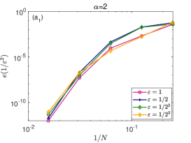
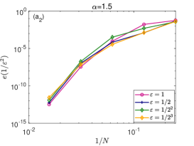
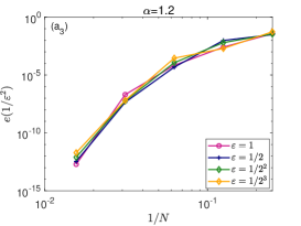
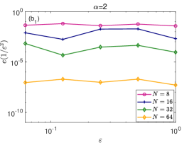
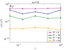
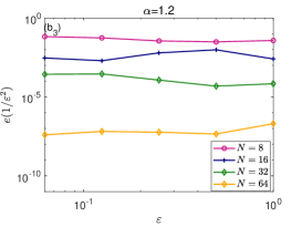
Figure 1: Long-time spatial errors for the NSFSGE in 2D at $t=1/\varepsilon^{2}$ with different $\alpha$.

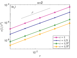
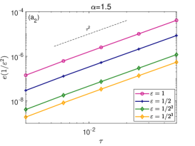
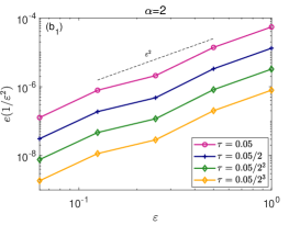
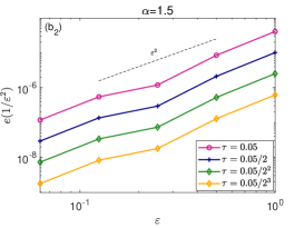
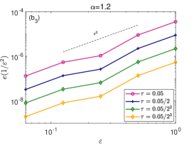
Figure 2: Long-time temporal errors for the NSFSGE in 2D at $t=1/\varepsilon^{2}$ with different $\alpha$.

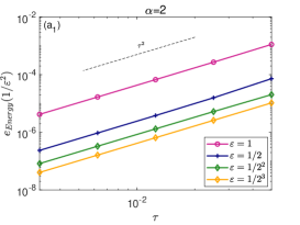
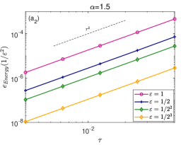
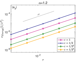
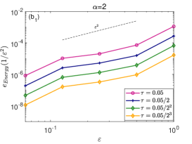
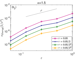
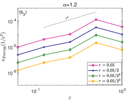
Figure 3: Long-time temporal errors for the discrete energy of the NSFSGE in 2D at $t=1/\varepsilon^{2}$ with different $\alpha$.

5.2 The long-time dynamics in 3D

We consider the NSFSGE (2) in 3D with the domain $(x,y,z)\in\Omega=(0,2)\times(0,2\pi)\times(0,2\pi)$ and the initial conditions are taken as

$$u_{0}(x,y,z)=\frac{1}{1+\sin^{2}(2\pi x+y+z)},\quad u_{1}(x,y,z)=\frac{2}{1+\sin^{2}(2\pi x+y+z)}.$$ (102)

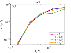
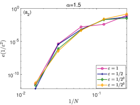
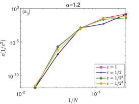
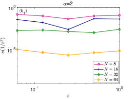
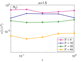
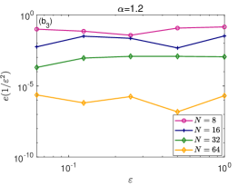
Figure 4: Long-time spatial errors for the NSFSGE in 3D at $t=1/\varepsilon^{2}$ with different $\alpha$.

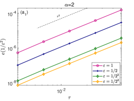
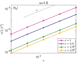
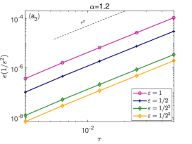
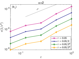
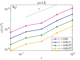
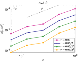
Figure 5: Long-time temporal errors for the NSFSGE in 3D at $t=1/\varepsilon^{2}$ with different $\alpha$.

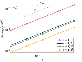
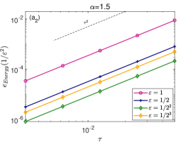
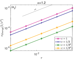
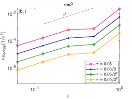
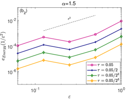
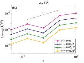
Figure 6: Long-time temporal errors of the discrete energy for the NSFSGE in 3D at $t=1/\varepsilon^{2}$ with different $\alpha$.

The numerical solutions with spatial nodes $N=128$ and time step $\tau=10^{-3}$ are used as the ‘exact’ solutions for comparison. Figure 4 shows the long-time spatial errors for different $N$ and $\varepsilon$ at $t=1/\varepsilon^{2}$ with $\alpha$ taken as 2, 1.5, 1.2. Similar to the 2D case, it is easy to see the spatial errors decay exponentially with $N$ for different fractional order $\alpha$ and vary little with the decreasing $\varepsilon$. Figure 5 shows the long-time temporal errors for different $\tau$ and $\varepsilon$ at $t=1/\varepsilon^{2}$ when $\alpha$ is taken as 2, 1.5, 1.2. From Figure 5, we can find that the temporal errors vary like $O(\varepsilon^{2}\tau^{2})$ up to the time at $O(1/\varepsilon^{2})$ and the fractional order $\alpha$ has no effect on the temporal errors, which shows the improved uniform error bound (72) holds in 3D. In addition, the improved uniform error bound $O(\varepsilon^{2}\tau^{2})$ of the discrete energy for the NSFSGE in 3D is further displayed in Figure 6.

5.3 The long-time dynamics for the oscillatory complex NSFSGE

We give some numerical results for the oscillatory complex NSFSGE (96) in 2D to demonstrate the improved error bound (98). We take $p=1$ and the initial values as

$$u_{0}(x,y)=x^{2}(x-1)^{2}+y(y-1)+6i,\quad u_{1}(x,y)=x(x-1)(2x-1)+y^{2}(y-1)^{2}+i\cos(2\pi x+2\pi y),\quad(x,y)\in\Omega=(0,1)^{2}.$$ (103)

The numerical solutions with spatial nodes $N=128$ and time step $\lambda=10^{-5}$ are chosen as the ‘exact’ solutions for comparison. The temporal errors are given for different fractional order $\alpha$ at $t=1$ in Tables 1-3. We can see the second-order convergence can be obtained for different $\alpha$ only when $\lambda\leq\varepsilon^{2}$, i.e., the upper triangle above the diagonal in Tables 1-3, which is in agreement with the theoretical analysis. This example indicates the TSFP method and the improved error bound (98) are effective for the oscillatory complex NSFSGE.

Table 1: Long-time temporal errors for the oscillatory complex NSFSGE in 2D when $\alpha=2$.

	$e(t=1)$		$\lambda_{0}=0.05$		$\lambda_{0}/4$		$\lambda_{0}/4^{2}$		$\lambda_{0}/4^{3}$		$\lambda_{0}/4^{4}$
	$\varepsilon=1$		4.5038e-01		2.5566e-02		1.5881e-03		9.9206e-05		6.1850e-06
	order		$-$		2.0694		2.0045		2.0003		2.0018
	$\varepsilon/2$		1.3076e-01		6.3988e-03		3.9449e-04		2.4628e-05		1.5354e-06
	order		$-$		2.1765		2.0099		2.0008		2.0018
	$\varepsilon/2^{2}$		7.8055e-01		3.9508e-02		2.4379e-03		1.5197e-04		9.4706e-06
	order		$-$		2.1521		2.0092		2.0019		2.0021
	$\varepsilon/2^{3}$		2.9970		9.7845e-02		4.7132e-03		3.0666e-04		1.7924e-05
	order		$-$		2.4684		2.1879		1.9710		2.0483
	$\varepsilon/2^{4}$		9.5838e-01		1.1325		4.0318e-02		2.2330e-03		1.4494e-04
	order		$-$		-0.1204		2.4060		2.0872		1.9728

Table 2: Long-time temporal errors for the oscillatory complex NSFSGE in 2D when $\alpha=1.5$.

	$e(t=1)$		$\lambda_{0}=0.05$		$\lambda_{0}/4$		$\lambda_{0}/4^{2}$		$\lambda_{0}/4^{3}$		$\lambda_{0}/4^{4}$
	$\varepsilon=1$		4.4357e-01		2.5201e-02		1.5669e-03		9.7883e-05		6.1025e-06
	order		$-$		2.0688		2.0038		2.0003		2.0018
	$\varepsilon/2$		1.2110e-01		6.3782e-03		3.9454e-04		2.4639e-05		1.5361e-06
	order		$-$		2.1234		2.0074		2.0006		2.0018
	$\varepsilon/2^{2}$		7.6497e-01		3.9335e-02		2.4323e-03		1.5189e-04		9.4695e-06
	order		$-$		2.1408		2.0077		2.0006		2.0018
	$\varepsilon/2^{3}$		3.0088		9.2594e-02		4.6984e-03		2.9035e-04		1.8089e-05
	order		$-$		2.5111		2.1503		2.0082		2.0023
	$\varepsilon/2^{4}$		9.6359e-01		1.1328		4.0355e-02		2.2183e-03		1.3740e-04
	order		$-$		-0.1167		2.4055		2.0926		2.0065

Table 3: Long-time temporal errors for the oscillatory complex NSFSGE in 2D when $\alpha=1.2$.

	$e(t=1)$		$\lambda_{0}=0.05$		$\lambda_{0}/4$		$\lambda_{0}/4^{2}$		$\lambda_{0}/4^{3}$		$\lambda_{0}/4^{4}$
	$\varepsilon=1$		4.4516e-01		2.5164e-02		1.5646e-03		9.7738e-05		6.0935e-06
	order		$-$		2.0724		2.0038		2.0003		2.0018
	$\varepsilon/2$		1.1653e-01		5.9772e-03		3.6915e-04		2.3051e-05		1.4371e-06
	order		$-$		2.1426		2.0086		2.0006		2.0018
	$\varepsilon/2^{2}$		1.6066		3.9512e-02		2.4438e-03		1.5261e-04		9.5146e-06
	order		$-$		2.6728		2.0076		2.0006		2.0018
	$\varepsilon/2^{3}$		2.9835		2.2866e-01		4.8089e-03		2.9648e-04		1.8469e-05
	order		$-$		1.8528		2.7857		2.0098		2.0024
	$\varepsilon/2^{4}$		9.7440e-01		1.1455		4.6627e-02		2.2205e-03		1.3759e-04
	order		$-$		-0.1167		2.3094		2.1961		2.0062

5.4 Applications

In this subsection, we give some applications to demonstrate the differences in the dynamic behaviors between the fractional sine-Gordon equation and the classical sine-Gordon equation. Numerical results of the NSFSGE with different initial conditions are obtained by the TSFP method.

5.4.1 Elliptical ring soliton in 2D

We consider the elliptical ring solitons with the initial conditions as [41]

$$u_{0}(x,y)=4\tan^{-1}\left(\exp\left(3-\sqrt{\frac{(x-y)^{2}}{3}+\frac{(x+y)^{2}}{2}}\right)\right),\quad u_{1}(x,y)=0,\quad-7\leq x,y\leq 7.$$ (104)

Here, we choose $N=256,\tau=10^{-3}$ to discrete the space and time domain, respectively. The numerical solutions of the NSFSGE in terms of $\sin(u/2)$ with different $\alpha$ at times $t=0,3,5,9,12,15$ are given in Figures 7-9. We can observe a clearly elliptical ring soliton at $t=0$. Then there is a small disturbance in the soliton and the soliton starts to shrink as the time changes, which can be seen at $t=3$ and $t=5$ clearly. From $t=9$, the soliton enters the expansion phase. This expansion is continued until $t=12$, where the soliton is nearly reformed. Finally, it seems to be in a shrinking phase again at $t=15$. Note that when $\alpha=2$, the nonlinear space fractional sine-Gordon equation reduces to the classical nonlinear sine-Gordon equation. The evolution trend of solitons in Figure 7 is consistent with the results in References [41, 42, 43, 44]. Furthermore, we can find the shape of the soliton changes with fractional order $\alpha$ varying, and the shape of the soliton changes more dramatically with $\alpha$ smaller.

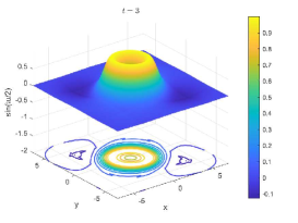
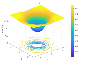
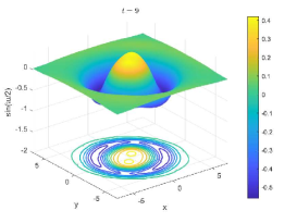
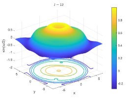
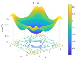
Figure 7: Surfaces and contour plots of the elliptical ring soliton when $\alpha=2$.

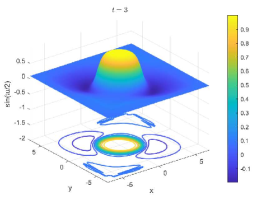
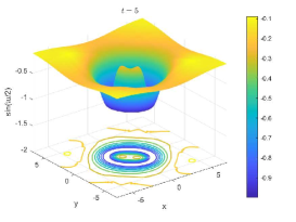
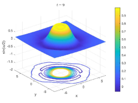
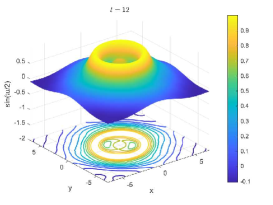
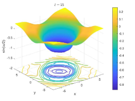
Figure 8: Surfaces and contour plots of the elliptical ring soliton in 2D when $\alpha=1.5$.

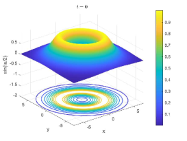
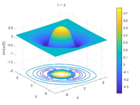
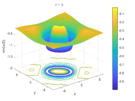
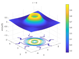
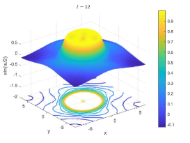
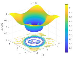
Figure 9: Surfaces and contour plots of elliptical ring soliton in 2D when $\alpha=1.2$.

5.4.2 Collisions of two circular solutions in 2D

We consider the circular ring solitons with the initial conditions as [45]

$$\begin{split}u_{0}(x,y)&=4\tan^{-1}\left[\exp\left(\frac{4-\sqrt{(x+3)^{2}+(y+7)^{2}}}{0.436}\right)\right],\quad-30\leq x\leq 10,\quad-21\leq y\leq 7,\\ u_{1}(x,y)&=4.13\operatorname{sech}\left(\frac{4-\sqrt{(x+3)^{2}+(y+7)^{2}}}{0.436}\right),\quad-30\leq x\leq 10,\quad-21\leq y\leq 7.\end{split}$$ (105)

We choose $N=256,\tau=10^{-3}$ to discrete the space and time domain. According to the symmetry properties of the problem, the solutions including the extension across $x=-10$ and $y=-7$ are provided. The surfaces and contour plots of two expanding circular ring solitons for different $\alpha$ at time $t=0,2,4,6,8,10$ are shown in Figures 10-12. From the contour plots, we can clearly observe the collision between two expanding circular ring solitons, where two smaller ring solitons emerge into a large ring soliton for different $\alpha$. Moreover, the smaller the fractional order $\alpha$, the stronger the shape change of the two solitons. The evolution trend of two circular ring solitons at $\alpha=2$ is consistent with the References [45, 46, 47, 48], which verifies the validity of our numerical method.

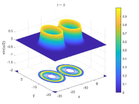
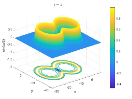
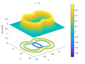
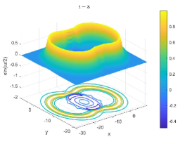
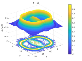
Figure 10: Surfaces and contour plots of the collisions of two circular ring soliton when $\alpha=2$.

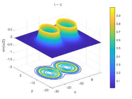
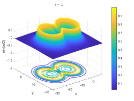
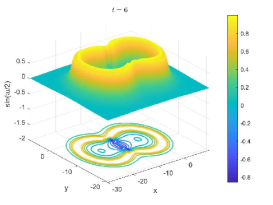
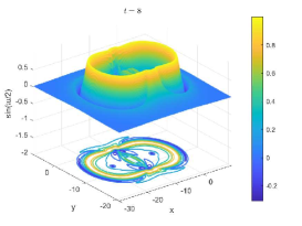
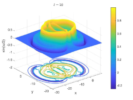
Figure 11: Surfaces and contour plots of the collisions of two circular ring soliton when $\alpha=1.5$.

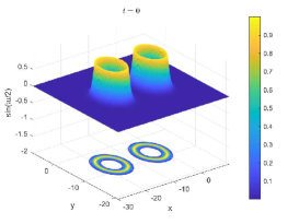
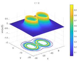
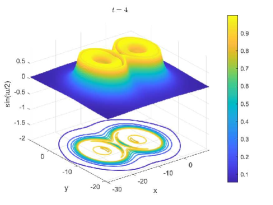
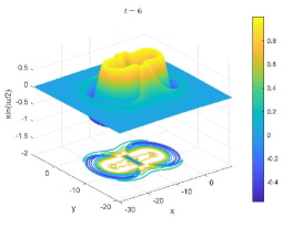
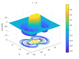
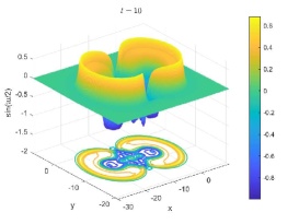
Figure 12: Surfaces and contour plots of the collisions of two circular ring soliton when $\alpha=1.2$.

5.4.3 Collisions of two circular solutions in 3D

We consider the circular solitons in 3D with the initial conditions as

$$\begin{split}u_{0}(x,y,z)&=4\tan^{-1}\left[\exp\left(\frac{4-\sqrt{(x+3)^{2}+(y+7)^{2}+(z+7)^{2}}}{0.436}\right)\right],\quad-30\leq x\leq 10,\quad-21\leq y,z\leq 7,\\ u_{1}(x,y,z)&=4.13\operatorname{sech}\left(\frac{4-\sqrt{(x+3)^{2}+(y+7)^{2}+(z+7)^{2}}}{0.436}\right),\quad-30\leq x\leq 10,\quad-21\leq y,z\leq 7.\end{split}$$ (106)

The step sizes $N=64,\tau=10^{-3}$ are taken to discrete the space and time domain. The extension over $x=-10$, $y=-7$ and $z=-7$ is included in the solution by the symmetry property of the problem. The isosurfaces of two expanding circular ring solitons in 3D for different $\alpha$ at time $t=0,2,3,4,5,6$ are exhibited in Figures 13-15. It is clearly shown the collision between two expanding circular ring solitons, where two smaller ring solitons emerge into a large ring soliton and then it again separates into two small circular solitons. We also can find the shapes of the two solitons change rapidly as the value of the fractional order $\alpha$ decreases. Thus the entire process for the collision between two expanding circular ring solitons is consistent with the 2D case.

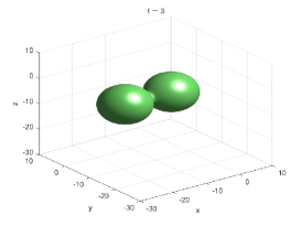
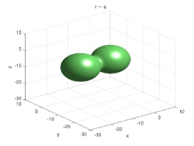
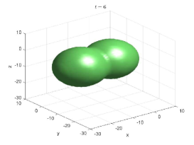
Figure 13: Isosurfaces for the collisions of two circular solitons in 3D when $\alpha=2$.

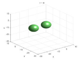
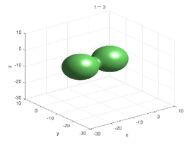
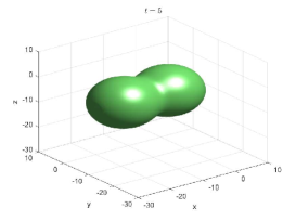
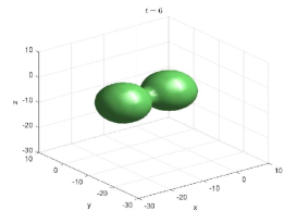
Figure 14: Isosurfaces for the collisions of two circular solitons in 3D when $\alpha=1.5$.

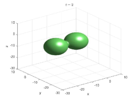
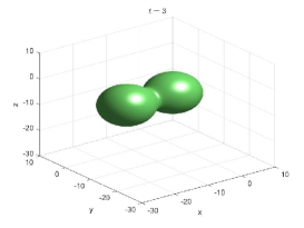
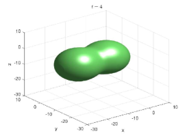
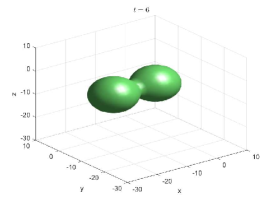
Figure 15: Isosurfaces for the collisions of two circular solitons in 3D when $\alpha=1.2$.

5.4.4 Collisions of four circular solutions in 3D

We consider the circular solitons in 3D with the initial conditions as

$$\begin{split}u_{0}(x,y,z)&=4\tan^{-1}\left[\exp\left(\frac{4-\sqrt{(x+3)^{2}+y^{2}+(z+3)^{2}}}{0.436}\right)\right],\quad-30\leq x,y,z\leq 10,\\ u_{1}(x,y,z)&=4.13\operatorname{sech}\left(\frac{4-\sqrt{(x+3)^{2}+y^{2}+(z+3)^{2}}}{0.436}\right),\quad-30\leq x,y,z\leq 10.\end{split}$$ (107)

We choose $N=64,\tau=10^{-3}$ to discrete the space and time domain. The extension over $x=-10$, $y=0$ and $z=-10$ is included in the solution based on the symmetry of the problem. The isosurfaces of four expanding circular ring solitons in 3D for different $\alpha$ at time $t=0,1,2,3,4,4.5$ are presented in Figures 16-18. We can see that these four circular solitons are initially independent of each other, gradually colliding and merging, and then separating into four new solitons. Moreover, as the fractional order $\alpha$ decreases, the shapes of circular solitons change more rapidly and the entire collision period becomes shorter.

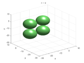
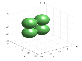
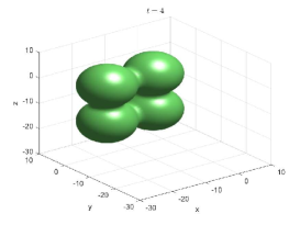
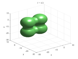
Figure 16: Isosurfaces for the collisions of four circular solitons in 3D when $\alpha=2$.

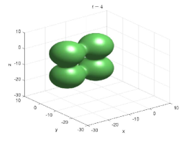
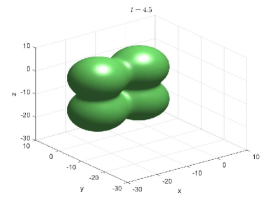
Figure 17: Isosurfaces for the collisions of four circular solitons in 3D when $\alpha=1.5$.

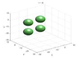
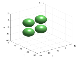
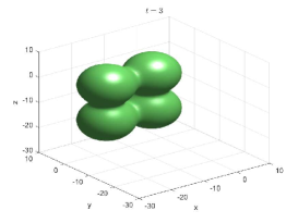
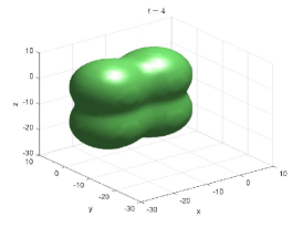
Figure 18: Isosurfaces for the collisions of four circular solitons in 3D when $\alpha=1.2$.

6 Conclusions

The improved uniform error bounds $O(h^{m}+\varepsilon^{2}\tau^{2})$ in $H^{\alpha/2}-$norm are established for the long-time dynamics of the high-dimensional NSFSGE. We first separate a linear part from the sine function of the NSFSGE and transform the NSFSGE to an equivalent NSFSE. Then the numerical scheme based on the time-splitting method in time and the Fourier pseudo-spectral method in space is developed, which can obtain the second-order convergence accuracy in time and the spectral convergence accuracy in space. By employing the RCO technique, the improved uniform error bounds $O(\varepsilon^{2}\tau^{2})$ for the semi-discrete scheme and $O(h^{m}+\varepsilon^{2}\tau^{2})$ for the full discrete scheme are obtained at time $T_{\varepsilon}$, which shows the explicit relationship between the error and $\varepsilon$. The error bounds $O(h^{m}+\varepsilon^{2}\tau^{2})$ for the discrete energy are also given. Further, the TSFP method and the improved error bounds are extended to the complex NSFSGE and the oscillatory complex NSFSGE. Finally, we give some numerical examples in 2D or 3D verifying that the error bounds in the theoretical analysis are sharp. We also give some applications to demonstrate the differences in the dynamic behaviors between the fractional sine-Gordon equation and classical sine-Gordon equation, which implies that the fractional order $\alpha$ has an obvious effect on dynamic behaviors of the NSFSGE. The numerical method and techniques used in this paper can be extended to the long-time dynamics research of other nonlinear fractional equations.

CRediT authorship contribution statement

Junqing Jia: Conceptualization, Methodology, Writing - original draft, Software. Xiaoqing Chi: Conceptualization, Methodology, Writing - review & editing, Software. Xiaoyun Jiang: Conceptualization, Methodology, Writing - review & editing, Supervision.

Declaration of competing interest

The authors declare that they have no known competing financial interests or personal relationships that could have appeared to influence the work reported in this paper.

Data Availability

The datasets analysed during the current study are available from the corresponding author on reasonable request.

References

- [1] S. Britt, E. Turkel, S. Tsynkov, High order compact time/space finite difference scheme for the wave equation with variable speed of sound, J. Sci. Comput. 76 (2018) 777-811.
- [2] K. Geng, B. Zhu, Q. Cao, C. Dai, Y. Wang, Nondegenerate soliton dynamics of nonlocal nonlinear Schrödinger equation, Nonlinear Dynam. 111 (2023) 16483-16496.
- [3] B. Hou, D. Liang, Energy-preserving time high-order AVF compact finite difference schemes for nonlinear wave equations with variable coefficients, J. Comput. Phys. 421 (2020) 109738.
- [4] W. Strauss, Nonlinear wave equations, American Mathematical Society, 1990.
- [5] P. Sheng, Chaos and turbulence in the generalized Sine-Gordon equation, J. Appl. Math. 28 (2005) 453-457.
- [6] C. Jesús, P. Kevrekidis, F. Williams, The sine-Gordon model and its applications, Springer, 2014.
- [7] A. Mohebbi, M. Dehghan, High-order solution of one-dimensional sine-Gordon equation using compact finite difference and DIRKN methods, Math. Comput. Model 51 (2010) 537-549.
- [8] A. Wazwaz, The tanh method: exact solutions of the sine-Gordon and the sinh-Gordon equations, Appl. Math. Comput. 167 (2005) 1196-1210.
- [9] S. Silling, E. Madenci, Editorial: The world is nonlocal. J. Peridyn. Nonlocal Model. 1 (2019), 1-2.
- [10] F. Zeng, F. Liu, C. Li, K. Burrage, I. Turner, V. Anh, A Crank-Nicolson ADI spectral method for a two-dimensional Riesz space fractional nonlinear reaction-diffusion equation, SIAM J. Numer. Anal. 52 (2014) 2599-2622.
- [11] M. Amabili, P. Balasubramanian, G. Ferrari, Nonlinear vibrations and damping of fractional viscoelastic rectangular plates, Nonlinear Dyn. 4 (2020) 1-29.
- [12] J. Jia, X. Zheng, H. Wang, Numerical discretization and fast approximation of a variably distributed-order fractional wave equation, ESAIM-Math. Model. Num. 55 (2021) 2211-2232.
- [13] F. Liu, P. Zhuang, Q. Liu, Numerical methods of fractional partial differential equations and their applications, Science Press, 2015.
- [14] V. Tarasov, E. Aifantis, Non-standard extensions of gradient elasticity: fractional non-locality, memory and fractality, Commun. Nonlinear Sci. 22 (2015) 197-227.
- [15] Y. Fu, W. Cai, Y. Wang, A linearly implicit structure-preserving scheme for the fractional sine-Gordon equation based on the IEQ approach, Appl. Numer. Math. 160 (2021) 368-385.
- [16] N. Korabel, G. Zaslavsky, V. Tarasov, Coupled oscillators with power-law interaction and their fractional dynamics analogues, Commun. Nonlinear Sci. 12 (2007) 1405-1417.
- [17] J. Macías-Díaz, Numerical study of the process of nonlinear supratransmission in Riesz space-fractional sine-Gordon equations, Commun. Nonlinear Sci. 46 (2017) 89-102.
- [18] Y. Huang, A. Oberman, Numerical methods for the fractional Laplacian: a finite difference-quadrature approach, SIAM J. Numer. Anal. 52 (2014) 3056-3084.
- [19] A. Lischke, G. Pang, M. Gulian, et al. What is the fractional Laplacian? A comparative review with new results, J. Comput. Phys. 404 (2020) 109009.
- [20] M. Ainsworth, Z. Mao, Analysis and approximation of a fractional Cahn-Hilliard equation, SIAM J. Numer. Anal. 55 (2017) 1689-1718.
- [21] D. Hu, W. Cai, Z. Xu, Y. Bo, Y. Wang, Dissipation-preserving Fourier pseudo-spectral method for the space fractional nonlinear sine-Gordon equation with damping, Math. Comput. Simulat. 188 (2021) 35-59.
- [22] J. Delort, J. Szeftel, Long-time existence for small data nonlinear Klein-Gordon equations on tori and spheres, Int. Math. Res. Notices 37 (2004) 1897-1966.
- [23] D. Fang, Q. Zhang, Long-time existence for semi-linear Klein-Gordon equations on tori, J. Differ. Equations 249 (2010) 151-179.
- [24] O. Nikan, Z. Avazzadeh, J. Machado, Numerical investigation of fractional nonlinear sine-Gordon and Klein-Gordon models arising in relativistic quantum mechanics, Eng. Anal. Bound. Elem. 120 (2020) 223-237.
- [25] M. Ran, C. Zhang, Compact difference scheme for a class of fractional-in-space nonlinear damped wave equations in two space dimensions, Comput. Math. Appl. 71 (2016) 1151-1162.
- [26] G. Alfimov, T. Pierantozzi, L. Vázquez, Numerical study of a fractional sine-Gordon equation, Fractional Differ. Appl. 4 (2004) 153-162.
- [27] Y. Cai, Y. Wang, A uniformly accurate (UA) multiscale time integrator pseudospectral method for the nonlinear Dirac equation in the nonrelativistic limit regime, ESAIM-Math. Model. Num. 52 (2018) 543-566.
- [28] W. Bao, Y. Cai, Y. Feng, Improved uniform error bounds of the time-splitting methods for the long-time (nonlinear) Schrödinger equation, Math. Comput. 92 (2023) 1109-1139.
- [29] W. Bao, Y. Cai, Y. Feng, Improved uniform error bounds on time-splitting methods for long-time dynamics of the nonlinear Klein-Gordon equation with weak nonlinearity, SIAM J Numer Anal. 60 (2022) 1962-1984.
- [30] D. Cohen, H. Ernst, C. Lubich, Long-time analysis of nonlinearly perturbed wave equations via modulated Fourier expansions, Arch. Ration. Mech. An. 187 (2008) 341-368.
- [31] Y. Feng, Long time error analysis of the fourth-order compact finite difference methods for the nonlinear Klein-Gordon equation with weak nonlinearity, Numer. Meth. Part. D. E. 37 (2021) 897-914.
- [32] Y. Feng, W. Yi, Uniform Error Bounds of an Exponential Wave Integrator for the long-time Dynamics of the Nonlinear Klein-Gordon Equation, Multiscale. Model. Sim. 19 (2021) 1212-1235.
- [33] S. Duo, Y. Zhang, Mass-conservative Fourier spectral methods for solving the fractional nonlinear Schrödinger equation, Comput. Math. Appl. 71 (2016) 2257-2271.
- [34] S. Zhai, D. Wang, Z. Weng, X. Zhao, Error analysis and numerical simulations of Strang splitting method for space fractional nonlinear Schrödinger equation, J. Sci. Comput. 81 (2019) 965-989.
- [35] C. Lubich, On splitting methods for Schrödinger-Poisson and cubic nonlinear Schrödinger equations, Math. Comput. 77 (2008) 2141-2153.
- [36] C. Su, X. Zhao, On time-splitting methods for nonlinear Schrödinger equation with highly oscillatory potential, ESAIM-Math. Model. Num. 54 (2020) 1491-1508.
- [37] J. Jia, X. Jiang, Improved uniform error bounds of exponential wave integrator method for long-time dynamics of the space fractional Klein-Gordon equation with weak nonlinearity, J. Sci. Comput. https://doi.org/10.1007/s10915-023-02376-2.
- [38] J. Shen, T. Tang, L. Wang. Spectral Methods. Springer, 2011.
- [39] A. Quarteroni, A. Valli, Numerical Approximation of Partial Differential Equations, Springer, 1994.
- [40] H. Zhang, X. Jiang, F. Zeng, G. Karniadakis, A stabilized semi-implicit Fourier spectral method for nonlinear space-fractional reaction-diffusion equations, J. Comput. Phys. 405 (2019) 109141.
- [41] M. Dehghan, A. Ghesmati, Numerical simulation of two-dimensional sine-Gordon solitons via a local weak meshless technique based on the radial point interpolation method (RPIM), Comput. Phys. Comm. 181 (2010) 772-786.
- [42] R. Jiwari, S. Pandit, R. Mittal, Numerical simulation of two-dimensional sine-Gordon solitons by differential quadrature method, Comput. Phys. Comm. 183 (2012) 600-616.
- [43] R. Jiwari, Barycentric rational interpolation and local radial basis functions based numerical algorithms for multidimensional sine-Gordon equation, Numer. Meth. Part. D. E. 37 (2021) 1965-1992.
- [44] C. Wang, Convergence of the interpolated coefficient finite element method for the two-dimensional elliptic sine-Gordon equations, Numer. Meth. Part. D. E. 27 (2011) 387-398.
- [45] W. Cai, C. Jiang, Y. Wang, Y. Song, Structure-preserving algorithms for the two-dimensional sine-Gordon equation with Neumann boundary conditions, J. Comput. Phys. 395 (2019) 166-185.
- [46] K. Djidjeli, W. Price, E. Twizell, Numerical solutions of a damped sine-Gordon equation in two space variables, J. Eng. Math. 29 (1995) 347-369.
- [47] A. Khaliq, B. Abukhodair, Q. Sheng, A predictor-corrector scheme for the sine-Gordon equation, Numer. Meth. Part. D. E. 16 (2000) 133-146.
- [48] C. Jiang, W. Cai, Y. Wang, A linearly implicit and local energy-preserving scheme for the sine-Gordon equation based on the invariant energy quadratization approach, J. Sci. Comput. 88 (2019) 1629-1655.