Six-Point Method for Multi-Camera Systems with Reduced Solution Space

Abstract

Relative pose estimation using point correspondences (PC) is a widely used technique. A minimal configuration of six PCs is required for generalized cameras. In this paper, we present several minimal solvers that use six PCs to compute the 6DOF relative pose of a multi-camera system, including a minimal solver for the generalized camera and two minimal solvers for the practical configuration of two-camera rigs. The equation construction is based on the decoupling of rotation and translation. Rotation is represented by Cayley or quaternion parametrization, and translation can be eliminated by using the hidden variable technique. Ray bundle constraints are found and proven when a subset of PCs relate the same cameras across two views. This is the key to reducing the number of solutions and generating numerically stable solvers. Moreover, all configurations of six-point problems for multi-camera systems are enumerated. Extensive experiments demonstrate that our solvers are more accurate than the state-of-the-art six-point methods, while achieving better performance in efficiency.

1 Introduction

Relative pose estimation utilizing feature correspondences is a fundamental problem in geometric computer vision. It plays a crucial role in numerous tasks such as autonomous driving, augmented reality, simultaneous localization and mapping, etc. Despite having a long history, the research on relative pose estimation remains active. These efforts focus on enhancing the efficiency, stability, and accuracy of algorithms [14, 2, 7, 13, 16].

Camera models have a significant impact on computing the relative pose. A pinhole or perspective camera model is used to model a single camera [19], and more complicated cameras like multi-camera systems require a generalized camera model for modeling [12, 42, 48]. A generalized camera can be formed by abstracting the landmark observations into spatial rays, which do not necessarily require originating from the projection center. This paper is principally concerned with a multi-camera setup comprising several cameras that have been installed rigidly. As we shall demonstrate in this paper, $n$ point correspondences (PCs) for a generalized camera can be represented similarly by using $2n$ single cameras in a multi-camera system. It is a common belief that the standard epipolar geometry using five PCs is incapable of recovering the scale of translation [19]. Conversely, the translation scale of multi-camera systems can be uniquely determined, and the minimum requirement for solving the relative pose increases from five to six PCs across both views [46].

Due to the presence of outliers in PCs, a robust estimator is essential for accurate relative pose estimation and outlier rejection. The random sample consensus (RANSAC) framework [9] and its various adaptations [30, 44, 1, 3] are widely employed in computer vision community. A minimal solver is the core component in the RANSAC framework. Based on the epipolar geometry of each PC, one constraint for solving relative pose can be established [19]. Various methods for computing relative pose of a single camera are known as five-point methods [40, 47, 34, 26, 27, 8]. The six-point method [46] is the first minimal solver proposed for computing relative pose of a multi-camera system. Numerous methods have been introduced subsequently, such as the enhanced version of the six-point method [5], the seventeen-point linear solvers [35, 22], an iterative optimization-based solver [24], and a global optimization-based solver [53].

This paper estimates the full DOF relative pose for a multi-camera system using PCs. The main contributions of this work are as follows:

• We estimate 6DOF relative pose from a minimal number of six PCs for multi-camera systems. A generic minimal solver for the generalized camera and two minimal solvers for popular configurations of two-camera rigs are proposed. Moreover, we enumerate all configurations of minimal six-point problems for multi-camera systems.

• For multi-camera systems, when a subset of PCs relate the same cameras across two views, ray bundle constraints are found and proven. It can be seen that using ray bundle constraints reduces the number of solutions and generates numerically stable solvers for relative pose estimation.

• We exploit a framework by decoupling rotation and translation. Rotation can be represented by Cayley or quaternion parametrization, and translation is eliminated by using the hidden variable technique. This framework can easily deal with relative pose estimation for other configurations of multi-camera systems.

2 Related Work

The research on relative pose estimation remains active in geometric vision, with a lot of classical solvers existing in this area. First, these solvers can be divided into the relative pose estimation for single cameras [19, 40, 47, 34, 26, 27, 8], multi-camera systems or generalized cameras [46, 35, 22, 24, 53]. These cameras can be calibrated or partially uncalibrated with unknown focal length or radial distortion.

Second, the relative pose estimation solvers can be categorized as minimal solvers [40, 46], non-minimal solvers [22, 25, 24, 53, 51] and linear solvers [20, 35]. The minimal solvers aim to estimate relative pose using the minimum number of geometric primitives. The non-minimal solvers leverage all the feature correspondences to compute the relative pose. The linear solvers require more feature correspondences than the minimal solvers, and their primary purpose is to provide a straightforward and efficient solution. To achieve computational efficiency, the linear solvers often ignore implicit constraints on unknown parameters. Conversely, the minimal and non-minimal solvers usually exploit implicit constraints while solving for unknowns. When dealing with feature correspondences that may contain outliers, minimal solvers play a crucial role in ensuring robust estimation. For instance, RANSAC and its variants depend heavily on efficient minimal solvers.

The combination of the two aspects mentioned above produces many subcategories. In this paper, we focus on exploring the minimal solvers for multi-camera systems using PCs. A minimal solver was first proposed to solve the relative pose of multi-camera systems using $6$ PCs [46]. Then, a linear solver taking $17$ PCs was introduced in [35, 22]. Several solvers were developed for applying to structure-from-motion with special configurations [54, 21]. Several non-minimal solvers were proposed which leverage either local optimization [24] or global optimization [53] to determine optimal relative poses. Some solvers required the motion priors of multi-camera systems, including known rotation axis [32, 49, 37] and Ackermann motion [31]. Moreover, an efficient solver was achieved by implementing a first-order approximation of relative pose  [50].

3 Relative Pose Estimation for Generalized Cameras

This section presents a novel six-point method for multi-camera systems and generalized cameras by decoupling rotation and translation. The ray bundle constraints are proven and exploited for solution space reduction. In addition, all configurations of minimal six-point problems for multi-camera systems are enumerated in this paper.

3.1 Geometric Constraints

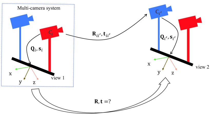
Figure 1: Relative pose estimation for a multi-camera system. A point is captured by perspective camera $C_{i}$ in view 1 and camera $C_{i^{\prime}}$ in view 2. $\{\mathbf{Q}_{i},\mathbf{s}_{i}\}$ and $\{\mathbf{Q}_{i^{\prime}},\mathbf{s}_{i^{\prime}}\}$ are extrinsic parameters for $C_{i}$ and $C_{i^{\prime}}$, respectively. The related point correspondence can be described by the two-view geometry of cameras $C_{i}$ and $C_{i^{\prime}}$.

Fig. 1 illustrates a multi-camera system consisting of multiple perspective cameras, assuming that the intrinsic and extrinsic parameters of perspective cameras have been calibrated. The extrinsic parameters of the $i$-th camera are denoted as $\{\mathbf{Q}_{i},\mathbf{s}_{i}\}$, which are the relative rotation and translation to the reference of the multi-camera system. Let $\mathbf{R}$ and $\mathbf{t}$ denote the relative rotation and translation between the first and second views, respectively.

A PC in a multi-camera system establishes the relationship of a point captured by two perspective cameras across two different views. Let the $k$-th PC be denoted by $(\mathbf{x}_{k},\mathbf{x}^{\prime}_{k},i_{k},i^{\prime}_{k})$. This indicates that the $i_{k}$-th camera captures a point in the first view, which is represented by its homogeneous coordinate in the normalized image plane denoted as $\mathbf{x}_{k}$. Furthermore, this same point is also captured by the $i^{\prime}_{k}$-th camera in the second view, which is represented by its homogeneous coordinate as $\mathbf{x}^{\prime}_{k}$. In the following text, we omit the subscript $k$ of camera indices $i$ and $i^{\prime}$ to simplify the notation. In a multi-camera system, the essential matrices for different PCs are typically distinct, which sets it apart from the case of two-view geometry for a single camera. Thus, one constraint of epipolar geometry [19] introduced by the $k$-th PC is

$$\mathbf{x}_{k}^{\prime T}\mathbf{E}_{k}\mathbf{x}_{k}=0,$$ (1)

where the essential matrix is represented as

$$\mathbf{E}_{k}=[\mathbf{t}_{ii^{\prime}}]_{\times}\mathbf{R}_{ii^{\prime}}.$$ (2)

Here $\{\mathbf{R}_{ii^{\prime}},\mathbf{t}_{ii^{\prime}}\}$ is the relative rotation and translation from camera $i$ in the first view to camera $i^{\prime}$ in the second view. According to Fig. 1, it is obtained by a composition of three spatial transformations as

$$\begin{bmatrix}\mathbf{R}_{ii^{\prime}}&{\mathbf{t}_{ii^{\prime}}}\\ {{\mathbf{0}}}&{1}\\ \end{bmatrix}= \begin{bmatrix}{\mathbf{Q}_{i^{\prime}}}&{\mathbf{s}_{i^{\prime}}}\\ {{\mathbf{0}}}&{1}\\ \end{bmatrix}^{-1}\begin{bmatrix}\mathbf{R}&{\mathbf{t}}\\ {{\mathbf{0}}}&{1}\\ \end{bmatrix}\begin{bmatrix}{\mathbf{Q}_{i}}&{\mathbf{s}_{i}}\\ {{\mathbf{0}}}&{1}\\ \end{bmatrix}$$

$$= \begin{bmatrix}{\mathbf{Q}_{i^{\prime}}^{T}\mathbf{R}\mathbf{Q}_{i}}&\mathbf{Q}_{i^{\prime}}^{T}(\mathbf{R}\mathbf{s}_{i}+\mathbf{t}-\mathbf{s}_{i^{\prime}})\\ {{\mathbf{0}}}&\ {1}\\ \end{bmatrix}.$$ (3)

By substituting $\mathbf{R}_{ii^{\prime}}$ and $\mathbf{t}_{ii^{\prime}}$ into Eq. (2), the essential matrix $\mathbf{E}_{k}$ can be reformulated as

$$\mathbf{E}_{k}=\mathbf{Q}_{i^{\prime}}^{T}(\mathbf{R}[\mathbf{s}_{i}]_{\times}+[\mathbf{t}-\mathbf{s}_{i^{\prime}}]_{\times}\mathbf{R})\mathbf{Q}_{i}.$$ (4)

Based on the above equation, it can be seen that Eq. (1) is bilinear in the relative pose $(\mathbf{R},\mathbf{t})$.

3.2 Relative Pose Parameterization

We need to parametrize the relative pose of multi-camera systems. Rotation can be parameterized by Cayley parametrization, quaternions, Euler angles, direction cosine matrix (DCM), etc. Cayley and quaternion parameterizations have shown superiority in minimal problems [52]. Rotation $\mathbf{R}$ using Cayley parameterization can be written as

$$\mathbf{R}_{\text{cayl}}=\small{\frac{1}{q_{x}^{2}+q_{y}^{2}+q_{z}^{2}+1}}\ .$$

$$\small{\begin{bmatrix}{1+q_{x}^{2}-q_{y}^{2}-q_{z}^{2}}&2q_{x}q_{y}-2q_{z}&2q_{x}q_{z}+2q_{y}\\ 2q_{x}q_{y}+2q_{z}&1-q_{x}^{2}+q_{y}^{2}-q_{z}^{2}&2q_{y}q_{z}-2q_{x}\\ 2q_{x}q_{z}-2q_{y}&2q_{y}q_{z}+2q_{x}&{1-q_{x}^{2}-q_{y}^{2}+q_{z}^{2}}\end{bmatrix}},$$ (5)

where $[1,q_{x},q_{y},q_{z}]^{T}$ is a homogeneous quaternion vector. Rotation matrix $\mathbf{R}$ using quaternion parameterization can be written as

$$\mathbf{R}_{\text{quat}}=$$

$$\small{\begin{bmatrix}q_{w}^{2}+q_{x}^{2}-q_{y}^{2}-q_{z}^{2}&2q_{x}q_{y}-2q_{w}q_{z}&2q_{x}q_{z}+2q_{w}q_{y}\\ 2q_{x}q_{y}+2q_{w}q_{z}&q_{w}^{2}-q_{x}^{2}+q_{y}^{2}-q_{z}^{2}&2q_{y}q_{z}-2q_{w}q_{x}\\ 2q_{x}q_{z}-2q_{w}q_{y}&2q_{y}q_{z}+2q_{w}q_{x}&q_{w}^{2}-q_{x}^{2}-q_{y}^{2}+q_{z}^{2}\end{bmatrix}},$$ (6)

where $[q_{w},q_{x},q_{y},q_{z}]^{T}$ is a normalized quaternion vector satisfying the following constraints:

$$q_{w}^{2}+q_{x}^{2}+q_{y}^{2}+q_{z}^{2}=1.$$ (7)

Note that $180^{\circ}$ rotations are prohibited in Cayley parameterization, but this is a rare case for usual image pairs. In practice, it has been widely used in minimal problems [45, 24, 54, 52]. By contrast, quaternion parameterization does not have any degeneracy. However, quaternion introduces more variables than Cayley, so its solvers are usually less efficient. We construct solvers using both of these two parameterizations for completeness. In the following, we introduce the solver generation procedure based on Cayley parameterization. This procedure can also be applied to quaternion parameterization straightforwardly.

The translation $\mathbf{t}$ can be parametrized as

$$\mathbf{t}=\begin{bmatrix}{t_{x}}&\ {t_{y}}&\ {t_{z}}\end{bmatrix}^{T}.$$ (8)

3.3 Equation System Construction

For multi-camera systems, the relative pose between two views is 6DOF. Thus, the relative pose estimation of a multi-camera system requires a minimal number of six PCs. Using Cayley parameterization, we obtain six polynomials for six unknowns $\{q_{x},q_{y},q_{z},t_{x},t_{y},t_{z}\}$ from Eq. (1) by substituting the essential matrix (4) into them. After separating $q_{x}$, $q_{y}$, $q_{z}$ from $t_{x}$, $t_{y}$, $t_{z}$, we arrive at an equation system

$$\underbrace{{\mathbf{M}}(q_{x},q_{y},q_{z})}_{6\times 4}\begin{bmatrix}{{{t}_{x}}}\\ {{{t}_{y}}}\\ {{{t}_{z}}}\\ 1\end{bmatrix}={\mathbf{0}},$$ (9)

where the entries of ${\mathbf{M}}$ are quadratic polynomials with three unknowns $q_{x},q_{y},q_{z}$. The $i$-th row corresponds to the constraint of $i$-th PC. It can be seen that ${\mathbf{M}}$ has a null vector. Thus, the determinants of all the $4\times 4$ submatrices of ${\mathbf{M}}$ should be zero.

Moreover, when a subset of PCs relates the same perspective cameras across two views, there is a property for this scenario. This scenario can be used to reduce the number of solutions and generate numerically stable solvers.

Theorem 1.

Denote $\mathcal{S}$ as a matrix set with elements satisfying $\mathbf{N}={\mathbf{M}}([k_{1},k_{2},k_{3}],1:3)$, where $\mathbf{N}$ is formed from rows $\{k_{1},k_{2},k_{3}\}$ and columns $\{1,2,3\}$ of $\mathbf{M}$. In addition, $k_{1}$-th, $k_{2}$-th, and $k_{3}$-th PCs are captured by the same perspective cameras across two views and $k_{1}<k_{2}<k_{3}$. Then $\operatorname*{rank}(\mathbf{N})=2$, $\forall\mathbf{N}\in\mathcal{S}$ holds for non-degenerate cases.

Proof.

Let us investigate an arbitrary element of $\mathcal{S}$. Denote it is the $k$-th element $\mathbf{N}_{k}$ in $\mathcal{S}$. The extrinsic parameters of the related perspective camera in view 1 is $\{\mathbf{Q}_{i},\mathbf{s}_{i}\}$, and the extrinsic parameters of the related perspective camera in view 2 is $\{\mathbf{Q}_{i^{\prime}},\mathbf{s}_{i^{\prime}}\}$.

First we prove that $\operatorname*{rank}(\mathbf{N}_{k})\leq 2$. To achieve this goal, we need to prove that the null space of $\mathbf{N}_{k}$ is not empty. Since $k_{1}$-th, $k_{2}$-th, and $k_{3}$-th PCs are captured by the same perspective cameras across two views, their related essential matrices are the same. According to Eq. (4), the essential matrix is

$$\mathbf{E}_{k}=\mathbf{Q}_{i^{\prime}}^{T}[\mathbf{t}+\mathbf{R}\mathbf{s}_{i}-\mathbf{s}_{i^{\prime}}]_{\times}\mathbf{R}\mathbf{Q}_{i}.$$ (10)

Denote $\bar{\mathbf{t}}\triangleq\mathbf{t}+\mathbf{R}\mathbf{s}_{i}-\mathbf{s}_{i^{\prime}}$, then we have

$$\mathbf{E}_{k}=\mathbf{Q}_{i^{\prime}}^{T}[\bar{\mathbf{t}}]_{\times}\mathbf{R}\mathbf{Q}_{i}.$$ (11)

Substituting Eq. (11) into Eq. (1), we obtain three equations for the three PCs. Each monomial in the three equations is linear with respect to one entry of vector $\bar{\mathbf{t}}$, and there is no constant term. Hence, these equations can be expressed as

$$\frac{1}{q_{x}^{2}+q_{y}^{2}+q_{z}^{2}+1}\mathbf{A}_{k}\bar{\mathbf{t}}=\mathbf{0},$$ (12)

$$\Rightarrow \mathbf{A}_{k}(\mathbf{t}+\mathbf{R}\mathbf{s}_{i}-\mathbf{s}_{i^{\prime}})=\mathbf{0},$$ (13)

$$\Rightarrow \begin{bmatrix}\mathbf{A}_{k}&\mathbf{A}_{k}(\mathbf{R}\mathbf{s}_{i}-\mathbf{s}_{i^{\prime}})\end{bmatrix}\begin{bmatrix}\mathbf{t}\\ 1\end{bmatrix}=\mathbf{0}.$$ (14)

By comparing the construction procedure of Eq. (9) and Eq. (14), we can see that

$$\mathbf{A}_{k}={\mathbf{M}}([k_{1},k_{2},k_{3}],1:3)=\mathbf{N}_{k}.$$ (15)

Substituting this equation into Eq. (12), we can see that the null space of $\mathbf{N}_{k}$ is not empty.

Next we prove that $\operatorname*{rank}(\mathbf{N}_{k})\geq 2$. We achieve this goal using proof by contradiction. If $\operatorname*{rank}(\mathbf{N}_{k})\leq 1$, then $\operatorname*{rank}({\mathbf{M}}([k_{1},k_{2},k_{3}],{1:4}))\leq 2$ considering that ${\mathbf{M}}([k_{1},k_{2},k_{3}],1:4)$ has one more column than $\mathbf{N}_{k}$. This means the three PCs provide at most two independent constraints for the relative pose estimation. This does not hold true for non-degenerate cases, hence invalidating the assumption that $\operatorname*{rank}(\mathbf{N}_{k})\leq 1$. It can be seen that the rank of $\mathbf{N}$ is 2 in non-degenerate cases. ∎

We call the constraints in Theorem 1 as the ray bundle constraints. In computer graphics, a ray bundle is a collection of light rays that share a common origin and propagate in different directions. In addition, a factor $q_{x}^{2}+q_{y}^{2}+q_{z}^{2}+1$ can be factored out to simplify the equation system. Please see the supplementary material for proof. It will generate more efficient solvers and sometimes avoid extraneous roots. In summary, the whole polynomial equation system consists of two types of constraints, which can be written as

$${\mathcal{E}}_{1}\triangleq\{\operatorname*{quot}(\det(\mathbf{N}),q_{x}^{2}+q_{y}^{2}+q_{z}^{2}+1)=0\ |$$

$$\mathbf{N}\in 4\times 4\text{ submatrices of }{\mathbf{M}}\},$$ (16)

and

$${\mathcal{E}}_{2}\triangleq\{\operatorname*{quot}(\det(\mathbf{N}),q_{x}^{2}+q_{y}^{2}+q_{z}^{2}+1)=0\ |\mathbf{N}\in\mathcal{S}\},$$ (17)

where $\operatorname*{quot}(a,b)$ means quotient of $a$ divided by $b$, and $\det(\cdot)$ means the determinant operator.

There are $15$ equations of degree $6$ and some equations of degree 4 in ${\mathcal{E}}_{1}$ and ${\mathcal{E}}_{2}$, respectively. Note that the number of equations in ${\mathcal{E}}_{2}$ varies for different PC configurations. ${\mathcal{E}}_{2}$ can be an empty set for certain PC configurations of multi-camera systems.

Once the rotation parameters $\{q_{x},q_{y},q_{z}\}$ have been obtained, the translation $[t_{x},t_{y},t_{z}]^{T}$ can be recovered by first calculating a vector in the null space of $\mathbf{M}$, and then normalizing the vector by dividing its last entry.

3.4 Polynomial System Solving

Based on the polynomial equation system Eqs. (16) and (17), we propose a minimal generic solver for the generalized camera and two minimal solvers for standard configurations of two-camera rigs. The Gröbner basis technique can be used to find algebraic solutions to the polynomial equation system [28, 39]. Firstly, we construct a random instance of the original equation system in a finite prime field $\mathbb{Z}_{p}$ [36] or a rational field. This is beneficial for maintaining numerical stability and eliminating large number arithmetic during the calculation of Gröbner basis. Secondly, Macaulay 2 [11] is used to calculate Gröbner basis. Finally, we use an automatic Gröbner basis solver [28] to find the solver of the polynomial equation system. It should be noted that the polynomial equations $\mathcal{E}_{1}$ and $\mathcal{E}_{2}$ can be extended to deal with relative pose estimation for other configurations of multi-camera systems, such as with partially uncalibrated cameras and known rotation angles.

3.4.1 Minimal Solver for Generalized Cameras

We propose a generic solver for the generalized camera given six PCs. As shown in Fig. 2, there are two views of a generalized camera, and there are 6 PCs across two views. We can define 12 virtual perspective cameras by the following method. The origins $o_{1},\cdots,o_{6}$ and $o^{\prime}_{1},\cdots,o^{\prime}_{6}$ of the virtual cameras are the positions of PCs. The orientations of these virtual cameras are consistent with the generalized camera’s reference. The 6 PCs can be equivalently captured by a virtual 12-camera rig. Moreover, we can calculate the extrinsic parameters of these 12 virtual perspective cameras and the image coordinates of PCs in these virtual cameras. As a result, we can construct a minimal generic solver to recover the relative pose of the generalized camera.

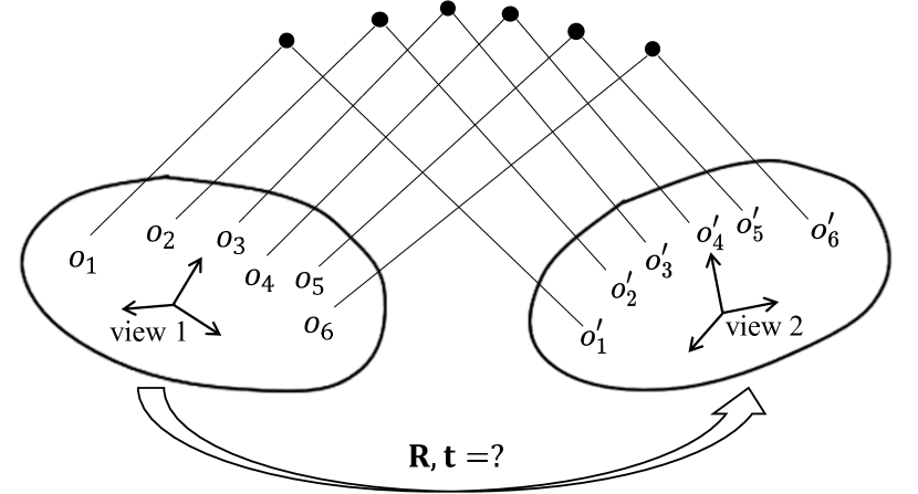
Figure 2: Relative pose estimation for generalized cameras. Specifically, two-view geometry for 6 PCs and a generalized camera can be described by a 12-camera rig. Note that points $o_{i}$ and $o^{\prime}_{i}$ do not necessarily correspond to the same physical point of the generalized camera.

Tab. 1 shows the statistics of the proposed minimal solvers for generalized cameras. #sym represents the number of symmetries, #sol represents the number of solutions, and $1$-dim represents one dimensional extraneous roots. The Cayley parameterization and quaternion parameterization solvers are named as 6pt+cayl+generic and 6pt+quat+generic, respectively. The observations are summarized as follows: (1) $\mathcal{E}_{2}$ is an empty set, and $\mathcal{E}_{1}$ is sufficient to solve the relative pose. (2) Due to one-fold symmetry in quaternion, Cayley parameterization results in fewer solutions than quaternion parameterization. The number of complex solutions obtained by the 6pt+cayl+generic solver and 6pt+quat+generic solver is 64 and 128, respectively. (3) Elimination templates of the 6pt+cayl+generic solver and the 6pt+quat+generic solver are $99\times 163$ and $342\times 406$, respectively. Given that the solvers using Cayley parameterization yields smaller eliminate templates compared to the solvers using quaternion parameterization, we adopt the former as our default choice in this paper.

Moreover, we enumerate all configurations of minimal six-point problems for multi-camera systems. The Pólya Enumeration Theorem can be applied to solve this problem [17], and a combinatorics solution shows that there are $5953$ cases totally in this problem. Most of these cases can be solved by the generic solver. Please see the supplementary material for details.

Table 1: Minimal solvers for relative pose estimation. cayl: Cayley parameterization; quat: quaternion parameterization; inter: inter-camera PCs; intra: intra-camera PCs. For the generic case, $\mathcal{E}_{2}$ is an empty set and ${\mathcal{E}}_{1}\cup{\mathcal{E}}_{2}=\mathcal{E}_{1}$.

configuration	equations ${\mathcal{E}}_{1}$			equations ${\mathcal{E}}_{1}\cup{\mathcal{E}}_{2}$
	#sym	#sol	template	#sym	#sol	template
6pt+cayl+generic	$0$	$64$	$99\times 163$	$0$	$64$	$99\times 163$
6pt+cayl+inter	0	$56$	$56\times 120$	0	$48$	$64\times 120$
6pt+cayl+intra	0	$1$-dim	$-$	0	$48$	$72\times 120$
6pt+quat+generic	1	$128$	$342\times 406$	1	$128$	$342\times 406$
6pt+quat+inter	1	$112$	$174\times 243$	1	$96$	$152\times 200$
6pt+quat+intra	1	$1$-dim	$-$	1	$96$	$152\times 200$

3.4.2 Minimal Solvers for Two-camera Rigs

We propose two minimal solvers for two practical configurations of two-camera rigs in Fig. 3. These solvers comprise an inter-camera solver and an intra-camera solver, and both configurations offer two ray bundle constraints within $\mathcal{E}_{2}$. The inter-camera solver utilizes inter-camera PCs that are observable to different cameras across two views. This solver is appropriate for multi-camera systems with significant overlapping views. The intra-camera solver utilizes intra-camera PCs that are observable to the same camera across two views. It is appropriate for multi-camera systems with non-overlapping or small overlapping views.

For inter-camera case, $\mathcal{E}_{1}$ is sufficient to solve the relative pose of two-camera rigs. The number of solutions can be reduced by employing both $\mathcal{E}_{1}$ and $\mathcal{E}_{2}$. For intra-camera case, one-dimensional families of extraneous roots exist when only $\mathcal{E}_{1}$ is employed. Combining $\mathcal{E}_{1}$ and $\mathcal{E}_{2}$ can solve the relative pose in the intra-camera case. The solvers for these two cases using Cayley parametrization are named as 6pt+cayl+inter and 6pt+cayl+intra, respectively. The solvers for these two cases using quaternion parameterization are named as 6pt+quat+inter and 6pt+quat+intra, respectively.

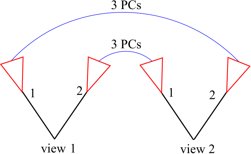
(a) Inter-camera case.

(b) Intra-camera case.

Figure 3: Relative pose estimation for two-camera rigs. Specifically, our goal is to determine the 6DOF relative pose while six PCs are observable by two views of a two-camera rig. (a) inter-camera case, (b) intra-camera case.

Tab. 1 also shows the statistics of the proposed minimal solvers for two-camera rigs. The observations are summarized as follows: (1) When $\mathcal{E}_{1}$ is employed, the inter-camera solver has up to $56$ complex solutions, and there are one-dimensional families of extraneous roots in the intra-camera case. (2) By employing both $\mathcal{E}_{1}$ and $\mathcal{E}_{2}$, the number of complex solutions obtained by both the inter-camera and intra-camera solvers is $48$. (3) Compared to the solvers using quaternion parameterization, the solvers using Cayley parameterization yield smaller eliminate templates. We adopt Cayley parameterization as our default choice. (4) When only $\mathcal{E}_{1}$ is used in the 6pt+quat+inter configuration, it is necessary to explicitly consider the inequality $q_{w}\neq 0$. Otherwise, one-dimensional extraneous roots exist. We account for this inequality utilizing the saturation method [29], which yields $112$ solutions with one-fold symmetry. (5) For the 6pt+cayl+inter configuration, compared to the solvers derived from both $\mathcal{E}_{1}$ and $\mathcal{E}_{2}$, the solvers solely derived from $\mathcal{E}_{1}$ yield smaller eliminate templates and exhibit better numerical stability. This phenomenon indicates that the number of basis might affect the numerical stability of the solvers, which has been previously observed in the literatures [5, 13].

4 Experiments

Table 2: Comparison of solver runtime for multi-camera systems (unit: $\mu s$).

Methods	17pt-Li [35]	8pt-Kneip [24]	6pt-Stewénius [46]	6pt-Our-generic	6pt-Our-inter56	6pt-Our-inter48	6pt-Our-intra
Runtime	43.3	102.0	3275.4	2447.4	1677.8	1449.4	1463.8

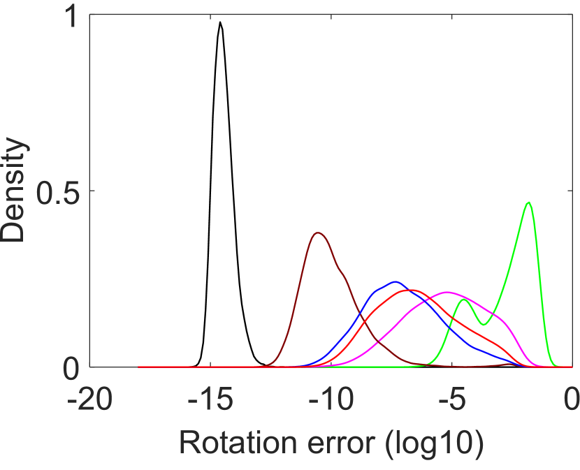
(a) Rotation error $\varepsilon_{\mathbf{R}}$.

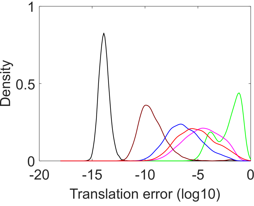
(b) Translation error $\varepsilon_{\mathbf{t}}$.

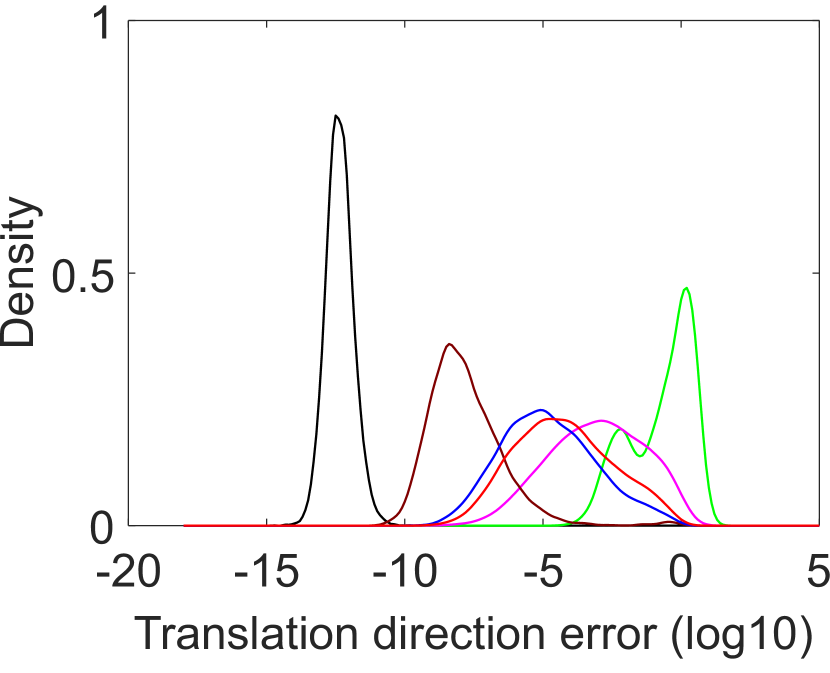
(c) Translation direction error $\varepsilon_{\mathbf{t},\text{dir}}$.

Figure 4: Probability density functions of the relative pose estimation error on noise-free observations. We designed a simulated two-camera rig comprising two perspective cameras. The orientations of two perspective cameras are roughly forward-facing with random perturbation. The horizontal axis corresponds to the $\log_{10}$ estimated errors, and the vertical axis is the empirical probability density.

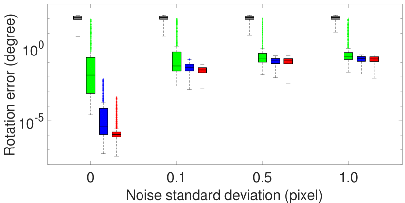
(a) ${\varepsilon_{\mathbf{R}}}$ in generic case.

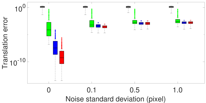
(b) $\varepsilon_{\mathbf{t}}$ in generic case.

(c) $\varepsilon_{\mathbf{t},\text{dir}}$ in generic case.

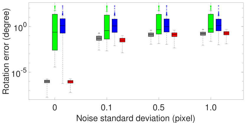
(d) ${\varepsilon_{\mathbf{R}}}$ in inter-camera case.

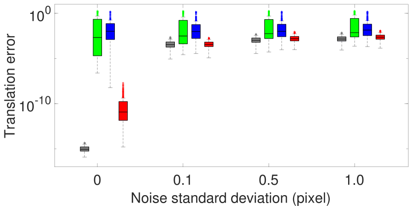
(e) $\varepsilon_{\mathbf{t}}$ in inter-camera case.

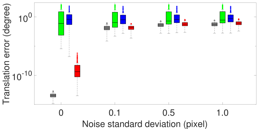
(f) $\varepsilon_{\mathbf{t},\text{dir}}$ in inter-camera case.

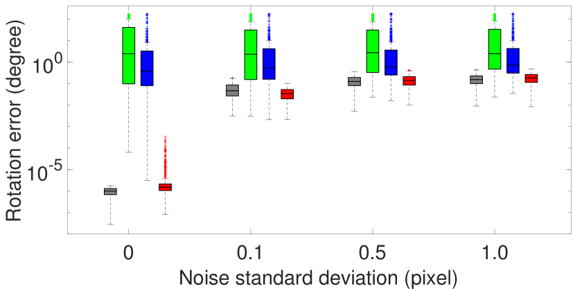
(g) ${\varepsilon_{\mathbf{R}}}$ in intra-camera case.

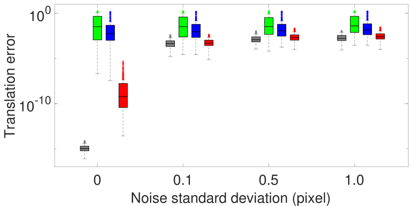
(h) $\varepsilon_{\mathbf{t}}$ in intra-camera case.

(i) $\varepsilon_{\mathbf{t},\text{dir}}$ in intra-camera case.

Figure 5: Relative pose estimation error with varying image noise for a generalized camera. We design a simulated multi-camera system comprising omnidirectional cameras. The extrinsic parameters, including orientation and position, are totally random. The three rows correspond to the generic, inter-camera, and intra-camera cases, respectively. The 6pt-Our solver in the three rows represent 6pt-Our-generic, 6pt-Our-inter, and 6pt-Our-intra, respectively.

This section presents a series of experiments performed on synthetic and real-world datasets to evaluate the performance of the proposed solvers. All the proposed solvers employ Cayley parameterization for their implementations. The solver presented in Sec. 3.4.1 is named as the 6pt-Our-generic method. The solvers proposed in Sec. 3.4.2, which aim to handle inter-camera and intra-camera cases, are named as the 6pt-Our-inter and 6pt-Our-intra solvers, respectively. To further differentiate between different solvers for 6pt-Our-inter, we denote the solvers resulting from ${\mathcal{E}}_{1}$ and ${\mathcal{E}}_{1}\cup{\mathcal{E}}_{2}$ as 6pt-Our-inter56 and 6pt-Our-inter48, respectively. Refer to [24, 13], the proposed solvers are evaluated against state-of-the-art solvers using PCs, including 17pt-Li [35], 8pt-Kneip [24], and 6pt-Stewénius [46]. The paper does not evaluate solvers that exploit the additional affine parameters besides PCs [15, 13] or utilize a prior for relative pose estimation [49, 50]. The proposed minimal solvers are implemented in C++. The source codes for the comparison methods are adopted from the OpenGV library [23].

In the experiments presented in Sec. 4.2 and Sec. 4.3, each solver is independently integrated into RANSAC [9] to reject outliers and obtain the estimated relative pose with the highest number of inliers. The angular re-projection error [23, 33] introduced by PCs is used to classify inliers. We follow the default parameters of OpenGV to set the inlier threshold angle as $0.1^{\circ}$ [23]. During RANSAC iterations, the outlier ratio is from the current best model. The stopping criterion of RANSAC iterations is that at least one outlier-free set is sampled with a probability $0.99$, or the maximum number $20,000$ of iterations is reached. We compute the rotation error as the angular difference between the ground truth rotation $\mathbf{R}_{\text{gt}}$ and the estimated rotation ${\mathbf{R}}$: ${\varepsilon_{\mathbf{R}}}=\arccos((\operatorname*{trace}({\mathbf{R}_{\text{gt}}}{{\mathbf{R}^{T}}})-1)/2)$. To calculate the translation error, we employ the definition introduced in [43, 32]: ${\varepsilon_{\mathbf{t}}}=2\left\|{{\mathbf{t}_{\text{gt}}}}-{\mathbf{t}}\right\|/(\left\|{\mathbf{t}_{\text{gt}}}\right\|+\left\|{{\mathbf{t}}}\right\|)$, where $\mathbf{t}_{\text{gt}}$ and ${\mathbf{t}}$ are the ground truth translation and the estimated translation, respectively. We also compute the translation direction error: $\varepsilon_{\mathbf{t},\text{dir}}=\arccos(\mathbf{t}_{\text{gt}}^{T}\mathbf{t}/(\|\mathbf{t}_{\text{gt}}\|\cdot\|\mathbf{t}\|))$.

The principles of minimal solver choice are listed below. First, when 6pt-Our-inter or 6pt-Our-intra are applicable, we apply them with higher priority than 6pt-Our-generic. The reason is that the solvers of specific configurations usually have better performance than the generic solver. Second, we recommend 6pt-Our-intra as the default solver for real-world image sequences. The relative pose is usually estimated for consecutive image pairs captured in a small time interval. Thus, intra-camera PCs can be built up with a higher probability than inter-camera PCs.

4.1 Efficiency and Numerical Stability

The runtimes of the solvers for multi-camera systems are assessed using an Intel(R) Core(TM) i7-7800X 3.50 GHz processor. The average runtime of the solvers over $10,000$ runs is shown in Tab. 2. As a linear solver, 17pt-Li is the most efficient one. All the proposed solvers have runtimes of $1.5\sim 2.5$ milliseconds, which are more efficient than the seminal 6pt-Stewénius among the minimal solvers.

To test the numerical stability, we design two simulated scenarios. First, we design a simulated two-camera rig composed of two perspective cameras. The orientations of the two perspective cameras are roughly forward-facing with random perturbation. This setting is practical for autonomous driving with two front-facing cameras. Second, we design a simulated generalized camera composed of omnidirectional cameras. The extrinsic parameters, including orientation and position, are totally random. We report the results for the solvers under the first scenario below. The results for generalized cameras under the second scenario are shown in the supplementary material.

Under the first scenario, the numerical stability of the solvers on noise-free observations is shown in Fig. 4. The procedure is repeated for $10,000$ times on both inter-camera and intra-camera cases. The resulting empirical probability density functions are represented as a function of the $\log_{10}$ estimated errors. The numerical stability of a solver is determined by many factors, such as the problem’s complexity, parameterization, equation system construction, solver generator, and implementation. Usually, more efficient solvers generated by effective methods have less round-off error and thus have better numerical stability. Among these solvers, the 17pt-Li solver demonstrates the best numerical stability due to its status as a linear solver with fewer computations. Since the 8pt-Kneip solver relies on iterative optimization, it is susceptible to becoming trapped in local minima. All the proposed solvers exhibit satisfactory numerical stability. Since the 6pt-Our-inter56 solver displays better numerical stability than the 6pt-Our-inter48 solver, we recommend 6pt-Our-inter56 as the default solver for inter-camera case in the follow-up experiments.

4.2 Experiments on Synthetic Data

Following Sec. 4.1, two simulated scenarios are designed and tested for the synthetic experiments, including scenarios for a two-camera rig and a generalized camera. The results for two-camera rigs under the first scenario are shown in the supplementary material.

Under the second scenario, the simulated scenario for a generalized camera is described as below. For the generic case, a generalized camera comprises 12 omnidirectional cameras. For the inter-camera and intra-camera cases, a generalized camera comprises 2 omnidirectional cameras. The extrinsic parameters of each omnidirectional camera are generated randomly. Each scene point is generated randomly. In addition, the relative poses between the two views are also generated randomly. Omnidirectional cameras are selected in our settings, because usually there is no overlap for pinhole cameras with random extrinsic parameters and relative poses. We test the accuracy of pose estimation for all the proposed solvers, including 6pt-Our-generic, 6pt-Our-inter, and 6pt-Our-intra solvers.

Some of the comparison solvers use more PCs than the proposed solvers. The strategy of correspondence selection has a significant influence on their performance. We design a rule to select matches for different cases to guarantee fairness. Please see the supplementary material for details. In the synthetic experiments, we conduct $1000$ trials for each case and a specific noise level combined with the RANSAC framework. For each trial, we randomly generate 100 PCs and select correspondences randomly for the different solvers. Fig. 5 illustrates the performance of various solvers against image noise for generalized cameras. The observations are summarized as follows: (1) 17pt-Li has good overall accuracy for inter-camera and intra-camera cases. However, it fails for the generic case due to rank deficiency, and the essential matrix with scale ambiguity cannot be uniquely recovered. (2) 8pt-Kneip has acceptable results according to the median metric. However, the error variance is large for all the cases. (3) 6pt-Stewénius has good overall accuracy for the generic case. It does not work well for inter-camera and intra-camera cases, and the error variance is large for both cases. This phenomenon is consistent with [22], which observes this solver does not work for most axial cameras where every bearing vector intersects a line in 3D. (4) The proposed 6pt-Our solver works for all the cases and has satisfactory overall accuracy.

4.3 Experiments on Real-World Data

To evaluate the performance of the proposed solvers in practical applications, three public datasets KITTI [10], nuScenes [6], and EuRoc [4] are used in the experiments. Specifically, the KITTI and nuScenes datasets are collected in autonomous driving environments, while the EuRoc dataset is collected in a micro aerial vehicle environment. These datasets contain challenging image pairs, such as highly dynamic scenes and significant motion. The proposed solvers are compared with state-of-the-art solvers. The accuracy of relative pose estimation is evaluated using the rotation error ${\varepsilon_{\bf{R}}}$ and the translation direction error $\varepsilon_{\mathbf{t},\text{dir}}$ [24, 37]. Our evaluation is based on approximately $30,000$ image pairs, and we report the final estimation results by integrating the minimal solver with RANSAC. The results for nuScenes and EuRoc datasets are provided in the supplementary material.

Table 3: Rotation and translation error on KITTI dataset (unit: degree).

Seq.	17pt-Li [35]	8pt-Kneip [24]	6pt-Stew. [46]	6pt-Our-intra
	${\varepsilon_{\bf{R}}}$  $\varepsilon_{\mathbf{t},\text{dir}}$	${\varepsilon_{\bf{R}}}$  $\varepsilon_{\mathbf{t},\text{dir}}$	${\varepsilon_{\bf{R}}}$  $\varepsilon_{\mathbf{t},\text{dir}}$	${\varepsilon_{\bf{R}}}$  $\varepsilon_{\mathbf{t},\text{dir}}$
00	0.147   2.537	0.148   2.496	0.259   4.938	0.136  2.415
01	0.178   4.407	0.182   3.485	0.303   7.557	0.175  3.323
02	0.142   1.988	0.147   2.094	0.228   3.474	0.139  1.897
03	0.126   2.762	0.139   2.833	0.327   6.324	0.143  2.740
04	0.113   1.733	0.123   1.829	0.269   3.770	0.101  1.677
05	0.132   2.663	0.130   2.461	0.225   4.404	0.128  2.342
06	0.139   2.146	0.151   2.145	0.203   3.258	0.121  2.064
07	0.131   3.085	0.172   3.259	0.264   6.831	0.129  2.904
08	0.133  2.705	0.135   2.762	0.228   4.914	0.140  2.620
09	0.144   2.022	0.138  1.974	0.212  3.246	0.126   2.002
10	0.142   2.398	0.141   2.393	0.249   4.155	0.137  2.314

Table 4: Average runtime of RANSAC on KITTI dataset (unit: $s$).

Methods	17pt-Li [35]	8pt-Kneip [24]	6pt-Stew. [46]	6pt-Our-intra
Mean time	3.157	0.648	4.723	1.849
Std. deviation	0.119	0.009	0.161	0.072

We evaluate all the solvers on KITTI dataset [10], which is collected using outdoor autonomous vehicles installed with forward-facing stereo cameras. It is treated as a general multi-camera system by ignoring overlapping fields of view for cameras. The 6pt-Our-intra solver is tested on 11 available sequences containing 23,000 image pairs. The ground truth is obtained directly from the GPS/IMU localization unit [10]. To establish PCs for consecutive views of each camera, the SIFT method [38] is used. Additionally, all the solvers are integrated into RANSAC to remove mismatches in the experiments.

Tab. 3 illustrates the rotation and translation error of the 6pt-Our-intra solver on KITTI dataset. We use median error to evaluate the performance of solvers. The proposed 6pt-Our-intra solver outperforms the comparative solvers in overall performance. To further compare computational efficiency, Tab. 4 illustrates the corresponding average runtime of RANSAC on KITTI dataset. Although 17pt-Li is faster than the proposed 6pt-Our-intra, the proposed solver demonstrates better efficiency when integrated them separately into the RANSAC framework.

5 Conclusion

We proposed a series of minimal solvers to compute the 6DOF relative pose of a multi-camera system using a minimal number of six PCs. We also exploit ray bundle constraints that allow for a reduction of the solution space and the development of more stable solvers. A generic solver is proposed for the relative pose estimation of generalized cameras. All configurations of minimal six-point problems for multi-camera systems are enumerated. Moreover, two minimal solvers, including an inter-camera solver and an intra-camera solver, are proposed for practical configurations of two-camera rigs. Based on synthetic and real-world experiments, we demonstrate that the proposed solvers offer an efficient solution for ego-motion estimation, surpassing state-of-the-art solvers in terms of accuracy.

Supplementary Material

6 Proof of a Common Factor

In Section 3.3 of the paper, we say that a factor $q_{x}^{2}+q_{y}^{2}+q_{z}^{2}+1$ can be factored out in Eqs. (16) and (17) of the paper. This property can be proven by symbolic computation using Matlab. The Matlab code is listed in LABEL:lst:proof.

Listing 1: Proof by Symbolic Computation using Matlab

⬇

%% define an orthogonal matrix via Cayley’s formula

syms x y z real

Q = [1+x^2-y^2-z^2, 2*x*y-2*z, 2*y+2*x*z; 2*x*y+2*z, 1-x^2+y^2-z^2, 2*y*z-2*x; 2*x*z-2*y, 2*x+2*y*z, 1-x^2-y^2+z^2];

%% check orthogonality

% The results are s^2*diag([1, 1, 1]),

% where s = x^2+y^2+z^2+1.

simplify(Q*Q’)

%%␣construct␣a␣3*3␣random␣matrix␣N␣in␣Eq.(17)

imax␣=␣10;

c␣=␣cell(3,␣1);

for␣i␣=␣1:3

␣␣c{i}␣=␣cross(randi(imax,␣[3,1]),␣Q*randi(imax,␣[3,1]));

end

C1␣=␣[c{1},␣c{2},␣c{3}];

eq1␣=␣det(C1);

%%␣check␣the␣determinant␣has␣factor␣x^2+y^2+z^2+1

factor(eq1)

%%␣construct␣a␣4*4␣random␣matrix␣N␣in␣Eq.(16)

c␣=␣cell(4,␣1);

mm␣=␣[x^2;␣y^2;␣z^2;␣x*y;␣x*z;␣y*z;␣x;␣y;␣z;␣1];

for␣i␣=␣1:4

␣␣tmp␣=␣randi(imax,␣[1,␣10])*mm;

␣␣c{i}␣=␣[cross(randi(imax,␣[3,1]),␣Q*randi(imax,␣[3,1]));␣tmp];

end

C2␣=␣[c{1},␣c{2},␣c{3},␣c{4}];

eq2␣=␣det(C2);

%%␣check␣the␣determinant␣has␣factor␣x^2+y^2+z^2+1

factor(eq2)

It can be seen that $3\times 3$ and $4\times 4$ submatrices of ${\mathbf{M}}(q_{x},q_{y},q_{z})$ in Eq. (9) of the paper have a common factor $q_{x}^{2}+q_{y}^{2}+q_{z}^{2}+1$. Thus, we can use this property to factor out $q_{x}^{2}+q_{y}^{2}+q_{z}^{2}+1$ to simplify the equation system in the paper. It will generate more efficient solvers and sometimes avoid false roots.

7 Configuration Enumeration for Six-Point Solvers

In Section 3.4 of the paper, two configurations called inter-camera and intra-camera are investigated for the six-point problem for two-camera rigs. Please refer to Fig. 3 in the paper. Then a question naturally appears as follows :

• How to enumerate all configurations of six-point problems for multi-camera systems?

7.1 Problem Definition

A configuration of point correspondences (PCs) can be modeled by a directed graph (also called digraph) by the following procedure. The vertex $i$ in the graph represents the single camera $i$ in a multi-camera system. An edge from vertex $i$ to $j$ in the graph represents a PC from camera $i$ in the first view to camera $j$ in the second view. For example, the inter-camera and intra-camera cases in the Fig. 3 in the paper can be represented by Fig. 6. Then enumerating all the configurations can be equivalently converted to a graphical enumeration problem [18].

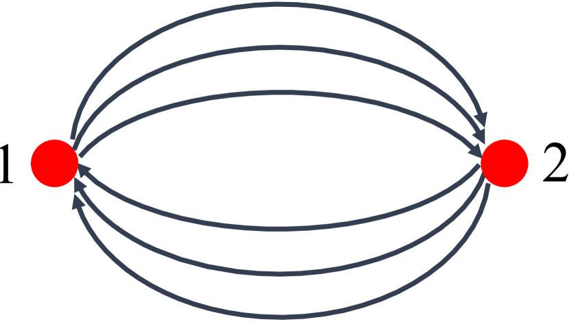
(a) Inter-camera case.

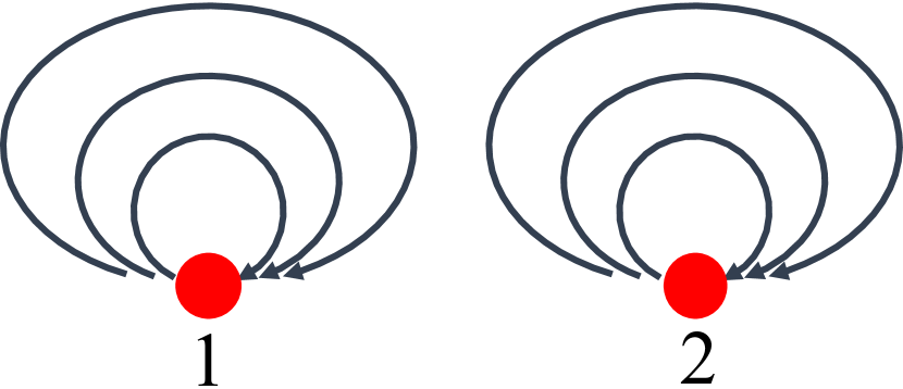
(b) Intra-camera case.

Figure 6: Directed graph representation of the inter-camera and intra-camera cases.

Problem Reformulation: We aim to count the $n$-edge directed graphs. The graphs do not have an isolated vertex. The graphs can contain loops (edges connecting a vertex to itself) and multiple edges (more than one edge connecting the same pair of vertices). How to count and enumerate distinct graphs for a given edge number $n$? Two graphs are distinct if and only if two conditions are met: (1) they are not isomorphic, (2) they cannot be converted to each other by reversing all edge directions of one graph. A graph $\mathcal{G}$ consists of a pair $(\mathcal{V},\mathcal{E})$, where $\mathcal{V}$ is the set of vertices and $\mathcal{E}$ the set of edges. In the paper, we are particularly interested in $n=6$, i.e., a minimal configuration of six PCs.

Isomorphism [Section 5 of [17]]: Two graphs $\mathcal{G}_{1}=(\mathcal{V}_{1},\mathcal{E}_{1})$ and $\mathcal{G}_{2}=(\mathcal{V}_{2},\mathcal{E}_{2})$ are isomorphic if there is a bijection $f:\mathcal{V}_{1}\to\mathcal{V}_{2}$ such that a directed edge $(u,v)\in\mathcal{E}_{1}$ if and only if $(f(u),f(v))\in\mathcal{E}_{2}$. In addition, the repetition numbers of $(u,v)$ and $(f(u),f(v))$ are the same if multiple edges or loops are allowed. This bijection $f$ is called an isomorphism.

Edge-Reversion Symmetry: This is a non-standard symmetry which is meaningful in our problem. A solver is applicable to a relative pose estimation problem whether it can determine the relative pose from view 1 to view 2 or from view 2 and view 1.

In the reformulated problem, the graph isomorphism is used to exclude the symmetry of camera indices. In other words, swapping camera indices do not change the configuration. The edge-reversion symmetry is used to exclude the symmetry of two views. A directed graph $\mathcal{G}$ with edges $\mathcal{E}=\{(u_{i},v_{i})\}_{i=1}^{n}$ and no isolated vertex can be represented by

$$E=\left[\begin{array}[]{cccc}u_{1}& u_{2}& \cdots& u_{n}\\ v_{1}& v_{2}& \cdots& v_{n}\end{array}\right]_{2\times n}$$ (20)

It is obvious that rearranging columns does not change the graph at all. In addition, a permutation of vertices in $E$ causes an isomorphic graph. Swapping two rows corresponds to reversing edge directions of this graph. In this paper, we write $E_{1}\cong E_{2}$ if $E_{2}$ can be obtained by rearrangement of columns, swapping rows, and swapping vertices of $E_{1}$.

Explanation of Isomorphism and Reversion Symmetry: When the first row is $\{1,2,3\}$ and the second row contain $\{1,2,3\}$, there are $6$ permutations, including

$$E_{1}=\left[\begin{array}[]{ccc}1& 2& 3\\ 1& 2& 3\end{array}\right],\ \ E_{2}=\left[\begin{array}[]{ccc}1& 2& 3\\ 1& 3& 2\end{array}\right],$$

$$E_{3}=\left[\begin{array}[]{ccc}1& 2& 3\\ 2& 1& 3\end{array}\right],\ \ E_{4}=\left[\begin{array}[]{ccc}1& 2& 3\\ 2& 3& 1\end{array}\right],$$

$$E_{5}=\left[\begin{array}[]{ccc}1& 2& 3\\ 3& 1& 2\end{array}\right],\ \ E_{6}=\left[\begin{array}[]{ccc}1& 2& 3\\ 3& 2& 1\end{array}\right].$$

It can be verified that $E_{3}$ can be convert to $E_{2}$ by swapping vertices $1$ and $3$; $E_{6}$ can be convert to $E_{2}$ by swapping vertices $1$ and $2$. $E_{5}$ can be convert to $E_{4}$ by swapping its two rows. As a result, there are $3$ distinct graph. The distinct graphs with isomorphism and edge-reversion symmetry are $E_{1}$, $E_{2}\cong E_{3}\cong E_{6}$, and $E_{4}\cong E_{5}$.

7.2 A Combinatorics Solution to Enumeration

Table 5: The number $D_{n}$ of distinct graphs given $n$ edges.

#edge $n$	1	2	3	4	5	6	7	8	9	10
#distinct graph	2	9	37	186	985	5953	38689	271492	2016845	15767277

Table 6: The number of cases for different camera numbers given $6$ edges. Totally there are $5953$ cases.

#camera	1	2	3	4	5	6	7	8	9	10	11	12
#cases	1	29	270	1029	1776	1630	853	280	66	15	3	1

Table 7: The number of cases for different camera numbers given $7$ edges. Totally there are $38689$ cases.

#camera	1	2	3	4	5	6	7	8	9	10	11	12	13	14
#cases	1	39	568	3316	8599	11516	8787	4170	1296	312	66	15	3	1

The problem is related to combinatorics and group theory. When isomorphism without edge-reversion symmetry is considered in multigraph enumeration, the problem has been investigated in [41]. However, when edge-reversion symmetry is also considered, little study has been investigated. The Pólya Enumeration Theorem can be applied to solve this problem [17]. To apply this theorem, we need to generate the cycle index of the permutation group $S_{n}$ acting on $n$ elements. Then we obtain the number of isomorphic graphs from this cycle index of $S_{n}$.

In addition to theoretical analysis, we can enumerate all the distinct graphs in a recursive way by computer programming. We use about $50$ lines of Matlab codes to determine the distinct graphs, as shown in LABEL:lst:graph.

Listing 2: Generate Distinct Graphs Using Matlab

⬇

function G_curr = generate_distict_graph(edge_num)

G_curr = {};

for k = 1:edge_num

G_prev = G_curr;

G_curr = generate_graph_recursion(G_prev, k);

end

function G_curr = generate_graph_recursion(G_prev, k)

if k == 1

G_curr = cell(1, 2);

G_curr{1} = struct(’E’,␣[1;␣1]);

␣␣G_curr{2}␣=␣struct(’E’,␣[1;␣2]);

␣␣return;

end

curr_sz␣=␣0;

G_curr␣=␣{};

for␣i␣=␣1:numel(G_prev)

␣␣E0␣=␣G_prev{i}.E;

␣␣edge_all␣=␣generate_edge_set(E0);

␣␣for␣j␣=␣1:size(edge_all,␣2)

␣␣␣␣E␣=␣[E0,␣edge_all(:,␣j)];

␣␣␣␣G␣=␣digraph(E(1,␣:),␣E(2,␣:));

␣␣␣␣H␣=␣digraph(E(2,␣:),␣E(1,␣:));

␣␣␣␣if␣~is_in_set(G,␣H,␣G_curr,␣curr_sz)

␣␣␣␣␣curr_sz␣=␣curr_sz␣+␣1;

␣␣␣␣␣G_curr{curr_sz}␣=␣struct(’E’,␣E,␣’G’,␣G);

␣␣␣␣end

␣␣end

end

fprintf(’#edge:␣%d,␣#found-graphs:␣%d\n’,␣k,␣curr_sz);

function␣edge_all␣=␣generate_edge_set(E)

s0␣=␣unique(E(:));

s␣=␣[s0(:);␣max(s0)+1];

n␣=␣numel(s);

edge_all␣=␣zeros(2,␣n*n+1);

i1␣=␣kron(1:n,␣ones(1,n));

i2␣=␣kron(ones(1,n),␣1:n);

edge_all(:,␣1:n^2)␣=␣[s(i1),␣s(i2)]’;

edge_all(:,␣end)␣=␣max(s0)+[1;␣2];

function␣flag␣=␣is_in_set(G,␣H,␣G_set,␣curr_sz)

flag␣=␣false;

␣␣for␣ii␣=␣1:curr_sz

␣␣␣␣G1␣=␣G_set{ii}.G;

␣␣␣␣if␣(isisomorphic(G1,␣G)␣||␣isisomorphic(G1,␣H))

␣␣␣␣␣␣flag␣=␣true;

␣␣␣␣return;

␣␣end

end

7.3 Statistics of Cases and Solvers

The number $D_{n}$ of distinct graphs for different edge numbers $n$ are shown in Tab. 5. When $n=6$ and $7$, the number of cases for different camera numbers are shown in Tab. 6 and Tab. 7, respectively.

Since this paper focuses on six-point methods, we are particularly interested in the situation of $n=6$. When $n=6$, we classify its $5953$ cases into $6$ match types as below.

• Match type $6\cup\phi$: All the 6 edges are same. There are $2$ cases belong to this match type, including

  $$E_{1}=\left[\begin{array}[]{cccccc}1& 1& 1&1&1&1\\ 1& 1& 1&1&1&1\end{array}\right],$$

  $$E_{2}=\left[\begin{array}[]{cccccc}1& 1& 1&1&1&1\\ 2& 2& 2&2&2&2\end{array}\right].$$

  These two cases essentially correspond to monocular cameras. Since $6$ PCs provide an over-determined equation system, the equation system has none solution.

• Match type $5\cup x$: The maximal repetitive number of multiple edges is $5$. For example,

  $$E_{3}=\left[\begin{array}[]{cccccc}1& 1& 1&1&1&2\\ 1& 1& 1&1&1&3\end{array}\right].$$

• Match type $4\cup x$: The maximal repetitive number of multiple edges is $4$. For example,

  $$E_{4}=\left[\begin{array}[]{cccccc}1& 1& 1&1&2&4\\ 1& 1& 1&1&3&5\end{array}\right].$$

• Match type $3\cup 3$: The maximal repetitive number of multiple edges is $3$, and there are two multiple edges satisfying this condition. For example, the previously defined inter-camera and intra-camera cases belong to this match type. They are

  $$E_{5}=\left[\begin{array}[]{cccccc}1& 1& 1&2&2&2\\ 2& 2& 2&1&1&1\end{array}\right],$$

  $$E_{6}=\left[\begin{array}[]{cccccc}1& 1& 1&2&2&2\\ 1& 1& 1&2&2&2\end{array}\right].$$

• Match type $3\cup x$: The maximal repetitive number of multiple edges is $3$, and there are only one multiple edge satisfying this condition. For example,

  $$E_{7}=\left[\begin{array}[]{cccccc}1& 1& 1&2&4&6\\ 1& 1& 1&3&5&7\end{array}\right].$$

• Match type $\cup_{i}x_{i}$: The maximal repetitive number of multiple edges is less or equal than $2$. For example,

  $$E_{8}=\left[\begin{array}[]{cccccc}1& 3& 5&7&9&11\\ 2& 4& 6&8&10&12\end{array}\right].$$

  Most of the cases belong to this match type. In the previous section, we call it the generic case.

For different match types, the numbers of equations in $\mathcal{E}_{1}$ and $\mathcal{E}_{2}$ are different. We found that cases belong to the same match type have preciously the same number of solutions. Tab. 8 shows the number of solutions for different match types in six-point problems for multi-camera systems.

Table 8: The number of solutions and the number of solvers for different match types when $n=6$. Totally there are $5953$ cases.

match type	$6\cup\phi$	$5\cup x$	$4\cup x$	$3\cup 3$	$3\cup x$	$\cup_{i}x_{i}$
#case	2	9	63	7	412	5460
#equ. in $\mathcal{E}_{1}$	0	10	14	15	15	15
#equ. in $\mathcal{E}_{2}$	20	10	4	2	1	0
#solution	0	20	40	48	56	64

8 Experiments

In this section, we add more experiments about the 6DOF relative pose estimation of a multi-camera system. As described in the paper, all the solvers are implemented in C++. The source codes of the comparison methods are taken from the OpenGV library [23]. The numerical stability of the proposed solvers under the second simulated scenario is shown in Sec. 8.1. Expected runtime vs. inlier ratio accounting for numerical stability is demonstrated in Sec. 8.2. More experiments on synthetic data are shown in Sec. 8.3. The real-world experiments on KITTI, nuScenes, and EuRoC datasets are shown in Sec. 8.4, Sec. 8.5 and Sec. 8.6, respectively.

8.1 Numerical Stability

In Section 4.1 of the paper, we design two simulated scenarios to test the numerical stability. First, we design a simulated two-camera rig composed of two perspective cameras. The orientations of the two perspective cameras are roughly forward-facing with random perturbation. This setting is practical for autonomous driving with two front-facing cameras. Second, we design a simulated generalized camera composed of omnidirectional cameras. The extrinsic parameters, including orientation and position, are totally random. We report the results for the solvers under the first scenario below in the paper. The results for generalized cameras under the second scenario are shown in the supplementary material.

Fig. 7 reports the numerical stability of the solvers on noise-free observations under the second scenario. The numerical stability of the solvers is tested in generic-camera, inter-camera, and intra-camera configurations. The strategy of correspondence selection is described in Sec. 8.3.2. For all three cases, the proposed solvers have satisfactory numerical stability. Among them, the 6pt-Our-inter56 solver has the best numerical stability. None of the comparison solvers can have satisfactory results for all the cases. Specifically,

• 17pt-Li has satisfactory results for inter-camera and intra-camera cases. It does not work for generic case, because the essential matrix with scale ambiguity cannot be uniquely recovered due to the rank deficiency of the coefficient matrix. It can be proved by integer observations as that in [22]. Thus, it is not surprising that the corresponding numerical stability is extraordinarily bad.

• 8pt-Kneip does not have satisfactory results. The ground truth of rotation is random in the experiment settings, and this solver uses an identity matrix to initialize the rotation. As a result, its solutions determined by local optimization are prone to local minima.

• 6pt-Stewénius has satisfactory results for generic-camera configuration. However, due to their bad numerical stability, they do not work well for inter-camera and intra-camera cases. This phenomenon is consistent with [22], which observes the 6pt-Stewénius solver does not work for most axial cameras.

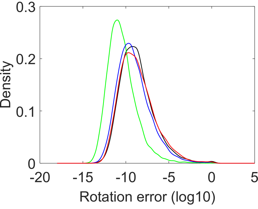
(a) Rotation error $\varepsilon_{\mathbf{R}}$.

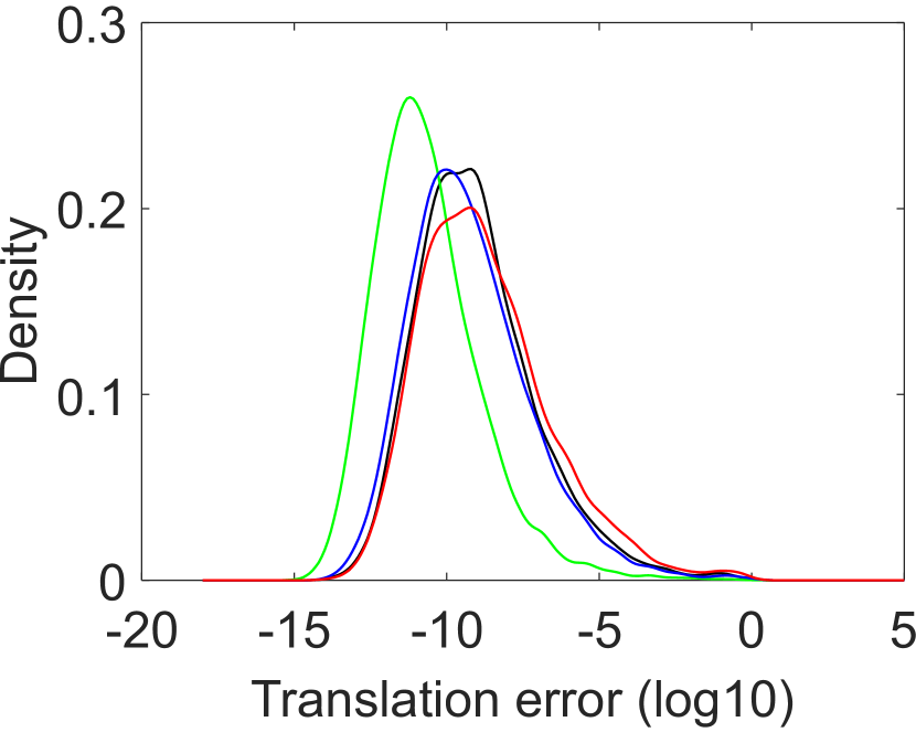
(b) Translation error $\varepsilon_{\mathbf{t}}$.

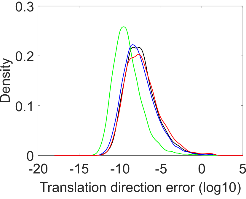
(c) Translation direction error $\varepsilon_{\mathbf{t},\text{dir}}$.

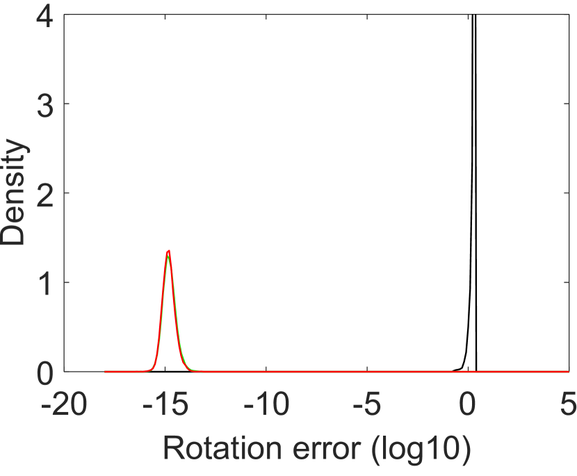
(d) Rotation error $\varepsilon_{\mathbf{R}}$.

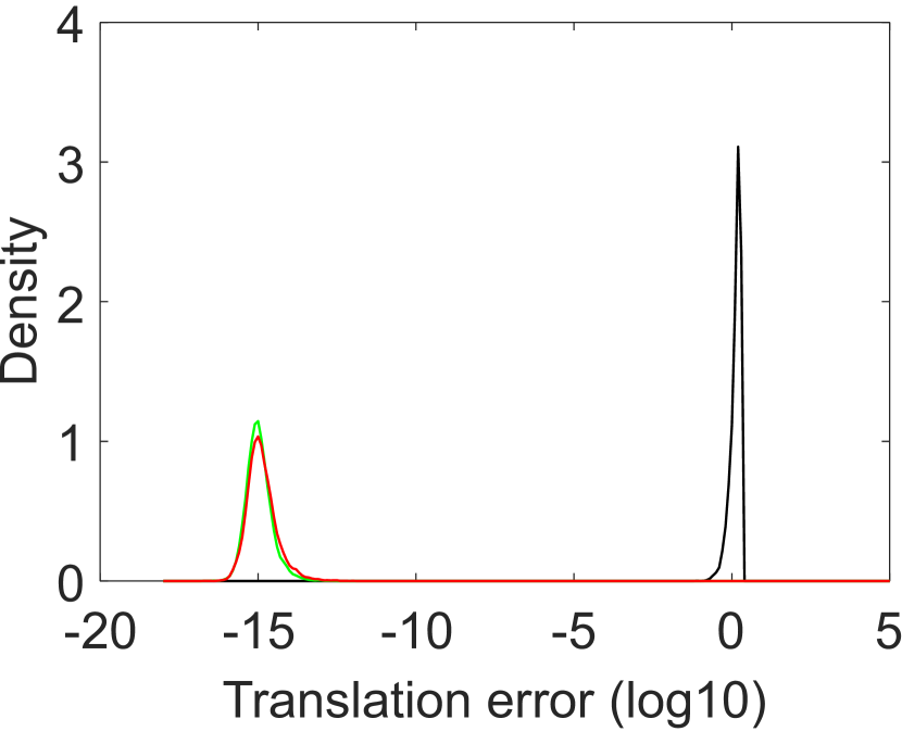
(e) Translation error $\varepsilon_{\mathbf{t}}$.

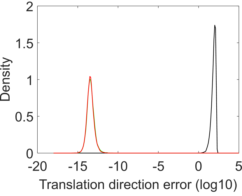
(f) Translation direction error $\varepsilon_{\mathbf{t},\text{dir}}$.

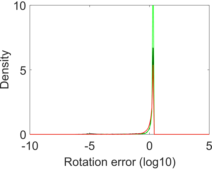
(g) Rotation error $\varepsilon_{\mathbf{R}}$.

(h) Translation error $\varepsilon_{\mathbf{t}}$.

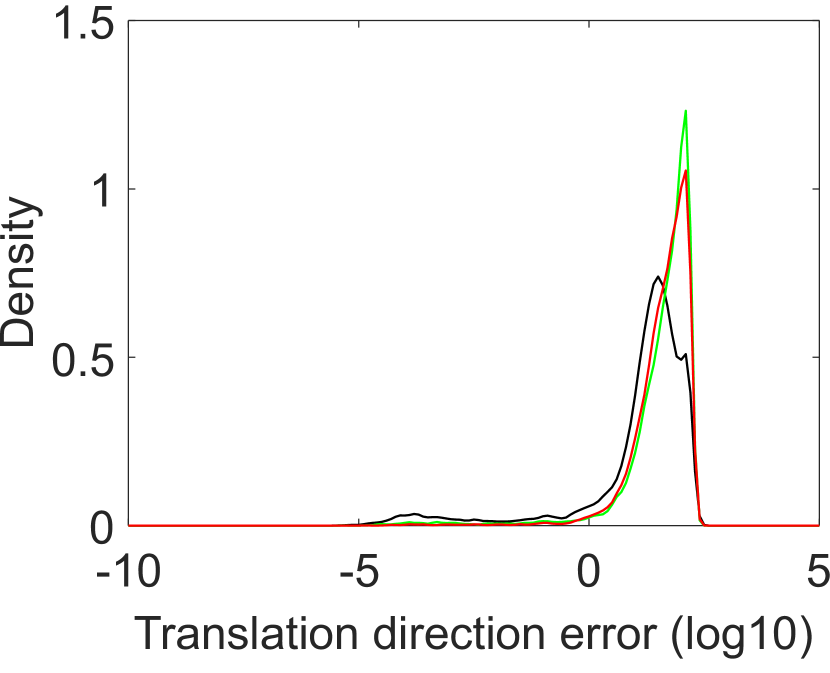
(i) Translation direction error $\varepsilon_{\mathbf{t},\text{dir}}$.

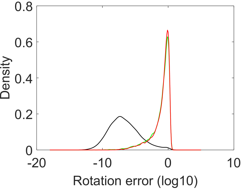
(j) Rotation error $\varepsilon_{\mathbf{R}}$.

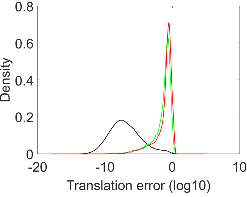
(k) Translation error $\varepsilon_{\mathbf{t}}$.

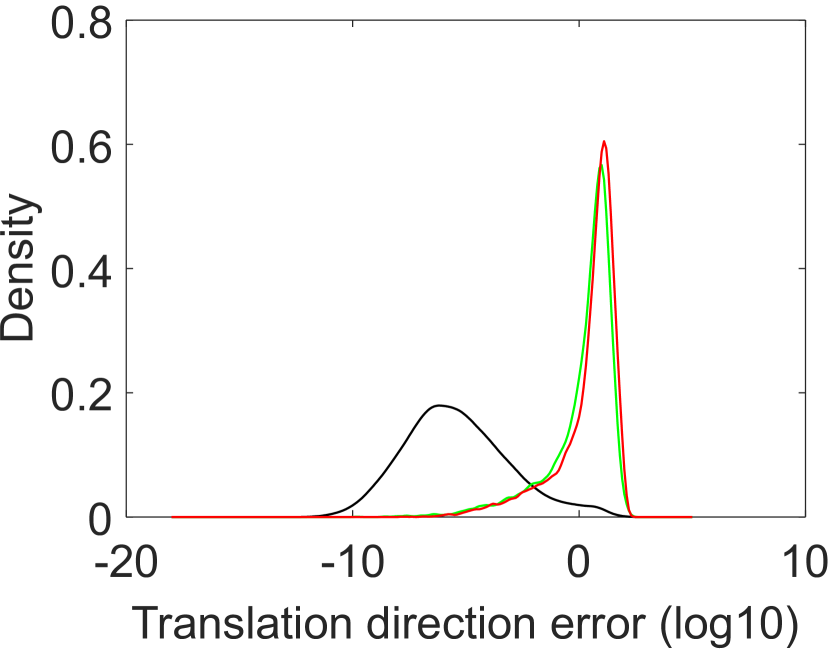
(l) Translation direction error $\varepsilon_{\mathbf{t},\text{dir}}$.

Figure 7: Probability density functions over pose estimation errors on noise-free observations for the proposed solvers. We design a simulated multi-camera system composed of twelve omnidirectional cameras. The extrinsic parameters, including orientation and position, are totally random. The horizontal axis represents the $\log_{10}$ errors, and the vertical axis represents the density.

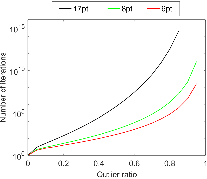
(a) Iteration number without accounting for numerical stability.

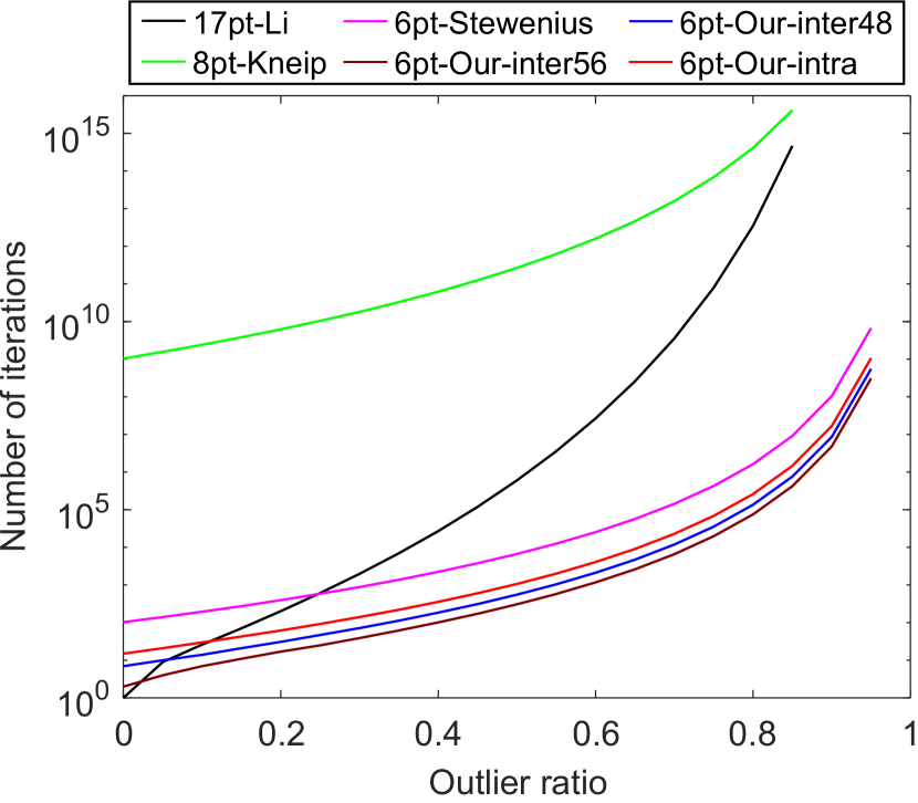
(b) Iteration number accounting for numerical stability.

Figure 8: RANSAC iteration number with respect to outlier ratio for success probability $99\%$.

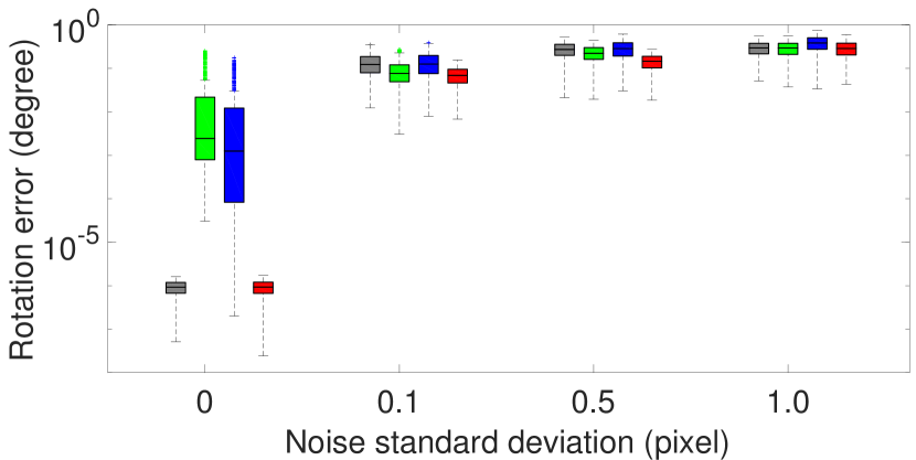
(a) ${\varepsilon_{\mathbf{R}}}$ for forward motion.

(b) $\varepsilon_{\mathbf{t}}$ for forward motion.

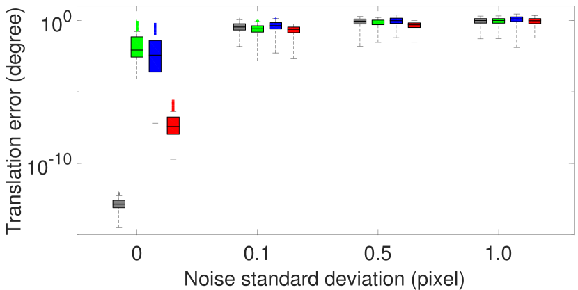
(c) $\varepsilon_{\mathbf{t},\text{dir}}$ for forward motion.

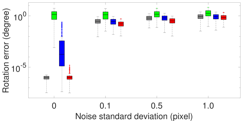
(d) ${\varepsilon_{\mathbf{R}}}$ for sideways motion.

(e) $\varepsilon_{\mathbf{t}}$ for sideways motion.

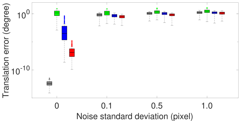
(f) $\varepsilon_{\mathbf{t},\text{dir}}$ for sideways motion.

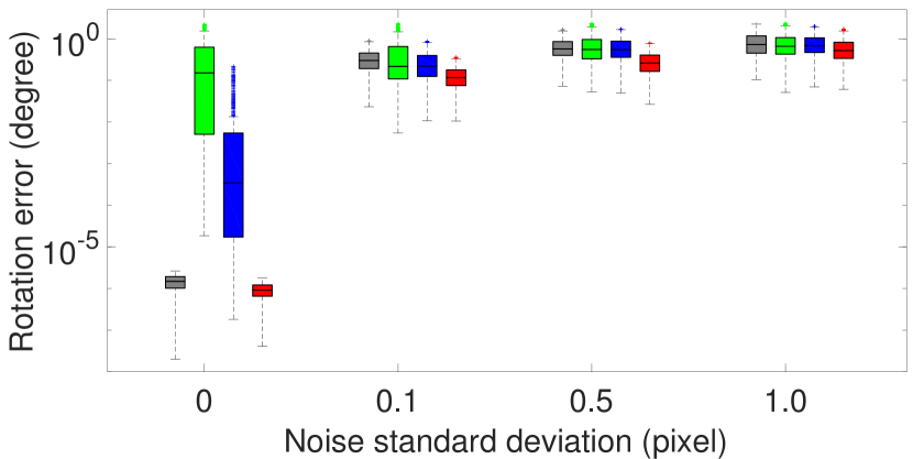
(g) ${\varepsilon_{\mathbf{R}}}$ for random motion.

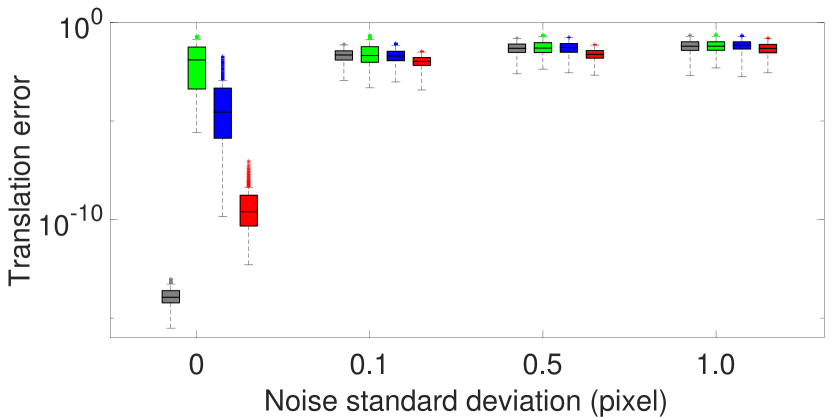
(h) $\varepsilon_{\mathbf{t}}$ for random motion.

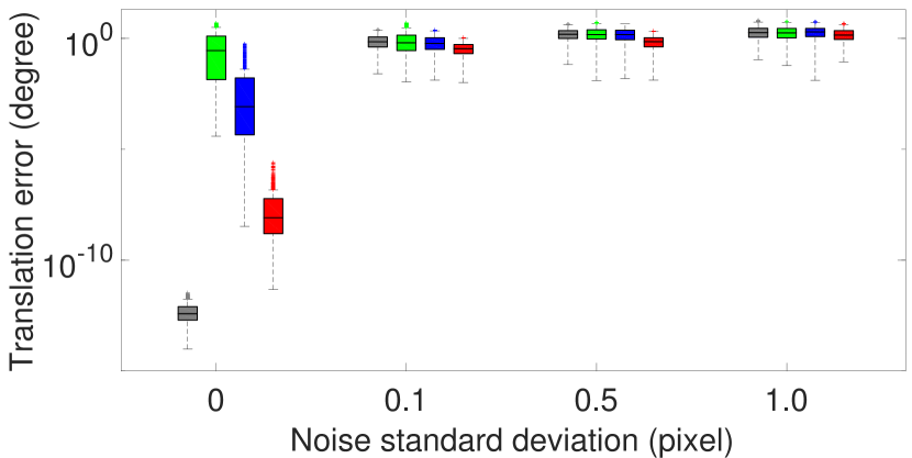
(i) $\varepsilon_{\mathbf{t},\text{dir}}$ for random motion.

Figure 9: Rotation and translation error with varying image noise for the inter-camera case. We designed a simulated two-camera rig composed of two perspective cameras. The orientations of the two perspective cameras are roughly forward-facing with random perturbation. The three rows correspond to forward, sideways, and random motions, respectively.

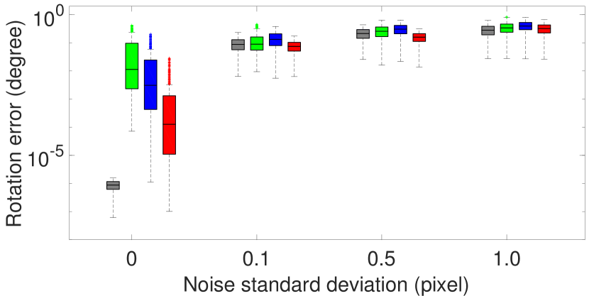
(a) ${\varepsilon_{\mathbf{R}}}$ for forward motion.

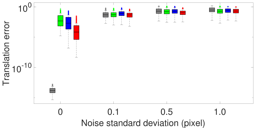
(b) $\varepsilon_{\mathbf{t}}$ for forward motion.

(c) $\varepsilon_{\mathbf{t},\text{dir}}$ for forward motion.

(d) ${\varepsilon_{\mathbf{R}}}$ for sideways motion.

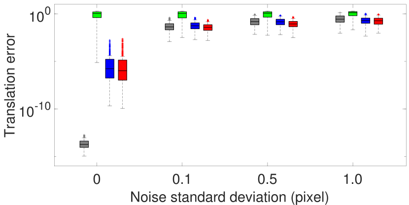
(e) $\varepsilon_{\mathbf{t}}$ for sideways motion.

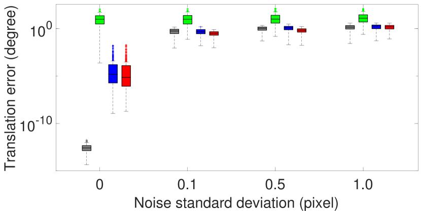
(f) $\varepsilon_{\mathbf{t},\text{dir}}$ for sideways motion.

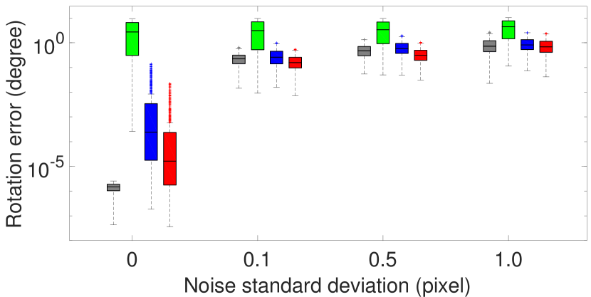
(g) ${\varepsilon_{\mathbf{R}}}$ for random motion.

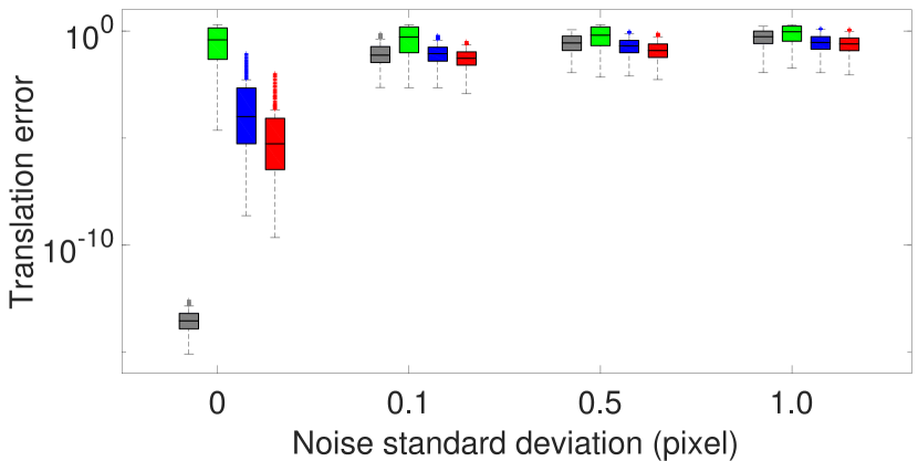
(h) $\varepsilon_{\mathbf{t}}$ for random motion.

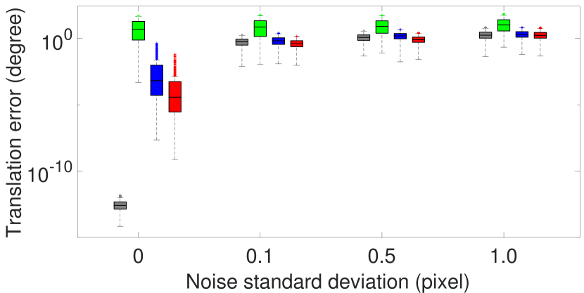
(i) $\varepsilon_{\mathbf{t},\text{dir}}$ for random motion.

Figure 10: Rotation and translation error with varying image noise for the intra-camera case. We designed a simulated two-camera rig composed of two perspective cameras. The orientations of the two perspective cameras are roughly forward-facing with random perturbation. The three rows correspond to forward, sideways, and random motions, respectively.

8.2 Expected Runtime vs. Inlier Ratio Accounting for Numerical Stability

The runtime of RANSAC depends on the runtime of the minimal solver and iteration number. For the RANSAC methods, the iteration number is determined by the probability of choosing at least one inlier set. This calculation implicitly assumes that an accurate solution can be obtained given an inlier set. However, this is not always true when considering the numerical stability of the minimal solvers.

Denote $p$ is the probability (usually set to 0.99) that at least one inlier set is sampled. $n$ is the minimum number of required data points in the minimal solver. For example, $s=6$ for the six-point solvers and $s=17$ for the 17-point solver. $\epsilon$ is the outlier ratio, i.e., the probability that any selected data point is an outlier. $N$ is the iteration number of RANSAC. In $N$ sampling times, the failure probability (one or more outliers are sampled in every sampling) is

$$(1-(1-\epsilon)^{s})^{N}=1-p,$$ (21)

and

$$N=\frac{\log(1-p)}{\log(1-(1-\epsilon)^{s})}.$$ (22)

When considering numerical stability, suppose $p_{2}$ is the probability of obtaining a sufficiently accurate solution given an inlier set. In $\hat{N}$ sampling times, the failure probability accounting for numerical stability is

$$(1-(p_{2}(1-\epsilon))^{s})^{\hat{N}}=1-p,$$ (23)

and

$$\hat{N}=\frac{\log(1-p)}{\log(1-(p_{2}(1-\epsilon))^{s})}.$$ (24)

Since $p_{2}\in[0,1]$ as a probability, we have $\hat{N}\geq N$ when accounting for numerical stability.

The left question is how to determine $p_{2}$ for a given minimal solver. For each minimal solver, we can empirically obtain the probability that the estimation errors $\varepsilon_{\mathbf{R}}$ and $\varepsilon_{\mathbf{t}}$ on noise-free observations are below specified thresholds. In this paper, we set the thresholds as $10^{-3}$. For the solvers 17pt-Li [35], 8pt-Kneip [24], 6pt-Stewénius [46], 6pt-Our-inter56, 6pt-Our-inter48 and 6pt-Our-intra, $p_{2}$ can be computed as 1.00, 0.09, 0.59, 0.99, 0.90 and 0.81, respectively. Fig. 8 shows RANSAC iteration numbers with respect to outlier ratio for success probability $99\%$.

8.3 Experiments on Synthetic Data

Following the experiments about numerical stability, two simulated scenarios are designed and tested for the synthetic experiments, including scenarios for a two-camera rig and a generalized camera. The proposed solvers are compared with state-of-the-art solvers including 17pt-Li [35], 8pt-Kneip [24], and 6pt-Stewénius [46].

8.3.1 Synthetic Experiments for Two-camera Rigs

In this scenario, we design a simulated two-camera rig composed of two perspective cameras. The orientations of the two perspective cameras are roughly forward-facing with random perturbation. This setting is practical for autonomous driving with two front-facing cameras [10]. The performance of the solvers are tested in inter-camera and intra-camera configurations. The baseline length between the two simulated cameras is set to $1$ meter. The multi-camera reference frame is defined at the middle of the camera rig, and the translation between two multi-camera reference frames is $3$ meters. The resolution of the cameras is $640\times 480$ pixels, and the focal lengths are $400$ pixels. The principal points are set to the image center. The synthetic scene is made up of a ground plane and $50$ random planes. These planes are randomly generated in a cube of $[-5,5]\times[-5,5]\times[10,20]$ meters, which are expressed in the respective axis of the multi-camera reference frame. We randomly choose $50$ PCs from the ground plane and a PC from each random plane. Thus, there are $100$ PCs generated randomly in the synthetic data.

A total of $1000$ trials are carried out in the synthetic experiment. In each trial, $100$ PCs are generated randomly. Correspondences for the different methods are selected randomly. The error is measured on the best relative pose, which produces the most inliers within the RANSAC scheme. The RANSAC scheme also allows us to select the best candidate from multiple solutions. The median of errors is used to assess the rotation and translation errors. In this set of experiments, the translation direction between two multi-camera references is chosen to produce forward, sideways, or random motions. For each motion, the second view is perturbed by a random rotation. This random rotation is rotated around three axes in order, and the rotation angles range from $-10^{\circ}$ to $10^{\circ}$.

Fig. 9 demonstrates the performance of different solvers against image noise for the inter-camera case. A good method should have small median and variance for ${\varepsilon_{\mathbf{R}}}$, ${\varepsilon_{\mathbf{t}}}$, and $\varepsilon_{\mathbf{t},\text{dir}}$. We have the following observations. (1) The proposed 6pt-Our-inter solver provides better results than the comparative solvers. (2) The iterative optimization in 8pt-Kneip is susceptible to falling into local minima. It performs well for forward and random motions. However, it does not perform well for the sideways motion. (3) The linear solver 17pt-Li with fewer calculations have less round-off error than the proposed 6pt-Our-inter solver in noise-free cases. However, our method has better accuracy than the linear solver with the influence of image noise. This is also consistent with real-world data experiments.

Fig. 10 demonstrates the performance of different solvers against image noise for the intra-camera case. We have the following observations. (1) Compared to the results in Fig. 9, the solvers using intra-camera correspondences generally perform worse than inter-camera correspondences, especially in recovering the metric scale of translation. (2) The proposed 6pt-Our-intra solver has better performance than the comparative solvers. (3) The 8pt-Kneip performs well in the forward motion of the multi-camera systems but poorly in the sideways and random motions.

8.3.2 Synthetic Experiments for Generalized Camera

Table 9: The correspondence selection for different solvers. The pair $(i,i^{\prime})$ represents a PC that appears in the $i$-th camera in the first view and the $i^{\prime}$-th camera in the second view. The multiplier after a pair means the number of this match type.

17pt-Li [35]	8pt-Kneip [24]	6pt-Stewénius [46]	6pt-Our-generic
(1,2)*3	(1,2)*2	(1,2)*1	(1,2)*1
(3,4)*3	(3,4)*2	(3,4)*1	(3,4)*1
(5,6)*3	(5,6)*1	(5,6)*1	(5,6)*1
(7,8)*3	(7,8)*1	(7,8)*1	(7,8)*1
(9,10)*3	(9,10)*1	(9,10)*1	(9,10)*1
(11,12)*2	(11,12)*1	(11,12)*1	(11,12)*1

In this scenario, we design a simulated generalized camera composed of 12 omnidirectional cameras. The extrinsic parameters, including orientation and position, are totally random. Some of the comparison solvers use more PCs than the proposed solvers. The strategy of correspondence selection has a significant influence on their performance. We design a rule to select matches for different cases to guarantee fairness. Take the generic-camera configuration as an example. The match types are $(1,2)$, $(3,4)$, $(5,6)$, $(7,8)$, $(9,10)$, and $(11,12)$ for the proposed generic solver. Recall that pair $(i,i^{\prime})$ represents a PC that appears in the $i$-th camera in the first view and the $i^{\prime}$-th camera in the second view. Solvers 17pt-Li, 8pt-Kneip, and 6pt-Stewénius cyclically build matches according to the order of $(1,2)$, $(3,4)$, $(5,6)$, $(7,8)$, $(9,10)$, and $(11,12)$. Tab. 9 shows the correspondence selection for different solvers.

8.4 Experiments on KITTI Dataset

The empirical cumulative error distributions for KITTI sequence 00 are shown in Fig. 11. These values are calculated from the same values which were used for creating Table 3 in the paper. It can be seen that the proposed 6pt-Our-intra solver offers the best overall performance in comparison to state-of-the-art solvers.

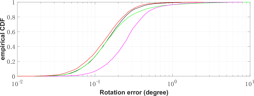
(a) Rotation error.

(b) Translation error.

Figure 11: Empirical cumulative error distributions for KITTI sequence 00.

8.5 Experiments on nuScenes Dataset

The performance of the solvers is also tested on the nuScenes dataset [6], which consists of consecutive keyframes from 6 cameras. This multi-camera system provides a full 360-degree field of view. We utilize all the keyframes of Part 1 for the evaluation, and there are 3376 images in total. The ground truth is given by a lidar map-based localization scheme. Similar to the experiments on KITTI dataset, the SIFT detector [38] is used to establish the PCs between consecutive views in six cameras. All the solvers are integrated into RANSAC to remove outlier matches of the feature correspondences.

Table 10: Rotation and translation error on nuScenes sequences (unit: degree).

Part	17pt-Li [35]	8pt-Kneip [24]	6pt-Stew. [46]	6pt-Our-intra
	${\varepsilon_{\bf{R}}}$  $\varepsilon_{\mathbf{t},\text{dir}}$	${\varepsilon_{\bf{R}}}$  $\varepsilon_{\mathbf{t},\text{dir}}$	${\varepsilon_{\bf{R}}}$  $\varepsilon_{\mathbf{t},\text{dir}}$	${\varepsilon_{\bf{R}}}$  $\varepsilon_{\mathbf{t},\text{dir}}$
01	0.183  2.826	0.175   2.732	0.214   2.978	0.155  2.519

Tab. 10 shows the rotation and translation error of the proposed 6pt-Our-intra for the Part1 of nuScenes dataset. The median error is used to evaluate the estimation accuracy. It is demonstrated that the proposed 6pt-Our-intra offers the best performance among all the methods. In comparison with experiments on KITTI dataset, this experiment also demonstrates that 6pt-Our-intra can be directly used for the relative pose estimation for the systems with more cameras.

8.6 Experiments on EuRoC Dataset

We further validate the proposed solvers in an unmanned aerial vehicle environment. The EuRoC MAV dataset [4] is used to evaluate the performance of 6DOF relative pose estimation, which is recorded using a stereo camera mounted on a micro aerial vehicle. The sequences labeled from MH01 to MH05 are collected in a large industrial machine hall. The ground truth of relative pose is provided from the nonlinear least-squares batch solution over the Leica position and IMU measurements. The relative pose estimation of these sequences is challenging, because the industrial environment is unstructured and cluttered. Considering that the movement of the consecutive image pair is small, the image pairs for relative pose estimation are thinned out by an amount of one out of every four consecutive images. We also exclude the image pairs with insufficient motion in this experiment. The proposed solvers are compared with state-of-the-art solvers including 17pt-Li [35], 8pt-Kneip [24], and 6pt-Stewénius [46]. The SIFT detector [38] is used to establish the PCs of the image pair. All the solvers are integrated into the RANSAC framework to remove mismatches.

Table 11: Rotation and translation error on EuRoC sequences (unit: degree).

Seq.	17pt-Li [35]	8pt-Kneip [24]	6pt-Stew. [46]	6pt-Our-intra
	${\varepsilon_{\bf{R}}}$  $\varepsilon_{\mathbf{t},\text{dir}}$	${\varepsilon_{\bf{R}}}$  $\varepsilon_{\mathbf{t},\text{dir}}$	${\varepsilon_{\bf{R}}}$  $\varepsilon_{\mathbf{t},\text{dir}}$	${\varepsilon_{\bf{R}}}$  $\varepsilon_{\mathbf{t},\text{dir}}$
MH01	0.136   3.055	0.156   3.214	0.187   4.181	0.130  2.961
MH02	0.129   2.806	0.132   2.796	0.198   4.193	0.127  2.579
MH03	0.199   2.422	0.187   2.517	0.236   3.789	0.181  2.376
MH04	0.195   3.159	0.178   3.237	0.229   5.440	0.193  3.105
MH05	0.186   3.124	0.163   2.940	0.241   4.464	0.158  2.892

Tab. 11 shows the rotation and translation error of the proposed 6pt-Our-intra solver for EuRoC sequences. The median error is used to evaluate the performance of solvers. It can be seen that the performance of the 6pt-Our-intra outperforms the comparative solvers 17pt-Li, 8pt-Kneip, and 6pt-Stewénius. It is shown that the proposed 6pt-Our-intra is well suited for the 6DOF relative pose estimation in the unmanned aerial vehicle environment.

References

- Barath and Matas [2022] Daniel Barath and Jiri Matas. Graph-cut RANSAC: Local optimization on spatially coherent structures. IEEE Transactions on Pattern Analysis and Machine Intelligence, 44(9):4961–4974, 2022.
- Barath et al. [2020] Daniel Barath, Michal Polic, Wolfgang FÃűrstner, Torsten Sattler, Tomas Pajdla, and Zuzana Kukelova. Making affine correspondences work in camera geometry computation. In European Conference on Computer Vision, pages 723–740, 2020.
- Barath et al. [2022] Daniel Barath, Jana Noskova, and Jiri Matas. Marginalizing sample consensus. IEEE Transactions on Pattern Analysis and Machine Intelligence, 44(11):8420–8432, 2022.
- Burri et al. [2016] Michael Burri, Janosch Nikolic, Pascal Gohl, Thomas Schneider, Joern Rehder, Sammy Omari, Markus W Achtelik, and Roland Siegwart. The EuRoC micro aerial vehicle datasets. The International Journal of Robotics Research, 35(10):1157–1163, 2016.
- Byröd et al. [2009] Martin Byröd, Klas Josephson, and Kalle Aström. Fast and stable polynomial equation solving and its application to computer vision. International Journal of Computer Vision, 84(3):237–256, 2009.
- Caesar et al. [2020] Holger Caesar, Varun Bankiti, Alex H. Lang, Sourabh Vora, Venice Erin Liong, Qiang Xu, Anush Krishnan, Yu Pan, Giancarlo Baldan, and Oscar Beijbom. nuScenes: A multimodal dataset for autonomous driving. In IEEE Conference on Computer Vision and Pattern Recognition, pages 11621–11631, 2020.
- Eichhardt and Barath [2020] Ivan Eichhardt and Daniel Barath. Relative pose from deep learned depth and a single affine correspondence. In European Conference on Computer Vision, pages 627–644, 2020.
- Fathian et al. [2018] Kaveh Fathian, J. Pablo Ramirez-Paredes, Emily A. Doucette, J. Willard Curtis, and Nicholas R. Gans. QuEst: A quaternion-based approach for camera motion estimation from minimal feature points. IEEE Robotics and Automation Letters, 3(2):857–864, 2018.
- Fischler and Bolles [1981] Martin A Fischler and Robert C Bolles. Random sample consensus: A paradigm for model fitting with applications to image analysis and automated cartography. Communications of the ACM, 24(6):381–395, 1981.
- Geiger et al. [2013] Andreas Geiger, Philip Lenz, Christoph Stiller, and Raquel Urtasun. Vision meets robotics: The KITTI dataset. The International Journal of Robotics Research, 32(11):1231–1237, 2013.
- Grayson and Stillman [2002] Daniel R Grayson and Michael E Stillman. Macaulay 2, a software system for research in algebraic geometry. https://faculty.math.illinois.edu/Macaulay2/, 2002.
- Grossberg and Nayar [2001] Michael D Grossberg and Shree K Nayar. A general imaging model and a method for finding its parameters. In IEEE International Conference on Computer Vision, pages 108–115. IEEE, 2001.
- Guan and Zhao [2022] Banglei Guan and Ji Zhao. Affine correspondences between multi-camera systems for 6dof relative pose estimation. In European Conference on Computer Vision, pages 634–650, Cham, 2022. Springer Nature Switzerland.
- Guan et al. [2018] Banglei Guan, Pascal Vasseur, Cédric Demonceaux, and Friedrich Fraundorfer. Visual odometry using a homography formulation with decoupled rotation and translation estimation using minimal solutions. In IEEE International Conference on Robotics and Automation, pages 2320–2327, 2018.
- Guan et al. [2021] Banglei Guan, Ji Zhao, Daniel Barath, and Friedrich Fraundorfer. Efficient recovery of multi-camera motion from two affine correspondences. In IEEE International Conference on Robotics and Automation, pages 1305–1311, 2021.
- Guan et al. [2023] Banglei Guan, Ji Zhao, Daniel Barath, and Friedrich Fraundorfer. Minimal solvers for relative pose estimation of multi-camera systems using affine correspondences. International Journal of Computer Vision, 131(1):324–345, 2023.
- Guichard [2023] David Guichard. Combinatorics and Graph Theory. LibreTexts, 2023.
- Harary and Palmer [1973] Frank Harary and Edgar M. Palmer. Graphical Enumeration. Academic Press, 1973.
- Hartley and Zisserman [2003] Richard Hartley and Andrew Zisserman. Multiple view geometry in computer vision. Cambridge University Press, 2003.
- Hartley [1997] Richard I Hartley. In defense of the eight-point algorithm. IEEE Transactions on Pattern Analysis and Machine Intelligence, 19(6):580–593, 1997.
- Kasten et al. [2019] Yoni Kasten, Meirav Galun, and Ronen Basri. Resultant based incremental recovery of camera pose from pairwise matches. In IEEE Winter Conference on Applications of Computer Vision, pages 1080–1088, 2019.
- Kim et al. [2009] Jae-Hak Kim, Hongdong Li, and Richard Hartley. Motion estimation for nonoverlapping multicamera rigs: Linear algebraic and geometric solutions. IEEE Transactions on Pattern Analysis and Machine Intelligence, 32(6):1044–1059, 2009.
- Kneip and Furgale [2014] Laurent Kneip and Paul Furgale. OpenGV: A unified and generalized approach to real-time calibrated geometric vision. In IEEE International Conference on Robotics and Automation, pages 12034–12043, 2014.
- Kneip and Li [2014] Laurent Kneip and Hongdong Li. Efficient computation of relative pose for multi-camera systems. In IEEE Conference on Computer Vision and Pattern Recognition, pages 446–453, 2014.
- Kneip and Lynen [2013] Laurent Kneip and Simon Lynen. Direct optimization of frame-to-frame rotation. In IEEE International Conference on Computer Vision, pages 2352–2359, 2013.
- Kneip et al. [2012] Laurent Kneip, Roland Siegwart, and Marc Pollefeys. Finding the exact rotation between two images independently of the translation. In European Conference on Computer Vision, pages 696–709. Springer, 2012.
- Kukelova et al. [2012] Zuzana Kukelova, Martin Bujnak, and Tomas Pajdla. Polynomial eigenvalue solutions to minimal problems in computer vision. IEEE Transactions on Pattern Analysis and Machine Intelligence, 34(7):1381–1393, 2012.
- Larsson et al. [2017a] Viktor Larsson, Kalle Aström, and Magnus Oskarsson. Efficient solvers for minimal problems by syzygy-based reduction. In IEEE Conference on Computer Vision and Pattern Recognition, pages 820–828, 2017a.
- Larsson et al. [2017b] Viktor Larsson, Kalle Aström, and Magnus Oskarsson. Polynomial solvers for saturated ideals. In IEEE International Conference on Computer Vision, pages 2288–2297, 2017b.
- Lebeda et al. [2012] Karel Lebeda, Jiri Matas, and Ondrej Chum. Fixing the locally optimized RANSAC. In British Machine Vision Conference, 2012.
- Lee et al. [2013] Gim Hee Lee, Friedrich Faundorfer, and Marc Pollefeys. Motion estimation for self-driving cars with a generalized camera. In IEEE Conference on Computer Vision and Pattern Recognition, pages 2746–2753, 2013.
- Lee et al. [2014] Gim Hee Lee, Marc Pollefeys, and Friedrich Fraundorfer. Relative pose estimation for a multi-camera system with known vertical direction. In IEEE Conference on Computer Vision and Pattern Recognition, pages 540–547, 2014.
- Lee and Civera [2019] Seong Hun Lee and Javier Civera. Closed-form optimal two-view triangulation based on angular errors. In Proceedings of the IEEE/CVF International Conference on Computer Vision, pages 2681–2689, 2019.
- Li and Hartley [2006] Hongdong Li and Richard Hartley. Five-point motion estimation made easy. In International Conference on Pattern Recognition, pages 630–633, 2006.
- Li et al. [2008] Hongdong Li, Richard Hartley, and Jae-hak Kim. A linear approach to motion estimation using generalized camera models. In IEEE Conference on Computer Vision and Pattern Recognition, pages 1–8, 2008.
- Lidl and Niederreiter [1997] Rudolf Lidl and Harald Niederreiter. Finite Fields. Cambridge University Press, 1997.
- Liu et al. [2017] Liu Liu, Hongdong Li, Yuchao Dai, and Quan Pan. Robust and efficient relative pose with a multi-camera system for autonomous driving in highly dynamic environments. IEEE Transactions on Intelligent Transportation Systems, 19(8):2432–2444, 2017.
- Lowe [2004] David G Lowe. Distinctive image features from scale-invariant keypoints. International Journal of Computer Vision, 60(2):91–110, 2004.
- Martyushev et al. [2022] Evgeniy Martyushev, Jana Vráblíková, and Tomas Pajdla. Optimizing elimination templates by greedy parameter search. In IEEE/CVF Conference on Computer Vision and Pattern Recognition, pages 15754–15764, 2022.
- Nistér [2004] David Nistér. An efficient solution to the five-point relative pose problem. IEEE Transactions on Pattern Analysis and Machine Intelligence, 26(6):756–777, 2004.
- of Integer Sequences [OEIS] The On-Line Encyclopedia of Integer Sequences (OEIS). Number of directed multigraphs with loops on an infinite set of nodes containing a total of n arcs. https://oeis.org/A052171, 2023.
- Pless [2003] Robert Pless. Using many cameras as one. In IEEE Conference on Computer Vision and Pattern Recognition, pages 1–7, 2003.
- Quan and Lan [1999] Long Quan and Zhongdan Lan. Linear n-point camera pose determination. IEEE Transactions on Pattern Analysis and Machine Intelligence, 21(8):774–780, 1999.
- Raguram et al. [2012] Rahul Raguram, Ondrej Chum, Marc Pollefeys, Jiri Matas, and Jan-Michael Frahm. USAC: A universal framework for random sample consensus. IEEE Transactions on Pattern Analysis and Machine Intelligence, 35(8):2022–2038, 2012.
- Stewénius et al. [2005a] Henrik Stewénius, David Nistér, Fredrik Kahl, and Frederik Schaffalitzky. A minimal solution for relative pose with unknown focal length. In IEEE Conference on Computer Vision and Pattern Recognition, pages 789–794, 2005a.
- Stewénius et al. [2005b] Henrik Stewénius, Magnus Oskarsson, Kalle Aström, and David Nistér. Solutions to minimal generalized relative pose problems. In Workshop on Omnidirectional Vision in conjunction with ICCV, pages 1–8, 2005b.
- Stewénius et al. [2006] Henrik Stewénius, Christopher Engels, and David Nistér. Recent developments on direct relative orientation. ISPRS Journal of Photogrammetry and Remote Sensing, 60(4):284–294, 2006.
- Sturm and Ramalingam [2004] Peter Sturm and Srikumar Ramalingam. A generic concept for camera calibration. In European Conference on Computer Vision, pages 1–13. Springer-Verlag, 2004.
- Sweeney et al. [2014] Chris Sweeney, John Flynn, and Matthew Turk. Solving for relative pose with a partially known rotation is a quadratic eigenvalue problem. In International Conference on 3D Vision, pages 483–490, 2014.
- Ventura et al. [2015] Jonathan Ventura, Clemens Arth, and Vincent Lepetit. An efficient minimal solution for multi-camera motion. In IEEE International Conference on Computer Vision, pages 747–755, 2015.
- Zhao [2022] Ji Zhao. An efficient solution to non-minimal case essential matrix estimation. IEEE Transactions on Pattern Analysis and Machine Intelligence, 44(4):1777–1792, 2022.
- Zhao et al. [2020a] Ji Zhao, Laurent Kneip, Yijia He, and Jiayi Ma. Minimal case relative pose computation using ray-point-ray features. IEEE Transactions on Pattern Analysis and Machine Intelligence, 42(5):1176–1190, 2020a.
- Zhao et al. [2020b] Ji Zhao, Wanting Xu, and Laurent Kneip. A certifiably globally optimal solution to generalized essential matrix estimation. In IEEE Conference on Computer Vision and Pattern Recognition, pages 12034–12043, 2020b.
- Zheng and Wu [2015] Enliang Zheng and Changchang Wu. Structure from motion using structure-less resection. In IEEE International Conference on Computer Vision, pages 2075–2083, 2015.