Galaxy clustering at cosmic dawn from JWST/NIRCam observations to redshift z$\sim$11

Abstract

We report measurements of the galaxy two-point correlation function at cosmic dawn, using photometrically-selected sources from the JWST Advanced Deep Extragalactic Survey (JADES). The JWST/NIRCam dataset comprises approximately $N_{g}\simeq 7000$ photometrically-selected Lyman Break Galaxies (LBGs), spanning from $z=5.5$ up to $z=10.6$. The primary objective of this study is to extend clustering measurements beyond redshift $z>10$, finding a galaxy bias $b=9.6\pm 1.7$ for the sample at $\overline{z}=10.6$. The result suggests that the observed sources are hosted by dark matter halos of approximately $M_{h}\sim 10^{10.5}~{}\mathrm{M_{\odot}}$, in broad agreement with theoretical and numerical modelling of early galaxy formation during the epoch of reionization. Furthermore, the JWST JADES dataset enables an unprecedented investigation of clustering of dwarf galaxies two orders of magnitude fainter than the characteristic $L_{*}$ luminosity (i.e. with $M_{F200W}\simeq-14.5$) during the late stages of the epoch of reionization at $z\sim 6$. By measuring clustering versus luminosity, we observe that $b(M_{F200W})$ initially decreases with $M_{F200W}$ as theoretically expected, but a turning point of the relationship is seen at $M_{F200W}\sim-16$. We interpret the rise of clustering of the faintest dwarf as evidence of multiple halo occupation (i.e. as a one-halo term in bias modelling). These initial results demonstrate the potential for further quantitative characterisation of the interplay between assembly of dark matter and light during cosmic dawn that the growing samples of JWST observations are enabling.

1 Introduction

The Universe we observe today formed from primordial fluctuations emerged during an inflationary epoch, subsequently amplified by gravitational instability shaping matter distribution. Gas dissipated over time, gravitating towards dark matter halos’ central regions, intricately linking the growth and spatial arrangement of galaxies to their dark matter halos (Peebles 1980; Persic & Salucci 1992; Bullock et al. 2001).
The conceptualization of the galaxy–halo connection coincided with the realization that the spatial distribution of galaxies can yield insights into their formative properties. Early studies such as Peebles (1980) focused on the two-point statistics of galaxies, as well as investigations on signal strength sensitivity to measure galaxy mass and luminosity (e.g., Bahcall & Soneira 1980; Davis & Peebles 1983).
Recognizing that measuring these clustering properties could furnish information about the masses of the dark matter halos housing these galaxies was a pivotal insight due to the pronounced dependence of halo clustering on halo mass (e.g., Bardeen et al. 1986; Mo & White 1996; Klypin et al. 1996; Sheth & Tormen 1999; Jenkins et al. 2001; Tinker et al. 2010).

A key tool to quantify clustering is the two-point correlation function ($\xi(r)$; Peebles 1980), which quantifies the excess probability of finding a galaxy at a given separation distance "r" compared to a random distribution. Given that precise redshift are not always available (e.g. in the case of photometrically selected samples), this function is often replaced by the Angular Two-Point Correlation Function (ACF), which expresses the excess as a function of the angular separation denoted by ($\theta$) instead. The ACF can then be mapped to an two-point correlation function in physical space based on the (estimated) redshift distribution of the sample, leading to a characteristic correlation length ($r_{0}$; Davis & Peebles 1983). This parameter $r_{0}$ represents the typical separation distance at which galaxies exhibit significant correlation or clustering. The value of $r_{0}$ may vary depending on the specific sample of galaxies, the redshift range under investigation, and the cosmological model applied.
The correlation length is closely tied to determining another crucial parameter: galaxy bias ($b$; Peebles 1980), representing the systematic deviation or clustering of galaxies compared to the underlying matter distribution in the Universe. A rising trend in galaxy bias suggests stronger clustering and in-turn this implies that the galaxy population is hosted in more massive dark-matter halos.
Clustering, when combined with information on the galaxy luminosity function, can also provide insight on the typical occupation fraction of dark-matter halos that host luminous galaxies.This fraction is known as the duty cycle ($\epsilon_{DC}$). The duty cycle is typically derived by combining galaxy clustering measurements with a method called abundance matching (e.g., Vale & Ostriker 2004) by comparing the count of galaxies with luminosities surpassing a specified threshold, denoted as $L_{g}$, to the count of dark matter halos with masses exceeding a defined value $M_{h}$.
Past studies established early in the history of high redshift galaxy observations that with higher UV luminosities tend to be hosted by more massive dark matter halos (e.g., Giavalisco & Dickinson 2001; Foucaud et al. 2003; Ouchi et al. 2004, 2005; Adelberger et al. 2005; Lee et al. 2006). The results have continued to beconfirmed as a well-established trend over the last decade (e.g., Savoy et al. 2011; Bian et al. 2013; Barone-Nugent et al. 2014; Harikane et al. 2016; Hatfield et al. 2018; Qiu et al. 2018; Harikane et al. 2022; Dalmasso et al. 2023).
Interestingly, Lyman Break Galaxies (LBGs) observed early in cosmic history but after the end of reionization at $4.0<z<5.0$, and with rest-frame UV luminosity $M_{UV}\lesssim-17.0$ have bias values $b\lesssim 5.0$, without revealing any strong luminosity dependence (e.g., Lee et al. 2006; Harikane et al. 2016, 2022). However, for galaxies within the redshift range $5.0<z<6.0$ and absolute magnitudes spanning $-22\lesssim M_{UV}\lesssim-18$, a distinct pattern emerges. The reported results exhibit a range from $b=5.5^{+0.2}_{-0.4}$ for fainter objects to $b=7.7\pm 0.1$ for brighter ones, suggesting an increasing trend of the galaxy bias with luminosity (e.g., Barone-Nugent et al. 2014; Harikane et al. 2016; Qiu et al. 2018; Hatfield et al. 2018; Harikane et al. 2022; Dalmasso et al. 2023). These findings align with expectations from basic theoretical modelling of the evolution of galaxy bias with luminosity based on assuming some efficiency in converting DM to stars, which may be calibrated at a reference redshift (e.g., Trenti et al. 2010, 2015).
Progress in clustering and bias measurement at high redshift is primarily limited by the challenges in building high quality samples of galaxies with robust redshifts. Furthermore, care must be applied when observations do not have uniform depth, as a spatially varying completeness can mimic a physical clustering signal. In Dalmasso et al. (2023), we introduced a novel approach to galaxy clustering measurements to address the issue of non-uniform catalogs in depth and completeness. These two traits stem from the fact that during the observation of a target sky area with the narrow fields of view of infrared cameras on Hubble (and JWST), mosaicing is needed. As a result certain regions are observed multiple times from overlapping pointings and dither patterns. This results in some areas having greater depth than others in the final survey mosaic (due to overlap of individual frames). In Dalmasso et al. (2023) we demonstrated that these systematic sources of error can be effectively mitigated by generating a reference catalog of random points derived from artificial source recovery simulations. This allowed us to account effectively for map heterogeneities arising from multiple overlapping observations.
With this method Dalmasso et al. (2023) measured a galaxy bias of $b=9.3\pm 4.9$ at redshift $z=7.7$ using the Hubble Space Telescope (HST) Legacy Field data (Bouwens et al. 2021), which is the highest redshift clustering measurement reported so far.
Thanks to the increased depth, spectral coverage and field of view of JWST/NIRCam compared to Hubble/WFC3, this study aims to extend the clustering redshift frontier further. In addition, we also aim to take advantage of the increased sensitivity to study the luminosity dependence of clustering reaching down to $M_{F200W}\lesssim-14.5$, approaching faint dwarf galaxies. To conduct this analysis, we utilize photometrically-selected sources from the JWST Advanced Deep Extragalactic Survey (JADES) detected by the NIRCam instrument.
The structure of this paper is outlined as follows. In Sec.2, we elucidate our process for selecting data pertaining to the LBG candidates. In Sec.3, we delve into the theory and variables estimation to study the ACF. Our discoveries and numerical results are expounded upon in Sec.4. To conclude in Sec.5, we offer a summary of our work and present our conclusions. In this work we assume, when relevant, the cosmological parameters determined by the Planck Collaboration (Ade et al., 2014): $(\Omega_{M},\Omega_{\lambda},h,\sigma_{8})=(0.315,0.685,0.673,0.828)$. Magnitudes are in the AB system (Oke & Gunn, 1983).

2 Data selection

This work is based on the NIRCam imaging public data release over the GOODS South field by the JWST Advanced Deep Extragalactic Survey (JADES) collaboration (Bunker et al. 2023; Eisenstein et al. 2023; Hainline et al. 2023; Rieke et al. 2023).
Specifically, in this study we utilized images obtained from JADES Version 1.0, acquired through the NIRCam instrument exhibiting a pixel scale of 30 milliarcseconds. As for the galaxies survey used in this work we considered the candidates detected in the F200W band presented in the "NIRCam Photometry"1 catalog as well as the scientific images, segmentation maps, root mean square (rms) all presented in Rieke et al. (2023).
For reference, we summarize briefly the detection and photometry methods used to create the catalog, referring the reader to Rieke et al. (2023) for more details. The detection image was created by stacking signal and noise images of specific filters from the NIRCam LW. Python-based tools like Astropy (AstropyCollaboration, 2022), Photutils (Bradley et al., 2023), scikit-image (van der Walt et al., 2014), and cupy (Okuta et al., 2017) were utilized, drawing inspiration from NoiseChisel (Akhlaghi & Ichikawa, 2015). A detection catalog was generated using the Photutils detect-sources routine, followed by operations to reduce noise and separate blended objects. Deblending was performed iteratively, and satellites were identified in extended sources. A final segmentation map was defined, incorporating masks for bright stars and persistence. The segmentation map, generated through the described detection method, served as the basis for constructing the JADES photometric catalog. Photometric redshifts were measured using the template-fitting code EAZY (Brammer et al., 2008) with the templates from Hainline et al. (2023) and PSF-matched Kron fluxes.
To create our parent catalog of galaxies we took the photometric catalog from Rieke et al. (2023) and selected candidates within the redshift interval of $5.0\leq z<11.0$. This procedure resulted in the delineation of six discrete redshift bins, each characterized by an identical width of $\Delta z=1.0$, along with an associated assignment of an average redshift value denoted as $\overline{z}$ for each bin namely $\overline{z}=$ 5.5, 6.5, 7.5, 8.4, 9.2, and 10.6. Second, within each of these redshift bins, we select candidates that exhibited a signal-to-noise ratio exceeding $SNR\geq 5.0$ in the UV band. Third, to enhance the precision of our analysis and identify sources in adjacent spatial regions, we ensure that the galaxies are confined to the observable region in both rms and segmentation maps. Lastly, capitalizing on the exceptional depth and sensitivity of JWST, we aimed to explore the cosmos at ever-diminishing magnitudes. To refine the list of candidates, we imposed a magnitude threshold at each considered reddshift of $M_{F200W}<-15.5$.
The outcome of the data selection process is displayed in the initial four columns of Tab.1. These columns present the redshift bin, the mean redshift designated as $\overline{z}$, the total count of galaxies within each redshift bin, and the count of selected galaxies eligible for the subsequent analysis within the respective bin.

3 Clustering estimation

3.1 ACF fitting model

We start by constructing an estimator $w_{obs}$ for the observed ACF. This estimator measures the excess probability of encountering pairs of objects, specifically galaxies within our investigation, at a specific angular separation denoted as ($\theta$) compared to a uniform random distribution. We follow Landy & Szalay (1993), which define $w_{obs}$ as follow:

$$w_{\text{obs}}(\theta)=\frac{DD(\theta)-2DR(\theta)+RR(\theta)}{RR(\theta)}$$ (1)

In this equation, $DD(\theta)$ identifies the count of pairs of observed galaxies falling within an angular separation range of $(\theta\pm\delta\theta)$. $RR(\theta)$ corresponds to a similar count but is derived from a random catalog that shares identical geometric and selection characteristics as the observed catalog. $DR(\theta)$ denotes the count of pairs that include one observed galaxy and one object from the random catalog.
The finite size of this survey results in an underestimation of the measured parameters, a bias that can be corrected by introducing a constant known as the integral constraint (IC; Peacock & Nicholson 1991):

$$w_{\text{true}}(\theta)=w_{\text{obs}}(\theta)+IC$$ (2)

This correction constant is estimated as:

$$\begin{split}IC&=\frac{1}{\Omega^{2}}\int_{1}\int_{2}w_{\text{true}}(\theta)d\Omega_{1}d\Omega_{2}\\ &=\frac{\sum_{i}RR(\theta_{i})w_{\text{true}}(\theta)}{\sum_{i}RR(\theta_{i})}=\frac{\sum_{i}RR(\theta_{i})A_{w}\theta^{-\beta}_{i}}{\sum_{i}RR(\theta_{i})}\end{split}$$ (3)

In the above equations, $w_{\text{true}}(\theta)$ represents the intrinsic ACF, $w_{\text{obs}}(\theta)$ is the measured ACF within the survey area and $RR(\theta_{i})$ is the random-random count of galaxies in a specific angular bin.
Owing to variations in the sizes of candidate subsamples within each redshift bin under examination in this analysis (refer to column 4 in Tab.1), a decision was made to partition the investigated angular range, denoted by $\theta\in(0,250)"$, into varying numbers of angular bins. The guiding criterion adopted involves subdividing the angular range into a finite set of bins, ensuring an equal count of candidate pairs ($DD$) in each bin at the considered redshift, as seen in Eq.1. The outcome is reflected in the determination of the angular bin endpoints. This was done to ensure that Poisson noise and sample sizes remain consistent at different angular separations.
Following best practices from prior work (e.g., Lee et al. 2006; Overzier et al. 2006; Barone-Nugent et al. 2014; Dalmasso et al. 2023), we assume a fixed value of $\beta=0.6$ and consider a maximum separation of $\theta=250"$. When the correlation slope $\beta$ is held constant, the quantity $IC/A_{w}$ is solely contingent on the size and configuration of the survey area, and it can be calculated using Eq.3. The single parameter available for optimization is the dimensionless parameter $A_{w}$, which is fine-tuned by minimizing the $\chi^{2}$ value. The fitting model is outlined as follows:

$$w_{\text{mod}}(\theta)=A_{w}(\theta^{-\beta}-IC/A_{w})$$ (4)

We utilized a bootstrap resampling technique to estimate error bars for each angular bin, enabling us to accommodate random errors inherent in the measurements of the A, as demonstrated in previous works (e.g., Ling et al. 1986; Benoist et al. 1996).
To derive the galaxy bias, we approximate the real-space correlation function using a power-law expression $\xi(r)=(r/r_{0})^{-\gamma}$, with $\gamma$ defined as $\gamma\equiv\beta+1$, i.e., we fix $\gamma$ to 1.6. We derive $r_{0}$ using the dimensionless amplitude $A_{w}$ through the Limber transform (Adelberger et al., 2005):

$$A_{w}=\frac{r_{0}^{\gamma}B[1/2,1/2(\gamma-1)]\int_{0}^{\infty}dzN(z)^{2}f^{1-\gamma}g(z)^{-1}}{[\int_{0}^{\infty}dzN(z)]^{2}}$$ (5)

In this context, $f$ stands for the transverse comoving distance, given by $f\equiv(1+z)D_{A}(\theta)$, where $D_{A}$ is the angular diameter distance. $N(z)$ represents the redshift distribution of dropouts, factoring in source identification efficiency and completeness. The term $B(t_{1},t_{2})=\Gamma(t_{1})\Gamma(t_{2})/\Gamma(t_{1}+t_{2})$ denotes the beta function, $g(z)\equiv c/H(z)$ is the comoving distance and $r_{0}$ represent the correlation length measured in $h^{-1}Mpc$.
From the real-space correlation function $\xi(r)$, we define the galaxy bias $b(z)$ as the ratio between the galaxy variance $\sigma_{8,g}$ and the linear matter fluctuation $\sigma_{8}(z)$, both within a sphere of comoving radius $8h^{-1}Mpc$ (Peebles, 1980):

$$b(z)=\frac{\sigma_{8,g}}{\sigma_{8}(z)}$$ (6)

assuming $\sigma_{8}(0)=0.828$ from the cosmology model and the galaxy variance expressed as:

$$\sigma_{8,g}^{2}=\frac{72(r_{0}/8h^{-1}Mpc)^{\gamma}}{(3-\gamma)(4-\gamma)(6-\gamma)2^{\gamma}}$$ (7)

3.2 Random points catalog

In Eq.1, $RR(\theta)$ is the pair count of uniform random points (galaxies) generated in a representative and realistic way that emulates any selection bias of the parent sample. To generate the random points catalog we followed the recovery procedure explained in detail in Dalmasso et al. (2023). In short, we used the injection-recovery code GLACiAR2 (Leethochawalit et al., 2022) to inject galaxies in bins of redshifts ranging from $z_{min}=5.0$ to $z_{max}=11.0$ with an increment of 0.5 and UV magnitudes ranging from $M_{min}=-22.0$ to $M_{max}=-14.0$ with an increment of 0.5 mag into the JADES images. We injected $N=3200$ galaxies in each redshift-magnitude bin at random positions (roughly one galaxies per 30 arcsec²). The galaxies have disk-type light profiles with Sersic index $n=1$ and random inclinations and ellipticities. The SEDs of the injected galaxies are randomly drawn from the JAGUAR mock catalogue (Williams et al., 2018) of the same redshift bin. The galaxies are recovered in a similar fashion to the real data as described in Rieke et al. (2023) where the detection image is the signal-to-noise image created from F227W, F335M, F56W, F410M and F444W images. The final random catalogues are those that are recovered to be either isolated or minimally overlapping with existing objects.
As the random catalog of synthetic sources was generated based on the assumption of a flat input luminosity function $\Phi(M)$, we carried out a Monte Carlo hit-and-miss procedure to establish the final set of random points for our clustering analysis. The probability function governing the selection process was formulated as follows:

$$p(M)=\frac{\Phi(M)}{\Phi(M_{\text{lim}})}$$ (8)

using the Schechter luminosity function parameters evolution with redshift from Bouwens et al. (2021).

4 Results and Discussion

GOODS-s Full field
$z-bin$	$\overline{z}$	$N_{g,tot}$	$N_{g,sel}$	$A_{w}$	$r_{0}/(\mathrm{h^{-1}Mpc})$	$b$	$log(M_{h}/M_{\odot})$	$\epsilon_{DC}$
(1)	(2)	(3)	(4)	(5)	(6)	(7)	(8)	(9)
$5\leq z<6.0$	$5.5$	$3449$	$2075$	$0.6\pm 0.1$	$1.6\pm 0.2$	$2.2\pm 0.2$	$9.5^{+0.2}_{-0.2}$	$0.006^{+0.005}_{-0.003}$
$6\leq z<7.0$	$6.5$	$3880$	$2786$	$0.9\pm 0.3$	$2.3\pm 0.5$	$3.2\pm 0.5$	$9.9^{+0.3}_{-0.4}$	$0.011^{+0.023}_{-0.008}$
$7\leq z<8.0$	$7.5$	$1472$	$1041$	$1.1\pm 0.4$	$3.0\pm 0.7$	$4.2\pm 0.8$	$10.1^{+0.4}_{-0.5}$	$0.012^{+0.040}_{-0.010}$
$8\leq z<9.0$	$8.4$	$982$	$631$	$1.3\pm 0.4$	$3.5\pm 0.7$	$5.2\pm 0.8$	$10.15^{+0.3}_{-0.3}$	$0.012^{+0.032}_{-0.009}$
$9\leq z<10.0$	$9.2$	$426$	$163$	$1.9\pm 0.7$	$5.0\pm 1.1$	$7.1\pm 1.3$	$10.47^{+0.3}_{-0.4}$	$0.045^{+0.230}_{-0.039}$
$10\leq z<11.0$	$10.6$	$207$	$55$	$2.5\pm 0.8$	$6.7\pm 1.4$	$9.6\pm 1.7$	$10.60^{+0.3}_{-0.4}$	$0.075^{+0.540}_{-0.067}$

Table 1: Galaxy clustering parameters obtained from ACF analysis with power-law model with a fixed $\beta=0.6$. (1) Redshift bin. (2) Mean redshift. (3) Number of galaxies in the redshift bin. (4) Number of galaxies selected according to the criteria (Sec.2). (5) Best-fit value of the dimensionless parameter $A_{w}$. (6) Best-fit value of the correlation length $r_{0}$ in units of $\mathrm{h^{-1}Mpc}$. (7) Galaxy bias. (8) Dark matter halo mass (log scale) in units of $M_{\odot}$. (9) Duty cycle.

4.1 Angular correlation function and Galaxy bias

Fig.1 presents the ACF estimated using LBG candidates from the GOODS-S field. The lower right panel features the newly obtained measurement at redshift $z=10.6$. Also, within the same figure we present results spanning the redshift range $5.0\leq z<10.0$ to show the evolution of the ACF with redshift and to compare our new measurements from JWST data with those reported in the literature and based on other facilities. Each panel also reports two clustering parameters: $A_{w}$, the coefficient obtained from fitting the angular correlation function using Eq.4, and the correlation length $r_{0}$ derived from the fit (both with respective uncertainties at 1$\sigma$). The parameters obtained are tabulated in columns (5) and (6) in Tab.1.
With a simple functional model (Eq.4) to fit our measurements, we get overall agreement with the data, even at high redshifts. Interestingly, the measurement and fit remains of acceptable quality even when number of sources is low, as exemplified by the $N_{g}=55$ candidates at redshift $z=10.6$ (bottom right panel of Fig.1). This determination at redshift $z=10.6$ marks the first measurement of galaxy clustering at less than 500 Myr since the Big Bang. Furthermore, our analysis is based on sources substantially fainter than previously reported with $M_{F200W}\lesssim-15.5$. Interestingly, our results confirm the trends in redshift evolution of clustering reported in the literature. Specifically, the correlation length and bias steadily increase with redshift.

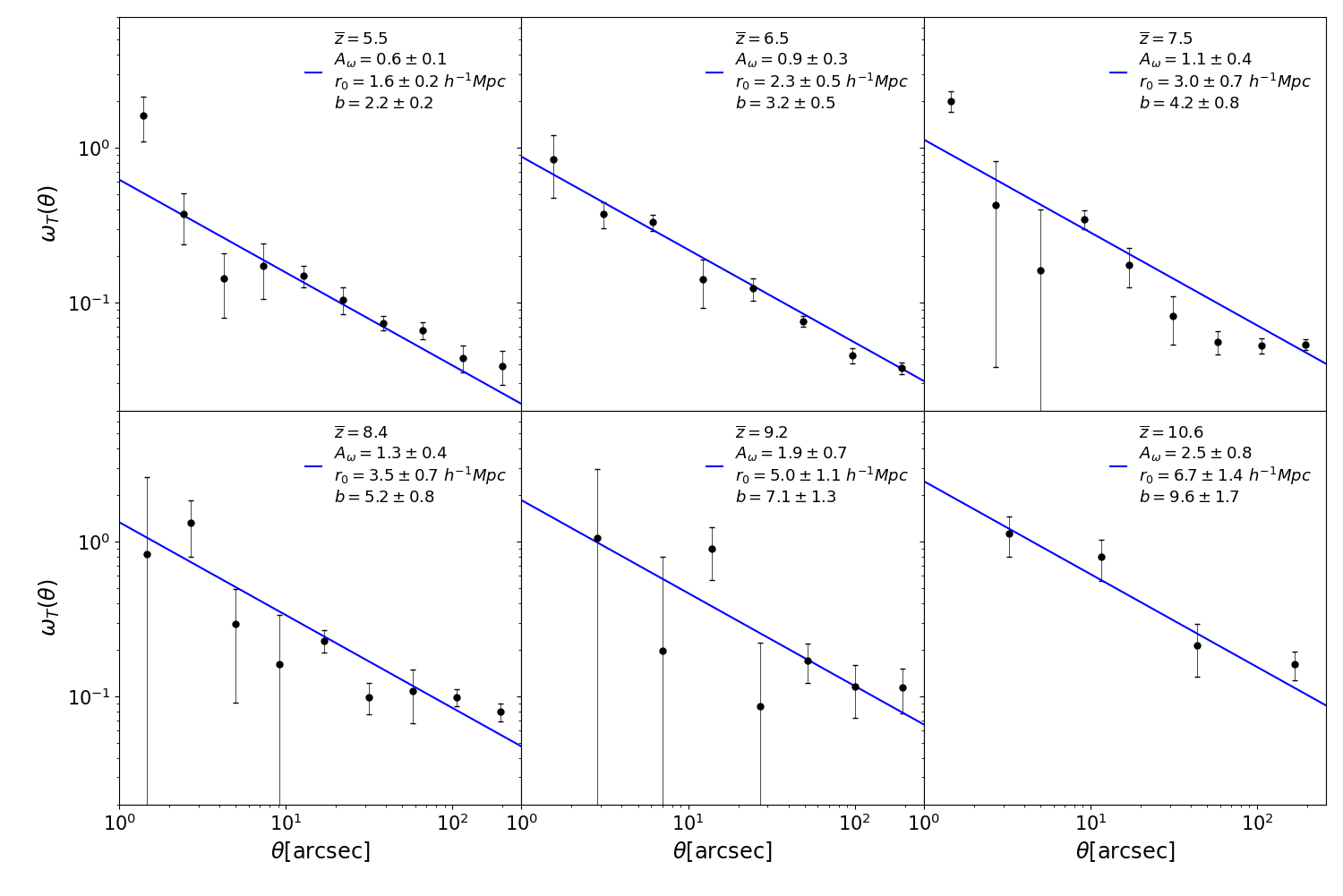
Figure 1: Measured ACFs in the GOODS-S field at six different mean redshifts. The objects in the sample have absolute magnitude $M_{F200W}<-15.5$. The black dots denote the ACF measurements with associated $1\sigma$ uncertainties, the blue solid lines represent a the power law best-fit with parameters listed in the legend box.

In Fig.2, the evolution of galaxy bias is presented, derived from the ACF shown in Fig.1 at six distinct redshifts. The dashed curves overlaying the plot correspond to the Sheth & Tormen (1999) bias of dark-matter halos at a fixed dark matter halo mass $M_{h}$. From the bias, we can also invert the relationship to obtain the characteristic dark matter halo mass hosting the observed galaxies. This is reported in column (8) of Tab.1. Fig. 2 also reports bias measurements in the literature, based primarily on Hubble Space Telescope and/or Subaru observations (Overzier et al. 2006; Barone-Nugent et al. 2014; Harikane et al. 2016; Qiu et al. 2018; Dalmasso et al. 2023). It should be noted that a direct comparison is not possible, as the JWST observations are substantially deeper. However, there is qualitative consistency since the bias we measure is lower than the previous measurements for brighter sources at fixed redshift. Intrinsically, our observations show a clear trend of increasing bias with redshift and a slight increase characteristic halo mass as well, which we interpret as a result of the evolution of the luminosity distance, which makes a magnitude limited survey probe brighter (and therefore more massive objects) at increasing redshift (e.g., Mason et al. 2015; Trenti et al. 2015).

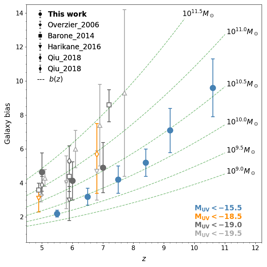
Figure 2: Galaxy bias evolution as a function of redshift $z$. Circles represent the results obtained in this work. Other symbols are previous bias measurements: stars Overzier et al. (2006), squares Barone-Nugent et al. (2014), downward triangles Harikane et al. (2016), diamonds Qiu et al. (2018) and upward triangles Dalmasso et al. (2023). Green dashed lines represent the theoretical bias evolution at a fixed dark matter halo mass $M_{h}$ $[M_{\odot}]$. Note that our observations are substantially deeeper than other studies, hence the inferred bias is lower.

4.2 Galaxy bias magnitude dependence

Interestingly, our sample is sufficiently large to explore luminosity dependence on galaxy bias by building subsamples of sources selected at different magnitude intervals for sources at redshifts $z\sim 5$, $z\sim 6$, and $z\sim 7$ (sources at higher redshift are too few to enable a split in magnitude subsamples). The magnitude bin size for each redshift selection has been chosen to ensure a balanced distribution of sources in each subsample, resulting in the average $M_{F200W}$ for each bin shown in Fig. 3. For comparison, we also report in this figure the results from prior studies on galaxy clustering. Reassuringly, with a consistent luminosity selection, our bias determination for the brightest samples are overlapping with prior measurements reported in the literature(Overzier et al. 2006; Barone-Nugent et al. 2014; Harikane et al. 2016; Qiu et al. 2018; Dalmasso et al. 2023). This agreement gives both confidence in our analysis, and also confirms that previous photometric samples of candidate galaxies at the end of the epoch of reionization have the same clustering properties as the higher quality JADES samples (which benefit from deeper data for improved photometric selection).

Fig.3 shows a decrease of bias with decreasing galaxy luminosity out to $M_{F200W}\sim-16$. This observed trend is effectively captured by the theoretical model for the bias evolution $b(M_{F200W})$ derived from Trenti et al. (2015) using the Gamma Ray Burst no-metal bias scenario, which traces star formation and therefore gives a halo mass- UV magnitude relationship we can plot against our data. Considering the simplicity of the model, it is remarkable that there is a good agreement with the observations.

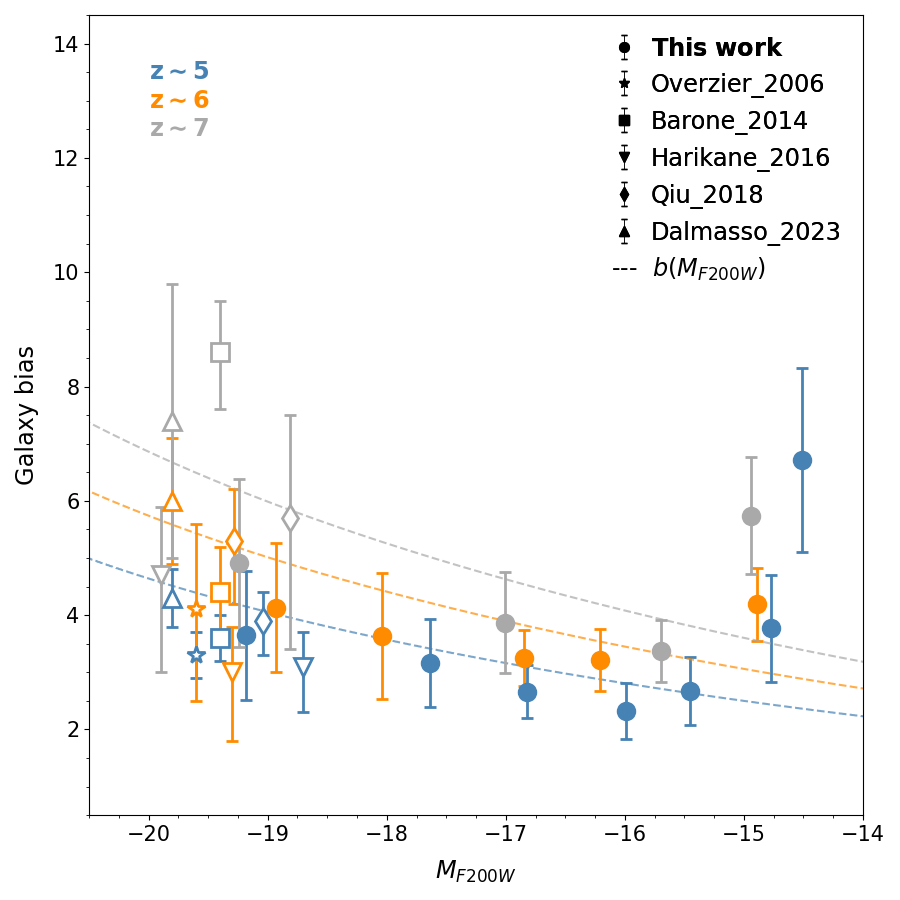
Figure 3: Galaxy bias evolution as a function of absolute magnitude $M_{F200W}$ for three different redshift bins (blue, orange and grey for $z=5,6,7$ respectively. Circles represent the results obtained in this work. Other symbols are literature measurements: stars Overzier et al. (2006), squares Barone-Nugent et al. (2014), downward triangles Harikane et al. (2016), diamonds Qiu et al. (2018) and upward triangles Dalmasso et al. (2023). Colored dashed lines represent the theoretical bias evolution model as a function of absolute magnitude $M_{F200W}$, derived from Trenti et al. (2015).

Interestingly, the initial decrease in bias as sources become fainter is reversed for the faintest objects in our sample, when our data probe a range of magnitudes that was inaccessible to previous observations. In fact, a distinct inflection point becomes apparent at $M_{F200W}\sim-15.0$, and the observed galaxy bias becomes significantly higher than the theoretical model that was providing a suitable data-model comparison for brighter (more massive) objects.
This change in the bias versus luminosity trend indicates a substantive shift in the underlying physics. We interpret this as a signature of the emergence of a one-halo term in the ACF once luminosities reach the typical values for dwarf galaxies. This means that the clustering signal at the faintest magnitudes we observe is carrying a significant contribution from halos hosting more than one galaxy. A full quantitative data-model comparison would require to build a Halo Occupation Distribution (HOD) model for fitting the observed ACF (e.g. Harikane et al. 2022). This is beyond the scope of this work and will be subject to future investations (which will also benefit from increased sample sizes and thus lower uncertainties). However, our ACF arguably carries such evidence already on closer inspection, particularly at lower redshifts. In fact, a noticeable deviation from a single power-law relationship for small angular separations ($\theta<10"$) can be seen in Fig.1.

4.3 Abundance matching and Duty Cycle

To explore the connection between dark mass and star formation at high redshift, we can resort to abundance matching and duty cycle modelling. This process entails statistically correlating the mass of dark matter halos with the luminosity (or stellar mass) of galaxies in a given sample. This methodology is based on the premise that the most luminous galaxy inhabits the most massive halo, followed by the second most massive galaxy residing in the subsequent most massive halo, and so forth. By doing so, it is possible to infer the intricate relationship between galaxy formation and the underlying dark matter structure (but see Ren et al. 2019). This relationship serves as the basis for calculating the duty cycle $\epsilon_{DC}$, which is defined as the fraction of time a dark matter halo of a certain mass hosts a UV-bright Lyman-Break Galaxies (LBGs) (e.g.,Martínez et al. 2002; Vale & Ostriker 2004). The fundamental equation forconducting abundance matching is:

$$\epsilon_{CD}\int_{M_{h}}^{+\infty}n(M_{h},z)dM_{h}=\int_{L_{g}}^{+\infty}\Phi(L,z)dL$$ (9)

Here, $\Phi(L,z)$ represents the Luminosity Function (LF) at redshift $z$, $n(M_{h},z)$ stands for the Dark Matter Halo Mass Function (MF) (Sheth & Tormen, 1999) and ($M_{h}$,$L_{g}$) are respectively the the minimum dark matter halo mass and the minimum luminosity of the galaxy. When it comes to the luminosity function parameters, we employed the parameters that exhibit evolution with redshift, as presented in Bouwens et al. (2021). The obtained duty cycle values are presented in the last column of Tab.1.
In our findings, we observe a growing trend linked to the redshift of the sample, peaking at a maximum duty cycle value of $\epsilon_{DC}=0.075^{+0.540}_{-0.067}$. This observation, observed at our highest redshift of $z=10.6$, aligns with the theoretical predictions outlined in Wyithe et al. 2014. The authors emphasized that for $z>4$, a low duty cycle ($\epsilon_{DC}\lesssim 0.15$) is necessary to reconcile the observed star formation rate with the relatively low observed total stellar mass. Within the redshift range examined in our study, we find duty cycle values below this theoretical threshold, confirming the existence of a previously unidentified population of UV-faint galaxies for $z>4$.

5 Summary and perspectives

In this paper, we utilised the methodology outlined and discussed in Dalmasso et al. (2023) to carry out galaxy clustering measurements well into the epoch of reionization (at redshift $z=10.6$) and for faint sources ($M_{F200W}\simeq-15.5$) using JWST data from the guaranteed time observation program JWST Advanced Deep Extragalactic Survey (JADES)(Bunker et al. 2023; Eisenstein et al. 2023; Hainline et al. 2023; Rieke et al. 2023) with the NIRCam instrument. Our main results and conclusions are as follows:
$\bullet$ We derived a galaxy bias measurement of $b=9.6\pm 1.7$ from a sample of $N_{g}=55$ candidates at redshift $z=10.6$.
$\bullet$ We studies self-consistently the clustering evolution from $5.0\leq z<10$. This allowed us to delineate the evolution of galaxy bias, revealing an increasing trend as anticipated by theory. Specifically, we report a value of $b=2.2\pm 0.2$ at $z=5.5$ and $b=7.1\pm 1.3$ at redshift $z=9.2$ (see Table 1).
$\bullet$ We uncovered a non-monotonic relationship between galaxy bias and magnitude (ig.3). While for bright sources there is a positive correlation with bias, the relationship has a minimum around $M_{F200W}\sim-15$, followed by a rapid rise of bias for the faintest sources. We interpret this behavior as evidence of the emergence of the one halo term in the clustering signal. This means that we are likely witnessing multiple sources hosted in the same dark matter halos (e.g. satellite galaxies).

Through this paper, we have demonstrated the viability of conducting clustering measurements on LBG samples observed during the epoch of reionization even as the candidates become increasingly faint and rare As photometric catalogs extend to even fainter magnitudes and the pool of available candidates expands from the growing number of JWST observations, the initial results reported here have the potential to blossom into a quantitative dataset to understand how early forming dark matter halos efficiently transform gas into stars.

Data Availability

The data used to conduct the analysis are from "The JWST Advanced Deep Extragalactic Survey (JADES)" (Bunker et al., 2023; Eisenstein et al., 2023; Hainline et al., 2023; Rieke et al., 2023).

References

- Ade et al. (2014) Ade P. A., et al., 2014, Astronomy & Astrophysics, 571, A16
- Adelberger et al. (2005) Adelberger K. L., Steidel C. C., Pettini M., Shapley A. E., Reddy N. A., Erb D. K., 2005, The Astrophysical Journal, 619, 697
- Akhlaghi & Ichikawa (2015) Akhlaghi M., Ichikawa T., 2015, The Astrophysical Journal Supplement Series, 220, 1
- AstropyCollaboration (2022) AstropyCollaboration 2022, The Astrophysical Journal, 935, 167
- Bahcall & Soneira (1980) Bahcall J. N., Soneira R. M., 1980, ApJS, 44, 73
- Bardeen et al. (1986) Bardeen J. M., Bond J. R., Kaiser N., Szalay A. S., 1986, ApJ, 304, 15
- Barone-Nugent et al. (2014) Barone-Nugent R. L., et al., 2014, The Astrophysical Journal, 793, 17
- Benoist et al. (1996) Benoist C., Maurogordato S., da Costa L. N., Cappi A., Schaeffer R., 1996, ApJ, 472, 452
- Bian et al. (2013) Bian F., et al., 2013, The Astrophysical Journal, 774, 28
- Bouwens et al. (2021) Bouwens R. J., et al., 2021, The Astronomical Journal, 162, 47
- Bradley et al. (2023) Bradley L., et al., 2023, astropy/photutils: 1.8.0, doi:10.5281/zenodo.7946442, https://doi.org/10.5281/zenodo.7946442
- Brammer et al. (2008) Brammer G. B., van Dokkum P. G., Coppi P., 2008, The Astrophysical Journal, 686, 1503
- Bullock et al. (2001) Bullock J. S., Kolatt T. S., Sigad Y., Somerville R. S., Kravtsov A. V., Klypin A. A., Primack J. R., Dekel A., 2001, MNRAS, 321, 559
- Bunker et al. (2023) Bunker A. J., et al., 2023, arXiv e-prints, p. arXiv:2306.02467
- Dalmasso et al. (2023) Dalmasso N., Trenti M., Leethochawalit N., 2023, Monthly Notices of the Royal Astronomical Society, p. stad3901
- Davis & Peebles (1983) Davis M., Peebles P. J. E., 1983, ApJ, 267, 465
- Eisenstein et al. (2023) Eisenstein D. J., et al., 2023, arXiv e-prints, p. arXiv:2306.02465
- Foucaud et al. (2003) Foucaud S., McCracken H. J., Le Fèvre O., Arnouts S., Brodwin M., Lilly S. J., Crampton D., Mellier Y., 2003, A&A, 409, 835
- Giavalisco & Dickinson (2001) Giavalisco M., Dickinson M., 2001, The Astrophysical Journal, 550, 177
- Hainline et al. (2023) Hainline K. N., et al., 2023, arXiv e-prints, p. arXiv:2306.02468
- Harikane et al. (2016) Harikane Y., et al., 2016, The Astrophysical Journal, 821, 123
- Harikane et al. (2022) Harikane Y., et al., 2022, The Astrophysical Journal Supplement Series, 259, 20
- Hatfield et al. (2018) Hatfield P. W., Bowler R. A. A., Jarvis M. J., Hale C. L., 2018, Monthly Notices of the Royal Astronomical Society, 477, 3760
- Jenkins et al. (2001) Jenkins A., Frenk C., White S. D., Colberg J. M., Cole S., Evrard A. E., Couchman H., Yoshida N., 2001, Monthly Notices of the Royal Astronomical Society, 321, 372
- Klypin et al. (1996) Klypin A., Primack J. R., Holtzman J. A., 1996, The Astrophysical Journal, 466, 13
- Landy & Szalay (1993) Landy S. D., Szalay A. S., 1993, ApJ, 412, 64
- Lee et al. (2006) Lee K., Giavalisco M., Gnedin O. Y., Somerville R. S., Ferguson H. C., Dickinson M., Ouchi M., 2006, The Astrophysical Journal, 642, 63
- Leethochawalit et al. (2022) Leethochawalit N., Trenti M., Morishita T., Roberts-Borsani G., Treu T., 2022, Monthly Notices of the Royal Astronomical Society, 509, 5836
- Ling et al. (1986) Ling E. N., Frenk C. S., Barrow J. D., 1986, Monthly Notices of the Royal Astronomical Society, 223, 21P
- Martínez et al. (2002) Martínez H. J., Zandivarez A., Merchán M. E., Domínguez M. J. L., 2002, MNRAS, 337, 1441
- Mason et al. (2015) Mason C. A., Trenti M., Treu T., 2015, The Astrophysical Journal, 813, 21
- Mo & White (1996) Mo H. J., White S. D. M., 1996, MNRAS, 282, 347
- Oke & Gunn (1983) Oke J. B., Gunn J. E., 1983, ApJ, 266, 713
- Okuta et al. (2017) Okuta R., Unno Y., Nishino D., Hido S., Loomis C., 2017, in Proceedings of Workshop on Machine Learning Systems (LearningSys) in The Thirty-first Annual Conference on Neural Information Processing Systems (NIPS). http://learningsys.org/nips17/assets/papers/paper_16.pdf
- Ouchi et al. (2004) Ouchi M., et al., 2004, The Astrophysical Journal, 611, 685
- Ouchi et al. (2005) Ouchi M., et al., 2005, The Astrophysical Journal, 635, L117
- Overzier et al. (2006) Overzier R. A., Bouwens R. J., Illingworth G. D., Franx M., 2006, The Astrophysical Journal, 648, l5
- Peacock & Nicholson (1991) Peacock J. A., Nicholson D., 1991, Monthly Notices of the Royal Astronomical Society, 253, 307
- Peebles (1980) Peebles P. J. E., 1980, The large-scale structure of the universe
- Persic & Salucci (1992) Persic M., Salucci P., 1992, MNRAS, 258, 14P
- Qiu et al. (2018) Qiu Y., et al., 2018, MNRAS, 481, 4885
- Ren et al. (2019) Ren K., Trenti M., Mason C. A., 2019, ApJ, 878, 114
- Rieke et al. (2023) Rieke M. J., et al., 2023, arXiv e-prints, p. arXiv:2306.02466
- Savoy et al. (2011) Savoy J., Sawicki M., Thompson D., Sato T., 2011, The Astrophysical Journal, 737, 92
- Sheth & Tormen (1999) Sheth R. K., Tormen G., 1999, Monthly Notices of the Royal Astronomical Society, 308, 119
- Tinker et al. (2010) Tinker J. L., Robertson B. E., Kravtsov A. V., Klypin A., Warren M. S., Yepes G., Gottlöber S., 2010, ApJ, 724, 878
- Trenti et al. (2010) Trenti M., Stiavelli M., Bouwens R. J., Oesch P., Shull J. M., Illingworth G. D., Bradley L. D., Carollo C. M., 2010, ApJ, 714, L202
- Trenti et al. (2015) Trenti M., Perna R., Jimenez R., 2015, ApJ, 802, 103
- Vale & Ostriker (2004) Vale A., Ostriker J. P., 2004, Monthly Notices of the Royal Astronomical Society, 353, 189
- Williams et al. (2018) Williams C. C., et al., 2018, ApJS, 236, 33
- Wyithe et al. (2014) Wyithe J. S. B., Loeb A., Oesch P. A., 2014, Monthly Notices of the Royal Astronomical Society, 439, 1326
- van der Walt et al. (2014) van der Walt S., et al., 2014, PeerJ, 2, e453