Online Time-Optimal Trajectory Generation for Two Quadrotors with Multi-Waypoints Constraints

Abstract

The autonomous quadrotor’s flying speed has kept increasing in the past $5$ years, especially in the field of autonomous drone racing. However, the majority of the research mainly focuses on the aggressive flight of a single quadrotor. In this letter, we propose a novel method called Pairwise Model Predictive Control (PMPC) that can guide two quadrotors online to fly through the waypoints with minimum time without collisions. The flight task is first modeled as a nonlinear optimization problem and then an efficient two-step mass point velocity search method is used to provide initial values and references to improve the solving efficiency so that the method can run online with a frequency of $50$ Hz and can handle dynamic waypoints. The simulation and real-world experiments validate the feasibility of the proposed method and in the real-world experiments, the two quadrotors can achieve a top speed of $8.1m/s$ in a $6$-waypoint racing track in a compact flying arena of $6m\times 4m\times 2m$.

Supplementary Material

Video : https://youtu.be/3jRnB1eAHEI.

I Introduction

In recent years, autonomous quadrotors have kept breaking the speed records and shown many potential applications such as emergency delivery services, search and rescue and rapid exploration in unknown and dangerous areas, etc. One of the driving forces behind these new records is autonomous drone racing, a platform for testing different elements of the drone’s autonomous agile flight, including navigation, trajectory generation and control techniques, etc. Since 2016, the speed of autonomous racing drones escalated from less than $1m/s$ to over $20m/s$ [1, 2, 3, 4, 5, 6]. One of the key technologies for achieving such a speed is the time-optimal trajectory generation methods and control techniques, which is a research hotspot focused by both academia and industry. However, the majority of the research on this topic mainly focuses on the aggressive flight of a single drone. As multi-drones with aggressive flight maneuvers can significantly improve the efficiencies of flying tasks and, in this work, we will focus on this problem and propose a method that can generate time-optimal trajectories for two quadrotors online to fly through the waypoints without collisions.

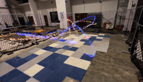
Figure 1: Two quadrotors race in a $6$-waypoint track and achieve a top speed of $8.1m/s$.

Many research achievements have been made on trajectory generation methods for single quadrotor’s high-speed flights. A classic aggressive trajectory generation method is the differential flatness and minimum-snap based method [7, 8] and subsequent improvements are made involving B-splines[9] and MINCO[10] to improve the computational efficiency and safety of the quadrotors. However, these trajectories cannot guarantee the time optimality due to their inherent smoothness. Another approach converts this trajectory generation problem into a nonlinear optimization problem and uses complementary progress variables (CPC) to force the quadrotor to pass waypoints in sequence [11]. While this method yields globally optimal trajectories, it often needs dozens of hours to solve the optimization problem. For online aggressive flight, the Model Predictive Contouring Control (MPCC) is a promising method that maximizes the progress along the reference trajectory and minimizes tracking errors, integrated with a mass point trajectory generation[12]. However, the complex sampling strategies fail to cope with rapidly changing dynamic waypoints. Recently, with the development of deep learning techniques, there has been work achieving high-speed agile flight through imitation learning[13, 14, 15] methods and reinforcement learning methods [16]. However, the former requires a pre-established large trajectory library which still cannot cover the quadrotors’ full state spaces, and the latter is only valid for specific tracks which limits its application in the real world.

For multi-quadrotors, swarms of quadrotors have been extensively studied for formation flight [17], search and rescue [18] and exploration tasks [19]. As time-optimality or aggressive flight is not the focus of these studies, the quadrotors don’t exhibit their inherent agile maneuverability. Game theory is also used in the autonomous drone racing of multi-quadrotors. However, the flight speed in the research is still far from the quadrotors’ boundaries [20, 21]. For high-speed multi-quadrotor flight tasks, existing work uses nonlinear optimization methods to generate optimal trajectories for multi-quadrotors [22, 23]. However, this method needs hours of offline computation and can only handle dynamic waypoints with prior known moving patterns but fails to handle waypoints online.

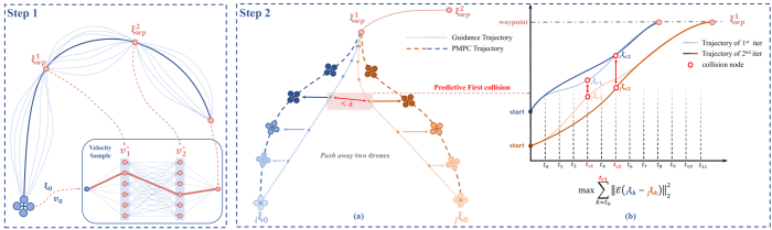
Figure 2: The pipeline of the proposed method. Step 1: A mass point is used to generate the global time-optimal trajectory which is used as the initial values and references for the optimization in Step 2. Step 2: An optimization problem is established to guide two quadrotors flying through the waypoints without collision.

Thus, in this letter, we propose a novel method of generating the time-optimal trajectories online for two quadrotors to pass through the waypoints in a pre-defined sequence (Fig. 2). The contributions of our study are outlined as follows:

1. A novel method called PMPC is developed to guide two quadrotors to fly through the pre-defined waypoints online with the minimum time.

2. An efficient two-step velocity search method to generate mass points’ global time-optimal trajectories is designed to serve as the initial values and references for the optimization problem.

3. The method is verified in both simulation and real-world experiments, where the quadrotors can achieve a top speed of $8.1m/s$ in a compact flight space.

II Time-Optimal Trajectory generation for Mass Points

Generating time-optimal trajectories online to pass through the waypoints is crucial for time-restrict flight tasks such as search and rescue or autonomous drone racing, etc. However, due to the nonlinearity of the quadrotor’s dynamics, it is difficult to effectively solve the optimization problem online. To solve this problem, we first simplify the quadrotor as a mass point and use this point mass model to analytically generate the time-optimal trajectories called mass point trajectory (Fig. 2. step 1). These trajectories will then serve as the initial values of the optimization problem with the full dynamics of the quadrotors and also the velocity reference for the quadrotors at the waypoints.

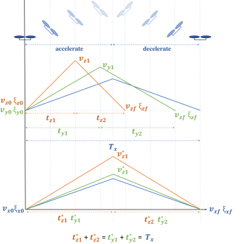
Figure 3: The travel time on each axis is different due to the different constraints. We use factor $\beta$ to equalize the travel time on each axis.

II-A Time-Optimal Trajectories between Two Points

For a one-dimension mass point, the solution of the time-optimal trajectories between two points is of bang-bang type [24]. The mass point will apply the maximum acceleration $a_{\max}$ from the start position $\xi_{0}$ and velocity $v_{0}$. After time $t_{1}$, at the switching point, where the position is $\xi_{1}$ and the velocity is $v_{1}$, it will apply the minimum acceleration $-a_{\max}$ until it reaches the target $\xi_{f}$ with the required velocity $v_{f}$ after time $t_{2}$. Given $\xi_{0}$, $v_{0}$, $\xi_{f}$, $v_{f}$ and $a_{\max}$, the switching point ($\xi_{1}$, $v_{1}$) and the flight time ($t_{1}$ and $t_{2}$) can be analytically calculated. As a result, the corresponding optimal trajectory can be obtained. We use $T=t_{1}+t_{2}$ to denote the time between the two points.

However, for a three-dimensional point-pass, different constraints on each axis, e.g. input constraints (${a_{z}}_{max}>{a_{x}}_{max}={a_{y}}_{max}$), initial constraints (${\xi_{x}}_{0}\neq{\xi_{y}}_{0}\neq{\xi_{z}}_{0}$) and target constraints (${\xi_{x}}_{f}\neq{\xi_{y}}_{f}\neq{\xi_{z}}_{f}$), lead to different travel time on each axis $T_{x}\neq T_{y}\neq T_{z}$. Thus, we use the acceleration reduction factor $\beta$ to reduce the acceleration on the axes with shorter travel time to equalize the travel time of each axis. For example, in Fig. 3, the travel time on $z$ axis $T_{z}$ and $y$ axis $T_{y}$ are shorter than $T_{x}$. We use $\beta_{z}$ to make the travel time on the $z$ axis equal to the travel time on the $x$ axis by solving

$${{\xi}_{z}}_{1} ={{\xi}_{z}}_{0}+{v_{z}}_{0}{t_{z}}_{1}^{*}+\frac{1}{2}\beta_{z}{a_{z}}_{\max}{{t_{z}}_{1}^{*}}^{2},$$ (1)

$${v_{z}}_{1} ={v_{z}}_{0}+\beta_{z}{a_{z}}_{\max}{{t_{z}}_{1}}^{*},$$

$${\xi_{z}}_{f} ={\xi_{z}}_{1}+{v_{z}}_{1}{t_{z}}_{2}^{*}-\frac{1}{2}\beta_{z}{a_{z}}_{\max}{t_{z}}_{2}^{*2},$$

$${v_{z}}_{f} ={v_{z}}_{1}-\beta_{z}{a_{z}}_{\max}{t_{z}}_{2}^{*},$$

where ${t_{z}}_{1}^{*}+{t_{z}}_{2}^{*}=T_{x}$. After solving (1), we can get $\beta_{z}$, ${t_{z}}_{1}^{*}$, ${\xi_{z}}_{1}$ and ${v_{z}}_{1}$. The result can be directly generalized to the $y$ axis.

II-B Two-step Time-Optimal Velocity Search

According to the last section, given the positions and the velocities of two waypoints, the optimal trajectory can be analytically calculated. Then how to determine the time-optimal velocity at the waypoints is another crucial factor for a multiple waypoint flight task. To solve this problem, we first construct a graph $\mathcal{G}=(\mathcal{V},\mathcal{E})$ as shown in Fig. 4 where the nodes $\mathcal{V}$ are the velocities at the waypoint and the edges $\mathcal{E}$ are the travel time between the waypoints. Among different combinations of the velocities at the waypoints, the one with the minimum travel time can be found by the Dijkstra method. With these velocities, the time-optimal trajectories of the mass point can be obtained.

To construct this graph, we first generate the nodes of the graph (the velocity at each waypoint) by sampling. One intuitive method is to randomly sample the velocities at the waypoints and with the increasing number of samples, the graph search converges to the optimal result. However, it is difficult to do a bulk sampling with the limited computing resources and online computing requirements. Thus, in this letter, we propose a two-step sampling method to efficiently sample the velocities and construct the graph.

As in the aggressive waypoint passing flight, the direction of the quadrotor’s velocity at the waypoint $i$ is approximately in parallel with the vector pointing from waypoint $i-1$ to waypoint $i$, which we denote by $\mathbf{v}_{i}$ (Fig. 4). However, the magnitudes of the velocities differ with the different relative positions of the next waypoint $i+1$. Thus, we first fix the direction of the velocities by $\mathbf{v}_{i}$ and sample the magnitude of the velocities.

$$\mathbf{v}_{i}=\frac{\boldsymbol{\xi}_{i}-\boldsymbol{\xi}_{i-1}}{\left\|\boldsymbol{\xi}_{i}-\boldsymbol{\xi}_{i-1}\right\|_{2}}.$$ (2)

By this method, we can prune a great amount of velocity candidates which are impossible to be the feasible velocities at the waypoints. For each waypoint, we generate $20$ velocity samples by

$$\mathcal{V}_{i}=\{1\times\mathbf{v}_{i},2\times\mathbf{v}_{i},...,20\times\mathbf{v}_{i}\}.$$ (3)

With the velocity samples at all the waypoints, we can calculate the edge $\mathcal{E}$ of the graph, the travel time between two adjacent waypoints, by the method described in the last section. In particular, the first node in graph $\mathcal{G}$ is the current quadrotor’s state. Then, the best velocities $v_{i}^{\rm min}$ at each waypoint can be found by the Dijkstra method.

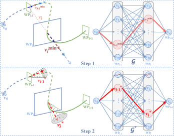
Figure 4: Step 1: sample velocities at the waypoints in the direction of $\mathbf{v}_{i}$ but in different magnitudes. Do a graph search to find the best velocities at the waypoints $v_{i}^{\rm min}$. Step 2: resample the velocities around $v_{i}^{\rm min}$ in different directions. Construct a new graph $\mathcal{G}^{*}$ with new samples and conduct the graph search again to find the optimal velocity $v_{i}^{*}$ at the $i^{th}$ waypoint.

However, as stated before, the above graph search is based on the assumption that the velocities at the waypoints are in parallel with $\mathbf{v}_{i}$, which is too strong. Thus, to further optimize the velocities at the waypoints, the second step is to regenerate velocity samples with the same magnitude with $v_{i}^{\min}$ but in different directions. All the velocity candidates at waypoint $i$ form a cone around $v_{i}^{\min}$ as shown in Fig. 4. Then a new graph $\mathcal{G}^{*}$ is constructed and we conduct the graph search again to find the optimal velocity $v_{i}^{*}$ at each waypoint. When the optimal velocities $v_{i}^{*}$ are determined, the time-optimal trajectories for the mass point passing through all the waypoints can be calculated analytically. This efficient two-step velocity search strategy and the analytical trajectory calculation make it possible for online planning for a point mass to handle dynamic environments and disturbances. However, there are differences between the mass point’s dynamics and the quadrotor’s dynamics, the optimal trajectories cannot guarantee the dynamic feasibility of the quadrotors. Thus, in the next section, we will introduce the optimization problem including the quadrotor’s full dynamics and use the mass point’s trajectories as initial values and references to establish the optimization problem and improve the solving efficiency.

III Trajectory Optimization Using Model Predictive Control

Although the strategy proposed in the last section can guide a point-mass passing through the waypoints with time optimality, it cannot guarantee dynamic feasibility and collision-free between quadrotors. To efficiently obtain time-optimal, dynamic feasible and collision-free trajectories for quadrotors, in this section, we establish a new optimization problem including the dynamics of two quadrotors to pass through all the waypoints. Additionally, we transform the hard constraints of collision avoidance into the optimization object to further increase the solving efficiency so that the optimization problem can be solved online with high frequency to form a model predictive control (MPC) strategy which we call Pairwise Model Predictive Control (PMPC). The quadrotors’ dynamics model we use is the same with [11]. For the reader’s convenience, we list the dynamics model here. It should be noted that we add the left subscript $j$ to the variables/states to denote that they belong to the $j^{th}$ quadrotor.

$$\prescript{}{j}{\dot{\mathbf{x}}}=\mathbf{f}_{dyn}(\prescript{}{j}{\mathbf{x}},\prescript{}{j}{\mathbf{u}})=\begin{cases}\prescript{}{j}{\mathbf{v}}\\ \mathbf{g}+\frac{1}{\prescript{}{j}{m}}\mathbf{R}(\prescript{}{j}{\mathbf{q}}){\prescript{}{j}{\mathbf{T}}}\\ \frac{1}{2}\Lambda(\prescript{}{j}{\mathbf{q}})\begin{bmatrix}0\\ \prescript{}{j}{\boldsymbol{\omega}}\end{bmatrix}\end{cases},$$ (4)

where

$${\prescript{}{j}{\mathbf{T}}}=\begin{bmatrix}0\\ 0\\ \sum\prescript{}{j}{{T}_{s}}\end{bmatrix}$$

is the thrust vector, $\prescript{}{j}{{T}_{s}}$ is the thrust of the rotors. In the equations above $\prescript{}{j}{\mathbf{v}}$, $\prescript{}{j}{\mathbf{q}}$ and $\prescript{}{j}{\boldsymbol{\omega}}$ are velocity, quaternions and angular velocity of the $j^{th}$ quadrotor, respectively. $\mathbf{R}(\prescript{}{j}{\mathbf{q}})$ is the rotation matrix. The inputs of the dynamic system in (4) is $\prescript{}{j}{\mathbf{u}}=[\sum\prescript{}{j}{T}_{s},\prescript{}{j}{\boldsymbol{\omega}}^{T}]^{T}$. The optimization target is

$$\mathcal{J}_{PMPC}=\prescript{}{1}{\mathcal{J}}_{wp}+\prescript{}{2}{\mathcal{J}}_{wp}-\mathcal{J}_{col},$$ (5)

where $\prescript{}{1}{\mathcal{J}}_{wp}$ and $\prescript{}{2}{\mathcal{J}}_{wp}$ are the terms for evaluating the quadrotors’ performance of approaching the waypoints while $\mathcal{J}_{col}$ is the term for collision avoidance which will be explained in the rest part of the section.

III-A Time-optimal Waypoint Approaching

Inspired by the observations of human pilot behavior that typically during the flight, the pilots consider only the next $2$ waypoints the quadrotors are approaching, we first set the optimization object as

$$\prescript{}{j}{\mathcal{J}}_{wp}=\sum_{k=0}^{N}\left\|\prescript{}{j}{\boldsymbol{\xi}}_{k}-{\boldsymbol{\xi}}_{wp}\right\|_{2}^{2}$$ (6)

to compel the quadrotor to arrive at the next waypoint as quickly as possible. In equation (6), $\prescript{}{j}{\boldsymbol{\xi}}_{k}$ is the $j^{th}$ quadrotor’s position at $k^{th}$ time step, and $\boldsymbol{\xi}_{wp}$ is the position of the next waypoint. $N$ is the number of steps in the prediction horizon. As the PMPC is required to run online, a long prediction horizon makes it difficult to solve the problem in real-time. Thus, in this work, the quadrotors predict only dozens of steps to improve the solving efficiency.

If we only consider arriving at the next waypoint as in equation (6), the quadrotor will fly towards it with the maximum effort which only guarantees the local optimality (minimum time towards the next waypoint) but loses the global optimality because the position of the following waypoint significantly affects the optimal trajectories. Thus, we add the mass point’s global optimal velocity $\mathbf{v}_{i}^{*}$ at the next waypoint $i$ (we use $\mathbf{v}_{wp}$ to substitute $\mathbf{v}_{i}^{*}$ in the following for the readers’ connivance) as another reference in the optimization object, which is a 3D vector but includes the information on how to approach the following waypoint so that the quadrotor not only considers how to arrive at the next waypoint as quickly as possible but also prepares for the following waypoint in advance. Then, the optimization object (6) becomes

$$\prescript{}{j}{\mathcal{J}}_{wp}=\sum_{k=0}^{N}\left\|\prescript{}{j}{\boldsymbol{\xi}}_{k}-{\boldsymbol{\xi}}_{wp}\right\|_{2}^{2}+\left\|\prescript{}{j}{\mathbf{v}}_{k}-{\mathbf{v}}_{wp}\right\|_{2}^{2}.$$ (7)

The two terms in equation (7) have different scales. Thus, two weighting parameters are needed to balance them. Moreover, the roles of the two terms differ during the waypoint approaching process. If we set fixed weights during the whole flight, the optimizer will find the ’best’ balance between the two terms. As a result, the quadrotor will neither pass through the waypoint nor achieve the desired velocities at the waypoints.

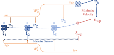
Figure 5: The dynamic weights are added to the optimization problem. When the quadrotors are far from the waypoint, they try their best to approach the waypoint with a higher $\mathcal{W}_{k}^{\xi}$. When the quadrotors are close to the waypoint, they need to have a velocity close to the mass point’s optimal velocity to prepare for passing through the following waypoint. Thus, they need higher $\mathcal{W}_{k}^{v}$

.

Thus, a dynamic weighting scheme should be employed to adjust the weights during the flight. When the quadrotor is far from the waypoint, we want it to approach the waypoint as fast as possible. Thus, the first term should have a larger weight. While the quadrotor is close to the waypoint, its velocity is expected to converge to the optimal velocity $\mathbf{v}_{wp}$ at the waypoint to prepare for passing through the following waypoint optimally. Thus, the weight of the second term should be increased. So, we develop sigmoid curves to generate the weights for the two terms in (7) during the flight (Fig. 5)

$$\prescript{}{j}{\mathcal{W}}_{k}^{\square}=\left\{\begin{aligned} \frac{1}{1+\text{exp}(-\sigma^{\xi}(\|\prescript{}{j}{\boldsymbol{\xi}}_{k}-\prescript{}{j}{\boldsymbol{\xi}}_{wp}\|_{2}^{2}-\mu)}&\\ \frac{1}{1+\text{exp}(-\sigma^{v}(\|\prescript{}{j}{\mathbf{v}}_{k}-\prescript{}{j}{\mathbf{v}}_{wp}\|_{2}^{2}-\mu)}&\\ \end{aligned}\right\}$$ (8)

where $\square=\{\xi,v\}$ and $\sigma^{\square}$ is the direction coefficient. $\mu$ is used to determine the time of weight change. These coefficients satisfy the following relationship:

$$\frac{\sigma^{\xi}}{\|\sigma^{\xi}\|}\frac{\sigma^{v}}{\|\sigma^{v}\|} =-1,$$

$$\sigma^{v} =10\sigma^{\xi}.$$

After adding dynamic weight factors $\prescript{}{j}{\mathcal{W}}_{k}^{\square}$ to equation (7), we have the optimization object as

$$\prescript{}{j}{\mathcal{J}}_{wp}=\sum_{k=0}^{N}\prescript{}{j}{\mathcal{W}}_{k}^{\xi}\left\|\prescript{}{j}{\boldsymbol{\xi}}_{k}-\prescript{}{j}{\boldsymbol{\xi}}_{wp}\right\|_{2}^{2}+\prescript{}{j}{\mathcal{W}}_{k}^{v}\left\|\prescript{}{j}{\mathbf{v}}_{k}-\prescript{}{j}{\mathbf{v}}_{wp}\right\|_{2}^{2}.$$ (9)

III-B Collision Avoidance between Two Quadrotors

The optimization object (9) mainly focuses on generating time-optimal trajectories for a single quadrotor. As the aim of this work is to develop a method of generating time-optimal trajectories for multi-quadrotors to pass through the waypoints, we need to add collision constraints to the optimization problem to ensure that the quadrotors do not collide with each other. We find that adding collision-free constraints

$$\left\|\mathbf{E}(\prescript{}{1}{\boldsymbol{\xi}_{k}}-\prescript{}{2}{\boldsymbol{\xi}}_{k})\right\|_{2}^{2}>\delta_{tol}\quad k\in[0,N],$$ (10)

where $\mathbf{E}$ is the matrix for relieving downwash risk [9], as hard constraints in the optimization problem as in [22] makes it difficult to solve the problem online or even fail to converge. Instead of modeling the collision-free constraints as the hard constraints, we put the constraints into the optimization object as soft constraints. Furthermore, to make the solving process easier, in our optimization problem, we only consider the collision-free constraints in part of the prediction horizon instead of the whole prediction horizon $N$. As shown in Fig. 2-(b) where the time-optimal trajectories of two mass points collide at time $t_{c,1}$ for the first time and then collide at $t_{c,2}$, in our optimization object, we only evaluate the distance between two quadrotors before the first collision by

$$\mathcal{J}_{col}=\sum_{k=t_{0}}^{t_{c}}\left\|\mathbf{E}(\prescript{}{1}{\boldsymbol{\xi}_{k}}-\prescript{}{2}{}{\boldsymbol{\xi}_{k}})\right\|_{2}^{2}$$ (11)

where $t_{c}=t_{c,1}$ is the time of the first collision between the two point mass’ trajectories. This term tries to divide two quadrotors’ trajectories from $t_{0}$ to $t_{c}$. It should be noted that this term can only guarantee that the two quadrotors do not collide before $t_{c}$. They still have a chance of collision after $t_{c}$. However, due to the high efficiency of the proposed method, the optimization problem can be solved online with high frequency ($50Hz$ in our case). Thus, during the flight, the optimization loop keeps running so that the quadrotors are always guaranteed to fly without collision in the upcoming time horizon.

III-C Optimization Problem Formulation

To conclude, the full PMPC can be expressed as

$$\underset{\mathbf{u}}{\min}\quad\mathcal{J}_{PMPC} =\prescript{}{1}{\mathcal{J}_{wp}}+\prescript{}{2}{\mathcal{J}_{wp}}-\mathcal{J}_{col}$$ (12)

subject to $$\mathbf{x}_{0}=\mathbf{x},$$

$$\mathbf{x}_{k+1}=f(\mathbf{x}_{k},\mathbf{u}_{k}),$$

$$\mathbf{u}_{\min}\leq\mathbf{u}\leq\mathbf{u}_{\max},$$

where $\mathbf{x}$ and $\mathbf{u}$ are vectors of the states and inputs of the two quadrotors. The first two terms ensure that the quadrotors can pass the pre-defined waypoints with the minimum time and the third term guarantees that they do not collide with each other in a short time horizon. The constraints ensure that the optimal trajectories start from the quadrotors’ current states and are dynamically feasible. With the optimal point mass trajectories as the initial value, this optimization problem can be solved online with high efficiency to form a nonlinear model predictive controller. During the flight, the PMPC can run online to control the quadrotors to fly through the waypoints with time optimality without collision with each other.

IV Simulation Results and Analysis

In this section, we design two simulation experiments to verify the effectiveness of the proposed method. The quadrotor model we use in the simulation is (4) and the numerical simulation is conducted by C++. The parameters used in the PMPC are listed in Table I.

TABLE I: The parameters used in simulation

parameters	value/range	parameters	value/range
$N$	$20$	$T_{s}[N]$	$[1,30]$
$\Delta t[s]$	$0.03$	$\omega_{x,y}[rad]$	$[-3,3]$
$\delta_{col}[m]$	$0.2$	$\mathbf{E}$	$diag(1,1,1/3)$
$\mu$	0.6	$\sigma^{\xi}$	10

The optimization problem (12) is solved using ACADO as the code generation tool and qpOASES as the solver. The prediction horizon size is set to $N=20$ while the timestep is set to $0.03s$. The solving time is about $20ms$ on a laptop with a CPU of Intel Core i9 running at $2.5$ GHz and RAM of 32G.

The first simulation experiment is designed to test the optimality of the proposed method. In this simulation, the PMPC drives a single quadrotor from a hover state at $[0,0,2]$ to another hover state $[10,0,2]$. At the same time, we use the CPC method as the benchmark to test the time optimality of the proposed method. The simulation result is shown in Fig. 6. It can be seen that both methods can drive the quadrotor to the target and have close arrival time where the PMPC’s arrival time is $1.85s$ and the CPC’s arrival time is $1.66s$, which indicates that the proposed method can achieve a near time-optimal performance. It should be noted that the PMPC can run online while the CPC method has to calculate the time-optimal trajectory offline using dozens of minutes or even hours.

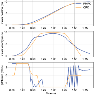
Figure 6: Comparison between the PMPC and CPC in a one-waypoint track.

The second simulation experiment is designed to simulate a drone racing track where two quadrotors start from hover states and pass through all the waypoints in a pre-defined sequence with the minimum time. The position of the waypoints is listed in Table II where the second waypoint is a moving waypoint used to test the online performance of the PMPC. In our previous work [22], we extend the CPC method to a swarm of quadrotors which we call the swarm-CPC. Thus, in this simulation, we use the swarm-CPC as the benchmark to demonstrate the performance of the proposed method. The result is shown in Fig. 7

TABLE II: The position of the waypoints

waypoint NO.	$1$	$2$	$3$	$4$	$5$	$6$
$x[m]$	$5$	$25$	$20$	$14$	$18$	$5$
$y[m]$	$15$	$5+y_{*}(t)$	$25$	$14$	$18$	$14$
$z[m]$	$2$	$3$	$5$	$2$	$6$	$4$

In this racing track, both methods can drive the two quadrotors to finish the track with their aggressive maneuverabilities without collision. The PMPC has a top speed of $20m/s$ and a lap time of $11.07s$ while the CPC has a top speed of $22m/s$ and a lap time of $10.6s$. Although the proposed method is slightly slower than the benchmark, it should be noted that the swarm-CPC requires hours of offline calculation and has to know the waypoints’ moving patterns in a prior while the proposed method can run online and only needs to know the waypoints’ current positions. The solving time of the PMPC and swarm-CPC is listed in Table III.

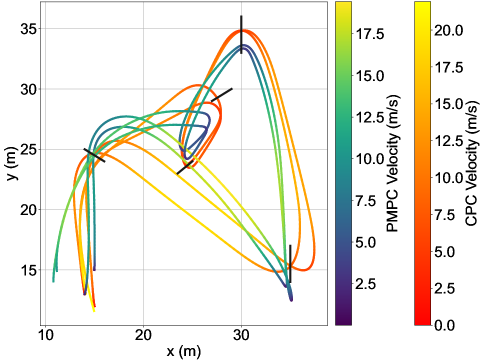
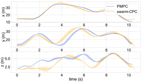
Figure 7: Trajectories of quadrotors with the PMPC and swarm-CPC. Although the PMPC is slightly slower than the swarm-CPC, it can achieve online performance.

TABLE III: Comparison with the benchmark

	solving time ($s$)	top speed ($m/s$)	flying time ($s$)
swarm-CPC	23.25 k	22	10.6
PMPC	0.02	20	11.07

V Real‐world Experiments

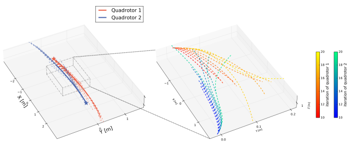
Figure 8: The trajectories of the quadrotors in the position-switching experiment. (left) The solid curves are the trajectories captured by the Optitrack system. The dashed curves are the optimization results of the PMPC at each step. (right) Partial enlarged drawing shows the predicted trajectories of the two quadrotors at each step.

We use two self-developed $100g$ quadrotors as our flying platforms. The onboard autopilot runs the Betaflight open-source software to provide low-level thrust and angular velocity control. The motion capture system, the Optitrack, is used to provide accurate position estimation. The PMPC runs on a laptop that communicates with the quadrotor using a lightweight WiFi module as shown in [15]. The experiment pipeline is shown in Fig.9. The flight space is a $6m\times 4m\times 2m$ free space as shown in Fig. 1.

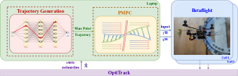
Figure 9: The system architecture. The PMPC is running on a laptop in real time. The angular velocity and throttle commands are fed to the quadrotors. The motion capture system, the OptiTrack, is used to provide accurate state estimation of the quadrotors.

We first design a simple position-switching experiment to demonstrate the feasibility of the proposed method in collision avoidance. In this experiment, two quadrotors first hover at $[-2,0,1]$ and $[2,0,1]$ respectively. The target position for them is the other’s starting point. The flight result can be found in Fig. 8 where the solid curves are the quadrotors’ trajectories captured by the OptiTrack system and the dashed curves optimization results of the PMPC at each step. We can find that the reference trajectories, which do not account for collision avoidance, are almost straight lines from the current position to the target, which accords with the time optimality. Then the PMPC split the two quadrotors while considering the quadrotors’ dynamics, collision-free constraints and also the time optimility. During the flight, the PMPC runs online with a frequency of $50$Hz. The minimum distance between the two quadrotors is $0.2m$ and the maximum speed achieves $5m/s$. It is also interesting to see that one quadrotor (blue) tends to have a straight trajectory, whereas the other quadrotor (red) undertakes more conflict avoidance tasks resulting in a more curved trajectory to minimize the total arrival time.

The second experiment (Fig. 1) is two quadrotors flying through a more complex racing track with $6$ waypoints. Fig. 10 shows the racing track and the trajectories of two quadrotors. In this experiment, two quadrotors start from their hover positions and pass through the same waypoints with a top speed of $8.1m/s$ without collision and finish the track within $6.31s$. From the experiments, we can see that the proposed method, the PMPC, performs well and can guide the quadrotors online to fly through the waypoints with their maximum maneuverability without collision.

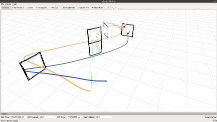
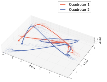
Figure 10: (a) The trajectories of the two quadrotors in the racing track. (b) The solid curves are the trajectories captured by the Optitrack. The dashed curves are the optimization result of the PMPC at each step.

VI Conclusion

In this letter, we present a novel method called PMPC for two autonomous drones to predict time-optimal trajectories online which pass through all the waypoints in a pre-defined sequence. The method first does a two-step optimal velocity search using a simple mass point model to provide global time-optimal trajectories as references. Then, based on the reference trajectories, an optimization problem is constructed to minimize the flight time with the quadrotors’ dynamics while keeping collision-free during the flight. Compared to the benchmark method, the PMPC is very computationally efficient so that it can be run online to handle the dynamic waypoints without the need for dozens of minutes or even hours to recalculate the optimal trajectories offline. The simulation and real-world experiments indicate that the proposed method can guide two quadrotors to fly through the waypoints without collision and achieve a very close arrival time compared to the benchmark method.

There are also several avenues for future investigation. For example, in this letter, the optimization is done on a laptop and the results are communicated with the quadrotors in real time. In the future, we will investigate moving all the computation onboard the quadrotors. Also, we will further study how to extend our work to more quadrotors so that it can be used for a swarm of quadrotors.

References

- [1] H. Moon, J. Martinez-Carranza, T. Cieslewski, M. Faessler, D. Falanga, A. Simovic, D. Scaramuzza, S. Li, M. Ozo, C. De Wagter, et al., “Challenges and implemented technologies used in autonomous drone racing,” Intelligent Service Robotics, pp. 1–12, 2019.
- [2] S. Li, M. M. Ozo, C. De Wagter, and G. C. de Croon, “Autonomous drone race: A computationally efficient vision-based navigation and control strategy,” Robotics and Autonomous Systems, vol. 133, p. 103621, 2020.
- [3] S. Li, E. van der Horst, P. Duernay, C. De Wagter, and G. C. de Croon, “Visual model-predictive localization for computationally efficient autonomous racing of a 72-g drone,” Journal of Field Robotics, vol. 37, no. 4, pp. 667–692, 2020.
- [4] C. De Wagter, F. Paredes-Vallés, N. Sheth, and G. de Croon, “The artificial intelligence behind the winning entry to the 2019 ai robotic racing competition,” arXiv preprint arXiv:2109.14985, 2021.
- [5] P. Foehn, A. Romero, and D. Scaramuzza, “Time-optimal planning for quadrotor waypoint flight,” Science Robotics, vol. 6, no. 56, p. eabh1221, 2021.
- [6] E. Kaufmann, L. Bauersfeld, A. Loquercio, M. Müller, V. Koltun, and D. Scaramuzza, “Champion-level drone racing using deep reinforcement learning,” Nature, vol. 620, no. 7976, pp. 982–987, 2023.
- [7] D. Mellinger and V. Kumar, “Minimum snap trajectory generation and control for quadrotors,” in 2011 IEEE International Conference on Robotics and Automation, pp. 2520–2525, IEEE, 2011.
- [8] M. Faessler, A. Franchi, and D. Scaramuzza, “Differential flatness of quadrotor dynamics subject to rotor drag for accurate tracking of high-speed trajectories,” IEEE Robotics and Automation Letters, vol. 3, no. 2, pp. 620–626, 2017.
- [9] X. Zhou, J. Zhu, H. Zhou, C. Xu, and F. Gao, “Ego-swarm: A fully autonomous and decentralized quadrotor swarm system in cluttered environments,” in 2021 IEEE international conference on robotics and automation (ICRA), pp. 4101–4107, IEEE, 2021.
- [10] Q. Wang, D. Wang, C. Xu, A. Gao, and F. Gao, “Polynomial-based online planning for autonomous drone racing in dynamic environments,” in 2023 IEEE/RSJ International Conference on Intelligent Robots and Systems (IROS), pp. 1078–1085, 2023.
- [11] P. Foehn, A. Romero, and D. Scaramuzza, “Time-optimal planning for quadrotor waypoint flight,” Science Robotics, vol. 6, no. 56, p. eabh1221, 2021.
- [12] A. Romero, S. Sun, P. Foehn, and D. Scaramuzza, “Model predictive contouring control for time-optimal quadrotor flight,” IEEE Transactions on Robotics, vol. 38, no. 6, pp. 3340–3356, 2022.
- [13] S. Li, E. Öztürk, C. De Wagter, G. C. De Croon, and D. Izzo, “Aggressive online control of a quadrotor via deep network representations of optimality principles,” in 2020 IEEE International Conference on Robotics and Automation (ICRA), pp. 6282–6287, IEEE, 2020.
- [14] R. Ferede, G. de Croon, C. De Wagter, and D. Izzo, “End-to-end neural network based optimal quadcopter control,” Robotics and Autonomous Systems, vol. 172, p. 104588, 2024.
- [15] J. Zhou, J. Mei, F. Zhao, J. Chen, and S. Li, “Imitation learning-based online time-optimal control with multiple-waypoint constraints for quadrotors,” arXiv e-prints, pp. arXiv–2402, 2024.
- [16] Y. Song, A. Romero, M. Müller, V. Koltun, and D. Scaramuzza, “Reaching the limit in autonomous racing: Optimal control versus reinforcement learning,” Science Robotics, vol. 8, no. 82, p. eadg1462, 2023.
- [17] L. Quan, L. Yin, T. Zhang, M. Wang, R. Wang, S. Zhong, X. Zhou, Y. Cao, C. Xu, and F. Gao, “Robust and efficient trajectory planning for formation flight in dense environments,” IEEE Transactions on Robotics, vol. 39, no. 6, pp. 4785–4804, 2023.
- [18] K. McGuire, C. De Wagter, K. Tuyls, H. Kappen, and G. C. de Croon, “Minimal navigation solution for a swarm of tiny flying robots to explore an unknown environment,” Science Robotics, vol. 4, no. 35, p. eaaw9710, 2019.
- [19] S.-J. Chung, A. A. Paranjape, P. Dames, S. Shen, and V. Kumar, “A survey on aerial swarm robotics,” IEEE Transactions on Robotics, vol. 34, no. 4, pp. 837–855, 2018.
- [20] R. Spica, E. Cristofalo, Z. Wang, E. Montijano, and M. Schwager, “A real-time game theoretic planner for autonomous two-player drone racing,” IEEE Transactions on Robotics, vol. 36, no. 5, pp. 1389–1403, 2020.
- [21] J. Di, S. Chen, P. Li, X. Wang, H. Ji, and Y. Kang, “A cooperative-competitive strategy for autonomous multidrone racing,” IEEE Transactions on Industrial Electronics, 2023.
- [22] Y. Shen, J. Zhou, D. Xu, F. Zhao, J. Xu, J. Chen, and S. Li, “Aggressive trajectory generation for a swarm of autonomous racing drones,” in 2023 IEEE/RSJ International Conference on Intelligent Robots and Systems (IROS), pp. 7436–7441, 2023.
- [23] Y. Shen, F. Zhao, J. Mei, J. Zhou, J. Xu, and S. Li, “Time-optimal trajectory generation with input boundaries and dynamic waypoints constraints for a swarm of quadrotors,” in 14th annual International Micro Air Vehicle Conference and Competition (D. Moormann, ed.), (Aachen, Germany), pp. 247–254, Sep 2023. Paper no. IMAV2023-31.
- [24] P. Foehn, D. Brescianini, E. Kaufmann, T. Cieslewski, M. Gehrig, M. Muglikar, and D. Scaramuzza, “Alphapilot: Autonomous drone racing,” Autonomous Robots, vol. 46, no. 1, pp. 307–320, 2022.