Diffusion Models as Constrained Samplers for Optimization
with Unknown Constraints

Abstract

Addressing real-world optimization problems becomes particularly challenging when analytic objective functions or constraints are unavailable. While numerous studies have addressed the issue of unknown objectives, limited research has focused on scenarios where feasibility constraints are not given explicitly. Overlooking these constraints can lead to spurious solutions that are unrealistic in practice. To deal with such unknown constraints, we propose to perform optimization within the data manifold using diffusion models. To constrain the optimization process to the data manifold, we reformulate the original optimization problem as a sampling problem from the product of the Boltzmann distribution defined by the objective function and the data distribution learned by the diffusion model. To enhance sampling efficiency, we propose a two-stage framework that begins with a guided diffusion process for warm-up, followed by a Langevin dynamics stage for further correction. Theoretical analysis shows that the initial stage results in a distribution focused on feasible solutions, thereby providing a better initialization for the later stage. Comprehensive experiments on a synthetic dataset, six real-world black-box optimization datasets, and a multi-objective optimization dataset show that our method achieves better or comparable performance with previous state-of-the-art baselines.

1 Introduction

Optimization problems are ubiquitous in real-world applications when approaching search problems (Bazaraa et al., 2011), partial differential equations (Isakov, 2006), molecular design (Sanchez-Lengeling & Aspuru-Guzik, 2018). While significant advancements have been made in resolving a broad spectrum of abstract optimization problems with analytically known objective functions and constraints  (Boyd & Vandenberghe, 2004; Rao, 2019; Petropoulos et al., 2023), optimization in real-world scenarios remains challenging since the exact nature of the objective is often unknown, and access to constraints is limited (Conn et al., 2009). For example, it is challenging to incorporate the closed-form constraints on a molecule to be synthesizable or design an objective function for target chemical properties.

Previous studies have identified problems with unknown objective functions as black-box optimization problems (Conn et al., 2009; Alarie et al., 2021). In such scenarios, the only way to obtain the objective value is through running a simulation (Larson et al., 2019) or conducting a real-world experiment (Shields et al., 2021), which might be expensive and non-differentiable. A prevalent approach to this challenge involves learning a surrogate model with available data to approximate the objective function which can be implemented in either an online (Snoek et al., 2012; Shahriari et al., 2015; Srinivas et al., 2010) or offline manner (Trabucco et al., 2021a, 2022).

However, there is a significant lack of research focused on scenarios where analytic constraints are absent. In practice, overlooking these feasibility constraints during optimization can result in spurious solutions. For instance, the optimization process might yield a molecule with the desired chemical property but cannot be physically synthesized (Gao & Coley, 2020; Du et al., 2022), which would require restarting the optimization from different initializations (Krenn et al., 2020; Jain et al., 2023).

To restrict the search space to the set of feasible solutions, we propose to perform optimization within the support of the data distribution or the data manifold. Indeed, in practice, one usually has an extensive set of samples satisfying the necessary constraints even when the constraints are not given explicitly. For instance, the set of synthesizable molecules can be described by the distribution of natural products (Baran, 2018; Voršilák et al., 2020). To learn the data distribution, we focus on using diffusion models, which recently demonstrated the state-of-the-art performance in image modeling (Ho et al., 2020; Song et al., 2020), video generation (Ho et al., 2022), and 3D synthesis (Poole et al., 2022). Moreover, Pidstrigach (2022); De Bortoli (2022) theoretically demonstrated that diffusion models can learn the data distributed on a lower dimensional manifold embedded in the representation space, which is often the case of the feasibility constraints.

To constrain the optimization process to the data manifold, we reformulate the original optimization problem as a sampling problem from the product of two densities: i) a Boltzmann density with energy defined by the objective function and ii) the density of the data distribution. The former concentrates around the global minimizers in the limit of zero temperature  (Hwang, 1980; Gelfand & Mitter, 1991), while the latter removes the non-feasible solutions by yielding the zero target density outside the data manifold. Note that one can easily extend the product of experts with more objective functions when multi-objective optimization is considered. Our optimization framework consists of two stages: (i) a guided diffusion process acts as a warm-up stage to provide initialization of data samples on the manifold, and (ii) we ensure convergence to the target distribution via Markov Chain Monte Carlo (MCMC). We also theoretically prove that the first stage yields a distribution that concentrates on the feasible minimizers in the zero temperature limit.

Empirically, we validate the effectiveness of our proposed framework on a synthetic toy example, six real-world offline black-box optimization tasks as well as a multi-objective molecule optimization task. We find that our method, named DiffOPT, can outperform state-of-the-art methods or achieve competitive performance across these tasks.

2 Background

Problem definition. Consider an optimization problem with objective function $h:\mathbb{R}^{d}\rightarrow\mathbb{R}$. Additionally, we consider a feasible set $C$, which is a subset of $\mathbb{R}^{d}$.

Our goal is to find the set of minimizers $\{x^{\star}_{i}\}_{i=1}^{M}$ of the objective $h$ within the feasible set $C$. This can be expressed as the following constrained optimization problem

$$\textstyle\{x^{\star}_{i}\}_{i=1}^{M}=\arg\min_{x\in C}h(x).$$

However, in our specific scenario, the explicit formulation of the feasible set $C$ is unavailable. Instead, we can access a set of points $\mathcal{D}=\{x_{i}\}_{i=1}^{N}$ sampled independently from the feasible set $C$.

Optimization via sampling. If we do not consider the constraints, under mild assumption, the optimization process is equivalent to sample from a Boltzmann distribution $q_{\beta}(x)\propto\exp[-\beta h(x)]$, in the limit where $\beta\to\infty$, where $\beta$ is an inverse temperature parameter. This is the result of the following proposition which can be found in Hwang (1980, Theorem 2.1).

Proposition 1.

Assume that $h\in\mathrm{C}^{3}(\mathbb{R}^{d},\mathbb{R})$. Assume that $\{x_{i}^{\star}\}_{i=1}^{M}$ is the set of minimizers of $h$. Let $p$ be a density on $\mathbb{R}^{d}$ such that there exists $i_{0}\in\{1,\dots,M\}$ with $p(x_{i_{0}}^{\star})>0$. Then $Q_{\beta}$ the distribution with density w.r.t the Lebesgue measure $\propto q_{\beta}(x)p(x)$ weakly converges to $Q_{\infty}$ as $\beta\to\infty$ and we have that

$$\textstyle Q_{\infty}=\sum_{i=1}^{M}a_{i}\updelta_{x_{i}^{\star}}/\sum_{i=1}^{M}a_{i},$$ (1)

with $a_{i}=p(x_{i}^{\star})\det(\nabla^{2}h(x_{i}^{\star}))^{-1/2}$.

Based on this proposition, (Gelfand & Mitter, 1991) proposed a tempered method for global optimization. However, the proposed temperature schedule scales logarithmically with the number of steps; hence, the total number of iterations scales exponentially, hindering this method’s straightforward application. In practice, we can sample from the density with the target high $\beta$, see (Raginsky et al., 2017; Ma et al., 2019; De Bortoli & Desolneux, 2021).

Product of Experts. To constrain our optimization procedure to the feasible set $C$, we propose to model the target density as a product of experts (Hinton, 2002), a modeling approach representing the “unanimous vote” of independent models. Given the density models of $m\in\mathbb{N}$ ”experts” $\{q_{i}(x)\}_{i=1}^{m}$, the target density of their product is defined as

$$\textstyle\pi(x)\propto\prod_{i=1}^{m}q_{i}(x)\,.$$ (2)

Hence, if one of the experts yields zero density at $x$, the total density of the product at $x$ is zero.

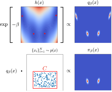
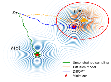
Figure 1: Constrained optimization as a sampling from the product of densities. That is, we minimize the objective function $h(x)$ (red stars denote the minimizers) within the feasible set $C$, which is given by samples $\{x_{i}\}_{i=1}^{N}\sim p(x)$. This problem is equivalent to sampling from the density $\pi_{\beta}(x)\propto p(x)\exp[-\beta h(x)]$, which concentrates around minimizers of $h(x)$ within the feasible set $C$. The distribution we sample from is shown on the left and the trajectory we take to sample is shown on the right.

Diffusion Models. Given a dataset $\mathcal{D}=\{x_{i}\}_{i=1}^{N}\sim p_{\text{data}}(x)^{\otimes N}$ with $p_{\text{data}}$ concentrated on the feasible set $C$, we will learn a generative model $p$ such that $p\approx p_{\text{data}}$ using a diffusion model (Sohl-Dickstein et al., 2015; Song & Ermon, 2019; Ho et al., 2020). The density $p$ will then be used in our product of experts model to enforce the feasibility constraints, see Section 3.1. In diffusion models, we first simulate a forward noising process starting from data distribution $p_{0}(x)=p_{\text{data}}(x)$ which converges to the standard Gaussian distribution $p_{T}(x)\approx\mathcal{N}(\textnormal{0},\mathrm{Id})$ as $T\rightarrow\infty$. The forward process is defined by the following stochastic differential equation (SDE)

$$\textnormal{d}\mathbf{x}^{{\mathchoice{\includegraphics[height=3.31529pt]{symbols/veryshortrightarrow.pdf}}{\includegraphics[height=3.31529pt]{symbols/veryshortrightarrow.pdf}}{\includegraphics[height=2.41112pt]{symbols/veryshortrightarrow.pdf}}{\includegraphics[height=1.50694pt]{symbols/veryshortrightarrow.pdf}}}}_{t}=f(\mathbf{x}^{{\mathchoice{\includegraphics[height=3.31529pt]{symbols/veryshortrightarrow.pdf}}{\includegraphics[height=3.31529pt]{symbols/veryshortrightarrow.pdf}}{\includegraphics[height=2.41112pt]{symbols/veryshortrightarrow.pdf}}{\includegraphics[height=1.50694pt]{symbols/veryshortrightarrow.pdf}}}}_{t},t)\textnormal{d}t+g(t)\textnormal{d}\mathbf{w}_{t},\;\mathbf{x}^{{\mathchoice{\includegraphics[height=3.31529pt]{symbols/veryshortrightarrow.pdf}}{\includegraphics[height=3.31529pt]{symbols/veryshortrightarrow.pdf}}{\includegraphics[height=2.41112pt]{symbols/veryshortrightarrow.pdf}}{\includegraphics[height=1.50694pt]{symbols/veryshortrightarrow.pdf}}}}_{0}\sim p_{\text{data}}(x),\;0\leq t\leq T\,,$$ (3)

where $f:\mathbb{R}^{d}\rightarrow\mathbb{R}^{d}$ is a vector-valued drift function, $g(t):\mathbb{R}\rightarrow\mathbb{R}$ is a scalar-valued diffusion coefficient, and $(\mathbf{w}_{t})_{t\geq 0}$ is a $d$-dimensional Brownian motion. Then, under mild assumptions, the reverse process that generates data from normal noise follows the backward SDE (Haussmann & Pardoux, 1986; Anderson, 1982)

$$\textnormal{d}\mathbf{x}^{{\mathchoice{\includegraphics[height=3.31529pt]{symbols/veryshortleftarrow.pdf}}{\includegraphics[height=3.31529pt]{symbols/veryshortleftarrow.pdf}}{\includegraphics[height=2.41112pt]{symbols/veryshortleftarrow.pdf}}{\includegraphics[height=1.50694pt]{symbols/veryshortleftarrow.pdf}}}}_{t}=\left[-f(\mathbf{x}^{{\mathchoice{\includegraphics[height=3.31529pt]{symbols/veryshortleftarrow.pdf}}{\includegraphics[height=3.31529pt]{symbols/veryshortleftarrow.pdf}}{\includegraphics[height=2.41112pt]{symbols/veryshortleftarrow.pdf}}{\includegraphics[height=1.50694pt]{symbols/veryshortleftarrow.pdf}}}}_{t},\tau)+g^{2}(\tau)\nabla_{x}\log p_{\tau}(\mathbf{x}^{{\mathchoice{\includegraphics[height=3.31529pt]{symbols/veryshortleftarrow.pdf}}{\includegraphics[height=3.31529pt]{symbols/veryshortleftarrow.pdf}}{\includegraphics[height=2.41112pt]{symbols/veryshortleftarrow.pdf}}{\includegraphics[height=1.50694pt]{symbols/veryshortleftarrow.pdf}}}}_{t})\right]\textnormal{d}t+g(\tau)\textnormal{d}\mathbf{w}_{t},\vspace{3mm}$$ (4)

where $\tau=T-t$ and $\nabla_{x}\log p_{\tau}(x)$ is the score function which is modeled by a time-dependent neural network via the score matching objective

$$\mathbb{E}_{t}\left[\lambda(t)\mathbb{E}_{\mathbf{x}_{0}^{\mathchoice{\includegraphics[height=2.36806pt]{symbols/veryshortrightarrow.pdf}}{\includegraphics[height=2.36806pt]{symbols/veryshortrightarrow.pdf}}{\includegraphics[height=1.72221pt]{symbols/veryshortrightarrow.pdf}}{\includegraphics[height=1.07639pt]{symbols/veryshortrightarrow.pdf}}}}\mathbb{E}_{\mathbf{x}_{t}^{\mathchoice{\includegraphics[height=2.36806pt]{symbols/veryshortrightarrow.pdf}}{\includegraphics[height=2.36806pt]{symbols/veryshortrightarrow.pdf}}{\includegraphics[height=1.72221pt]{symbols/veryshortrightarrow.pdf}}{\includegraphics[height=1.07639pt]{symbols/veryshortrightarrow.pdf}}}|\mathbf{x}_{0}^{\mathchoice{\includegraphics[height=2.36806pt]{symbols/veryshortrightarrow.pdf}}{\includegraphics[height=2.36806pt]{symbols/veryshortrightarrow.pdf}}{\includegraphics[height=1.72221pt]{symbols/veryshortrightarrow.pdf}}{\includegraphics[height=1.07639pt]{symbols/veryshortrightarrow.pdf}}}}\left[\|s_{\theta}(\mathbf{x}_{t}^{\mathchoice{\includegraphics[height=3.31529pt]{symbols/veryshortrightarrow.pdf}}{\includegraphics[height=3.31529pt]{symbols/veryshortrightarrow.pdf}}{\includegraphics[height=2.41112pt]{symbols/veryshortrightarrow.pdf}}{\includegraphics[height=1.50694pt]{symbols/veryshortrightarrow.pdf}}},t)-\nabla_{x}\log p_{t|0}(\mathbf{x}_{t}^{\mathchoice{\includegraphics[height=3.31529pt]{symbols/veryshortrightarrow.pdf}}{\includegraphics[height=3.31529pt]{symbols/veryshortrightarrow.pdf}}{\includegraphics[height=2.41112pt]{symbols/veryshortrightarrow.pdf}}{\includegraphics[height=1.50694pt]{symbols/veryshortrightarrow.pdf}}}|\mathbf{x}_{0}^{\mathchoice{\includegraphics[height=3.31529pt]{symbols/veryshortrightarrow.pdf}}{\includegraphics[height=3.31529pt]{symbols/veryshortrightarrow.pdf}}{\includegraphics[height=2.41112pt]{symbols/veryshortrightarrow.pdf}}{\includegraphics[height=1.50694pt]{symbols/veryshortrightarrow.pdf}}})\|^{2}_{2}\right]\right],\vspace{3mm}$$ (5)

where $p_{t|0}(\mathbf{x}_{t}^{\mathchoice{\includegraphics[height=3.31529pt]{symbols/veryshortrightarrow.pdf}}{\includegraphics[height=3.31529pt]{symbols/veryshortrightarrow.pdf}}{\includegraphics[height=2.41112pt]{symbols/veryshortrightarrow.pdf}}{\includegraphics[height=1.50694pt]{symbols/veryshortrightarrow.pdf}}}|\mathbf{x}_{0}^{\mathchoice{\includegraphics[height=3.31529pt]{symbols/veryshortrightarrow.pdf}}{\includegraphics[height=3.31529pt]{symbols/veryshortrightarrow.pdf}}{\includegraphics[height=2.41112pt]{symbols/veryshortrightarrow.pdf}}{\includegraphics[height=1.50694pt]{symbols/veryshortrightarrow.pdf}}})$ is the conditional density of the forward SDE starting at $\mathbf{x}_{0}^{\mathchoice{\includegraphics[height=3.31529pt]{symbols/veryshortrightarrow.pdf}}{\includegraphics[height=3.31529pt]{symbols/veryshortrightarrow.pdf}}{\includegraphics[height=2.41112pt]{symbols/veryshortrightarrow.pdf}}{\includegraphics[height=1.50694pt]{symbols/veryshortrightarrow.pdf}}}$, and $\lambda(t)>0$ is a weighting function. Under assumptions on $f$ and $g$, there exists $\alpha,\sigma$ such that for any $t\in[0,T]$, $\mathbf{x}_{t}^{\mathchoice{\includegraphics[height=3.31529pt]{symbols/veryshortrightarrow.pdf}}{\includegraphics[height=3.31529pt]{symbols/veryshortrightarrow.pdf}}{\includegraphics[height=2.41112pt]{symbols/veryshortrightarrow.pdf}}{\includegraphics[height=1.50694pt]{symbols/veryshortrightarrow.pdf}}}=\alpha_{t}\mathbf{x}_{0}^{\mathchoice{\includegraphics[height=3.31529pt]{symbols/veryshortrightarrow.pdf}}{\includegraphics[height=3.31529pt]{symbols/veryshortrightarrow.pdf}}{\includegraphics[height=2.41112pt]{symbols/veryshortrightarrow.pdf}}{\includegraphics[height=1.50694pt]{symbols/veryshortrightarrow.pdf}}}+\sigma_{t}\varepsilon$, where $\varepsilon\sim\mathcal{N}(0,\mathrm{Id})$, and therefore one does not need to integrate the forward SDE to sample $(\mathbf{x}_{0}^{\mathchoice{\includegraphics[height=3.31529pt]{symbols/veryshortrightarrow.pdf}}{\includegraphics[height=3.31529pt]{symbols/veryshortrightarrow.pdf}}{\includegraphics[height=2.41112pt]{symbols/veryshortrightarrow.pdf}}{\includegraphics[height=1.50694pt]{symbols/veryshortrightarrow.pdf}}},\mathbf{x}_{t}^{\mathchoice{\includegraphics[height=3.31529pt]{symbols/veryshortrightarrow.pdf}}{\includegraphics[height=3.31529pt]{symbols/veryshortrightarrow.pdf}}{\includegraphics[height=2.41112pt]{symbols/veryshortrightarrow.pdf}}{\includegraphics[height=1.50694pt]{symbols/veryshortrightarrow.pdf}}})$. Recent works have shown that diffusion models can detect the underlying data manifold supporting the data distribution (Pidstrigach, 2022; De Bortoli, 2022). This justifies the use of the output distribution of a diffusion model as a way to identify the feasible set.

3 Proposed Method

In this section, we present our method, DiffOPT. First, we formulate the optimization process as a sampling problem from the product of the data distribution concentrated on the manifold and the Boltzmann distribution defined by the objective function. Finally, we propose a two-stage sampling framework with different design choices.

3.1 Constrained Optimization as Sampling from Product of Experts

We recall that $q_{\beta}(x)\propto\exp[-\beta h(x)]$, where $h$ is the objective function. While it is possible to sample directly from $q_{\beta}(x)$, the generated samples may fall outside of the feasible set $C$, defined by the dataset $\mathcal{D}$. To address this, we opt to sample from the product of the data distribution and the Bolzmann distribution induced by the objective function. Explicitly, our goal is to sample from a distribution $\pi_{\beta}(x)$ defined as

$$\textstyle\pi_{\beta}(x)\propto p(x)q_{\beta}(x).$$ (6)

Using Proposition 1, we have that $\pi_{\beta}$ concentrates on the feasible minimizers of $h$ as $\beta\to+\infty$.

It should be noted that Equation 6 satisfies the following properties: (a) it assigns high likelihoods to points $x$ that simultaneously exhibit sufficiently high likelihoods under both the base distributions $p(x)$ and $q_{\beta}(x)$; (b) it assigns low likelihoods to points $x$ that display close-to-zero likelihood under either one or both of these base distributions. This approach ensures that the generated samples not only remain within the confines of the data manifold but also achieve low objective values.

Extending our framework to the multi-objective optimization setting is straightforward. Suppose we aim to maximize a set of objectives, denoted as $\{h^{1},h^{2},\ldots\}$. In this context, the optimization process can be represented by the distribution $\pi(x)$, which is proportional to the product of the data distribution and the individual Boltzmann distributions for each objective, expressed as $\pi(x)\propto p(x)\prod_{i}q^{i}_{\beta}(x)$.

3.2 DiffOPT: Two-stage Sampling with Optimization-guided Diffusion

Under mild assumptions on $\pi_{\beta}$, the following SDE converges to $\pi_{\beta}$ w.r.t.  the total variation distance (Roberts & Tweedie, 1996)

$$\textnormal{d}\mathbf{x}_{t}=\nabla_{\mathbf{x}}\log\pi_{\beta}(\mathbf{x}_{t})\textnormal{d}t+\sqrt{2}\textnormal{d}\mathbf{w}_{t}.$$ (7)

where the gradient of the unnormalized log-density can be conveniently expressed as the sum of the scores, i.e.,  $\nabla_{x}\log\pi_{\beta}(x)=\nabla_{x}\log p(x)+\nabla_{x}\log q_{\beta}(x)$. Furthermore, one can introduce a Metropolis-Hastings (MH) correction step to guarantee convergence to the target distribution when using discretized version of Equation 7 (Durmus & Moulines, 2022), which is known as the Metropolis-Adjusted-Langevin-Algorithm (MALA) (Grenander & Miller, 1994). We provide more details and the pseudocode for both algorithms in Appendix A.

Theoretically, sampling from the density in Equation 6 can be done via MALA. However, in practice, the efficiency of this algorithm significantly depends on the choice of the initial distribution and the step size schedule. The latter is heavily linked with the Lipschitz constant of $\log q_{\beta}$ which controls the stability of the algorithm. Large values of $\beta$, necessary to get accurate minimizers, also yield large Lipschitz constants which in turn impose small stepsizes. Moreover, the gradient of the log-density can be undefined outside the feasibility set $C$.

To circumvent these practical issues, we propose sampling in two stages: a warm-up stage and a sampling stage. The former aims to provide a good initialization for the sampling stage. The sampling stage follows the Langevin dynamics for further correction. The pseudocode for both stages is provided in Algorithm 1.

Stage I: Warm-up with guided diffusion. In imaging inverse problems, it is customary to consider guided diffusion models to enforce some external condition, see (Chung et al., 2022a, b; Song et al., 2022; Wu et al., 2023). In our setting, we adopt a similar strategy where the guidance term is given by $\beta h$, i.e., we consider

$$\textnormal{d}\mathbf{x}^{{\mathchoice{\includegraphics[height=3.31529pt]{symbols/veryshortleftarrow.pdf}}{\includegraphics[height=3.31529pt]{symbols/veryshortleftarrow.pdf}}{\includegraphics[height=2.41112pt]{symbols/veryshortleftarrow.pdf}}{\includegraphics[height=1.50694pt]{symbols/veryshortleftarrow.pdf}}}}_{t}=[ -f(\mathbf{x}^{{\mathchoice{\includegraphics[height=3.31529pt]{symbols/veryshortleftarrow.pdf}}{\includegraphics[height=3.31529pt]{symbols/veryshortleftarrow.pdf}}{\includegraphics[height=2.41112pt]{symbols/veryshortleftarrow.pdf}}{\includegraphics[height=1.50694pt]{symbols/veryshortleftarrow.pdf}}}}_{t},\tau)+g^{2}(\tau)s_{\theta}(\mathbf{x}^{{\mathchoice{\includegraphics[height=3.31529pt]{symbols/veryshortleftarrow.pdf}}{\includegraphics[height=3.31529pt]{symbols/veryshortleftarrow.pdf}}{\includegraphics[height=2.41112pt]{symbols/veryshortleftarrow.pdf}}{\includegraphics[height=1.50694pt]{symbols/veryshortleftarrow.pdf}}}}_{t},\tau)$$ (8)

$$-\beta\nabla h({\mathbf{x}}_{t}^{\mathchoice{\includegraphics[height=3.31529pt]{symbols/veryshortleftarrow.pdf}}{\includegraphics[height=3.31529pt]{symbols/veryshortleftarrow.pdf}}{\includegraphics[height=2.41112pt]{symbols/veryshortleftarrow.pdf}}{\includegraphics[height=1.50694pt]{symbols/veryshortleftarrow.pdf}}})]\textnormal{d}t+g(\tau)\textnormal{d}\mathbf{w}_{t},\quad\tau=T-t.$$ (9)

It is known that guided diffusion does not sample from the product of experts $q_{\beta}$ (Du et al., 2023b; Garipov et al., 2023). While Sequential Monte Carlo corrections have been proposed to correct this behavior (Cardoso et al., 2023; Wu et al., 2023), in this work, we do not consider such correction but instead show that for large value of $\beta$ the output distribution of the guided process concentrates on the feasible minimizers. We obtain the following result by combining the properties of diffusion models and the Feynamn-Kac theorem.

Theorem 1.

Under assumptions on $p$, $h$ and assuming that $\beta$ is replaced by $\beta(\tau)$ and $\beta(t)=1/t$ if $t>1/\beta_{0}$ and $0$ otherwise, we denote $p_{T-t}^{\beta}$ the distribution of Equation 8 at time $t$ and there exists $C>0$ such that for any $x\in\mathbb{R}^{d}$

$$(1/C)\tilde{p}_{0}^{\beta}(x)\leq p_{0}^{\beta}(x)\leq C\tilde{p}_{0}^{\beta}(x),$$ (10)

where $p_{0}^{\beta}$ is the output of the warm-up guided diffusion process and

$$\tilde{p}_{0}^{\beta}(x)=p_{0}(x)\exp[\log(\beta_{0})W_{0}^{\beta}(x)],$$ (11)

with $W_{0}^{\beta}(x)=\Delta h(x)+\langle\nabla\log p_{0}^{\beta}(x),\nabla h(x)\rangle$.

The proof is postponed to Appendix C. In Theorem 1, we show that the output distribution of the warm-up process is upper and lower bounded by a product of experts comprised of (i) $p_{0}$which ensures the feasibility conditions (ii) $\exp[\log(\beta_{0})W_{0}^{\beta}]$related to the optimization of the objective. As an immediate consequence of Theorem 1, we have that $\lim_{\beta_{0}\to\infty}p_{0}^{\beta}(x_{\star})=+\infty$ for every local strict minimizer $x^{\star}$ of $h$ within the support of $p_{0}(x)$, and $\lim_{\beta_{0}\to\infty}p_{0}^{\beta}(x_{\star})=0$ for $x^{\star}$ outside the support of $p_{0}(x)$, see Appendix C. That is, $p_{0}^{\beta}$ concentrates on the feasible local minimizers of $h$ as $\beta_{0}\to+\infty$.

Algorithm 1 Sampling via DiffOPT

0:  inverse temperature schedule $\beta(t)$, diffusion volatility schedule $g(t)$ and drift $f(x,t)$, score model $s_{\theta}(x_{t},t)$, energy function of the data distribution $E_{\theta}(x,t)$ if applying the MH correction.

1:  $\mathcal{X}\leftarrow\varnothing$

2:  Sample $x_{0}\sim\mathcal{N}(0,\mathrm{Id})$

3:  // Stage I: Warm-up with guided diffusion.

4:  for $t=0,\ldots,T$ do

5:     Draw $z\sim\mathcal{N}(0,\mathrm{Id})$, define $\tau=T-t$

6:     $x_{t+\Delta t}\leftarrow x_{t}+[-f(x_{t},\tau)+g^{2}(\tau)s_{\theta}(x_{t},\tau)$

7:     $\qquad\qquad\qquad\;-\beta(\tau)\nabla_{x_{t}}h(x_{t})]\Delta t+g(\tau)\sqrt{\Delta t}z$

8:  end for

9:  // Stage II: Further correction with Langevin dynamics.

10:  for $t=T,\ldots,T^{\prime}$ do

11:     Draw $z\sim\mathcal{N}(0,\mathrm{Id})$

12:     $\hat{x}\leftarrow x+[s_{\theta}(x,0)-\beta\nabla h(x)]\Delta t+\sqrt{2\Delta t}z$

13:     if applying Metropolis-Hastings test then

14:        $u\sim\text{Uniform}[0,1]$

15:        $\ell_{\theta}(\hat{x})=E_{\theta}(\hat{x},0)-\beta h(\hat{x})$

16:        $\ell_{\theta}(x)=E_{\theta}(x,0)-\beta h(x)$

17:        $\ell(\hat{x},x)=-\|x-\hat{x}-\Delta t[s_{\theta}(\hat{x},0)-\beta\nabla h(\hat{x})]\|^{2}$

18:        $\ell(x,\hat{x})=-\|\hat{x}-x-\Delta t[s_{\theta}(x,0)-\beta\nabla h(x)]\|^{2}$

19:        $\ell_{\text{acc}}=\ell_{\theta}(\hat{x})-\ell_{\theta}(x)+(\ell(\hat{x},x)-\ell(x,\hat{x}))/(2\Delta t)$

20:        $\text{if }\;\;\ell_{\text{acc}}>\log(u),\;\;\text{ then }\;\;x\leftarrow\hat{x}$

21:     else

22:        $x\leftarrow\hat{x}$

23:     end if

24:     $\mathcal{X}\leftarrow\mathcal{X}\cup\{x\}$

25:  end for

25:  $\mathcal{X}$

Stage II: Further correction with Langevin dynamics. The guided diffusion process in the first stage yields a more effectively initialized distribution within the data manifold, bounded both above and below by a product of experts related to the original constrained optimization problem. In the second stage, we further use Langevin dynamics for accurate sampling from $\pi_{\beta}(x)$. The gradient of the log-density of the data distribution $\nabla\log p(x)$ can be obtained by setting the time of the score function to 0, i.e., $s_{\theta}(x,0)$. The unadjusted Langevin algorithm is then given by

$$\textstyle x^{k+1}=x^{k}+(s_{\theta}(x^{k},0)-\beta\nabla_{x}h(x^{k}))\Delta t+\sqrt{2\Delta t}z,$$ (12)

where $\Delta t$ is the step size and $z$ comes from a Gaussian distribution. In practice, we find that a constant $\beta$ is enough for this stage. When using the score-based parameterization $s_{\theta}(x,t)$, we cannot access the unnormalized log-density of the distribution. Therefore, we cannot use the MH correction step. Although the sampler is not exact without MH correction, it performs well in practice.

To further incorporate the MH correction step, we can adopt an energy-based parameterization following Du et al. (2023b): $E_{\theta}(x,t)=-\frac{1}{2}\|\text{NN}_{\theta}(x,t)\|^{2}$, where $E_{\theta}(x,t)$ is the energy function of the data distribution, and $\text{NN}_{\theta}(x,t)$ is a vector-output neural network. An additional benefit of MH correction is one can automatically tune the hyperparameters, such as the step size according to the acceptance rate (Du et al., 2023b). We provide more details of this energy-based parameterization in Appendix B.

Extension to black-box objective. Our framework can be easily adapted to black-box optimization. In such a case, we utilize a logged dataset, denoted as $\{x_{i},y_{i}\}_{i=1}^{N}$, where each $y_{i}$ represents the objective value evaluated at the point $x_{i}$. This dataset allows us to train a surrogate objective function $h_{\phi}(x)$ using deep neural networks.

4 Related Work

Diffusion models and data manifold. Diffusion models have demonstrated impressive performance in various generative modeling tasks, such as image generation (Song et al., 2020; Ho et al., 2020), video generation (Ho et al., 2022), and protein synthesis (Watson et al., 2023; Gruver et al., 2023). Several studies reveal diffusion models implicitly learn the data manifold (Pidstrigach, 2022; De Bortoli et al., 2021; Du et al., 2023a; Wenliang & Moran, 2023). This feature of diffusion models has been used to estimate the intrinsic dimension of the data manifold in (Stanczuk et al., 2022). Moreover, the concentration of the samples on a manifold can be observed through the singularity of the score function. This phenomenon is well-understood from a theoretical point of view and has been acknowledged in (De Bortoli, 2022; Chen et al., 2022).

Optimization as sampling problems. Numerous studies have investigated the relationship between optimization and sampling (Ma et al., 2019; Stephan et al., 2017; Trillos et al., 2023; Wibisono, 2018; Cheng, 2020; Cheng et al., 2020). Sampling-based methods have been successfully applied in various applications of stochastic optimization when the solution space is too large to search exhaustively (Laporte et al., 1992) or when the objective function exhibits noise (Branke & Schmidt, 2004) or countless local optima (Burke et al., 2005, 2020). A prominent solution to global optimization is through sampling with Langevin dynamics (Gelfand & Mitter, 1991), which simulates the evolution of particles driven by a potential energy function. Furthermore, simulated annealing (Kirkpatrick et al., 1983) employs local thermal fluctuations enforced by Metropolis-Hastings updates to escape local minima (Metropolis et al., 1953; Hastings, 1970). More recently, Zhang et al. (2023) employs GFlowNet to amortize the cost of the MCMC sampling process for combinatorial optimization with both closed-form objective function and constraint.

Learning for optimization. Recently, there has been a growing trend of adopting machine learning methods for optimization tasks. The first branch of work is model-based optimization, which focuses on learning a surrogate model for the black-box objective function. This model can be developed in either an online (Snoek et al., 2012; Shahriari et al., 2015; Srinivas et al., 2010; Zhang et al., 2021), or an offline manner (Yu et al., 2021; Trabucco et al., 2021b; Fu & Levine, 2020; Chen et al., 2023; Yuan et al., 2023). Additionally, some research (Kumar & Levine, 2020; Krishnamoorthy et al., 2023; Kim et al., 2023) has explored the learning of stochastic inverse mappings from function values to the input domain, utilizing generative models such as Generative Adversarial Nets (Goodfellow et al., 2014) and Diffusion Models (Song et al., 2020; Ho et al., 2020).

The second branch, known as “Learning to Optimize, ” involves training a deep neural network to address specific optimization problems. In these works, the model is trained using a variety of instances within this problem category, to achieve generalization to novel, unseen instances. Various learning paradigms have been used in this context, including supervised learning (Li et al., 2018; Gasse et al., 2019), reinforcement learning (Li & Malik, 2016; Khalil et al., 2017; Kool et al., 2018), unsupervised learning (Karalias & Loukas, 2020; Wang et al., 2022; Min et al., 2023), and generative modeling (Sun & Yang, 2023; Li et al., 2023). In contrast to our approach, these works typically involve explicitly defined objective functions and constraints.

5 Experiment

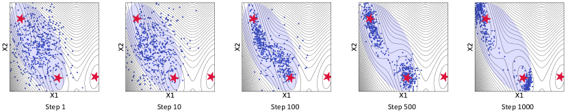
Figure 2: Sampling trajectory of DiffOPT in the synthetic Branin experiment with unknown constraints. Red stars denote the minimizes, and the blue region denotes the feasible space from which training data is sampled. DiffOPT can effectively navigate towards the two feasible minimizers.

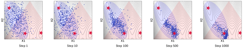
Figure 3: Sampling trajectory of DiffOPT in the synthetic Branin experiment with additional known constraints. Red stars denote the minimizers, the blue region denotes the feasible space from which training data is sampled and the pink region denotes the feasible space defined by the added given constraints. DiffOPT can effectively navigate towards the unique minimizer at the intersection of the two feasible spaces.

Baseline	TFBind8	TFBind10	Superconductor	Ant	D’Kitty	ChEMBL	Mean Rank
Dataset Best	$0.439$	$0.00532$	$74.0$	$165.326$	$199.231$	$383.7e3$	-
CbAS	$0.958$$\pm$0.018	$0.761$$\pm$0.067	$83.178$$\pm$15.372	$468.711$$\pm$14.593	$213.917$$\pm$19.863	$389.0e3$$\pm$0.5e3	$6.33$
GP-qEI	$0.824$$\pm$0.086	$0.675$$\pm$0.043	$92.686$$\pm$3.944	$480.049$$\pm$0.000	$213.816$$\pm$0.000	$388.1e3$$\pm$0.0	$7.17$
CMA-ES	$0.933$$\pm$0.035	$0.848$$\pm$0.136	$90.821$$\pm$0.661	$\mathbf{1016.409}$$\pm$906.407	$4.700$$\pm$2.230	$388.4e3$$\pm$0.4e3	$5.17$
Gradient Ascent	$\underline{0.981}$$\pm$0.010	$0.770$$\pm$0.154	$93.252$$\pm$0.886	$-54.955$$\pm$33.482	$226.491$$\pm$21.120	$390.1e3$$\pm$2.0e3	$4.33$
REINFORCE	$0.959$$\pm$0.013	$0.692$$\pm$0.113	$89.469$$\pm$3.093	$-131.907$$\pm$41.003	$-301.866$$\pm$246.284	$388.4e3$$\pm$2.1e3	$7.33$
MINs	$0.938$$\pm$0.047	$0.770$$\pm$0.177	$89.027$$\pm$3.093	$533.636$$\pm$17.938	$\underline{272.675}$$\pm$11.069	$\underline{391.0e3}$$\pm$0.2e3	$4.50$
COMs	$0.964$$\pm$0.020	$0.750$$\pm$0.078	$78.178$$\pm$6.179	$540.603$$\pm$20.205	$\mathbf{277.888}$$\pm$7.799	$390.2e3$$\pm$0.5e3	$4.50$
DDOM	$0.971$$\pm$0.005	$\underline{0.885}$$\pm$0.367	$\underline{103.600}$$\pm$8.139	$\underline{548.227}$$\pm$11.725	$250.529$$\pm$10.992	$388.0e3$$\pm$1.1e3	$\underline{3.67}$
Ours	$\mathbf{0.987}$ $\pm$0.014	0.924$\pm$0.224	$\mathbf{113.545}$$\pm$5.322	$493.191$$\pm$18.165	$261.673$$\pm$3.486	$\mathbf{391.1e3}$$\pm$3.4e3	$\mathbf{2.00}$

Table 1: Results of offline black-box optimization on DesignBench. We report the mean and standard deviation across five random seeds. The best results are bolded, and the second best is underlined.

	Top-1				Top-10				Invalidity $\downarrow$
	QED $\uparrow$	SA $\downarrow$	GSK3B $\uparrow$	Sum $\uparrow$	QED $\uparrow$	SA $\downarrow$	GSK3B $\uparrow$	Sum $\uparrow$
Dataset Mean	$0.598$	$0.204$	$0.045$	$0.439$	$0.598$	$0.204$	$0.045$	$0.439$	$0$
Dataset Sum Best	$0.846$	$0.159$	$0.99$	$1.677$	$0.771$	$0.129$	$0.877$	$1.519$	$0$
Dataset Best	$0.947$	$0.030$	$0.99$	$1.907$	$0.945$	$0.204$	$0.947$	$1.688$	$0$
DDOM	$0.790$$\pm$0.023	$0.124$$\pm$0.007	$\underline{0.856}$$\pm$0.046	$\underline{1.521}$$\pm$0.063	$0.747$$\pm$0.033	$0.141$$\pm$0.006	$\underline{0.695}$$\pm$0.021	$\underline{1.301}$$\pm$0.037	$63.60$$\pm$3.61
Gradient Ascent	$\underline{0.834}$$\pm$0.025	$0.130$$\pm$0.024	$0.784$$\pm$0.152	$1.487$$\pm$0.150	$0.674$$\pm$0.043	$0.134$$\pm$0.010	$0.678$$\pm$0.047	$1.218$$\pm$0.091	$80.00$$\pm$19.20
GP-qEI	$0.784$$\pm$0.059	$0.149$$\pm$0.034	$0.551$$\pm$0.106	$1.186$$\pm$0.089	$0.743$$\pm$0.032	$0.147$$\pm$0.010	$0.370$$\pm$0.057	$0.966$$\pm$0.028	$63.80$$\pm$7.62
MINs	$0.795$$\pm$0.156	$0.163$$\pm$0.027	$0.466$$\pm$0.249	$1.097$$\pm$0.200	$\mathbf{0.838}$$\pm$0.059	$0.145$$\pm$0.029	$0.273$$\pm$0.149	$0.966$$\pm$0.108	$\underline{38.20}$$\pm$24.66
REINFORCE	$\mathbf{0.865}$$\pm$0.047	$\mathbf{0.083}$$\pm$0.013	$0.062$$\pm$0.069	$0.843$$\pm$0.027	$\underline{0.816}$$\pm$0.056	$\mathbf{0.079}$$\pm$0.009	$0.085$$\pm$0.072	$0.822$$\pm$0.026	$53.40$$\pm$106.80
CbAS	$0.762$$\pm$0.119	$0.138$$\pm$0.046	$0.681$$\pm$0.077	$1.305$$\pm$0.049	$0.687$$\pm$0.035	$0.153$$\pm$0.010	$0.593$$\pm$0.078	$1.126$$\pm$0.059	$46.80$$\pm$13.90
CMA-ES	$0.446$$\pm$0.011	$0.207$$\pm$0.122	$0.012$$\pm$0.004	$0.250$$\pm$0.128	$0.435$$\pm$0.033	$0.230$$\pm$0.169	$0.008$$\pm$0.001	$0.212$$\pm$0.205	$880.00$$\pm$59.25
Ours	$0.798$$\pm$0.023	$\underline{0.100}$$\pm$0.031	$\mathbf{0.944}$$\pm$0.023	$\mathbf{1.641}$$\pm$0.018	$0.786$$\pm$0.003	$\underline{0.100}$$\pm$0.006	$\mathbf{0.866}$$\pm$0.035	$\mathbf{1.552}$$\pm$0.031	$\mathbf{35.80}$$\pm$1.46

Table 2: Results on the multi-objective molecule optimization task. Sum denotes the total objective (QED $+$ GSK3B $-$ SA). SA is normalized from the range 1-10 to 0-1. We report the mean and standard deviation across five random seeds. The best results are bolded, and the second best is underlined. Top-1 denotes the best solution found, and Top-10 denotes the average of the best ten solutions found. Invalidity denotes the number of invalid molecules in the 1000 generated samples.

In this section, we conduct experiments on (1) a synthetic Branin task, (2) six real-world offline black-box optimization tasks, and (3) a multi-objective molecule optimization task. Finally, we do ablation studies to verify the effectiveness of each model design of DiffOPT.

5.1 Synthetic Branin Function Optimization

We first validate our model on a synthetic Branin task. The the Branin function is given as (Dixon, 1978)

$$f(x_{1},x_{2})=a(x_{2}-bx_{1}^{2}+cx_{1}-r)^{2}+s(1-t)\text{cos}(x_{1})+s,$$ (13)

where $a=1$, $b=\frac{5.1}{4\pi^{2}}$, $c=\frac{5}{\pi}$, $r=6$, $s=10$, $t=\frac{1}{8\pi}$. The function has three global minimas, $(-\pi,12.275),(\pi,2.275)$, and $(9.42478,2.475)$ (Figure 4).

Optimization with unknown constraints.

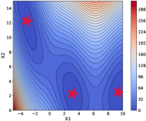
Figure 4: Branin function.

To assess the capability of DiffOPT  in optimizing functions under unknown constraints, we generate a dataset of 6,000 points, uniformly distributed within the feasible domain shaped like an oval. An effective optimizer is expected to infer the feasible space from the dataset and yield solutions strictly within the permissible region, i.e., $(-\pi,12.275)$ and $(\pi,2.275)$. We train a diffusion model with Variance Preserving (VP) SDE (Song et al., 2020) on this dataset. More details of the experimental setup are provided in Appendix D. Figure 2 illustrates the sampling trajectory of DiffOPT, clearly demonstrating its capability in guiding the samples towards the optimal points confined to the feasible space.

Compatible with additional known constraints.

Our framework is also adaptable to scenarios with additional, known constraints $C^{\prime}$. In such instances, we introduce an extra objective function whose Boltzmann density is uniform within the constraint bounds and $0$ otherwise, i.e., $q^{\prime}(x)\propto\exp[\beta^{\prime}\cdot I(x\in C^{\prime})]$, with $I(\cdot)$ being the indicator function. To demonstrate this capability, we incorporate a closed-form linear constraint alongside the implicit constraint represented by the dataset. This new constraint narrows the feasible solutions to only $(\pi,2.275)$. As depicted in Figure 3, DiffOPT effectively navigates towards the sole viable minimizer within the constrained space delineated by the data-driven and explicitly stated constraints. This feature is particularly beneficial in practical applications, such as molecular optimization, where imposing additional spatial or structure constraints might be necessary during optimizing binding affinities with different protein targets (Du et al., 2022).

5.2 Offline Black-box Optimization

We further evaluate DiffOPT on the offline black-box optimization task, wherein a logged dataset is utilized to train a surrogate model that approximates the objective function. This task can be considered as optimization under unknown constraints because direct optimization of the surrogate model can potentially misguide the search towards regions where model predictions are less reliable. It is, therefore, crucial to take into account the feasible space as delineated by the training data to ensure that the optimization process remains anchored in regions where the surrogate model’s predictions are trustworthy. Following Krishnamoorthy et al. (2023), We conduct evaluation on DesignBench (Trabucco et al., 2022), including three continuous optimization tasks and three discrete optimization tasks. Superconductor is to optimize for finding a superconducting material with high critical temperature. Ant nad D’Kitty is to optimize the morphology of robots. TFBind8 and TFBind10 are to find a DNA sequence that maximizes binding affinity with specific transcription factors. ChEMBL is to optimize the drugs for a particular chemical property.

Baselines. We compare DiffOPT with multiple baselines, including gradient ascent, Bayesian optimization (GP-qEI) (Krishnamoorthy et al., 2023), REINFORCE (Sutton et al., 1999), evolutionary algorithm (CAM-ES) (Hansen, ), and recent methods like MINS (Kumar & Levine, 2020), COMs (Trabucco et al., 2021a), CbAS (Brookes et al., 2019) and DDOM (Krishnamoorthy et al., 2023). We follow Krishnamoorthy et al. (2023) and set the sampling budget as $256$. More details of the experimental setups are provided in Appendix D.

Results. Table 1 shows the performance on the six datasets for all the methods. As we can see, DiffOPT achieves an average rank of $2.0$, the best among all the methods. We achieve the best result on 4 tasks. Particularly, in the Superconductor task, DiffOPT surpasses all baseline methods by a significant margin, improving upon the closest competitor by 9.6%. The exceptional performance of DiffOPT is primarily due to its application of a diffusion model to learn the valid data manifold directly from the data set, thus rendering the optimization process significantly more reliable. In contrast, the gradient ascent method, which relies solely on optimizing the trained surrogate model, is prone to settle on suboptimal solutions. Moreover, while DDOM (Krishnamoorthy et al., 2023) employs a conditional diffusion model to learn an inverse mapping from objective values to the input space, its ability to generate samples is confined to the maximum values present in the offline dataset. This limitation restricts its ability to identify global maximizers within the feasible space. The experimental results also demonstrate that DiffOPT can consistently outperform DDOM except for the Ant Dataset. On Ant, we find that the suboptimal performance of DiffOPT is because the surrogate model is extremely difficult to train. We provide more analyses in Appendix E.

5.3 Multi-objective Molecule Optimization

To showcase the performance of DiffOPT in multi-objective optimization, we test it on a molecule optimization task. In this task, we have three objectives: the maximization of the quantitative estimate of drug-likeness (QED), and the activity against glycogen synthase kinase three beta enzyme (GSK3B), and the minimization of the synthetic accessibility score (SA). Following Jin et al. (2020); Eckmann et al. (2022), we utilize a pre-trained autoencoder from Jin et al. (2020) to map discrete molecular structures into a continuous low-dimensional latent space and train neural networks as proxy functions for predicting molecular properties to guide the optimization. The detailed experimental setups are provided in Appendix D.

Results. For each method, we generate 1,000 candidate solutions, evaluating the three objective metrics solely on those that are valid. As we can see from Table 2, DiffOPT can achieve the best validity performance among all the methods. In terms of optimization performance, DiffOPT can achieve the best overall objective value. We further report the average of the top 10 solutions found by each model and find that DiffOPT is also reliable in this scenario. This multi-objective optimization setting is particularly challenging, as different objectives can conflict with each other. The superior performance of DiffOPT is because we formulate the optimization problem as a sample problem from the product of experts, which is easy for compositions of various objectives.

5.4 Ablation Study

In this section, we conduct ablation studies to explore the impact of annealing strategies and two-stage sampling. We also study the effect of training data size in Appendix F.

Impact of annealing strategies. We first study the influence of different annealing strategies for $\beta$ during the guided diffusion stage, focusing on the superconductor and TFBind8 datasets. We explore three strategies: constant, linear annealing, and exponential annealing. Figure 5(a) presents the performance across various diffusion steps. We find that our method is not particularly sensitive to the annealing strategies. However, it is worth noting that exponential annealing exhibits a marginal performance advantage over the others.

We also investigate how the value of $\beta$ at the end of annealing, denoted as $\beta_{\rm max}$, affects model performance in Figure 5(b). We find that increasing $\beta_{\rm max}$ initially leads to better performance. However, beyond a certain threshold, performance begins to decrease. It is noteworthy that the optimal value varies across different annealing strategies. Particularly, at $\beta_{\rm max}=0$, the model reverts to a pure diffusion process, exhibiting the lowest performance due to the lack of guidance from the objective function.

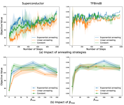
Figure 5: Impact of annealing strategies and $\beta_{\rm max}$ in the guided diffusion stage. $\beta_{\rm max}$ is the value of $\beta$ at the end of annealing.

Impact of two-stage sampling. Table 3 shows the impact of two-stage sampling on performance. Our findings reveal that even after the initial stage, DiffOPT outperforms the top-performing baseline on both datasets. Relying solely on Langevin dynamics, without the warm-up phase of guided diffusion, results in significantly poorer results. This aligns with our discussion in Section 3.2, where we attributed this failure to factors such as the starting distribution, the schedule for step size adjustments, and the challenges posed by undefined gradients outside the feasible set. Integrating both stages yields a performance improvement as the initial stage can provide a better initialization within the data manifold for the later stage (Theorem 1). Adding the Metropolis-Hastings (MH) correction step further enhances results, leading to the best performance observed.

	Superconductor	TFBind8
Best Baseline	$103.600\pm 8.139$	$0.981\pm 0.010$
Only Stage I	$112.038\pm 6.783$	$0.984\pm 0.012$
Only Stage II	$92.432\pm 8.635$	$0.951\pm 0.028$
Stage I + Stage II	$113.545\pm 5.322$	$0.987\pm 0.014$
Stage I + Stage II + MH	$\textbf{114.945}\pm 3.615$	$\textbf{0.989}\pm 0.021$

Table 3: Ablation study on the two-stage sampling.

6 Conclusion, Limitation, and Future Work

In this paper, we propose DiffOPT to solve the optimization problems where analytic constraints are unavailable. We propose to learn the unknown feasible space from data using a diffusion model and then reformulate the original problem as a sampling problem from the product of (i) the density of the data distribution learned by the diffusion model, and (ii) the Boltzmann density defined by the objective function. For effective sampling, we propose a two-stage framework which consists of a guided diffusion stage for warm-up and a Langevin dynamics stage for further correction. Theoretical analysis demonstrates that the guided diffusion provides better initialization for the later Langevin dynamics sampling. Our experiments have validated the effectiveness of DiffOPT.

We discuss limitations and possible extensions of DiffOPT. (i) Manifold preserving. The guided diffusion may deviate from the manifold that the score network is trained, leading to error accumulations. One approach to mitigate this is to incorporate manifold constraints during the guided diffusion phase (Chung et al., 2022b; He et al., 2023). (ii) Ensuring hard constraints. We can only satisfy soft constraints for the additional known constraints. However, one could directly constrain the diffusion space (Lou & Ermon, 2023; Fishman et al., 2023; Liu et al., 2023). (iii) Extension to derivative-free optimization. Diffusion can also be utilized to tackle derivative-free optimization which does not require a surrogate model (Engquist et al., 2024).

7 Impact Statement

Optimization techniques can be used to solve a wide range of real-world problems, from decision making (planning, reasoning, and scheduling), to solving PDEs, and to designing new drugs and materials. The method we present in this paper extends the scope of the previous study to a more realistic setting where (partial) constraints for optimization problems are unknown, but we have access to samples from the feasible space. We expect that by learning the feasible set from data, our work can bring a positive impact to the community in accelerating solving real-world optimization problems and finding more realistic solutions. However, care should be taken to prevent the method from being used in harmful settings, such as optimizing drugs to enhance detrimental side effects.

8 Acknowledgement

Y.D. would like to thank Yunan Yang, Guan-horng Liu, Ricky T.Q. Chen, Ge Liu and Yimeng Zeng for their helpful discussions.

Appendix for DiffOPT

[sections] [sections]l1

Appendix A (Metropolis-adjusted) Langevin Dynamics.

Langevin dynamics is a class of Markov Chain Monte Carlo (MCMC) algorithms that aims to generate samples from an unnormalized density $\pi(x)$ by simulating the differential equation

$$\textnormal{d}\mathbf{x}_{t}=\nabla_{\mathbf{x}}\log\pi(\mathbf{x}_{t})\textnormal{d}t+\sqrt{2}\textnormal{d}\mathbf{w}_{t}.$$ (14)

Theoretically, the continuous SDE of Equation 14 is able to draw exact samples from $\pi(x)$. However, in practice, one needs to discretize the SDE using numerical methods such as the Euler-Maruyama method (Kloeden et al., 1992) for simulation. The Euler-Maruyama approximation of Equation 14 is given by

$$x_{t+\Delta t}=x_{t}+\nabla\log\pi(x)+\sqrt{2\Delta t}z,\qquad z\sim\mathcal{N}(0,1),$$ (15)

where $\Delta t$ is the step size. By drawing $x_{0}$ from an initial distribution and then simulating the dynamics in Equation 14, we can generate samples from $\pi(x)$ after a ’burn-in’ period. This algorithm is known as the Unadjusted Langevin Algorithm (ULA) (Roberts & Tweedie, 1996), which requires $\nabla\log\pi(x)$ to be $L$-Lipschitz for stability.

The ULA always accepts the new sample proposed by Equation 15. In contrast, to mitigate the discretization error when using a large step size, the Metropolis-adjusted Langevin Algorithm (MALA) (Grenander & Miller, 1994) uses the Metropolis-Hastings algorithm to accept or reject the proposed sample. Specifically, we first generate a proposed update $\hat{x}$ with Equation 14, then with probability $\text{min}(1,\frac{\pi(\hat{x})\mathcal{N}(x|\hat{x}+\Delta t\cdot\nabla_{\hat{x}}\log\pi(\hat{x}),2\Delta t)}{\pi(x)\mathcal{N}(\hat{x}|x+\Delta t\cdot\nabla_{x}\log\pi(x),2\Delta t)}$), we set $x_{t+\Delta t}=\hat{x}$, otherwise $x_{t+\Delta}=x_{t}$. We provide the pseudocode of both algorithms in Algorithm 2.

Algorithm 2 Sampling via the (Metropolis-Adjusted) Langevin dynamics

0:  unnormalized density $\pi(x)$, step size $\Delta t$

1:  $x\sim\text{initial distribution}$

2:  $\mathcal{X}=\varnothing$

3:  for number of iterations do

4:     $\hat{x}=x+\nabla_{x}\log\pi(x)\Delta t+\sqrt{2\Delta t}\cdot z,\;\;z\sim\mathcal{N}(0,1)$

5:     if applying Metropolis-Hastings test then

6:        $u\sim\text{Uniform}[0,1]$

7:        $\log P_{\text{accept}}=\log\frac{\pi(\hat{x})\mathcal{N}(x|\hat{x}+\Delta t\cdot\nabla_{\hat{x}}\log\pi(\hat{x}),2\Delta t)}{\pi(x)\mathcal{N}(\hat{x}|x+\Delta t\cdot\nabla_{x}\log\pi(x),2\Delta t)}$

8:        $\text{if }\;\;\log P_{\text{accept}}>\log u,\;\;\text{ then }\;\;x\leftarrow\hat{x}$

9:     else

10:        $x\leftarrow\hat{x}$

11:     end if

12:     $\mathcal{X}\leftarrow\mathcal{X}\cup x$

13:  end for

13:  $\mathcal{X}$

Appendix B Energy-based Parameterization

In a standard diffusion model, we learn the score of the data distribution directly as $s_{\theta}(x,t)=\nabla\log p_{t}(x)$. This parameterization can be used for ULA, which only requires gradients of log-likelihood. However, to incorporate the Metropolis-Hastings (MH) correction step, access to the unnormalized density of the data distribution is necessary to calculate the acceptance probability.

To enable the use of MH correction, we can instead learn the energy function of the data distribution, i.e., $p(x,t)\propto e^{E_{\theta}(x,t)}$. The simplest approach is to use a scalar-output neural network, denoted as $\text{NN}_{\theta}(x,t):\mathbb{R}^{d}\times\mathbb{R}\rightarrow\mathbb{R}$, to parameterize $E_{\theta}(x,t)$. By taking the gradient of this energy function with respect to the input $x$, we can derive the score of the data distribution. However, existing works have shown that this parameterization can cause difficulties during model training (Salimans & Ho, 2021). Following the approach by (Du et al., 2023b), we define the energy function as $E_{\theta}(x,t)=-\frac{1}{2}|\text{NN}_{\theta}(x,t)|^{2}_{2}$, where $\text{NN}_{\theta}(x,t)$ is a vector-output neural network mapping from $\mathbb{R}^{d}\times\mathbb{R}$ to $\mathbb{R}$. Consequently, the score of the data distribution is represented as $s_{\theta}(x,t)=-\text{NN}_{\theta}(x,t)\nabla_{x}\text{NN}_{\theta}(x,t)$.

Appendix C End Distribution of the Warm-up Stage

In this section, we study in further detail the warm-up stage of DiffOPT. We recall that we consider a process of the following form

$$\mathrm{d}\mathbf{y}_{t}^{\beta}=[-f(\mathbf{y}_{t}^{\beta},1-t)+g(1-t)^{2}\nabla\log p_{1-t}(\mathbf{y}_{t}^{\beta})-\beta(1-t)\nabla h(\mathbf{y}_{t}^{\beta})]\mathrm{d}t+g(1-t)\mathrm{d}\mathbf{w}_{t},\qquad\mathbf{y}_{0}^{\beta}\sim\mathbf{x}_{T}$$ (16)

where $T=1$ and $p_{t}$ is the density w.r.t. Lebesgue measure of the distribution of $\mathbf{x}_{t}$ where

$$\mathrm{d}\mathbf{x}_{t}=f(t,\mathbf{x}_{t})\mathrm{d}t+g(t)\mathrm{d}\mathbf{w}_{t},\qquad\mathbf{x}_{0}\sim p_{0}.$$ (17)

We recall that under mild assumption (Cattiaux et al., 2023), we have that $(\hat{\mathbf{y}}_{t})_{t\in[0,1]}=(\mathbf{x}_{1-t})_{t\in[0,1]}$ satisfies

$$\mathrm{d}\hat{\mathbf{y}}_{t}=[-f(\hat{\mathbf{y}}_{t},1-t)+g(1-t)^{2}\nabla\log p_{1-t}(\hat{\mathbf{y}}_{t})]\mathrm{d}t+g(1-t)\mathrm{d}\mathbf{w}_{t},\qquad\hat{\mathbf{y}}_{0}=\mathbf{x}_{T}.$$ (18)

Let us highlight some differences between (16) and the warm-up process described in Algorithm 1. First, we note that we do not consider an approximation of the score but the real score function $\nabla\log p_{t}$. In addition, we do not consider a discretization of (16). This difference is mainly technical. The discretization of diffusion processes is a well-studied topic, and we refer to (De Bortoli et al., 2021; Benton et al., 2023; Conforti et al., 2023; Chen et al., 2022) for a thorough investigation. Our contribution to this work is orthogonal as we are interested in the role of $h$ on the distribution. Our main result is Proposition 4 and details how the end distribution of the warm-up process concentrates on the minimizers of $h$, which also support the data distribution $p_{0}$.

We first show that under assumptions on $h$, $q_{T}^{\beta}$, the density w.r.t. the Lebesgue measure of $\mathbf{y}_{T}$ has the same support as $p_{0}$. We denote by $\mathrm{supp}(p_{0})$ the support of $p_{0}$. We consider the following assumption.

Assumption 1.

We have that for any $t\in[0,1]$, $g(t)=g(0)$ and $f(t,x)=-\gamma_{0}x$ with $\gamma_{0}>0$. Assume that $p_{0}$ has bounded support, i.e. there exists $R>0$ such that $\mathrm{supp}(p_{0})\subset\mathrm{B}(0,R)$ with $\mathrm{B}(0,R)$ the ball with center $0$. In addition, assume that $h$ is Lipschitz.

Then, we have the following proposition.

Proposition 2.

Assume A1. Then, we have that for any $\beta>0$, $\mathbf{y}_{T}^{\beta}\in\mathrm{supp}(p_{0})$.

Proof.

This directly applies to the results of (Pidstrigach, 2022). First, we have that Pidstrigach (2022, Assumption 1, Assumption 2) are satisfied using A1, Pidstrigach (2022, Lemma 1) and the second part of Pidstrigach (2022, Theorem 2). We conclude using the first part of Pidstrigach (2022, Theorem 2). ∎

In Proposition 2, we show that the guided reconstructed scheme used for warm-up (16) cannot discover minimizers outside the support of $p_{0}$. In Proposition 4, we will show that we concentrate on the minimizers inside the support of $p_{0}$ under additional assumptions.

Next, we make the following assumption, which is mostly technical. We denote $q_{t}^{\beta}$ the distribution of $\mathbf{y}_{t}^{\beta}$ for any $t\in[0,1]$. We also denote $(p_{1-t}^{\beta})_{t\in[0,1]}=(q_{t}^{\beta})_{t\in[0,1]}$.

Assumption 2.

We have that $h\in\mathrm{C}^{\infty}(\mathbb{R}^{d},\mathbb{R})$. In addition, $C>0$ exists such that for any $x\in\mathbb{R}^{d}$ and $\beta_{0}>0$, we have a.s.

$$\textstyle|\int_{\beta}^{1}(1/t)(W_{t}^{\beta}(\mathbf{z}_{t})-W_{0}^{\beta}(\mathbf{z}_{0}))\mathrm{d}t|\leq C,$$ (19)

with $\mathrm{d}\mathbf{z}_{t}=\{f_{t}-g_{t}^{2}\nabla\log p_{t}\rangle\mathrm{d}t+\mathrm{d}\mathbf{w}_{t}$, $\mathbf{z}_{0}=x$ and $W_{t}=\langle\nabla\log p_{t}^{\beta},\nabla h\rangle+\Delta h$. For any $\beta_{0}>0$, $t\in[0,1]$ and $x\in\mathbb{R}^{d}$

$$V_{t}=\mathrm{div}(f_{t}-g_{t}^{2}\nabla\log p_{t}),\qquad W_{t}^{\beta}=\langle\nabla h,\nabla\log p_{t}^{\beta}\rangle+\Delta h.$$ (20)

Assume that $V$ and $W^{\beta}$ are continuous and bounded on $[0,1]\times\mathbb{R}^{d}$. Assume that $(p_{t})_{t\in[0,1]}$ and $(p_{t}^{\beta})_{t\in[0,1]}$ are strong solutions to their associated Fokker-Planck equations.

We do not claim that we verify this hypothesis in this paper. Proving A2 is out of the scope of this work, and we mainly use it to 1) control high-order terms and 2) provide sufficient conditions to apply the Feynman-Kac theorem Oksendal (2013, Theorem 7.13) and the Fokker-Planck equation. The bound in (19) controls the regularity of the $W_{t}^{\beta}(\mathbf{z}_{t})$. Given that (under some mild regularity assumption), $(W_{t}^{\beta}(\mathbf{z}_{t}))_{t\in[0,1]}$ satisfies a Stochastic Differential Equation we expect that $\mathbb{E}[\|(W_{t}^{\beta}(\mathbf{z}_{t})-W_{0}^{\beta}(\mathbf{z}_{0}))\|]\leq C\sqrt{t}$ for any $t\in[0,1]$ and some constant $C>0$ (independent of $t$). Therefore, we get that (19) is true in expectation under some regularity assumption. We conjecture that the almost sure bound we require is unnecessary and that moment bounds should be enough. We leave this study for future work.

Proposition 3.

Assume A2 and that $\beta(t)=1/t$ if $t>1/\beta_{0}$ and $0$ otherwise. For any $x\in\mathbb{R}^{d}$, let $\tilde{p}_{0}^{\beta}(x)$ be given by

$$\tilde{p}_{0}^{\beta}(x)=p_{0}(x)\exp[\log(\beta_{0})\{\Delta h(x)+\langle\nabla\log p_{0}^{\beta}(x),\nabla h(x)\rangle\}],$$ (21)

where $p_{0}^{\beta}$ is the distribution of $\mathbf{y}_{T}^{\beta}$. Then there exists $C_{0}>0$ such that for any $x\in\mathbb{R}^{d}$

$$(1/C_{0})\tilde{p}_{0}^{\beta}(x)\leq p_{0}^{\beta}(x)\leq C_{0}\tilde{p}_{0}^{\beta}(x).$$ (22)

Before diving into the proof, let us provide some insight on Proposition 3. The distribution of $p_{0}^{\beta}$ is the distribution of interest as it is the output distribution of the guided warm-up process. We consider a specific schedule $\beta(t)=1/t$ with $t>t_{0}$ and $0$ otherwise to obtain meaningful bounds. This means that as $\beta_{0}\to\infty$, we are increasingly emphasizing $t\approx 0$.

Proof.

First, for any $t\in[0,1]$ we denote $p_{t}$ the density of $\mathbf{x}_{t}$ where $(\mathbf{x}_{t})_{t\in[0,1]}$ is given by (17). Similarly, we denote $q_{t}^{\beta}$ the distribution of $\mathbf{y}_{t}^{\beta}$ for any $\tau_{0}>0$ and $t\in[0,1]$. Finally, we denote $(p_{1-t}^{\beta})_{t\in[0,1]}=(q_{t}^{\beta})_{t\in[0,1]}$ for any $\tau_{0}>0$. In what follows, we fix $t_{0}>0$. Using A2 we have that for any $t\in[0,1]$

$$\partial_{t}p_{t}=-\mathrm{div}(f_{t}p_{t})+(g_{t}^{2}/2)\Delta p_{t}.$$ (23)

Therefore, we have that for any $t\in[0,1]$

$$\partial_{t}p_{t}+\mathrm{div}(f_{t}p_{t})-(g_{t}^{2}/2)\Delta p_{t}=0.$$ (24)

This can also be rewritten as

$$\partial_{t}p_{t}+\langle f_{t}-g_{t}^{2}\nabla\log p_{t},\nabla p_{t}\rangle+(g_{t}^{2}/2)\Delta p_{t}+\mathrm{div}(f_{t}-g_{t}^{2}\nabla\log p_{t})p_{t}=0,$$ (25)

where we have used that $\mathrm{div}(\nabla\log p_{t}p_{t})=\Delta p_{t}$. Similarly, we have that

$$\partial_{t}q_{t}^{\beta}=-\mathrm{div}(\{-f_{1-t}+g_{1-t}^{2}\nabla\log p_{1-t}-\beta_{1-t}\nabla h\}q_{t}^{\beta})+(g_{1-t}^{2}/2)\Delta q_{t}^{\beta}.$$ (26)

We have that

$$\partial_{t}p_{t}^{\beta}=\mathrm{div}(\{-f_{t}+g_{t}^{2}\nabla\log p_{t}-\beta_{t}\nabla h\}p_{t}^{\beta})-(g_{t}^{2}/2)\Delta p_{t}^{\beta}.$$ (27)

This can also be rewritten as

$$\partial_{t}p_{t}^{\beta}+\langle f_{t}-g_{t}^{2}\nabla\log p_{t}^{\beta},\nabla p_{t}^{\beta}\rangle+\mathrm{div}(f_{t}-g_{t}^{2}\nabla\log p_{t})p_{t}^{\beta}+(g_{t}^{2}/2)\Delta p_{t}^{\beta}+\mathrm{div}(\beta_{t}\nabla hp_{t}^{\beta})=0.$$ (28)

Finally, this can be rewritten as

$$\partial_{t}p_{t}^{\beta}+\langle f_{t}-g_{t}^{2}\nabla\log p_{t},\nabla p_{t}^{\beta}\rangle+(g_{t}^{2}/2)\Delta p_{t}^{\beta}+\mathrm{div}(f_{t}-g_{t}^{2}\nabla\log p_{t})p_{t}^{\beta}+\beta_{t}\{\langle\nabla h,\nabla\log p_{t}^{\beta}\rangle+\Delta h\}p_{t}^{\beta}=0.$$ (29)

In what follows, we denote

$$\mu_{t}=f_{t}-g_{t}^{2}\nabla\log p_{t},\qquad V_{t}=\mathrm{div}(f_{t}-g_{t}^{2}\nabla\log p_{t}),\qquad W_{t}^{\beta}=\langle\nabla h,\nabla\log p_{t}^{\beta}\rangle+\Delta h.$$ (30)

Hence, using (28) we have

$$\partial p_{t}^{\beta}+\langle\mu_{t},\nabla\log p_{t}^{\beta}\rangle+(g_{t}^{2}/2)\Delta p_{t}^{\beta}+V_{t}p_{t}^{\beta}+\beta_{t}W_{t}^{\beta}p_{t}^{\beta}=0.$$ (31)

Similarly, using (25) we have

$$\partial p_{t}+\langle\mu_{t},\nabla\log p_{t}\rangle+(g_{t}^{2}/2)\Delta p_{t}+V_{t}p_{t}=0.$$ (32)

Therefore, combining (32), A2 and Oksendal (2013, Theorem 7.13) we get that for any $x\in\mathbb{R}^{d}$

$$\textstyle p_{0}(x)=\mathbb{E}[\exp[\int_{0}^{1}V_{t}(\mathbf{z}_{t})\mathrm{d}t]p_{T}(\mathbf{z}_{T})\ |\ \mathbf{z}_{0}=x],$$ (33)

with $\mathrm{d}\mathbf{z}_{t}=\mu_{t}\mathrm{d}t+g_{t}\mathrm{d}\mathbf{w}_{t}$ and $\mathbf{z}_{0}=x$. Similarly, combining (31), A2 and Oksendal (2013, Theorem 7.13) we get that for any $x\in\mathbb{R}^{d}$

$$\textstyle p_{0}^{\beta}(x)=\mathbb{E}[\exp[\int_{0}^{1}V_{t}(\mathbf{z}_{t})\mathrm{d}t]\exp[\int_{0}^{1}\beta_{t}W_{t}^{\beta}(\mathbf{z}_{t})\mathrm{d}t]p_{T}(\mathbf{z}_{T})\ |\ \mathbf{z}_{0}=x].$$ (34)

Using (30), we have that

$$\textstyle\int_{0}^{1}\beta_{t}W_{t}^{\beta}(\mathbf{z}_{t})\mathrm{d}t=\int_{1/\beta_{0}}^{1}(1/t)\{\langle\nabla h,\nabla\log p_{t}^{\beta}\rangle+\Delta h\}(\mathbf{z}_{t})\mathrm{d}t.$$ (35)

Hence, we have

$$\textstyle\int_{0}^{1}\beta_{t}W_{t}^{\beta}(\mathbf{z}_{t})\mathrm{d}t=\log(\beta_{0})\{\langle\nabla h,\nabla\log p_{0}^{\beta}\rangle+\Delta h\}(\mathbf{z}_{0})+\int_{1/\beta_{0}}^{1}(1/t)(W_{t}^{\beta}(\mathbf{z}_{t})-W_{0}^{\beta}(\mathbf{z}_{0}))\mathrm{d}t.$$ (36)

Using A2 we have that

$$-C\leq\textstyle\int_{0}^{1}\beta_{t}W_{t}^{\beta}(\mathbf{z}_{t})\mathrm{d}t-\log(\beta_{0})\{\langle\nabla h,\nabla\log p_{0}^{\beta}\rangle+\Delta h\}(\mathbf{z}_{0})\leq C\,.$$ (37)

Hence,

$$-C+\log(\beta_{0})\{\langle\nabla h,\nabla\log p_{0}^{\beta}\rangle+\Delta h\}(\mathbf{z}_{0})\leq\textstyle\int_{0}^{1}\beta_{t}W_{t}^{\beta}(\mathbf{z}_{t})\mathrm{d}t\leq C+\log(\beta_{0})\{\langle\nabla h,\nabla\log p_{0}^{\beta}\rangle+\Delta h\}(\mathbf{z}_{0})\,.$$ (38)

Combining this result with (34) we get that for any $x\in\mathbb{R}^{d}$

$$\textstyle p_{0}^{\beta}(x) \leq\textstyle\mathbb{E}[\exp[\int_{0}^{1}V_{t}(\mathbf{z}_{t})\mathrm{d}t]p_{T}(\mathbf{z}_{T})\ |\ \mathbf{z}_{0}=x]\exp[\log(\beta_{0})\{\langle\nabla h,\nabla\log p_{0}^{\beta}+\Delta h\rangle\}(x)]\exp[C]$$ (39)

$$=p_{0}(x)\exp[\log(\beta_{0})\{\langle\nabla h,\nabla\log p_{0}^{\beta}+\Delta h\rangle\}(x)]\exp[C].$$ (40)

Similarly, we have for any $x\in\mathbb{R}^{d}$

$$\textstyle p_{0}^{\beta}(x)\geq p_{0}(x)\exp[\log(\beta_{0})\{\langle\nabla h,\nabla\log p_{0}^{\beta}\rangle+\Delta h\}(x)]\exp[-C],$$ (41)

which concludes the proof. ∎

While Proposition 3 gives an explicit form for $p_{0}^{\beta}$, it does not provide insights on the properties of this distribution. However, we can still infer some limiting properties.

Proposition 4.

If $x^{\star}$ is a local strict minimizer of $h$ in the support of $p_{0}$ then $\lim_{\beta_{0}\to\infty}p_{0}^{\beta}(x^{\star})=+\infty$. If $x^{\star}$ is a local strict minimizer of $h$ not in the support of $p_{0}$ then $\lim_{\beta_{0}\to\infty}p_{0}^{\beta}(x^{\star})=0$.

Proof.

The case where $x^{\star}$ is not in support of $p_{0}$ is trivial using Proposition 3. We now assume that $x^{\star}$ is in the support of $p_{0}$. Using Proposition 3 and that $\nabla h(x^{\star})=0$ and $\Delta h(x^{\star})>0$ since the local minimizer $x^{\star}$ is strict, we get that $\lim_{\beta_{0}\to\infty}p_{0}^{\beta}(x^{\star})=+\infty$, which concludes the proof. ∎

In particular, Proposition 4 shows that the limit distribution of $\mathbf{y}_{T}^{\beta}$ concentrates around the minimizers of $h$, which is the expected behavior of increasing the inverse temperature. What is also interesting is that we only target the minimizers of $h$, which are inside the support of $p_{0}$. This is our primary goal, which is constrained optimization of $h$.

Appendix D Experiment Details

D.1 Synthetic Branin Experiment

We consider the commonly used Branin function as a synthetic toy example that takes the following form (illustrated in Figure 4):

$$f(x_{1},x_{2})=a(x_{2}-bx_{1}^{2}+cx_{1}-r)^{2}+s(1-t)\text{cos}(x_{1})+s,$$ (42)

where $a=1$, $b=\frac{5.1}{4\pi^{2}}$, $c=\frac{5}{\pi}$, $r=6$, $s=10$, $t=\frac{1}{8\pi}$.

The Branin function $f(x_{1},x_{2})$ has three global minimas located at points $(-\pi,12.275)$, $(\pi,2.275)$, and $(9.42478,2.475)$ with a value of $0.397887$.

Dataset details. We curate $6,000$ data points by sampling uniformly in an ellipse region with center $(-0.2,7.5)$ and semi-axis lengths $(3.6,8.0)$ as training data (the blue region in Figure 2). It is tilted counterclockwise by 25 degrees, ensuring that it covers two minimizers of the function: $(-\pi,12.275)$ and $(\pi,2.275)$. It is worth noting that sampling points $(x_{1},x_{2})$ to construct the training dataset are irrelevant to the objective value $f(x_{1},x_{2})$. For the experiment with additional known constraints, we introduce two constraints $x_{2}\leq\frac{3}{2}x_{1}+\frac{15}{2}$ and $x_{2}\leq-\frac{3}{2}x_{1}+15$ (the pink region in Figure 2) to further narrow down the feasible solution to $(\pi,2.275)$. We split the dataset into training and validation sets by 9:1.

Implementation details. We build the score network $s_{\theta}$ of the diffusion model with a 2-layer MLP architecture with 1024 hidden dimensions and ReLU activation function. The forward process is a Variance Preserving (VP) SDE (Song et al., 2020). We set the minimum and maximum values of noise variance to be $0.01$ and $2.0$, respectively. We employ a fixed learning rate of $0.001$, a batch size of $128$, and $1000$ epochs for model training. At test time, we sample $500$ candidate solutions. We use a constant inverse temperature $\beta=5$ for the Boltzmann distribution induced by the objective function. For the distribution induced by the additional known constraints, we set $\beta^{\prime}=10.$

D.2 Offline Black-box Optimization

Dataset details. DesignBench (Trabucco et al., 2022) is an offline black-box optimization benchmark for real-world optimization tasks. Following Krishnamoorthy et al. (2023), we use three continuous tasks: Superconductor, D’Kitty Morphology and Ant Morphology, and three discrete tasks: TFBind8, TFBind10, and ChEMBL. Consistent with Krishnamoorthy et al. (2023), we exclude NAS due to its significant computational resource demands. We also exclude Hopper as it is known to be buggy (see Appendix C in Krishnamoorthy et al. (2023)). We split the dataset into training and validation sets by 9:1.

• Superconductor: materials optimization. This task aims to search for materials with high critical temperatures. The dataset contains 17,014 vectors with 86 components representing the number of atoms of each chemical element in the formula. The provided oracle function is a pre-trained random forest regression model.

• D’Kitty Morphology: robot morphology optimization. This task aims to optimize the parameters of a D’Kitty robot, such as size, orientation, and location of the limbs, to make it suitable for a specific navigation task. The dataset size is 10,004, and the parameter dimension is 56. It uses MuJoCO (Todorov et al., 2012), a robot simulator, as the oracle function.

• Ant Morphology: robot morphology optimization. Similar to D’Kitty, this task aims to optimize the parameters of a quadruped robot to move as fast as possible. It consists of 10,004 data, and the parameter dimension is 60. It also uses MuJoCo as the oracle function.

• TFBind8: DNA sequence optimization. This task aims to find the DNA sequence of length eight with the maximum binding affinity with transcription factor SIX6_REF_R1. The design space is the space of sequences of nucleotides represented as categorical variables. The size of the dataset is 32,898, with a dimension of 8. The ground truth serves as a direct oracle since the affinity for the entire design space is available.

• TFBind10: DNA sequence optimization. Similar to TFBind8, this task aims to find the DNA sequence of length ten that has the maximum binding affinity with transcription factor SIX6_REF_R1. The design space consists of all possible designs of nucleotides. The size of the dataset is 10,000, with a dimension of 10. Since the affinity for the entire design space is available, it uses the ground truth as a direct oracle.

• ChEMBL: molecule activity optimization. This task aims to find molecules with a high MCHC value when paired with assay CHEMBL3885882. The dataset consists of 441 samples of dimension 31.

Baselines. We compare with eight baselines on DesignBench tasks. The results of all the baselines are from Krishnamoorthy et al. (2023). Gradient ascent learns a surrogate model of the objective function and generates the optimal solution by iteratively performing gradient ascent on the surrogate model. CbAS learns a density model in the design space coupled with a surrogate model of the objective function. It iteratively generates samples and refines the density model on the new samples during training. GP-qEI fits a Gaussian Process on the offline dataset. It employs the quasi-Expected-Inprovement (qEI) acquisition function from Botorch  (Baladat et al., 2020) for Bayesian optimization. MINS learns an inverse map from objective value back to design space using a Generative Adversarial Network (GAN). It then obtains optimal solutions through conditional generation. REINFORCE parameterizes a distribution over the design space and adjusts this distribution in a direction that maximizes the efficacy of the surrogate model. COMS learns a conservative surrogate model by regularizing the adversarial samples. It then utilizes gradient ascent to discover the optimal solution. CMAES enhances a distribution over the optimal design by adapting the covariance matrix according to the highest-scoring samples selected by the surrogate model. DDOM learns a conditional diffusion model to learn an inverse mapping from the objective value to the input space.

Implementation details. We build the score network $s_{\theta}$ using a simple feed-forward network. This network consists of two hidden layers, each with a width of 1024 units, and employs ReLU as the activation function. The forward process is a Variance Preserving (VP) SDE (Song et al., 2020). We set the noise variance limits to a minimum of 0.01 and a maximum of 2.0.

For the surrogate models, we explore various network architectures tailored to different datasets, including Long short-term memory (LSTM) (Hochreiter & Schmidhuber, 1997), Gaussian Fourier Network, and Deep Kernel Learning (DKL) (Wilson et al., 2016a, b). LSTM network uses a single-layer LSTM unit with a hidden dimension of 1024, followed by 1 hidden layer with a dimension of 1024, utilizing ReLU as the activation function. In the Gaussian Fourier regressor, Gaussian Fourier embeddings (Tancik et al., 2020) are applied to the inputs $x$ and $t$. These embeddings are then processed through a feed-forward network with 3 hidden layers, each of 1024 width, utilizing Tanh as the activation function. This regressor is time-dependent, and its training objective follows the method used by Song et al. (2020) for training time-dependent classifiers in conditional generation. For DKL, we use the ApproximateGP class in Gpytorch, which consists of a deep feature extractor and a Gaussian process (GP). The feature extractor is a simple feed-forward network consisting of $2$ hidden layers with a width of $500$ and $50$, respectively, and ReLU activations. The GP uses radial basis function (RBF) kernel.

We use a fixed learning rate of 0.001 and a batch size of 128 for both the diffusion and surrogate models. During testing, we follow the evaluation protocol from the (Krishnamoorthy et al., 2023), sampling 256 candidate solutions. We apply different annealing strategies for different datasets. Specifically, we apply exponential annealing for TFBind8, superconductor, D’Kitty, and ChEMBL. The exponential annealing strategy is defined as $\beta(\tau)=\beta_{\rm max}[1-\exp(-100(T-\tau))]$, where $\tau=T-t$, and a constant $\beta$ for Ant and TFBind10. Though exponential annealing usually exhibits better performance, we leave the exploration of exponential annealing on TFBind10 and D’Kitty for future work due to time limit. The step size $\Delta t$ is $0.001$ for the first stage, and $0.0001$ for the second stage.

Detailed hyperparameters and network architectures for each dataset are provided in Table 4.

	Annealing strategy	$\beta_{\rm max}$	Surrogate model
TFBind8	Exponential	$200$	Gaussian Fourier
TFBind10	Constant	$20$	Gaussian Fourier
Superconductor	Exponential	$100$	Gaussian Fourier
Ant	Exponential	30	Gaussian Fourier
D’Kitty	Constant	$3e4$	DKL
ChEMBL	Exponential	$100$	LSTM

Table 4: Implementation details on design-bench. $\beta_{\rm max}$ is the value of $\beta$ at the end of the annealing process.

D.3 Multi-objective Molecule Optimization

Dataset details. We curate the dataset by encoding 10000 molecules (randomly selected) from the ChEMBL dataset (Gaulton et al., 2012) with HierVAE (Jin et al., 2020), a commonly used molecule generative model based on VAE, which takes a hierarchical procedure in generating molecules by building blocks. Since validity is important for molecules, we ensure HierVAE can decode all the randomly selected encoded molecules. We split all the datasets into training and validation sets by 9:1.

Oracle details. We evaluate three commonly used molecule optimization oracles including synthesis accessibility (SA), quantitative evaluation of drug-likeness (QED) and activity again target GSK3B from RDKit (Landrum et al., 2020) and TDC (Huang et al., 2021). All three oracles take as input a SMILES string representation of a molecule and return a scalar value of the property. The oracles are non-differentiable.

Implementation details. We build the score network $s_{\theta}$ of the diffusion model using a 2-layer MLP architecture. This network features 1024 hidden dimensions and utilizes the ReLU activation function. The forward process adheres to a Variance Preserving (VP) SDE proposed by  (Song et al., 2020). We calibrate the noise variance within this model, setting its minimum at $0.01$ and maximum at $2.0$.

For the surrogate model of the objective function, we use the ApproximateGP class in Gpytorch, which consists of a deep feature extractor and a Gaussian process. The feature extractor is a simple feed-forward network with two hidden layers, having widths of 500 and 50, respectively, and both employ ReLU activation functions. Regarding model optimization, we apply a fixed learning rate of $0.001$ for the diffusion model and $0.01$ for the surrogate model. Additionally, we set a batch size of 128 and conduct training over 1000 epochs for both models. For the sampling process, we use a consistent inverse temperature $\beta=10^{4}$ for all the three objectives. The step size $\Delta t$ is $0.001$ for the first stage, and $0.0001$ for the second stage.

We sample $1000$ candidate solutions at test time for all the methods. For DDOM (Krishnamoorthy et al., 2023), we use their implementation . For other baselines, we use the implementations provided by DesignBench. We tune the hyper-parameters of all the baselines as suggested in their papers.

Appendix E Analysis on Ant Dataset

As shown in Table 1, DiffOPT can only achieve subpar performance on the Ant dataset. This underperformance is primarily due to the difficulty in training the surrogate objective function. An illustration of this challenge is provided in Figure 6, where the training loss of the surrogate objective is displayed. The training loss fluctuates throughout the training process. Although we investigated different network architectures, the issue still remains. Building an effective surrogate model for this dataset may require a more sophisticated architecture design. We leave this for future work.

Appendix F Impact of Training Data Size

Impact of training data size.

We finally investigate the impact of training data size on the superconductor dataset. We compare DiffOPT with the best baseline on this dataset—DDOM. As we can see from Figure 7, DiffOPT outperforms DDOM constantly across all the ratios of training data.

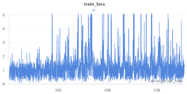
Figure 6: Training loss of the surrogate objective on Ant dataset

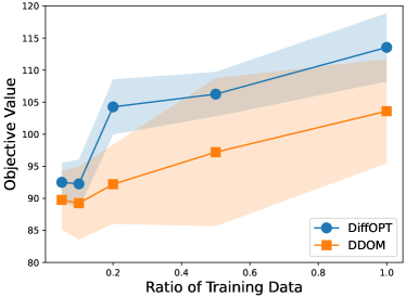
Figure 7: Impact of the number of training data.

References

- Alarie et al. (2021) Alarie, S., Audet, C., Gheribi, A. E., Kokkolaras, M., and Le Digabel, S. Two decades of blackbox optimization applications. EURO Journal on Computational Optimization, 9:100011, 2021.
- Anderson (1982) Anderson, B. D. Reverse-time diffusion equation models. Stochastic Processes and their Applications, 12(3):313–326, 1982.
- Baladat et al. (2020) Baladat, M., Karrer, B., Jiang, D. R., Daulton, S., Letham, B., Wilson, A. G., and Bakshy, E. Botorch: Programmable bayesian optimization in pytorch. Advances in Neural Information Processing Systems, 2020.
- Baran (2018) Baran, P. S. Natural product total synthesis: as exciting as ever and here to stay, 2018.
- Bazaraa et al. (2011) Bazaraa, M. S., Jarvis, J. J., and Sherali, H. D. Linear programming and network flows. John Wiley & Sons, 2011.
- Benton et al. (2023) Benton, J., De Bortoli, V., Doucet, A., and Deligiannidis, G. Linear convergence bounds for diffusion models via stochastic localization. arXiv preprint arXiv:2308.03686, 2023.
- Boyd & Vandenberghe (2004) Boyd, S. P. and Vandenberghe, L. Convex optimization. Cambridge university press, 2004.
- Branke & Schmidt (2004) Branke, J. and Schmidt, C. Sequential sampling in noisy environments. In International Conference on Parallel Problem Solving from Nature, pp. 202–211. Springer, 2004.
- Brookes et al. (2019) Brookes, D. H., Park, H., and Listgarten, J. Conditioning by adaptive sampling for robust design. International Conference on Machine Learning, 2019.
- Burke et al. (2005) Burke, J. V., Lewis, A. S., and Overton, M. L. A robust gradient sampling algorithm for nonsmooth, nonconvex optimization. SIAM Journal on Optimization, 15(3):751–779, 2005.
- Burke et al. (2020) Burke, J. V., Curtis, F. E., Lewis, A. S., Overton, M. L., and Simões, L. E. Gradient sampling methods for nonsmooth optimization. Numerical nonsmooth optimization: State of the art algorithms, pp. 201–225, 2020.
- Cardoso et al. (2023) Cardoso, G. V., Bedin, L., Duchateau, J., Dubois, R., and Moulines, E. Bayesian ecg reconstruction using denoising diffusion generative models. arXiv preprint arXiv:2401.05388, 2023.
- Cattiaux et al. (2023) Cattiaux, P., Conforti, G., Gentil, I., and Léonard, C. Time reversal of diffusion processes under a finite entropy condition. In Annales de l’Institut Henri Poincaré (B) Probabilités et Statistiques, volume 59, pp. 1844–1881. Institut Henri Poincaré, 2023.
- Chen et al. (2023) Chen, C., Zhang, Y., Liu, X., and Coates, M. Bidirectional learning for offline model-based biological sequence design. arXiv preprint arXiv:2301.02931, 2023.
- Chen et al. (2022) Chen, S., Chewi, S., Li, J., Li, Y., Salim, A., and Zhang, A. R. Sampling is as easy as learning the score: theory for diffusion models with minimal data assumptions. arXiv preprint arXiv:2209.11215, 2022.
- Cheng (2020) Cheng, X. The Interplay between Sampling and Optimization. University of California, Berkeley, 2020.
- Cheng et al. (2020) Cheng, X., Yin, D., Bartlett, P., and Jordan, M. Stochastic gradient and langevin processes. In International Conference on Machine Learning, pp. 1810–1819. PMLR, 2020.
- Chung et al. (2022a) Chung, H., Kim, J., Mccann, M. T., Klasky, M. L., and Ye, J. C. Diffusion posterior sampling for general noisy inverse problems. arXiv preprint arXiv:2209.14687, 2022a.
- Chung et al. (2022b) Chung, H., Sim, B., Ryu, D., and Ye, J. C. Improving diffusion models for inverse problems using manifold constraints. Advances in Neural Information Processing Systems, 35:25683–25696, 2022b.
- Conforti et al. (2023) Conforti, G., Durmus, A., and Silveri, M. G. Score diffusion models without early stopping: finite fisher information is all you need. arXiv preprint arXiv:2308.12240, 2023.
- Conn et al. (2009) Conn, A. R., Scheinberg, K., and Vicente, L. N. Introduction to derivative-free optimization. SIAM, 2009.
- De Bortoli (2022) De Bortoli, V. Convergence of denoising diffusion models under the manifold hypothesis. arXiv preprint arXiv:2208.05314, 2022.
- De Bortoli & Desolneux (2021) De Bortoli, V. and Desolneux, A. On quantitative laplace-type convergence results for some exponential probability measures, with two applications. arXiv preprint arXiv:2110.12922, 2021.
- De Bortoli et al. (2021) De Bortoli, V., Thornton, J., Heng, J., and Doucet, A. Diffusion schrödinger bridge with applications to score-based generative modeling. Advances in Neural Information Processing Systems, 34:17695–17709, 2021.
- Dixon (1978) Dixon, L. C. W. The global optimization problem: an introduction. Towards Global Optimiation 2, pp. 1–15, 1978.
- Du et al. (2023a) Du, W., Zhang, H., Yang, T., and Du, Y. A flexible diffusion model. In International Conference on Machine Learning, pp. 8678–8696. PMLR, 2023a.
- Du et al. (2022) Du, Y., Fu, T., Sun, J., and Liu, S. Molgensurvey: A systematic survey in machine learning models for molecule design. arXiv preprint arXiv:2203.14500, 2022.
- Du et al. (2023b) Du, Y., Durkan, C., Strudel, R., Tenenbaum, J. B., Dieleman, S., Fergus, R., Sohl-Dickstein, J., Doucet, A., and Grathwohl, W. S. Reduce, reuse, recycle: Compositional generation with energy-based diffusion models and mcmc. In International Conference on Machine Learning, pp. 8489–8510. PMLR, 2023b.
- Durmus & Moulines (2022) Durmus, A. and Moulines, É. On the geometric convergence for mala under verifiable conditions. arXiv preprint arXiv:2201.01951, 2022.
- Eckmann et al. (2022) Eckmann, P., Sun, K., Zhao, B., Feng, M., Gilson, M., and Yu, R. Limo: Latent inceptionism for targeted molecule generation. In International Conference on Machine Learning, pp. 5777–5792. PMLR, 2022.
- Engquist et al. (2024) Engquist, B., Ren, K., and Yang, Y. Adaptive state-dependent diffusion for derivative-free optimization. Communications on Applied Mathematics and Computation, pp. 1–29, 2024.
- Fishman et al. (2023) Fishman, N., Klarner, L., Bortoli, V. D., Mathieu, E., and Hutchinson, M. J. Diffusion models for constrained domains. Transactions on Machine Learning Research, 2023. ISSN 2835-8856. URL https://openreview.net/forum?id=xuWTFQ4VGO. Expert Certification.
- Fu & Levine (2020) Fu, J. and Levine, S. Offline model-based optimization via normalized maximum likelihood estimation. In International Conference on Learning Representations, 2020.
- Gao & Coley (2020) Gao, W. and Coley, C. W. The synthesizability of molecules proposed by generative models. Journal of chemical information and modeling, 60(12):5714–5723, 2020.
- Garipov et al. (2023) Garipov, T., Peuter, S. D., Yang, G., Garg, V., Kaski, S., and Jaakkola, T. S. Compositional sculpting of iterative generative processes. In Thirty-seventh Conference on Neural Information Processing Systems, 2023. URL https://openreview.net/forum?id=w79RtqIyoM.
- Gasse et al. (2019) Gasse, M., Chételat, D., Ferroni, N., Charlin, L., and Lodi, A. Exact combinatorial optimization with graph convolutional neural networks. Advances in neural information processing systems, 32, 2019.
- Gaulton et al. (2012) Gaulton, A., Bellis, L. J., Bento, A. P., Chambers, J., Davies, M., Hersey, A., Light, Y., McGlinchey, S., Michalovich, D., Al-Lazikani, B., et al. Chembl: a large-scale bioactivity database for drug discovery. Nucleic acids research, 40(D1):D1100–D1107, 2012.
- Gelfand & Mitter (1991) Gelfand, S. B. and Mitter, S. K. Recursive stochastic algorithms for global optimization in r^d. SIAM Journal on Control and Optimization, 29(5):999–1018, 1991.
- Goodfellow et al. (2014) Goodfellow, I., Pouget-Abadie, J., Mirza, M., Xu, B., Warde-Farley, D., Ozair, S., Courville, A., and Bengio, Y. Generative adversarial nets. Advances in neural information processing systems, 27, 2014.
- Grenander & Miller (1994) Grenander, U. and Miller, M. I. Representations of knowledge in complex systems. Journal of the Royal Statistical Society: Series B (Methodological), 56(4):549–581, 1994.
- Gruver et al. (2023) Gruver, N., Stanton, S. D., Frey, N. C., Rudner, T. G. J., Hotzel, I., Lafrance-Vanasse, J., Rajpal, A., Cho, K., and Wilson, A. G. Protein design with guided discrete diffusion. In Thirty-seventh Conference on Neural Information Processing Systems, 2023. URL https://openreview.net/forum?id=MfiK69Ga6p.
- (42) Hansen, N. The CMA evolution strategy: A comparing review. In Towards a New Evolutionary Computation, pp. 75–102.
- Hastings (1970) Hastings, W. K. Monte carlo sampling methods using markov chains and their applications. 1970.
- Haussmann & Pardoux (1986) Haussmann, U. G. and Pardoux, E. Time reversal of diffusions. The Annals of Probability, pp. 1188–1205, 1986.
- He et al. (2023) He, Y., Murata, N., Lai, C.-H., Takida, Y., Uesaka, T., Kim, D., Liao, W.-H., Mitsufuji, Y., Kolter, J. Z., Salakhutdinov, R., et al. Manifold preserving guided diffusion. arXiv preprint arXiv:2311.16424, 2023.
- Hinton (2002) Hinton, G. E. Training products of experts by minimizing contrastive divergence. Neural computation, 14(8):1771–1800, 2002.
- Ho et al. (2020) Ho, J., Jain, A., and Abbeel, P. Denoising diffusion probabilistic models. Advances in neural information processing systems, 33:6840–6851, 2020.
- Ho et al. (2022) Ho, J., Chan, W., Saharia, C., Whang, J., Gao, R., Gritsenko, A., Kingma, D. P., Poole, B., Norouzi, M., Fleet, D. J., et al. Imagen video: High definition video generation with diffusion models. arXiv preprint arXiv:2210.02303, 2022.
- Hochreiter & Schmidhuber (1997) Hochreiter, S. and Schmidhuber, J. Long short-term memory. Neural computation, 9(8):1735–1780, 1997.
- Huang et al. (2021) Huang, K., Fu, T., Gao, W., Zhao, Y., Roohani, Y., Leskovec, J., Coley, C., Xiao, C., Sun, J., and Zitnik, M. Therapeutics data commons: Machine learning datasets and tasks for drug discovery and development. Advances in neural information processing systems, 2021.
- Hwang (1980) Hwang, C.-R. Laplace’s method revisited: weak convergence of probability measures. The Annals of Probability, pp. 1177–1182, 1980.
- Isakov (2006) Isakov, V. Inverse problems for partial differential equations, volume 127. Springer, 2006.
- Jain et al. (2023) Jain, M., Deleu, T., Hartford, J., Liu, C.-H., Hernandez-Garcia, A., and Bengio, Y. Gflownets for ai-driven scientific discovery. Digital Discovery, 2(3):557–577, 2023.
- Jin et al. (2020) Jin, W., Barzilay, R., and Jaakkola, T. Hierarchical generation of molecular graphs using structural motifs. In International conference on machine learning, pp. 4839–4848. PMLR, 2020.
- Karalias & Loukas (2020) Karalias, N. and Loukas, A. Erdos goes neural: an unsupervised learning framework for combinatorial optimization on graphs. Advances in Neural Information Processing Systems, 33:6659–6672, 2020.
- Khalil et al. (2017) Khalil, E., Dai, H., Zhang, Y., Dilkina, B., and Song, L. Learning combinatorial optimization algorithms over graphs. Advances in neural information processing systems, 30, 2017.
- Kim et al. (2023) Kim, M., Berto, F., Ahn, S., and Park, J. Bootstrapped training of score-conditioned generator for offline design of biological sequences. arXiv preprint arXiv:2306.03111, 2023.
- Kirkpatrick et al. (1983) Kirkpatrick, S., Gelatt Jr, C. D., and Vecchi, M. P. Optimization by simulated annealing. science, 220(4598):671–680, 1983.
- Kloeden et al. (1992) Kloeden, P. E., Platen, E., Kloeden, P. E., and Platen, E. Stochastic differential equations. Springer, 1992.
- Kool et al. (2018) Kool, W., van Hoof, H., and Welling, M. Attention, learn to solve routing problems! In International Conference on Learning Representations, 2018.
- Krenn et al. (2020) Krenn, M., Häse, F., Nigam, A., Friederich, P., and Aspuru-Guzik, A. Self-referencing embedded strings (selfies): A 100% robust molecular string representation. Machine Learning: Science and Technology, 1(4):045024, 2020.
- Krishnamoorthy et al. (2023) Krishnamoorthy, S., Mashkaria, S., and Grover, A. Diffusion models for black-box optimization. International Conference on Machine Learning, 2023.
- Kumar & Levine (2020) Kumar, A. and Levine, S. Model inversion networks for model-based optimization. Advances in Neural Information Processing Systems, 2020.
- Landrum et al. (2020) Landrum, G., Tosco, P., Kelley, B., sriniker, gedeck, NadineSchneider, Vianello, R., Ric, Dalke, A., Cole, B., AlexanderSavelyev, Swain, M., Turk, S., N, D., Vaucher, A., Kawashima, E., Wójcikowski, M., Probst, D., guillaume godin, Cosgrove, D., Pahl, A., JP, Berenger, F., strets123, JLVarjo, O’Boyle, N., Fuller, P., Jensen, J. H., Sforna, G., and DoliathGavid. rdkit/rdkit: 2020_03_1 (q1 2020) release, March 2020. URL https://doi.org/10.5281/zenodo.3732262.
- Laporte et al. (1992) Laporte, G., Louveaux, F., and Mercure, H. The vehicle routing problem with stochastic travel times. Transportation science, 26(3):161–170, 1992.
- Larson et al. (2019) Larson, J., Menickelly, M., and Wild, S. M. Derivative-free optimization methods. Acta Numerica, 28:287–404, 2019.
- Li & Malik (2016) Li, K. and Malik, J. Learning to optimize. In International Conference on Learning Representations, 2016.
- Li et al. (2023) Li, Y., Guo, J., Wang, R., and Yan, J. From distribution learning in training to gradient search in testing for combinatorial optimization. Advances in Neural Information Processing Systems, 2023.
- Li et al. (2018) Li, Z., Chen, Q., and Koltun, V. Combinatorial optimization with graph convolutional networks and guided tree search. Advances in neural information processing systems, 31, 2018.
- Liu et al. (2023) Liu, G.-H., Chen, T., Theodorou, E., and Tao, M. Mirror diffusion models for constrained and watermarked generation. In Thirty-seventh Conference on Neural Information Processing Systems, 2023.
- Lou & Ermon (2023) Lou, A. and Ermon, S. Reflected diffusion models. In Proceedings of the 40th International Conference on Machine Learning, volume 202 of Proceedings of Machine Learning Research, pp. 22675–22701. PMLR, 23–29 Jul 2023.
- Ma et al. (2019) Ma, Y.-A., Chen, Y., Jin, C., Flammarion, N., and Jordan, M. I. Sampling can be faster than optimization. Proceedings of the National Academy of Sciences, 116(42):20881–20885, 2019.
- Metropolis et al. (1953) Metropolis, N., Rosenbluth, A. W., Rosenbluth, M. N., Teller, A. H., and Teller, E. Equation of state calculations by fast computing machines. The journal of chemical physics, 21(6):1087–1092, 1953.
- Min et al. (2023) Min, Y., Bai, Y., and Gomes, C. P. Unsupervised learning for solving the travelling salesman problem. arXiv preprint arXiv:2303.10538, 2023.
- Oksendal (2013) Oksendal, B. Stochastic differential equations: an introduction with applications. Springer Science & Business Media, 2013.
- Petropoulos et al. (2023) Petropoulos, F., Laporte, G., Aktas, E., Alumur, S. A., Archetti, C., Ayhan, H., Battarra, M., Bennell, J. A., Bourjolly, J.-M., Boylan, J. E., et al. Operational research: Methods and applications. Journal of the Operational Research Society, pp. 1–195, 2023.
- Pidstrigach (2022) Pidstrigach, J. Score-based generative models detect manifolds. Advances in Neural Information Processing Systems, 35:35852–35865, 2022.
- Poole et al. (2022) Poole, B., Jain, A., Barron, J. T., and Mildenhall, B. Dreamfusion: Text-to-3d using 2d diffusion. arXiv preprint arXiv:2209.14988, 2022.
- Raginsky et al. (2017) Raginsky, M., Rakhlin, A., and Telgarsky, M. Non-convex learning via stochastic gradient langevin dynamics: a nonasymptotic analysis. In Conference on Learning Theory, pp. 1674–1703. PMLR, 2017.
- Rao (2019) Rao, S. S. Engineering optimization: theory and practice. John Wiley & Sons, 2019.
- Roberts & Tweedie (1996) Roberts, G. O. and Tweedie, R. L. Exponential convergence of langevin distributions and their discrete approximations. Bernoulli, pp. 341–363, 1996.
- Salimans & Ho (2021) Salimans, T. and Ho, J. Should ebms model the energy or the score? In Energy Based Models Workshop-ICLR 2021, 2021.
- Sanchez-Lengeling & Aspuru-Guzik (2018) Sanchez-Lengeling, B. and Aspuru-Guzik, A. Inverse molecular design using machine learning: Generative models for matter engineering. Science, 361(6400):360–365, 2018.
- Shahriari et al. (2015) Shahriari, B., Swersky, K., Wang, Z., Adams, R. P., and De Freitas, N. Taking the human out of the loop: A review of bayesian optimization. Proceedings of the IEEE, 104(1):148–175, 2015.
- Shields et al. (2021) Shields, B. J., Stevens, J., Li, J., Parasram, M., Damani, F., Alvarado, J. I. M., Janey, J. M., Adams, R. P., and Doyle, A. G. Bayesian reaction optimization as a tool for chemical synthesis. Nature, 590(7844):89–96, 2021.
- Snoek et al. (2012) Snoek, J., Larochelle, H., and Adams, R. P. Practical bayesian optimization of machine learning algorithms. Advances in neural information processing systems, 25, 2012.
- Sohl-Dickstein et al. (2015) Sohl-Dickstein, J., Weiss, E., Maheswaranathan, N., and Ganguli, S. Deep unsupervised learning using nonequilibrium thermodynamics. In International conference on machine learning, pp. 2256–2265. PMLR, 2015.
- Song et al. (2022) Song, J., Vahdat, A., Mardani, M., and Kautz, J. Pseudoinverse-guided diffusion models for inverse problems. In International Conference on Learning Representations, 2022.
- Song & Ermon (2019) Song, Y. and Ermon, S. Generative modeling by estimating gradients of the data distribution. Advances in neural information processing systems, 32, 2019.
- Song et al. (2020) Song, Y., Sohl-Dickstein, J., Kingma, D. P., Kumar, A., Ermon, S., and Poole, B. Score-based generative modeling through stochastic differential equations. In International Conference on Learning Representations, 2020.
- Srinivas et al. (2010) Srinivas, N., Krause, A., Kakade, S., and Seeger, M. Gaussian process optimization in the bandit setting: no regret and experimental design. In Proceedings of the 27th International Conference on International Conference on Machine Learning, pp. 1015–1022, 2010.
- Stanczuk et al. (2022) Stanczuk, J., Batzolis, G., Deveney, T., and Schönlieb, C.-B. Your diffusion model secretly knows the dimension of the data manifold. arXiv preprint arXiv:2212.12611, 2022.
- Stephan et al. (2017) Stephan, M., Hoffman, M. D., Blei, D. M., et al. Stochastic gradient descent as approximate bayesian inference. Journal of Machine Learning Research, 18(134):1–35, 2017.
- Sun & Yang (2023) Sun, Z. and Yang, Y. DIFUSCO: Graph-based diffusion solvers for combinatorial optimization. In Thirty-seventh Conference on Neural Information Processing Systems, 2023. URL https://openreview.net/forum?id=JV8Ff0lgVV.
- Sutton et al. (1999) Sutton, R. S., McAllester, D., Singh, S., and Mansour, Y. Policy gradient methods for reinforcement learning with function approximation. Advances in Neural Information Processing Systems, 1999.
- Tancik et al. (2020) Tancik, M., Srinivasan, P., Mildenhall, B., Fridovich-Keil, S., Raghavan, N., Singhal, U., Ramamoorthi, R., Barron, J., and Ng, R. Fourier features let networks learn high frequency functions in low dimensional domains. Advances in Neural Information Processing Systems, 33:7537–7547, 2020.
- Todorov et al. (2012) Todorov, E., Erez, T., and Tassa, Y. Mujoco: A physics engine for model-based control. IEEE/RSJ International Conference on Intelligent Robots and Systems, pp. 5026–5033, 2012.
- Trabucco et al. (2021a) Trabucco, B., Geng, X., Kumar, A., and Levine, S. Conservative objective models for effective offline model-based optimization. International Conference on Machine Learning, 2021a.
- Trabucco et al. (2021b) Trabucco, B., Kumar, A., Geng, X., and Levine, S. Conservative objective models for effective offline model-based optimization. In International Conference on Machine Learning, pp. 10358–10368. PMLR, 2021b.
- Trabucco et al. (2022) Trabucco, B., Geng, X., Kumar, A., and Levine, S. Design-bench: Benchmarks for data-driven offline model-based optimization. In International Conference on Machine Learning, pp. 21658–21676. PMLR, 2022.
- Trillos et al. (2023) Trillos, N. G., Hosseini, B., and Sanz-Alonso, D. From optimization to sampling through gradient flows. NOTICES OF THE AMERICAN MATHEMATICAL SOCIETY, 70(6), 2023.
- Voršilák et al. (2020) Voršilák, M., Kolář, M., Čmelo, I., and Svozil, D. Syba: Bayesian estimation of synthetic accessibility of organic compounds. Journal of cheminformatics, 12(1):1–13, 2020.
- Wang et al. (2022) Wang, H. P., Wu, N., Yang, H., Hao, C., and Li, P. Unsupervised learning for combinatorial optimization with principled objective relaxation. Advances in Neural Information Processing Systems, 35:31444–31458, 2022.
- Watson et al. (2023) Watson, J. L., Juergens, D., Bennett, N. R., Trippe, B. L., Yim, J., Eisenach, H. E., Ahern, W., Borst, A. J., Ragotte, R. J., Milles, L. F., et al. De novo design of protein structure and function with rfdiffusion. Nature, 620(7976):1089–1100, 2023.
- Wenliang & Moran (2023) Wenliang, L. K. and Moran, B. Score-based generative models learn manifold-like structures with constrained mixing. arXiv preprint arXiv:2311.09952, 2023.
- Wibisono (2018) Wibisono, A. Sampling as optimization in the space of measures: The langevin dynamics as a composite optimization problem. In Conference on Learning Theory, pp. 2093–3027. PMLR, 2018.
- Wilson et al. (2016a) Wilson, A. G., Hu, Z., Salakhutdinov, R., and Xing, E. P. Deep kernel learning. In Artificial intelligence and statistics, pp. 370–378. PMLR, 2016a.
- Wilson et al. (2016b) Wilson, A. G., Hu, Z., Salakhutdinov, R. R., and Xing, E. P. Stochastic variational deep kernel learning. Advances in neural information processing systems, 29, 2016b.
- Wu et al. (2023) Wu, L., Trippe, B. L., Naesseth, C. A., Blei, D. M., and Cunningham, J. P. Practical and asymptotically exact conditional sampling in diffusion models. arXiv preprint arXiv:2306.17775, 2023.
- Yu et al. (2021) Yu, S., Ahn, S., Song, L., and Shin, J. Roma: Robust model adaptation for offline model-based optimization. Advances in Neural Information Processing Systems, 34:4619–4631, 2021.
- Yuan et al. (2023) Yuan, Y., Chen, C., Liu, Z., Neiswanger, W., and Liu, X. Importance-aware co-teaching for offline model-based optimization. In Thirty-seventh Conference on Neural Information Processing Systems, 2023.
- Zhang et al. (2021) Zhang, D., Fu, J., Bengio, Y., and Courville, A. Unifying likelihood-free inference with black-box optimization and beyond. In International Conference on Learning Representations, 2021.
- Zhang et al. (2023) Zhang, D., Dai, H., Malkin, N., Courville, A., Bengio, Y., and Pan, L. Let the flows tell: Solving graph combinatorial problems with GFlownets. In Thirty-seventh Conference on Neural Information Processing Systems, 2023. URL https://openreview.net/forum?id=sTjW3JHs2V.