Impact of Systematic Redshift Errors on the Cross-correlation of the Lyman-$\alpha$ Forest with Quasars at Small Scales Using DESI Early Data

Abstract

The Dark Energy Spectroscopic Instrument (DESI) will measure millions of quasar spectra by the end of its 5 year survey. Quasar redshift errors impact the shape of the Lyman-$\alpha$ forest correlation functions, which can affect cosmological analyses and therefore cosmological interpretations. Using data from the DESI Early Data Release and the first two months of the main survey, we measure the systematic redshift error from an offset in the cross-correlation of the Lyman-$\alpha$ forest with quasars. We find evidence for a redshift dependent bias causing redshifts to be underestimated with increasing redshift, stemming from improper modeling of the Lyman-$\alpha$ optical depth in the templates used for redshift estimation. New templates were derived for the DESI Year 1 quasar sample at $z>1.6$ and we found the redshift dependent bias, $\Delta r_{\parallel}$, increased from $-1.94\pm 0.15$ $h^{-1}$ Mpc to $-0.08\pm 0.04$ $h^{-1}$ Mpc ($-205\pm 15~{}\text{km s}^{-1}$ to $-9.0\pm 4.0~{}\text{km s}^{-1}$). These new templates will be used to provide redshifts for the DESI Year 1 quasar sample.

1 Introduction

The Dark Energy Spectroscopic Instrument (DESI) [1, 2, 3] saw its first light in October 2019 and began its main survey in May of 2021. Prior to the main survey, DESI collected spectra in its Survey Validation (SV) [4] phase between December 2020 and May 2021, which make up the data for the Early Data Release (EDR) [5]. The EDR consists of approximately 1.7 million unique spectral objects among which 90,000 are quasars. Over the course of 5 years, DESI will collect spectra from 40 million extragalactic objects, with approximately 3 million of those spectra coming from quasars [4, 5].

Quasars, or quasi-stellar objects (QSO), offer access to the highest extragalactic redshifts that can be observed and measured by DESI. Indeed, they are among the most luminous sources in the universe and as such they have been used for many years to study the large-scale structure of the universe as well as probing the expansion of the universe using Baryon Acoustic Oscillations (BAO) [6, 7, 8, 9, 10, 11]. The BAO scale, a standard ruler once normalized to the sound horizon $r_{\text{d}}$, allows for constraints on cosmological parameters [12, 13].

At high redshifts ($z>2.0$), in order to study the large-scale matter distribution, DESI is not only utilizing quasar positions, but also the Lyman-$\alpha$ forest in their spectra. The Lyman-$\alpha$ forest is created when the light of a distant quasar passes through and is absorbed by intervening neutral Hydrogen gas in the intergalactic medium (IGM). The light from the quasar is redshifted as it travels and once it is redshifted to the wavelength of the Lyman-$\alpha$ transition (1215.67 Å), it will be absorbed by the neutral hydrogen in the IGM. This occurs anytime the light is redshift to the Lyman-$\alpha$ transition, thus creating the “forest”. Using both quasars and the Lyman-$\alpha$ forest as tracers, it is possible to measure the BAO scale to high precision. This was already done by the eBOSS collaboration [8]. DESI recently also measured 3D correlations with quasars and the Lyman-$\alpha$ forest using EDR data [14], though the results on BAO were not reported. Beyond BAO, high-redshift quasar spectra are also used, for example to measure the 1D power spectrum (P1D) of the Lyman-$\alpha$ forest [15, 16], or to study metals in the intergalactic medium [17].

In order to get the high precision needed for the cosmological measurements with BAO and P1D, the redshifts that DESI measures for each quasar spectrum need to be extremely precise. While the redshift measurement of the majority of DESI galaxies, which rely on the presence of narrow emission lines and spectral features, is indeed very precise, this is not the case for quasars whose emission lines are essentially broad, and complex. There are therefore many factors that can cause errors on redshift measurements. Quasars that have Broad Absorption Line (BAL) features tend to have larger errors on redshift since the BAL features tend to affect the absorption blueward of the emission line centers. The resulting emission line asymmetry can shift the redshift estimate [18, 19]. Additionally, quasar emission line profiles can vary from quasar to quasar, and can be shifted from the systemic redshift. This is especially true for high-ionization, broad emission lines like CIV, which can be blueshifted a few hundred km s^-1 from low-ionization, broad emission lines like MgII which are often closer to the systemic redshift [20, 21]. Emission lines can also be broadened, and even asymmetric, for example Lyman-$\alpha$ absorption in the IGM can cause an asymmetry in the line profile [22, 20].

After the spectra are collected and processed by the DESI spectroscopic pipeline [23], they are classified and the redshifts are estimated by the redshift fitter code adopted by the DESI collaboration, Redrock [24]. Redrock is both a redshift fitter and classifier, and fits to pre-computed Principal Component Analysis (PCA) templates to spectra to determine the most probable class of the object (galaxy, quasar, star) and the best-fit redshift. The quasar spectral templates used by Redrock for EDR were adopted from eBOSS and are described in [25]. They were developed using a small number of spectra, and can not fully account for the variability of spectral features in quasar spectra. The performance of these templates on DESI EDR quasars is discussed in [26] and [27].

It was reported in [27] that there is a redshift-dependent bias in the eBOSS quasar templates likely stemming from the improper correction of the Lyman-$\alpha$ forest optical depth which introduces suppression in the forest that increases with redshift. This bias is present in the quasar catalogs used in this work since the eBOSS templates were used to produced the EDR redshifts. In section 6, we discuss mitigating this bias by accounting for the mean transmission of Lyman-$\alpha$ in the spectral templates used for redshift estimation.

We can utilize the Lyman-$\alpha$ forest-quasar cross-correlation to constrain quasar redshift errors due to its asymmetry along the line of sight. When measuring the cross-correlation as a function of the parallel and perpendicular components of the line of sight separation ($r_{\parallel}$ and $r_{\perp}$, respectively), a positive offset from $r_{\parallel}$ $=0$, meaning the cross-correlation is shifted to a higher redshift than that of the quasar, indicates that quasar redshifts are being underestimated. As shown in [28], quasar redshift errors smear the BAO peak in the radial direction and cause unphysical correlations for small separations in $r_{\perp}$ that increase with increasing redshift errors. However, [28] also found that the position of the BAO peak is resilient to effects from quasar redshift errors.

In this work we measure and study the Lyman-$\alpha$ forest-quasar cross-correlation, focusing on scales less than $80\,h^{-1}\,\mathrm{Mpc}$. We begin in section 2, where we present and describe the sample of quasars and Lyman-$\alpha$ forests used in this analysis. We describe the method used to measure and fit the correlations in section 3. In section 4, we discuss validating our method with mocks. We present the cross-correlation and baseline fit results in section 5.1, we explore any redshift evolution of the redshift error parameter in section 5.2, and the impact of Broad Absorption Line regions in section 5.3. We address the redshift dependent bias on the quasar templates in section 6. Finally, we conclude in section 7 with a summary of this work and suggestions for future studies.

2 Data Sample

The data used in this paper consists of quasars from the DESI EDR [5] as well as data from the first two months of main survey observations (M2). The combination of EDR and M2 is hereafter referred to as EDR+M2. The data products from EDR are described in [5] and [23], and the spectra are publicly available . The spectra from M2 will be publicly available with the year 1 data release. We present the quasar sample in 2.1 and the Lyman-$\alpha$ forest sample in 2.2.

2.1 Quasar Sample

The quasar catalog was constructed following the logic in section 6.2 of [29], specifically figure 9. We briefly describe the method here.

The quasar catalog is produced using Redrock [24] and the two afterburner algorithms: a broad Magnesium II (MgII) line finder and a machine-learning based classifier QuasarNET [30, 31, 32]. Objects are first run through Redrock to determine both the class of the object (galaxy, quasar, star) and the best-fit redshift. Objects that are classified galaxy are then run through the MgII algorithm. If the MgII algorithm finds significant broad MgII emission, then their classification is changed to QSO and the redshift from Redrock remains unchanged. Any remaining objects are then run through QuasarNET. If QuasarNET classifies an object as QSO, Redrock is re-run for that object with the QuasarNET redshift as a prior. If neither of the three algorithms classify an object as QSO, then it is not included in the catalog. While the redshifts from QuasarNET are included in the catalog (as value-added content), the official redshift for each object comes from Redrock.

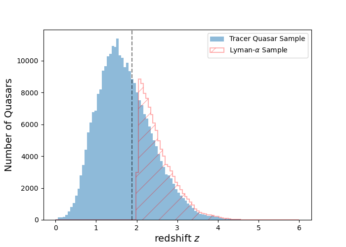
(a) Redshift distribution for the tracer quasar sample (without BALs) used in this paper. The red hatched histogram represents the Lyman-$\alpha$ forest sample. The dashed grey line represents the lower bound on the tracer quasar sample, $z=1.88$.

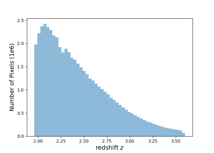
(b) Redshift distribution of Lyman-$\alpha$ forest pixels output during the continuum fitting process for the baseline analysis.

Figure 1: Redshift and Lyman-$\alpha$ forest pixel distributions for the tracer quasar and Lyman-$\alpha$ forest samples used in this work.

To finalize our catalog, we select only the objects that were targeted as quasars, using the classifications provided by the DESI target-selection pipeline [33]. Some of these objects were observed multiple times during EDR and M2 and therefore have multiple entries, but we want to keep only one observation per object in the quasar catalog. To select the best observation for the duplicated quasars, we first remove those that have a redshift warning flags set (i.e, those with a bad fit). If there are still repeat observations of the same quasar at this point, we select the observation with the highest TSNR2_LYA value. TSNR2_LYA, which is defined in section 4.14 of [23], is a measure related to the signal to noise ratio in the blue part of spectra for a given observation. We also remove any BAL quasars that were identified by the BALFinder [34] as having their absorption index (AI) > 0.

After these cuts, a total of 290,506 quasars are present in the quasar catalog. However, only the 106,861 quasars with redshift z > 1.88 will be included in the cross-correlation discussed in section 3.2. We refer to these quasars as tracer quasars or the tracer quasar catalog. Figure 1(a) shows the redshift distribution of the entire quasar sample with the dashed grey line representing this cutoff for the tracer quasar sample. The red hatched histogram shows the redshift distribution for the Lyman-$\alpha$ sample discussed in the next section.

2.2 Lyman-$\alpha$ Forest Sample

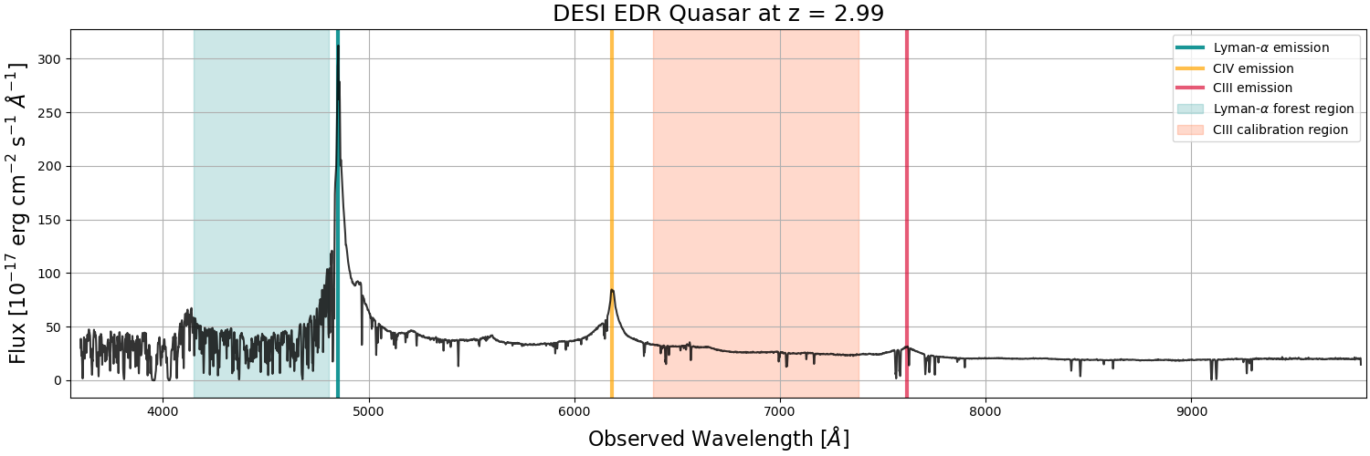
Figure 2: An example of a quasar spectrum from DESI EDR at redshift 2.99 and TARGETID = 39633362754732929. The observed Lyman-$\alpha$ emission line is shown in teal, CIV in orange and CIII] in red. The orange shaded region is the CIII calibration region, and the Lyman-$\alpha$ forest region is shaded in teal, both are used in the continuum fitting process in section 3.1. Redward of the Lyman-$\alpha$ emission are some absorption lines, likely from various metals.

We use the same Lyman-$\alpha$ forest sample as described in [35]. We will briefly describe the sample here, but refer the reader to [35] for a more detailed description.

We define the Lyman-$\alpha$ forest as the region between the Lyman-$\beta$ and Lyman-$\alpha$ emission lines at 1025.7 Å and 1215.67 Å, respectively. To reduce any contamination from the wings of those emission lines, we reduce the rest-frame wavelength range of all the Lyman-$\alpha$ forests to 1040 Å < $\lambda$ < 1205 Å. An example quasar spectrum highlighting the Lyman-$\alpha$ forest is shown in figure 2. Other features highlighted are the CIV and semi-forbidden CIII emission lines. The region between these lines shaded in orange is used during the calibration step of the continuum fitting process discussed in section 3.1 and in [35].

The Lyman-$\alpha$ forest sample is created from the same quasar catalog described in section 2.1, but the BAL quasars are not excluded. We set a limit on the observed wavelength range of the Lyman-$\alpha$ forest between 3600 Å and 5772 Å. The lower limit is set to the lowest wavelength measured by the blue DESI spectrographs [23] and corresponds to a minimum Lyman-$\alpha$ pixel redshift of $z=1.96$, meaning the lowest redshift a quasar can have is $z=2.02$. The upper limit is set by the small number of high redshift quasars in EDR+M2. This limit corresponds to a maximum quasar redshift of $z$ = 4.29 (with a corresponding maximum Lyman-$\alpha$ pixel redshift of $z=3.75$).

With these redshift cuts, there are 109,900 valid Lyman-$\alpha$ forests from the quasar catalog. Prior to fitting the continuum (described in section 3.1), we first mask regions of the spectra that are contaminated. This contamination can come from sky lines, galactic absorption, BALs, and Damped Lyman Alpha (DLA) regions. We mask any DLA regions identified with the DLAFinder [36] and BAL regions identified with the BALFinder [34] of the quasar spectra. For the sky lines and galactic absorption, we mask four areas of the spectra: sky lines from [5570.5, 5586.7] Å; and the Ca H, and K lines from the Milky Way from [3967.3, 3971.0] Å and [3933.0, 3935.8] Å, respectively. We also perform a calibration using the CIII between 1600 < $\lambda_{\text{RF}}$ [Å] < 1850, which is shaded in orange in figure 2. This calibration step follows the same process described in section 3.1 and in [35]. We require each forest to have a minimum length of 40 Å. Forests that are too short (don’t have enough pixels), have low signal (< 0), or have problems fitting the continuum (negative continuum) will be rejected during the calibration and continuum fitting process (section 3.1). After these rejections, the final Lyman-$\alpha$ sample has 88,511 forests. Figure 1(b) shows the redshift distribution of Lyman-$\alpha$ pixels in the sample.

3 Method

We measure and model the cross-correlation of the Lyman-$\alpha$ forest with quasars following the method in [14, 8] and for the continuum fitting process we follow the method in [35]. We will briefly discuss the method for this analysis starting with the continuum fitting in section 3.1, calculating the cross-correlation function in section 3.2, the distortion and covariance matrices in section 3.3, and the model in section 3.4. We perform the calculations in sections 3.1-3.3 using picca, and we perform the modeling in section 3.4 using vega.

3.1 Measuring the Flux Transmission Field

We follow the method in [35] to measure the flux transmission field for the Lyman-$\alpha$ sample. We will briefly describe the method here but refer the reader to [35] for a more detailed description.

In this work, we adopt the same 0.8 Å linear pixel size used by the DESI spectroscopic pipeline [23] and other Lyman-$\alpha$ forest analyses using DESI EDR+M2 data [14, 35]. Previous analyses in eBOSS used logarithmic pixels [8]. We follow the method described in [35].

For each forest in each line of sight, $q$, we calculate the flux transmission field $\delta_{\text{q}}$ as a function of observed wavelength:

$$\delta_{\text{q}}(\lambda)=\frac{f_{\text{q}}(\lambda)}{\overline{F}(\lambda)C_{\text{q}}(\lambda)}-1.$$ (3.1)

Here, $f_{\text{q}}(\lambda)$ is the observed flux, $C_{\text{q}}(\lambda)$ is the unabsorbed quasar continuum, and $\overline{F}(\lambda)$ is the mean transmitted flux at a specific wavelength. To measure each delta field, we estimate the mean expected flux, $\overline{F}(\lambda)C_{\text{q}}(\lambda)$, which is the product of the terms in the denominator in eq. 3.1. We assume it can be expressed according to:

$$\overline{F}(\lambda)C_{\text{q}}(\lambda)=\overline{C}(\lambda_{\text{RF}})\left(a_{\text{q}}+b_{\text{q}}\frac{\Lambda-\Lambda_{\text{min}}}{\Lambda_{\text{max}}-\Lambda_{\text{min}}}\right),$$ (3.2)

where $\Lambda\equiv\log\lambda$, $\overline{C}(\lambda_{\text{RF}})$ is the estimate of the mean continuum for the considered quasar sample, and $a_{\text{q}}$, $b_{\text{q}}$ are per-quasar parameters.

The estimated variance of the flux $\sigma_{\text{q}}^{2}$ depends on the noise from the DESI spectroscopic pipeline and the intrinsic variance of the Lyman-$\alpha$ forest ($\sigma_{\text{LSS}}^{2}$) and we model it as

$$\frac{\sigma_{\text{q}}^{2}(\lambda)}{(\overline{F}C_{\text{q}}(\lambda))^{2}}=\eta(\lambda)\tilde{\sigma}_{\text{pip,q}}^{2}+\sigma_{\text{LSS}}^{2},$$ (3.3)

where $\tilde{\sigma}_{\text{pip,q}}=\sigma_{\text{pip,q}}/\overline{F}C_{\text{q}}(\lambda)$ and $\sigma_{\text{pip,q}}$ is the spectroscopic pipeline estimate of the flux uncertainties. It is further modified by the correction, $\eta(\lambda)$, which accounts for inaccuracies in the spectroscopic pipeline noise estimation. In DESI $\eta(\lambda)$ ranges between 0.97 and 1.05 between 3600 Å and 5772 Å, respectively, and is generally close to 1 due to first performing a calibration using the CIII region. The mean continuum $\overline{C}(\lambda_{\text{RF}})$, the function $\eta(\lambda)$, $\sigma_{\text{LSS}}(\lambda)$, and the quasar parameters, $a_{\text{q}}$ and $b_{\text{q}}$, are fit in an iterative process and stable values are obtained after about 5 iterations.

3.2 The Lyman-$\alpha$ Forest-Quasar Cross-Correlation

In this work we study the Lyman-$\alpha$ forest-quasar cross-correlation function. We require the use of the Lyman-$\alpha$ auto-correlation function to constrain some of the fit parameters (discussed in section 5). We use the Lyman-$\alpha$ forest auto-correlation results from [14] and, when necessary (in sections 4 and 5.3), run the auto-correlation following the method in [14]. The results of the cross-correlation are presented in section 5.1.

The separation between two tracers is determined both parallel and perpendicular to the line of sight, with $\vec{r}$ = ($r_{\parallel}$, $r_{\perp}$). For two tracers i and j with redshift $z_{\text{i}}$ and $z_{\text{j}}$, that are offset by an observed opening angle $\Delta\theta$, the comoving separation can be computed as

$$r_{\parallel}=\left[D_{\text{c}}(z_{\text{i}})-D_{\text{c}}(z_{\text{j}})\right]\cos{\left(\frac{\Delta\theta}{2}\right)},$$ (3.4a)

$$r_{\perp}=\left[D_{\text{m}}(z_{\text{i}})+D_{\text{m}}(z_{\text{j}})\right]\sin{\left(\frac{\Delta\theta}{2}\right)},$$ (3.4b)

where $D_{\text{c}}(z)=c\int_{0}^{z}dz/H(z)$ is the comoving distance, $D_{\text{m}}$ is the angular comoving distance, and $H(z)$ is the Hubble function. To use the comoving distance we have to assume a fiducial cosmology and we adopt the flat $\Lambda$CDM cosmology of Planck Collaboration et al. (2018) [37]. With this cosmology we have $D_{\text{c}}=D_{\text{m}}$. In the above equations, the two tracers are either two Lyman-$\alpha$ pixels for the auto-correlation or a Lyman-$\alpha$ pixel and a quasar for the cross-correlation. The redshift of a Lyman-$\alpha$ pixel is calculated as $z_{\text{i}}=\lambda_{\text{obs}}/\lambda_{\text{Ly$\alpha$}}-1$, where $\lambda_{\text{Ly$\alpha$}}=1215.67$ Å and the quasar redshift is given from the tracer quasar catalog described in section 2.1.

The cross-correlation of the Lyman-$\alpha$ forest with quasars is defined as

$$\xi(\vec{r}_{\text{A}})=\langle\delta_{\text{Q}}(\vec{x})\delta(\vec{x}+\vec{r}_{\text{A}})\rangle\approx\langle\delta(\vec{x}_{\text{Q}}+\vec{r}_{\text{A}})\rangle,$$ (3.5)

where $\delta_{\text{Q}}(\vec{x})$ is the fluctuation of the number density in quasars, and $\vec{r}=(r_{\parallel},r_{\perp})$ (with $r^{2}=r_{\parallel}^{2}+r_{\perp}^{2}$) for bin A. If we assume that quasars are shot-noise dominated, then the cross-correlation is just the average Lyman-$\alpha$ transmission around quasars at $\vec{x}_{\text{Q}}$ [38].

For the Lyman-$\alpha$-quasar cross-correlation we use the same estimator as previous studies [8, 14, 39]:

$$\xi_{\text{A}}=\frac{\sum_{\text{(i,j)$\in$A}}w_{\text{i}}w_{\text{j}}\delta_{\text{i}}}{\sum_{\text{(i,j)$\in$A}}w_{\text{i}}w_{\text{j}}},$$ (3.6)

where $i$ indexes a Lyman-$\alpha$ pixel and $j$ a quasar, and $\delta_{\text{i}}$ is the flux transmission for the Lyman-$\alpha$ pixel defined in eq. 3.1. The weights $w$ are defined in [14] and proportional to $(1+z)^{\gamma-1}$, where $\gamma=1.44$ for quasars and 2.9 for a Lyman-$\alpha$ pixel. The sums are over all quasar-pixel pairs with separations that are within the bounds of bin A, with the exception of Lyman-$\alpha$ pixels from their own background quasar which are excluded. The bounds of bin A are defined in comoving coordinates and are determined based on the selected bin width.

The correlation is binned along and across the line of sight, but the cross-correlation itself is not symmetric (i.e, you can’t swap indices $i$ and $j$ for $\delta_{i}$ in eq. 3.6). We define a positive separation along the line of sight when the quasar is in front of the Lyman-$\alpha$ pixel ($z_{qso}<z_{Ly\alpha}$) and likewise define a negative separation along the line of sight when the quasar is behind the Lyman-$\alpha$ pixel ($z_{qso}>z_{Ly\alpha}$). This asymmetry in the cross-correlation is what allows us to study systematic quasar redshift errors.

In this work we are studying small-scale effects on the cross-correlation, so we do not need to extend to large values of $r_{\parallel}$ and $r_{\perp}$, unlike the studies of BAO and the full-scale correlations in [14, 8]. We instead use a maximum separation of $80\,h^{-1}\,\mathrm{Mpc}$ in both $r_{\parallel}$ and $r_{\perp}$. For the cross-correlation, this corresponds to a minimum tracer quasar redshift of $z=1.88$ given the minimum Lyman-$\alpha$ pixel redshift of $z=1.96$ given in section 2.2.

Since our maximum separation in this study is $80\,h^{-1}\,\mathrm{Mpc}$, for the cross-correlation we restrict $r_{\parallel}$ $\in[-80,80]$ $h^{-1}$ Mpc and $r_{\perp}$ $\in[0,80]$ $h^{-1}$ Mpc. Previous measurements of 3D correlations to study BAO with eBOSS or DESI [14, 8] used a bin width of $4\,h^{-1}\,\mathrm{Mpc}$. Here, the focus of this paper is to measure a small-scale effect, we use a bin width of $1\,h^{-1}\,\mathrm{Mpc}$, along both transverse and longitudinal separations. This gives us 80 bins across the line of sight, 160 bins along the line of sight, and N = 80 $\times$ 160 = 12800 bins in total. We validate our choice to use a $1\,h^{-1}\,\mathrm{Mpc}$ bin width with mock data in section 4.

3.3 The Distortion and Covariance Matrices

We follow the same method as in [14] to estimate the covariance matrix for the cross-correlation. The covariance matrix is estimated by splitting the sky into $s$ regions (according to HEALPix pixels) and then computing their weighted covariance. Assuming that correlations between regions are negligible, the covariance is written as

$$C_{\text{AB}}=\frac{1}{W_{\text{A}}W_{\text{B}}}\sum_{\text{s}}W^{\text{s}}_{\text{A}}W^{\text{s}}_{\text{B}}[\xi^{\text{s}}_{\text{A}}\xi^{\text{s}}_{\text{B}}-\xi_{\text{A}}\xi_{\text{B}}],$$ (3.7)

where A and B are two different bins of the correlation function $\xi$, $W=\sum_{\text{s}}W^{\text{s}}$, $W^{\text{s}}$ is the summed weight for one of the regions $s$, and $\xi_{\text{A}}=\sum_{\text{s}}W_{\text{A}}^{\text{s}}\xi_{\text{A}}^{\text{s}}/W_{\text{A}}$.

The covariance matrix is dominated by the diagonal elements (the variance) of the matrix. The estimates of off-diagonal elements are noisy, so they are modeled as a function of the difference of separation along the line of sight ($\Delta r_{\parallel}=|r^{\text{A}}_{\parallel}-r^{\text{B}}_{\parallel}|$) and across the line of sight ($\Delta r_{\perp}=|r^{\text{A}}_{\perp}-r^{\text{B}}_{\perp}|$) and then smoothed [8]. Correlation coefficients that have the same $\Delta r_{\parallel},\Delta r_{\perp}$ are averaged.

Using the Lyman-$\alpha$ forest when estimating the quasar continuum biases the estimates of the delta field in eq. 3.1 because the measured delta for a given pixel is a combination of the absorption signals located at other pixels. This produces a distortion in the correlation functions that occurs throughout, but mainly appear for small $r_{\perp}$. The biases arise because

1. fitting the quasar parameters $a_{\text{q}}$ and $b_{\text{q}}$ biases the mean $\delta_{\text{q}}$ toward 0, and

2. fitting the mean transmitted flux, $\overline{F}$, biases the mean $\delta$ at each observed wavelength, $\overline{\delta(\lambda)}$, toward 0.

These effects can be modeled by transformations to $\delta_{\text{q}}(\lambda)$. With the assumption that these transformations to $\delta_{\text{q}}$ are linear, the correlation function is distorted by a distortion matrix, $D_{\text{AA'}}$, such that

$$\xi^{\text{distorted}}_{\text{A}}=\sum_{\text{A'}}D_{\text{AA'}}\xi^{\text{true}}_{\text{A'}}.$$ (3.8)

For the cross-correlation, the distortion matrix is calculated as

$$D_{\text{AA'}}^{\text{cross}}=\frac{\sum_{\text{(i,k)$\in$A}}w_{\text{i}}\sum_{\text{(j,k)$\in$A'}}\eta_{\text{ij}}}{\sum_{\text{(i,k)$\in$A}}w_{\text{i}}},$$ (3.9)

where $\eta$ is the projection due to the distortion that occurs during the continuum fitting process and is defined in equation 3.3 of [14], and the weights $w$ are defined in eq. 3.6.

When fitting the data, (described in section 3.4), the physical model of the correlation function is multiplied by the distortion matrix.

3.4 The Model of the Lyman-$\alpha$ Forest-Quasar Cross-correlation

This section presents the theoretical model for the auto- and cross-correlations. Though this work focuses on the cross-correlation, the auto-correlation is necessary to include during the fitting process as it helps break degeneracies between parameters.

In this model, the expected measured (distorted) cross-correlation in the ($r_{\parallel}$, $r_{\perp}$) bin $A$ is related to the theoretical (true) correlation by the distortion matrix as shown in eq. 3.8. The theoretical cross-correlation, $\xi^{\text{qf,th}}$, can be broken down into the sum of its components:

$$\xi^{\text{qf,th}}=\xi^{\text{Ly$\alpha\times$QSO}}+\sum_{\text{a}}\xi^{\text{QSO$\times$a}}+\xi^{\text{TP}}.$$ (3.10)

Here, the first term gives the contribution from the cross-correlation between the Lyman-$\alpha$ forest and quasars, the second term gives the contribution from the cross-correlation between quasars and other absorbers, like metals and high column density systems (HCDs), in the Lyman-$\alpha$ region, and the last term gives the contributions from the transverse proximity (TP) effect, which is the effect of radiation from the quasar on the nearby surrounding gas. We describe these terms in depth throughout this section and the parameters of this model are described in table 5.

The Lyman-$\alpha$-QSO contribution to the correlation function is derived from the Fourier transform of the tracer biased power spectrum, $P(\textbf{k},z)$, which is written as

$$P(\textbf{k},z)=b_{\text{i}}(z)b_{\text{j}}(z)(1+\beta_{\text{i}}\mu_{\text{k}}^{2})(1+\beta_{\text{j}}\mu_{\text{k}}^{2})P_{\text{QL}}(\textbf{k},z)F_{\text{NL}}(\textbf{k})G(\textbf{k}),$$ (3.11)

where k is the wavenumber with modulus $k$ and $\mu_{\text{k}}=k_{\parallel}/k$. The bias and linear redshift-space distortion parameters, $b_{\text{i,j}}(z)$ and $\beta_{\text{i,j}}$, are for tracer $i$ or $j$. $G$ is a correction that accounts for the averaging of the correlation function binning and $F_{\text{NL}}$ accounts for the non-linear effects on small scales (large k). $P_{\text{QL}}$ is the quasi-linear matter power spectrum defined in eq. 3.16. For the auto-correlation, $i=j$ and the only tracer is Lyman-$\alpha$ absorption. In this work, we are concerned with the cross-correlation, $i\neq j$ and the two tracers are Lyman-$\alpha$ absorption and quasars.

In eq. 3.11, the bias $b$ and redshift-space distortion $\beta$ parameters for each tracer $i,j$ appear with the standard Kaiser factor: $b_{\text{i,j}}(z)(1+\beta_{\text{i,j}}\mu_{\text{k}}^{2})$ [40]. The fit of the cross-correlation is only sensitive to the product of the quasar and Lyman-$\alpha$ biases. The quasar bias $b_{\text{q}}$ is redshift dependent and is given by

$$b_{\text{q}}(z)=b_{\text{q}}(z_{\text{eff}})\left(\frac{1+z}{1+z_{\text{eff}}}\right)^{\gamma_{\text{q}}},$$ (3.12)

where $z_{\text{eff}}$ is the effective redshift of the sample and $\gamma_{\text{q}}$ = 1.44 [41]. Following the analysis of [14] we allow $b_{\text{q}}$ to remain free in the fit. On the other hand, the quasar redshift-space distortion (RSD) parameter, $\beta_{\text{q}}$, is not a free parameter. It is related to the quasar bias $b_{\text{q}}$ by:

$$\beta_{\text{q}}=\frac{f}{b_{\text{q}}},$$ (3.13)

where $f=0.9703$ is the linear growth rate of structure in our fiducial cosmology. We then derive the value of $\beta_{\text{q}}$ from the result of $b_{\text{q}}$.

We assume that the Lyman-$\alpha$ bias parameter, $b_{\text{Ly$\alpha$}}$, is redshift dependent but use the approximation that the Lyman-$\alpha$ RSD parameter, $\beta_{\text{Ly$\alpha$}}$, is redshift independent. Following [14], $b_{\text{Ly$\alpha$}}$ is given by

$$b_{\text{Ly$\alpha$}}(z)=b_{\text{Ly$\alpha$}}(z_{\text{eff}})\left(\frac{1+z}{1+z_{\text{eff}}}\right)^{\gamma_{\text{Ly$\alpha$}}},$$ (3.14)

with $\gamma_{\text{Ly$\alpha$}}$ = 2.9 [42]. We allow $b_{\text{Ly$\alpha$}}$ and $\beta_{\text{Ly$\alpha$}}$ to remain free in the fit.

The Lyman-$\alpha$ absorption contains contributions from both the inter-galactic medium (IGM) and high-column-density (HCD) systems. HCD absorbers, such as Damped Lyman Alpha, trace the underlying density field. When these HCD systems are correctly identified and the appropriate parts of the absorption region are properly masked and modeled, they will have no effect on the measured correlation functions. However, if these systems are left unidentified, they will affect the measured correlation function as a broadening/smearing in the radial direction. Following the method in [43], this effect introduces a $k_{\parallel}$ dependence to the effective bias and can be modeled as

$$\begin{split}b^{\prime}_{\text{Ly}\alpha}&=b_{\text{Ly}\alpha}+b_{\text{HCD}}F_{\text{HCD}}(k_{\parallel}),\\ b^{\prime}_{\text{Ly}\alpha}\beta^{\prime}_{\text{Ly}\alpha}&=b_{\text{Ly}\alpha}\beta_{\text{Ly}\alpha}+b_{\text{HCD}}\beta_{\text{HCD}}F_{\text{HCD}}(k_{\parallel}),\end{split}$$ (3.15)

where $(b_{\text{Ly}\alpha},\beta_{\text{Ly}\alpha})$ and $(b_{\text{HCD}},\beta_{\text{HCD}})$ are the bias and redshift space distortion parameters associated with the IGM and HCD systems. Following [8], we use $F_{\text{HCD}}=\exp(-L_{\text{HCD}}k_{\parallel})$, which is approximated from the results in [44]. $L_{\text{HCD}}$ is the length scale for unmasked HCDs, and is degenerate with other parameters. For this work, we fix $L_{\text{HCD}}=$ $10\,h^{-1}\,\mathrm{Mpc}$ and allow $b_{\text{HCD}}$ to be free in the fit. We fix $\beta_{\text{HCD}}=0.5$.

While this work focuses on comoving separations smaller than the BAO scale, for consistency with other analyses [14, 45], we model the quasi-linear matter power spectrum, $P_{\text{QL}}(\textbf{k},z)$, as the sum of a smooth and peak components with an empirical anisotropic damping applied to the BAO peak component:

$$P_{\text{QL}}(\textbf{k},z)=P_{\text{sm}}(k,z)+A_{\text{peak}}\exp{\left[-\frac{k^{2}_{\parallel}\Sigma^{2}_{\parallel}+k^{2}_{\perp}\Sigma^{2}_{\perp}}{2}\right]}P_{\text{peak}}(k,z).$$ (3.16)

$P_{\text{sm}}$ in eq. 3.16 is derived from the linear power spectrum $P_{\text{L}}(k,z)$ via the side-band technique described in [46]. The redshift dependent linear power spectrum, $P_{\text{L}}$, is derived from CAMB [47], and we then define $P_{\text{peak}}=P_{\text{L}}-P_{\text{sm}}$. The BAO peak is affected by non-linear broadening [48] and is corrected for by introducing the parameters $(\Sigma_{\parallel},\Sigma_{\perp})$. $\Sigma_{\parallel}$ is related to $\Sigma_{\perp}$ and the growth rate such that

$$\frac{\Sigma_{\parallel}}{\Sigma_{\perp}}=1+f,$$ (3.17)

where $f=0.9703$ is the linear growth rate of structure in our fiducial cosmology. Given that we do not fit the BAO peak in this work, we fix ($A_{\text{peak}},~{}\Sigma_{\parallel},~{}\Sigma_{\perp}$) = (1, $6.37\,h^{-1}\,\mathrm{Mpc}$, $3.24\,h^{-1}\,\mathrm{Mpc}$) [14].

$F_{\text{NL}}$ in equation 3.11 corrects for additional effects at small scales. In the auto-correlation these are thermal broadening, peculiar velocities, and nonlinear growth structure, parameterized according to equation 3.6 in [49]. For the cross-correlation the most important small-scale correction is due to quasar velocities and the precision of quasar redshift measurements. Following [14, 50], we model this using the Lorentz-damping form:

$$F_{\text{NL}}^{\text{cross}}(k_{\parallel})=\frac{1}{\sqrt{1+(k_{\parallel}\sigma_{\text{v}})^{2}}},$$ (3.18)

where $\sigma_{\text{v}}$ is a free parameter that describes the precision of quasar redshift measurements. Alternative models for $F_{\text{NL}}$ use a Gaussian form.

The last term in eq. 3.11, $G(\textbf{k})$, accounts for the effects of the binning of the correlation function on the $(r_{\parallel},r_{\perp})$ separation grid. Assuming the distribution in each bin is homogeneous, and following the method used in [51],

$$G(\textbf{k})=\text{sinc}\left(\frac{R_{\parallel}k_{\parallel}}{2}\right)\text{sinc}\left(\frac{R_{\perp}k_{\perp}}{2}\right),$$ (3.19)

where $R_{\parallel}$ and $R_{\perp}$ are the scales of the smoothing, i.e, are the radial and transverse widths of the bins, respectively. In this work we focus on bin widths of $1\,h^{-1}\,\mathrm{Mpc}$ for both $R_{\parallel}$ and $R_{\perp}$, but validate the choice between $1\,h^{-1}\,\mathrm{Mpc}$ and $4\,h^{-1}\,\mathrm{Mpc}$ in section 4.

The next component that contributes to the model cross-correlation in eq. 3.10 is the sum over the non-Lyman-$\alpha$ absorbers, or metals. The power spectrum for the cross-correlation with metals has the same form as that used for the Lyman-$\alpha$-quasar cross-correlation, though it is simplified by neglecting the effect of HCDs. Because there is little absorption by metals, it is further simplified by not separating the smooth and peak components. It is however, more complicated due to the fact that the ($r_{\parallel}$, $r_{\perp}$) bins in the correlation correspond to an observed $(\Delta\theta,\Delta\lambda)$ calculated assuming that the absorption is due to the Lyman-$\alpha$ transition.

This causes a shift in the model correlation function, and the contribution of each absorber is maximized in the ($r_{\parallel}$, $r_{\perp}$) bin that corresponds to vanishing physical separation. For Lyman-$\alpha$ absorption this corresponds to ($r_{\parallel}$, $r_{\perp}$) = (0,0). For the other absorbers, this maximum occurs at $r_{\perp}$ = 0 and $r_{\parallel}\approx\frac{c}{H(z)}(1+z)(\lambda_{\text{m}}-\lambda_{\text{Ly}\alpha})/\overline{\lambda}$, where $\overline{\lambda}$ is the mean value between the $\text{Ly}\alpha$ and metal absorption [14]. The values of the $r_{\parallel}$ separations for the metal absorbers considered in this work are given in table 1.

Transition	$\lambda_{\text{m}}$ [Å]	$\lambda_{\text{m}}/\lambda_{\text{Ly}\alpha}$	Lyman-$\alpha$-m $r_{\parallel}$ [ $h^{-1}$ Mpc ]
SiII(1260)	1260.4	1.036	+104
SiIII(1207)	1206.5	0.992	-22
SiII(1193)	1193.3	0.981	-55
SiII(1190)	1190.4	0.979	-62

Table 1: Metal transitions seen in the IGM and that are also present in the Lyman-$\alpha$ forest-quasar cross correlation for $r_{\parallel}\in[-80,80]$  $h^{-1}$ Mpc. The second column gives the rest-frame wavelength of the transition in Angstroms. The third column is the ratio between the wavelengths of the metal transition and the Lyman-$\alpha$ transition (1215.67 Å). The last column gives the error in comoving distance when a metal absorption is incorrectly assumed to be Lyman-$\alpha$ absorption at $z=0$.

The shifted-model correlation function is calculated with respect to the unshifted-model correlation function, $\xi^{mn}$, for each absorber pair $(m,n)$ by introducing a metal matrix $M_{\text{AB}}$ as in [52]:

$$\xi^{\text{mn}}_{\text{A}}\longrightarrow\sum_{\text{B}}M_{\text{AB}}\xi^{\text{mn}}(r_{\parallel}(B),r_{\perp}(B)),$$ (3.20)

where $M_{\text{AB}}$, the metal matrix, is defined as

$$M_{\text{AB}}=\frac{1}{W_{\text{A}}}\sum_{\text{(m,n)$\in$A,(m,n)$\in$B}}w_{\text{m}}w_{\text{n}}.$$ (3.21)

Here, $W_{\text{A}}=\sum_{\text{(m,n)$\in$A}}w_{\text{m}}w_{\text{n}}$ and $w_{\text{m}},w_{\text{n}}$ are the weights for each absorber and are redshift dependent such that $w\propto(1+z)^{\gamma}$. $(m,n)\in A$ refers to separations calculated using the reconstructed redshift of the absorber pair and $(m,n)\in B$ refers to separations computed using the redshifts $z_{\text{m}}$ and $z_{\text{n}}$ of the absorber pair $(m,n)$.

In the fits to the data each metal species has its own individual bias parameters $(b,\beta)$. Since the correlations are only visible in ($r_{\parallel}$, $r_{\perp}$) bins that correspond to small physical separations and the amplitudes for the SiII and SiIII metal species are determined by the excess correlations, we do not have enough signal to determine the $(b,\beta)$ parameters separately. As in previous works ([8, 50]), we fix $\beta=0.5$ for all metal species. Since we are using the auto-correlation from [14] we include correlations from the four metal species given in table 1 in the correlations.

The last term in eq. 3.10 is due to the transverse proximity effect. In the area surrounding a quasar, there is significantly less Lyman-$\alpha$ absorption because the radiation emitted from the quasar dominates over the UV background and increases the ionization fraction of the surrounding gas, thus making it more transparent to Lyman-$\alpha$ photons. The Lyman-$\alpha$ absorption of a background quasar will decrease in strength at the redshift of the foreground quasar when the Lyman-$\alpha$ forest is close to the quasar line of sight. This will therefore affect the correlation between quasars and the Lyman-$\alpha$ forest. As in [14], we model this effect in the correlation with

$$\xi^{\text{TP}}=\frac{\xi^{\text{TP}}_{0}}{r^{2}}\exp{\left[\frac{-r}{\lambda_{\text{UV}}}\right]},$$ (3.22)

where $r$ is the comoving separation in units of  $h^{-1}$ Mpc, $\lambda_{\text{UV}}=$$300\,h^{-1}\,\mathrm{Mpc}$ [53], and $\xi_{0}^{TP}$ is an amplitude that will be fit.

Systematic errors on the measurement of the quasar redshift can cause a shift in the model estimation of the correlation function in $r_{\parallel}$. To account for this, we allow for a shift of the absorber-quasar separation in the $r_{\parallel}$ direction

$$\Delta r_{\parallel}=r_{\parallel,\text{true}}-r_{\parallel,\text{measured}}.$$ (3.23)

The shift is mostly due to systematic quasar redshift errors. However, any asymmetries in $r_{\parallel}$ will also affect $\Delta r_{\parallel}$. The model of the cross-correlation function is not symmetric about $r_{\parallel}$ due to the contribution of metal absorptions and the variation of mean redshift with $r_{\parallel}$. The continuum-fitting distortion also introduces an asymmetry in $r_{\parallel}$. [54] has showed that while $\Delta r_{\parallel}$ is sensitive to relativistic effects, they are small. We do not model any relativistic effects in this work as [55] showed that they are partially degenerate with $\Delta r_{\parallel}$.

4 Validation with Mock Data

To ensure that the choice of bin width does not introduce any biases to our analysis, and especially to the two redshift error parameters $\Delta r_{\parallel}$ and $\sigma_{\text{v}}$, we run our tests using mock data for three different cross-correlation bin widths: $1\,h^{-1}\,\mathrm{Mpc}$, $2\,h^{-1}\,\mathrm{Mpc}$, and $4\,h^{-1}\,\mathrm{Mpc}$. We follow the same method described in section 3, however we do not need to perform the calibration step on mock data (section 3.1). For the cross-correlation, we still restrict $r_{\parallel}$, $r_{\perp}$ $\in$ $[-80,80]\,h^{-1}\,\mathrm{Mpc}$. For the $2\,h^{-1}\,\mathrm{Mpc}$ bin width, this gives 80 bins along the line of sight, 40 bins across the line of sight and N = 3,200 bins in total. For the $4\,h^{-1}\,\mathrm{Mpc}$ bin width, this gives 40 bins along the line of sight, 20 bins across the line of sight, and N = 800 bins in total. Since the auto-correlation doesn’t help to constrain redshift errors we choose to follow the setup from [14] as we use the auto-correlations from [14] in section 5. The free and fixed parameters are described in table 5 in appendix A.

In this work we use the mocks described in [56]. There are 10 realizations of Saclay [57] mocks that contain signal from the Lyman-$\alpha$ forest as well as contamination from DLAs, BALs, and metals, which most closely resembles the data from EDR+M2. Like in our baseline analysis, we mask the BAL and DLA regions during the continuum fitting process, and we remove any BAL quasars from the tracer quasar catalog. Each mock has approximately 118,000 objects in the catalog after BAL removal.

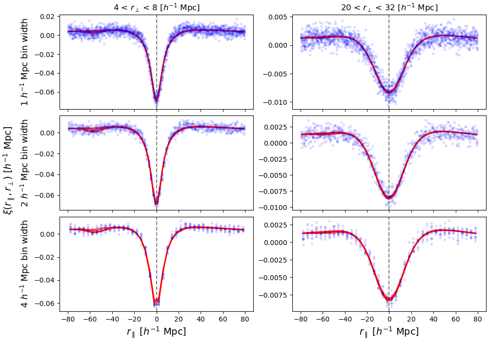
Figure 3: Results for 10 different realizations of mocks comparing the correlation function to the best-fit model. The data (blue points) and model (red lines) are averaged across $r_{\perp}$ $\in$ [4,8] (left column) and $r_{\perp}$ $\in$ [20,32] (right column). We compare the different bin widths studied in this analysis with $1\,h^{-1}\,\mathrm{Mpc}$ on the top row, $2\,h^{-1}\,\mathrm{Mpc}$ in the middle, and $4\,h^{-1}\,\mathrm{Mpc}$ on the bottom row. The dashed grey line represents $r_{\parallel}$ = 0.

We present the results of the cross-correlation and best-fit model for each mock for two $r_{\perp}$ slices ($r_{\perp}$ $\in$ [4,8] $h^{-1}$ Mpc and $r_{\perp}$ $\in$ [20,32] $h^{-1}$ Mpc) in figure 3. The data and model are averaged across the $r_{\perp}$ slices for each mock. There are 4 times fewer points in the bottom row of figure 3 compared to the top row due to the bin width being 4 times larger. There is a bump in the correlations around $r_{\parallel}$ $\approx$ $-60\,h^{-1}\,\mathrm{Mpc}$ that likely corresponds to the effects from SiII $\lambda$1193 and $\lambda$1190 metal lines, which appear in the correlations as given in table 1. This bump is not as prominent in the larger $r_{\perp}$ slices as the metals have the largest effect at $r_{\perp}$ = 0. There does not appear to be a shift from 0 in $r_{\parallel}$, as the center of the peaks corresponds with the dashed grey line at $r_{\parallel}$ = 0.

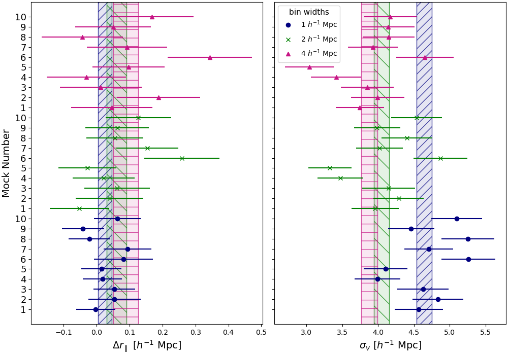
Figure 4: Results for 10 different realizations of mocks comparing the redshift error parameters, $\Delta r_{\parallel}$ (left) and $\sigma_{\text{v}}$ (right) for the three different bin widths being studied: $1\,h^{-1}\,\mathrm{Mpc}$ (blue dots), $2\,h^{-1}\,\mathrm{Mpc}$ (green x’s), and $4\,h^{-1}\,\mathrm{Mpc}$ (pink triangles). The hatched shaded regions are showing the weighted average value + error for all 10 mocks.

The two parameters of interest in our model that describe redshift errors are $\Delta r_{\parallel}$ and $\sigma_{\text{v}}$. $\Delta r_{\parallel}$ describes the shift of the cross-correlation due to systematic redshift errors in quasars along the $r_{\parallel}$ direction. $\sigma_{\text{v}}$ measures the radial velocity smearing due to random redshift errors and non-linear velocities. This is often represented as the rms velocity dispersion from a Lorentz damping factor [58, 50]. Here, a smaller value for $\sigma_{\text{v}}$ means the redshift measurements are more accurate.

The mocks studied here do not have any systematic errors added to the quasar redshift so we expect $\Delta r_{\parallel}$ $\sim 0$. The true value of $\sigma_{\text{v}}$ is known and we do not expect it to be 0, as the mocks include non-linear effects. The results for these parameters for each mock and each bin width tested are shown in figure 4. The weighted average across all mocks is shown by the hatched shaded regions. For the $1\,h^{-1}\,\mathrm{Mpc}$ bin width: $\Delta r_{\parallel}$ = $0.039\pm 0.021$ $h^{-1}$ Mpc and $\sigma_{\text{v}}=4.64\pm 0.11$ $h^{-1}$ Mpc. For the $2\,h^{-1}\,\mathrm{Mpc}$ bin width: $\Delta r_{\parallel}$ = $0.079\pm 0.030$ $h^{-1}$ Mpc and $\sigma_{\text{v}}=4.05\pm 0.11$ $h^{-1}$ Mpc. For the $4\,h^{-1}\,\mathrm{Mpc}$ bin width: $\Delta r_{\parallel}$ = $0.10\pm 0.04$ $h^{-1}$ Mpc and $\sigma_{\text{v}}=3.88\pm 0.11$ $h^{-1}$ Mpc. The $\chi^{2}$ values averaged over all mocks are 1.023 for the $1\,h^{-1}\,\mathrm{Mpc}$ bin width, 1.022 for the $2\,h^{-1}\,\mathrm{Mpc}$ bin width, and 1.009 for the $4\,h^{-1}\,\mathrm{Mpc}$ bin width, which all indicate a good fit.

Results for $\Delta r_{\parallel}$ with different bin widths are in good agreement with each other. They are also consistent with the true value of $\Delta r_{\parallel}$ = 0, although we cannot rule out a small systematic uncertainty as large as $0.1\,h^{-1}\,\mathrm{Mpc}$. The results for $\sigma_{\text{v}}$ are not consistent across the different bin widths. This is likely because the true value of $\sigma_{\text{v}}$ in the mocks is too small to measure with the $4\,h^{-1}\,\mathrm{Mpc}$ bin width. The mocks have a resolution of $2.5\,h^{-1}\,\mathrm{Mpc}$ - which means we would need to additionally model the effect of resolution for the 1 and $2\,h^{-1}\,\mathrm{Mpc}$ bin widths. To test that we can recover the true value for $\sigma_{\text{v}}$, regardless of bin width, we add Gaussian random errors with $\sigma$ = $10\,h^{-1}\,\mathrm{Mpc}$ to the redshifts in the quasar catalogs. We then perform the continuum fitting process and calculate and fit the correlations for each mock. We take the weighted average across all 10 mocks and find $\sigma_{\text{v}}=12.93\pm 0.25$ $h^{-1}$ Mpc, $12.12\pm 0.25$ $h^{-1}$ Mpc, and $11.14\pm 0.24$ $h^{-1}$ Mpc for the 1, 2, and $4\,h^{-1}\,\mathrm{Mpc}$ bins, respectively. The increased values show that we can recover the correct value for $\sigma_{\text{v}}$.

Overall, the $1\,h^{-1}\,\mathrm{Mpc}$ bin widths do not appear to cause any biases in $\Delta r_{\parallel}$ larger than $0.1\,h^{-1}\,\mathrm{Mpc}$ when compared with the $2\,h^{-1}\,\mathrm{Mpc}$ and $4\,h^{-1}\,\mathrm{Mpc}$ bin widths. Since the larger $4\,h^{-1}\,\mathrm{Mpc}$ bins will smooth out any small-scale features from systematic redshift errors, we will present results on the EDR+M2 data in section 5 using a $1\,h^{-1}\,\mathrm{Mpc}$ bin width.

5 Results

In this section we present the results of this analysis using the auto-correlation from [14] and the cross-correlation measured from the data described in section 2 and using the methodology described in section 3. When necessary, we re-run the auto-correlation following the method in [14]. We present the cross-correlation and best-fit model for the baseline configuration in section 5.1. The baseline configuration masks both BAL and DLA regions of the quasar spectra during the continuum fitting process, and BALs are removed from the tracer quasar catalog. We explore the dependence on quasar redshift in section 5.2 and we discuss the effect of including and using updated redshifts for BALs in section 5.3. All correlations and fits are calculated and measured using a $1\,h^{-1}\,\mathrm{Mpc}$ bin width. Again, in this study we adopt the flat $\Lambda$CDM cosmology of Planck2018 [37].

5.1 Cross-correlation and Baseline Fit Results

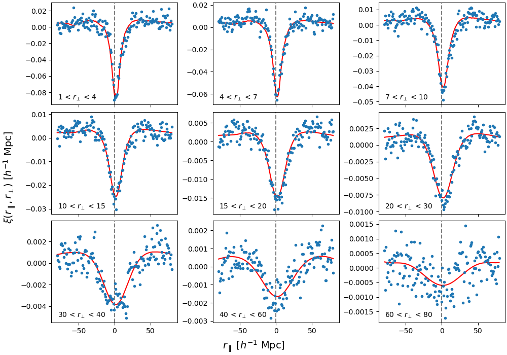
Figure 5: Measured Lyman-$\alpha$ forest and quasar cross-correlation (blue points) and resulting best-fit model for the baseline fit (red line). Both the correlation and the model are averaged in slices of $r_{\perp}$ and the $r_{\perp}$ slices (in  $h^{-1}$ Mpc) are shown in the lower left of each subplot. The dashed grey line represents $r_{\parallel}$ = 0. Seen in all $r_{\perp}$ slices is a shift of the correlation and model in the positive $r_{\parallel}$ direction, which is consistent with our results for $\Delta r_{\parallel}$.

The measured Lyman-$\alpha$ forest and quasar cross-correlation and the result for the baseline fit are presented in figure 5. We show the average of the correlation and model in each $r_{\perp}$ slice listed. The correlations have a lower amplitude for larger $r_{\perp}$ slices and therefore appear noisier. The model for the baseline fit is calculated jointly using the auto- and cross-correlations and has 13 free parameters. The values for the fixed parameters used in this model are presented in table 5 in Appendix A.

Parameter	Baseline	BAL	ZBAL
No. quasars	106,861	128,026	127,989
$b_{\text{Ly}\alpha}$	$-0.106\pm-0.023$	$-0.053\pm 0.011$	$-0.048\pm 0.009$
$\beta_{\text{Ly}\alpha}$	$1.8\pm 0.4$	$3.7\pm 0.7$	$4.0\pm 0.7$
$10^{3}b_{\eta,\text{SiII(1190)}}$	$-2.8\pm 0.9$	$-2.6\pm 0.8$	$-2.1\pm 1.0$
$10^{3}b_{\eta,\text{SiII(1193)}}$	$-0.3\pm 1.0$	$-0.0\pm 1.3$	$-0.0\pm 1.0$
$10^{3}b_{\eta,\text{SiIII(1207)}}$	$-2.6\pm 0.9$	$-1.9\pm 0.9$	$-1.2\pm 0.9$
$10^{3}b_{\eta,\text{SiII(1260)}}$	$-2.7\pm 1.2$	$-3.9\pm 1.6$	$-4.9\pm 1.7$
$b_{\text{HCD}}$	$-0.051\pm 0.008$	$-0.054\pm 0.010$	$-0.052\pm 0.011$
$b_{\text{q}}$	$3.1\pm 0.4$	$4.1\pm 0.4$	$4.4\pm 0.5$
$\Delta r_{\parallel}$ ($h^{-1}$Mpc)	$-1.94\pm 0.15$	$-1.84\pm 0.13$	$-1.90\pm 0.11$
$\sigma_{\text{v}}$ ($h^{-1}$Mpc)	$5.8\pm 0.5$	$7.3\pm 0.6$	$7.0\pm 0.6$
$\xi_{0}^{\text{TP}}$	$0.29\pm 0.05$	$0.08\pm 0.024$	$0.082\pm 0.023$
$10^{4}A_{\text{inst}}$	$2.28\pm 0.31$	$1.95\pm 0.27$	$1.90\pm 0.27$
$\chi^{2}$	1.036	1.042	1.037
$z_{\text{eff}}$	2.34	2.34	2.35

Table 2: Results of the fits for the baseline, BAL, and the ZBAL configurations. The number of quasars above $z=1.88$ in each catalog is given. In all fits the BAO parameters are fixed at 1.0. The rest of the parameters are allowed to float in each fit and are described in 5 in appendix A. Each fit has 11,644 data bins, 13 free parameters and we also list the effective redshift, $z_{\text{eff}}$. Since each fit is a joint fit of the auto- and cross-correlations, we list the $\chi^{2}$ value given for the joint fit.

We present the results of the baseline fit in the first column in table 2. The baseline fit has a joint $\chi^{2}$ value that corresponds to essentially zero probability. This is likely due to our model failing at small scale separations. We re-fit our model, increasing the minimum separation to $5\,h^{-1}\,\mathrm{Mpc}$ and $10\,h^{-1}\,\mathrm{Mpc}$ to check the results of the $\chi^{2}$ values. We found a very minimal improvement in $\chi^{2}$ values and a worsening of $\Delta r_{\parallel}$ values. We therefore decide to keep the minimum separation in our fit at $0\,h^{-1}\,\mathrm{Mpc}$ and leave for future studies any further tests of the model on $\chi^{2}$ values.

We find $\Delta r_{\parallel}$ $=-1.94\pm 0.15$ $h^{-1}$ Mpc and $\sigma_{\text{v}}=5.8\pm 0.5$ $h^{-1}$ Mpc. Comparing these results to table 1 of [14], we find that $\sigma_{\text{v}}$ is within 1.0$\sigma$ from the value reported in [14]. Our result for $\Delta r_{\parallel}$ is also consistent within 1.5$\sigma$ with [14], while our fit value for $\xi_{0}^{\text{TP}}$ is 2.0$\sigma$ with respect to the results reported in [14]. These differences are likely due to our smaller bin width, and the different ranges in $r_{\parallel}$ and $r_{\perp}$ used.

A negative value for $\Delta r_{\parallel}$ means the measured cross-correlation is shifted in the positive $r_{\parallel}$ direction, which is seen in all 9 $r_{\perp}$ slices in figure 5. Based on our definition of a positive separation, i.e, when the quasar is in front of the Lyman-$\alpha$ pixel, this indicates that the estimated quasar redshifts are less than the true quasar redshifts.

Our initial thought for this discrepancy is the disappearance of the MgII emission line from quasar spectra above redshift $z\approx 2.5$. The MgII line, a reliable indicator of systemic redshift [59, 39], is located beyond the observable range of the DESI spectrographs at these redshifts. We therefore rely on the high ionization broad lines, which often display significant velocity shifting [21], to obtain redshift estimates at $z>2.5$. This is also suggested by [29], who report a “kink" at $z\sim 2.5$ when comparing the redshift estimates from DESI to those from SDSS (their figure 16). However, this is unlikely the cause of the “kink" due to the observable range of the BOSS spectrographs being very similar to DESI [60], as eBOSS would lose access to the MgII line at similar redshifts to DESI.

The apparent underestimation of DESI redshifts persisted when updating the quasar templates in Redrock for processing the DESI year one quasar sample [27]. In section 6, we discuss the improvements in redshift performance for DESI year 1 data at $z>2$ when using an updated version of Redrock and quasar templates that properly model Lyman-$\alpha$ optical depth.

5.2 Dependence on Quasar Redshift

Parameter	z1	z2	z3	z4
No. quasars	41,688	27,958	17,407	19,808
Redshift range	$z\leq 2.2$	$2.2<z\leq 2.5$	$2.5<z\leq 2.8$	$z>2.8$
$b_{\text{Ly}\alpha}$	$-0.085\pm 0.010$	$-0.117\pm 0.009$	$-0.160\pm 0.011$	$-0.216\pm 0.015$
$\beta_{\text{Ly}\alpha}$	$1.77\pm 0.21$	$1.63\pm 0.17$	$1.48\pm 0.16$	$1.45\pm 0.15$
$10^{3}b_{\eta,\text{SiII(1190)}}$	$-3.6\pm 1.0$	$-2.6\pm 1.0$	$-3.2\pm 1.1$	$-3.4\pm 1.2$
$10^{3}b_{\eta,\text{SiII(1193)}}$	$-0.9\pm 0.9$	$-1.3\pm 1.0$	$-1.4\pm 1.1$	$-1.5\pm 1.2$
$10^{3}b_{\eta,\text{SiIII(1207)}}$	$-3.9\pm 0.9$	$-2.6\pm 0.9$	$-3.8\pm 1.0$	$-4.2\pm 1.2$
$10^{3}b_{\eta,\text{SiII(1260)}}$	$-2.8\pm 1.1$	$-2.6\pm 1.1$	$-2.9\pm 1.2$	$-3.1\pm 1.3$
$b_{\text{HCD}}$	$-0.037\pm 0.007$	$-0.049\pm 0.008$	$-0.053\pm 0.011$	$-0.067\pm 0.015$
$b_{\text{q}}$	$2.73\pm 0.29$	$2.88\pm 0.14$	$3.20\pm 0.23$	$4.1\pm 0.5$
$\Delta r_{\parallel}$ ($h^{-1}$Mpc)	$-1.07\pm 0.17$	$-1.99\pm 0.13$	$-3.5\pm 0.4$	$-3.4\pm 1.0$
$\sigma_{\text{v}}$ ($h^{-1}$Mpc)	$5.4\pm 0.7$	$5.5\pm 0.6$	$6.3\pm 1.0$	$8.1\pm 1.8$
$\xi_{0}^{\text{TP}}$	$0.13\pm 0.04$	$0.18\pm 0.04$	$0.51\pm 0.13$	$0.8\pm 0.4$
$A_{\text{inst}}$	$2.29\pm 0.29$	$2.38\pm 0.27$	$2.42\pm 0.27$	$2.42\pm 0.27$
$\chi^{2}_{\text{ JOINT}}$	1.033	1.030	1.030	1.053
$z_{\text{eff}}$	2.09	2.33	2.62	2.99

Table 3: Results of the fits for the four redshift evolution bins. The number of quasars in each bin is given, along with the redshift range of each bin. In all fits the BAO parameters are fixed at 1.0. The rest of the parameters are allowed to float in each fit and are described in table 5 in appendix A. Each fit has 11,644 data bins, 13 free parameters and we also list the effective redshift, $z_{\text{eff}}$. Since each fit is a joint fit of the auto- and cross-correlations, we list the $\chi^{2}$ value given for the joint fit.

We test and study here the evolution and dependence of the parameters $\Delta r_{\parallel}$ and $\sigma_{\text{v}}$ on quasar redshift to investigate more in depth the cause of the measured biases. We split the tracer quasar sample described in section 2 into four redshift bins: z1: $z\leq 2.2$, z2: $2.2<z\leq 2.5$, z3: $2.5<z\leq 2.8$, and z4: $z>2.8$. As a reminder, quasars with redshift $z<1.88$ will not contribute to the correlation as the separation will be larger than our maximum separation of $80\,h^{-1}\,\mathrm{Mpc}$. We use the same sample of Lyman-$\alpha$ forests as the baseline, but we create new quasar catalogs with approximately 41,000 objects in the first catalog, 28,000 objects in the second, 17,000 objects in the third, and 19,000 objects in the fourth. We then re-calculate the cross-correlation and fit for each redshift bin following the methods in section 3. Since the auto-correlation only depends on the Lyman-$\alpha$ forest sample, we do not need to re-compute it and can use the auto-correlation from [14] for each redshift bin when computing the joint fit.

The fit results for each redshift bin are given in table 3. Each fit has the same configuration as the baseline fit presented in the first column of table 2. We plot these results vs the average redshift in each bin in figure 6, highlighting the baseline value in the shaded region. We find a strong evolution with redshift for $\Delta r_{\parallel}$ with the value becoming more negative as the average redshift of the bin increases for the first three bins. However, the fourth redshift bin does not clearly follow this trend. Though this bin does not have the least amount of quasars, the quasars in this bin are at a higher redshift and are generally fainter and have lower signal to noise. The fit for this redshift bin is also the worst of the four with a $\chi^{2}=1.053$, which corresponds to near-zero probability given the 11,631 degrees of freedom in the fit. Despite this, the overall trend indicates that the quasar redshifts are being underestimated by a larger amount as the quasar redshift increases, which is consistent with the quasar templates not accounting for the Lyman-$\alpha$ forest optical depth. If the loss of the MgII emission line in the quasar spectra was the dominant contribution to the redshift errors, we would expect a sudden jump in $\Delta r_{\parallel}$ and $\sigma_{\text{v}}$ as a function of $z$ around $z=2.5$. Such a feature is not observed, so the loss of MgII is unlikely to be the culprit.

The measured evolution of $\sigma_{\texttt{v}}$ as a function of $z$ is much less striking than that of $\Delta r_{\parallel}$. Still, there is an indication for a mild increase of $\sigma_{\texttt{v}}$ for higher redshift quasars, consistent with less precision in the measured redshift.

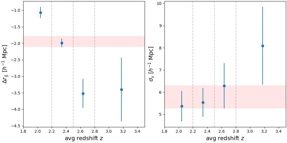
Figure 6: Evolution of $\Delta r_{\parallel}$ and $\sigma_{\text{v}}$ with redshift for four different redshift bins (blue points). The bin edges at z = 2.2, 2.5, and 2.8 are marked by the dashed grey lines. The red shaded region denotes the baseline value for each parameter: $\Delta r_{\parallel}$ = $-1.94\pm 0.15$ $h^{-1}$ Mpc and $\sigma_{\text{v}}=5.8\pm 0.5$ $h^{-1}$ Mpc.

5.3 Impact of BALs and Updating BAL Quasar Redshifts

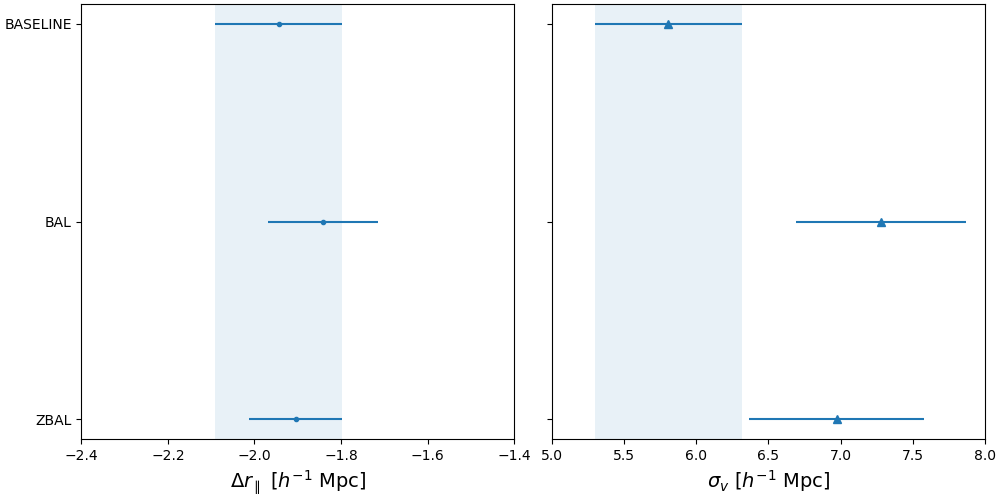
Figure 7: Results on $\Delta r_{\parallel}$ (left, blue points) and $\sigma_{\text{v}}$ (right, blue triangles) for the four different configurations presented in this work: baseline, BAL, and ZBAL. The shaded area represents the value of the parameters from the baseline fit.

BAL systems can impact the shape of quasar emission lines and introduce shifts in the estimated quasar redshift, up to several hundred km s^-1 [19]. BAL quasars often have larger redshift errors compared to quasars with no BAL features because the BAL features impact the blue side of emission lines [18]. This is true in DESI, where Redrock tends to overestimate redshifts for BAL quasars [18]. The current pipeline used for most Lyman-$\alpha$ studies, Picca, has the option to mask out BAL regions during the continuum fitting process, but does not update the quasar redshift when these masks are applied so any systematic errors on the quasar redshift will still be present. [19] shows that when BAL regions of a quasar spectrum are masked and new redshifts are obtained, those new redshifts shift by 240 km s^-1 on average. We explore in this section the effect of including the BAL quasars in the tracer catalog as well as using the updated BAL redshifts from [19] once the BAL regions of the quasar spectra are masked.

We first test if including BAL quasars in the tracer quasar catalog will have an effect on $\Delta r_{\parallel}$ or $\sigma_{\text{v}}$. For this test we use the same Lyman-$\alpha$ forest sample as [35] which is the same as our baseline. The tracer quasar catalog is the same as described in section 2.1 except the BALs are not removed. It consists of 128,026 quasars with redshift $z>1.88$. We use the auto-correlation from [14] and follow the same method described in section 3 to measure and fit the cross-correlation. We find $\Delta r_{\parallel}$ = $-1.84\pm 0.13$  $h^{-1}$ Mpc and $\sigma_{\text{v}}=7.3\pm 0.6$  $h^{-1}$ Mpc. These results, along with those from the baseline configuration, are shown in figure 7 and presented in table 2 in the BAL column. The shift of $\Delta r_{\parallel}$ in the positive direction would seem to indicate that including BAL quasars in the tracer catalog reduces the quasar redshift errors. However, this is actually due to BAL quasars typically having overestimated redshifts, as the BAL features tend to impact the blue side of the emission lines [18]. Any overestimation of quasar redshifts would shift $\Delta r_{\parallel}$ in the positive direction. This is the opposite of what we observe when the BAL quasars are excluded, where the shift in $\Delta r_{\parallel}$ is negative due to the underestimation of redshifts. It is likely that the inclusion of the BAL quasars partially compensates for the negative shift.

To test if updating the BAL quasar redshifts after the BAL regions are masked improves the $\Delta r_{\parallel}$ parameter, we use the quasar catalog from [19]. This is the same catalog as described above, but with updated redshifts for the BAL quasars, of which 28,185 BAL quasars have an updated redshift. Because the redshifts are updated, we can no longer use the Lyman-$\alpha$ forest sample described in [35]. We follow the method in [35] and in section 3 for the continuum fitting process and our final Lyman-$\alpha$ sample consists of 88,432 forests. We use the tracer catalog with updated redshifts and follow the method described in section 3 to measure and fit the correlations. We can no longer use the auto-correlation from [14], so we measure those following the method in [14]. The results are shown in figure 7 and in table 2 in the ZBAL column. We find $\Delta r_{\parallel}$ = $-1.90\pm 0.11$  $h^{-1}$ Mpc and $\sigma_{\text{v}}=7.0\pm 0.6$  $h^{-1}$ Mpc. The value of $\Delta r_{\parallel}$ has shifted in the negative direction and is now equal ($0.35\sigma$) to the baseline value. This negative shift is consistent with what is found in [19], which found that the redshifts of BAL quasars after masking were shifted to the blue.

This shows that BAL quasars can affect the correlations when they are included in the tracer catalog and their redshifts are not updated after the BAL regions are masked. When the redshifts are updated the inclusion of BAL quasars in the tracer catalog has no effect.

6 Addressing the Redshift Dependency

The redshift dependency in $\Delta r_{\parallel}$ is also reported in the year one quasar sample by [27], who suggest the bias could be mitigated through proper modeling of the mean transmission of Lyman-$\alpha$ in the spectral templates used for redshift estimation. We define the mean transmitted flux fraction, $\overline{F}$, as

$$\overline{F}(z)=e^{-\tau_{\text{eff},\alpha}(z)},$$ (6.1)

where

$$\tau_{\text{eff},\alpha}=\tau_{0}(1+z)^{\gamma}$$ (6.2)

is the effective optical depth of the Lyman-$\alpha$ transition, $\tau_{0}=(5.54\pm 0.64)\times 10^{-3}$ and $\gamma=3.182\pm 0.074$ [61]. $\overline{F}$ depends on $\tau_{\text{eff},\alpha}$ at $z=\frac{\lambda_{\text{obs}}-\lambda_{\text{Ly}\alpha}}{\lambda_{\text{Ly}\alpha}}$ according to eq. 6.1. $\tau_{\text{eff},\alpha}$ evolves with redshift, as parameterized by eq. 6.2 [e.g., 62, 63, 61], implying greater overall flux suppression in the Lyman-$\alpha$ forest region of quasar spectra at higher redshifts. The BOSS quasar templates used for EDR and the DESI year 1 quasar templates were derived from samples of quasar spectra that were not corrected for the optical depth of Lyman-$\alpha$ photons. On the other hand, a real-time correction for this flux suppression was being applied in Redrock during redshift fitting, leading to an over-suppression of template flux relative to what was expected at $\lambda_{\text{RF}}<1215.67$Å. This resulted in a bias that increases with the amount of suppression (i.e. redshift) at $z>2$.

We update the DESI year one quasar templates with the Lyman-$\alpha$ effective optical depth model from [61] and test whether the observed redshift bias is mitigated. The year one quasar templates consist of two eigenspectra sets which are trained to classify separate, yet overlapping redshift ranges: $0.05<z<1.6$ and $1.4<z<7.0$, dubbed LOZ and HIZ, respectively. As the Lyman-$\alpha$ forest is only observed in DESI quasar spectra with $z>1.95$, only the HIZ templates require modification. A new version of the HIZ templates are derived from the same sample as in [27], but the individual spectra are corrected for suppression from Lyman-$\alpha$ effective optical depth at $\lambda_{RF}<1215.67$Å. The Lyman-$\alpha$ optical depth model in Redrock was then updated accordingly. Our updated HIZ templates can be found on Github.

We use the updated HIZ templates with modified Redrock to refine the redshifts of the DESI year 1 quasar sample at $z>1.6$. This redshift is defined by the upper limit of the redshift coverage for the LOZ templates, though we note substantial impact is only expected at $z>1.95$. We impose a prior of $\Delta v=\pm 3000$ km s^-1 from the original redshift estimate, as the HIZ redshifts have been shown to be approximately correct within a few tens to hundreds of km s^-1, on average. Approximately 850,000 objects had a change in redshift when using the updated HIZ templates, and we show the distribution of those changes in figure 8.

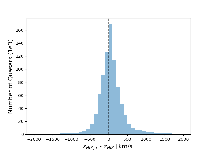
Figure 8: Distribution of the difference in redshift (in km s^-1) for the quasars in the year 1 catalog between the redshifts measured with the updated HIZ templates ($z_{\texttt{HIZ},\tau}$) versus the redshifts measured from the templates without the Lyman-$\alpha$ optical depth correction ($z_{\texttt{HIZ}}$).

To test that the redshift bias shown in $\Delta r_{\parallel}$ is mitigated we perform our analysis again using the updated quasar templates. We use the year 1 Lyman-$\alpha$ forest sample and tracer quasar catalog from [45]. To be consistent with our baseline analysis we remove any BAL quasars from the tracer catalog. There are 510,000 quasars in the tracer catalog with redshift $z>1.88$. We also split the tracer quasar sample to test for any evolution with redshift with the same cuts as in section 5.2: $z=2.2$, 2.5, and 2.8. We measure and fit the correlations using the same method described in section 3, and we show the results in table 4 and figure 9.

Parameter baseline z1 z2 z3 z4 No. quasars 510,501 201,290 138,364 82,710 88,137 Redshift range - $z\leq 2.2$ $2.2<z\leq 2.5$ $2.5<z\leq 2.8$ $z>2.8$ $b_{\text{Ly}\alpha}$ $-0.0543\pm 0.0035$ $-0.049\pm 0.005$ $-0.055\pm 0.005$ $-0.060\pm 0.006$ $-0.162\pm 0.020$ $\beta_{\text{Ly}\alpha}$ $3.78\pm 0.26$ $3.3\pm 0.4$ $3.8\pm 0.4$ $4.5\pm 0.5$ $2.01\pm 0.28$ $10^{3}b_{\eta,\text{SiII(1190)}}$ $-2.5\pm 0.4$ $-2.6\pm 0.4$ $-2.8\pm 0.4$ $-3.9\pm 0.5$ $-3.4\pm 0.5$ $10^{3}b_{\eta,\text{SiII(1193)}}$ $-1.34\pm 0.35$ $-1.3\pm 0.4$ $-2.2\pm 0.4$ $-2.0\pm 0.5$ $-2.2\pm 0.5$ $10^{3}b_{\eta,\text{SiIII(1207)}}$ $-4.50\pm 0.31$ $-5.0\pm 0.4$ $-5.0\pm 0.4$ $-6.0\pm 0.5$ $-5.4\pm 0.5$ $10^{3}b_{\eta,\text{SiII(1260)}}$ $-3.1\pm 0.6$ $-2.9\pm 0.5$ $-3.2\pm 0.6$ $-3.8\pm 0.7$ $-3.2\pm 0.6$ $b_{\text{HCD}}$ $-0.0574\pm 0.0034$ $-0.0491\pm 0.0029$ $-0.061\pm 0.004$ $-0.082\pm 0.005$ $-0.089\pm 0.006$ $b_{\text{q}}$ $3.97\pm 0.10$ $3.35\pm 0.13$ $3.99\pm 0.13$ $4.73\pm 0.17$ $4.35\pm 0.23$ $\Delta r_{\parallel}$ ($h^{-1}$Mpc) $-0.08\pm 0.04$ $-0.01\pm 0.06$ $-0.16\pm 0.07$ $-0.09\pm 0.08$ $-0.11\pm 0.13$ $\sigma_{\text{v}}$ ($h^{-1}$Mpc) $5.21\pm 0.17$ $4.79\pm 0.25$ $5.35\pm 0.25$ $5.45\pm 0.35$ $3.46\pm 0.35$ $\xi_{0}^{\text{TP}}$ $0.074\pm 0.008$ $0.066\pm 0.013$ $0.061\pm 0.014$ $0.114\pm 0.023$ $0.52\pm 0.09$ $10^{4}A_{\text{inst}}$ $1.33\pm 0.09$ $1.4\pm 0.1$ $1.36\pm 0.10$ $1.35\pm 0.10$ $1.51\pm 0.10$ $\chi^{2}_{\text{ JOINT}}$ 1.027 1.025 1.022 0.999 0.995 $z_{\text{eff}}$ 2.32 2.09 2.33 2.61 2.98

Table 4: Results of the fits using the updated quasar templates for the new baseline and four redshift bins. The number of quasars in each bin is given, along with the redshift range of each bin where applicable. The free parameters are the same as described in section 5. In all fits the BAO parameters are fixed at 1.0. Each fit has 11,644 data bins, 13 free parameters and we also list the effective redshift, $z_{\text{eff}}$. Since each fit is a joint fit of the auto- and cross-correlations, we list the $\chi^{2}$ value given for the joint fit.

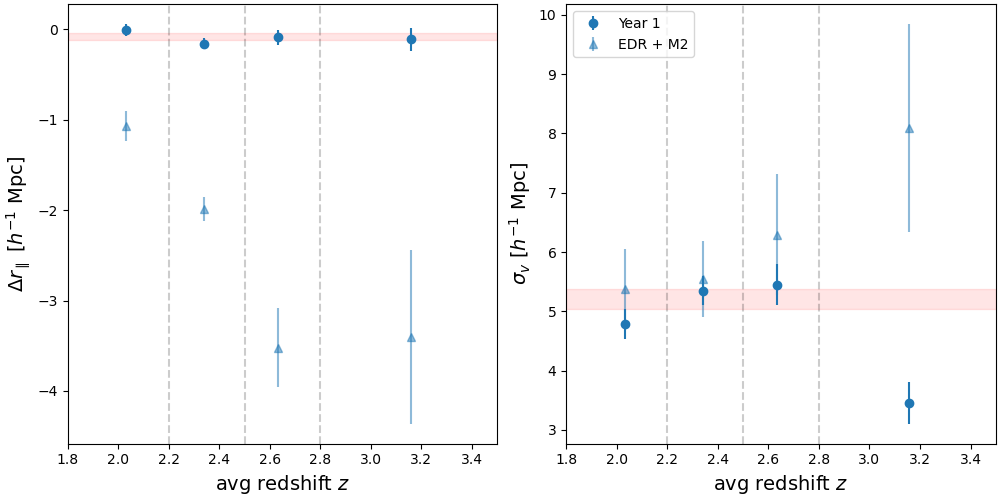
Figure 9: Evolution of $\Delta r_{\parallel}$ and $\sigma_{\text{v}}$ with redshift using the updated quasar templates for the four different redshift bins (blue points). The results with the old templates are shown in light blue triangles for comparison. The bin edges at z = 2.2, 2.5, and 2.8 are marked by the dashed grey lines. The red shaded region denotes the baseline value for each parameter: $\Delta r_{\parallel}$ = $-0.08\pm 0.04$ $h^{-1}$ Mpc and $\sigma_{\text{v}}=5.21\pm 0.17$ $h^{-1}$ Mpc.

We find $\Delta r_{\parallel}$ = $-0.08\pm 0.04$ $h^{-1}$ Mpc and $\sigma_{\text{v}}=5.21\pm 0.17$ $h^{-1}$ Mpc, which are shown as the red shaded region in figure 9. When testing for any evolution on $\Delta r_{\parallel}$ with redshift we find that the bias on $\Delta r_{\parallel}$ has been resolved. For the four redshift bins we find $\Delta r_{\parallel}$ [$h^{-1}$Mpc] = $-0.01\pm 0.06$, $-0.16\pm 0.07$, $-0.09\pm 0.08$, and $-0.11\pm 0.13$, respectively. The results for $\sigma_{\text{v}}$ also suggest a better precision on the measured redshifts. We find $\sigma_{\text{v}}$ [$h^{-1}$Mpc] = $4.79\pm 0.25$, $5.35\pm 0.25$, $5.45\pm 0.35$, and $3.46\pm 0.35$ for the four redshift bins, respectively.

Our updated HIZ templates and Redrock code have corrected the bias that was found using previous versions of the quasar templates and Redrock. The updated templates and Redrock will provide the redshifts for the DESI year one Lyman-$\alpha$ cosmology studies [45]. The redshifts will be publicly released with the year one quasar sample.

7 Summary

We present here the study of the impact of quasar redshift errors on the 3D Lyman-$\alpha$ forest-quasar cross-correlation. Using EDR+M2 data, the Lyman-$\alpha$ forest sample from [35], and the auto-correlation from [14], we compute the cross-correlation using a 1 $h^{-1}$ Mpc bin width up to 80 $h^{-1}$ Mpc in the $r_{\parallel}$ and $r_{\perp}$ directions. We validate our choice to use a 1 $h^{-1}$ Mpc bin width with mock data. Our model has 13 free parameters, of which $\Delta r_{\parallel}$ and $\sigma_{\text{v}}$ are used to quantify any systematic quasar redshift errors.

In our baseline fit we find $\Delta r_{\parallel}$ = $-1.94\pm 0.15$ $h^{-1}$ Mpc ($-205\pm 15~{}\text{km~{}s}^{-1}$) and $\sigma_{\text{v}}=5.8\pm 0.5$ $h^{-1}$ Mpc ($610\pm 50~{}\text{km~{}s}^{-1}$), which indicates that the EDR+M2 quasar redshifts are underestimated. It was reported in [27] that there is a redshift-dependent bias in the eBOSS quasar templates that likely stems from the improper correction of the Lyman-$\alpha$ forest optical depth. This introduces suppression in the Lyman-$\alpha$ forest that increases with redshift. We confirm that this bias is present in the EDR+M2 sample by measuring and fitting the cross-correlation when the tracer quasar catalog is cut into four redshift bins with boundaries at $z=$ 2.2, 2.5, and 2.8. We find $\Delta r_{\parallel}$ [$h^{-1}$ Mpc] = $-1.07\pm 0.17$, $-1.99\pm 0.13$, $-3.5\pm 0.4$, and $-3.4\pm 1.0$ for the four bins, respectively. This shows a redshift-dependent bias that increases with redshift.

New HIZ quasar templates were derived that corrected for the suppression from the Lyman-$\alpha$ effective optical depth. A modified version of Redrock was run with these new templates to update the DESI Year 1 quasar sample at $z>1.6$. We then repeat our analysis with the new Year 1 quasar redshifts to confirm that the bias in $\Delta r_{\parallel}$ is resolved. We find $\Delta r_{\parallel}$ = $-0.08\pm 0.04$  $h^{-1}$ Mpc ($-9.0\pm 4.0~{}\text{km~{}s}^{-1}$) and $\sigma_{\text{v}}=5.21\pm 0.17$ $h^{-1}$ Mpc ($-548\pm 17~{}\text{km~{}s}^{-1}$) when repeating the analysis on the entire year 1 quasar sample. We again split the catalog into four redshift bins with boundaries at $z=$ 2.2, 2.5, and 2.8 and we find $\Delta r_{\parallel}$ [$h^{-1}$ Mpc] = $-0.01\pm 0.06$, $-0.16\pm 0.07$, $-0.09\pm 0.08$, and $-0.11\pm 0.13$ for the four redshift bins, respectively.

We have shown that our updated HIZ quasar templates have mitigated the redshift bias on $\Delta r_{\parallel}$. These templates will be used to provide redshifts for the DESI year 1 quasar sample and those redshifts will be used for the Year 1 analyses.

Appendix A Fit Parameters

Parameter Value Description $\alpha_{\parallel},\alpha_{\perp}$ 1.0 BAO peak position parameters $A_{\text{peak}}$ 1.0 BAO amplitude (eq. 3.16) $b_{\text{q}}$ floating Quasar bias parameter (eq. 3.12) $\beta_{\text{q}}$ 0.323 Quasar RSD parameter (derived) (eq. 3.13) $\alpha_{\text{q}}$ 1.44 Redshift evolution parameter for $b_{\text{q}}$ (eq. 3.12) $b_{\text{Lya}}$ floating Lya absorber bias parameter (eq. 3.14) $\beta_{\text{Lya}}$ floating Lya absorber RSD parameter (3.15) $\alpha_{\text{Lya}}$ 2.9 Redshift evolution parameter for $b_{\text{Lya}}$ (eq. 3.12) $b_{\text{HCD}}$ floating bias parameter from unidentified HCD systems (eq. 3.15) $\beta_{\text{HCD}}$ floating RSD parameter from unidentified HCD systems (eq. 3.15) $L_{\text{HCD}}$ $10\,h^{-1}\,\mathrm{Mpc}$ Length scale from unidentified HCD systems (eq. 3.15) $b_{\text{m}}$ floating bias parameters for the metal species listed in table 1 $\beta_{\text{m}}$ 0.5 RSD parameters for the metal species listed in table 1 $\alpha_{\text{m}}$ 1.0 Redshift evolution parameter for metal biases $b_{\text{m}}$ $\sigma_{v}$ floating quasar non-linear velocity and precision (eq. 3.18) $\Delta r_{\parallel}$ floating the systematic offset in quasar redshift (eq. 3.23) $f$ 0.9703 linear growth rate of structure (eq. 3.17) $\Sigma$ = ($\Sigma_{\parallel}$, $\Sigma_{\perp}$) (6.37, 3.26) $h^{-1}$ Mpc Non-linear broadening of the BAO peak (eq. 3.16) R = ($R_{\parallel}$, $R_{\perp}$) (1, 1) $h^{-1}$ Mpc Smoothing parameters for the binning of the correlation (eq. 3.19) $\xi^{\text{TP}}_{0}$ floating Transverse proximity effect (eq. 3.22) $a_{\text{UV}},t_{\text{UV}}$ 0 Quasar radiation and anisotropy lifetime (eq. 3.22) $\lambda_{\text{UV}}$ $300\,h^{-1}\,\mathrm{Mpc}$ mean free path of UV photons (eq. 3.22) $A_{\text{inst}}$ floating Instrumental systematics parameter (equation 4.11 in [14])

Table 5: Parameters of the joint fit of the Lyman-$\alpha$ forest auto- and cross-correlations. The second column gives the value for each fixed parameter or if it is floating in the fit. The third column provides a brief description of each parameter and also a reference to the relevant equation. All biases $b$ refer to the bias calculated at the effective redshift ($z_{\text{eff}}=2.34$ for the baseline fit).

References

- [1] DESI Collaboration, A. Aghamousa, J. Aguilar, S. Ahlen, S. Alam, L. E. Allen et al., The DESI Experiment Part I: Science,Targeting, and Survey Design, arXiv e-prints (2016) arXiv:1611.00036 [1611.00036].
- [2] DESI Collaboration, A. Aghamousa, J. Aguilar, S. Ahlen, S. Alam, L. E. Allen et al., The DESI Experiment Part II: Instrument Design, arXiv e-prints (2016) arXiv:1611.00037 [1611.00037].
- [3] DESI Collaboration, B. Abareshi, J. Aguilar, S. Ahlen, S. Alam, D. M. Alexander et al., Overview of the Instrumentation for the Dark Energy Spectroscopic Instrument, AJ 164 (2022) 207 [2205.10939].
- [4] DESI Collaboration, A. G. Adame, J. Aguilar, S. Ahlen, S. Alam, G. Aldering et al., Validation of the Scientific Program for the Dark Energy Spectroscopic Instrument, AJ 167 (2024) 62 [2306.06307].
- [5] DESI Collaboration, A. G. Adame, J. Aguilar, S. Ahlen, S. Alam, G. Aldering et al., The Early Data Release of the Dark Energy Spectroscopic Instrument, arXiv e-prints (2023) arXiv:2306.06308 [2306.06308].
- [6] J. Hou, A. G. Sánchez, A. J. Ross, A. Smith, R. Neveux, J. Bautista et al., The completed SDSS-IV extended Baryon Oscillation Spectroscopic Survey: BAO and RSD measurements from anisotropic clustering analysis of the quasar sample in configuration space between redshift 0.8 and 2.2, Mon. Not. Roy. Astron. Soc. 500 (2021) 1201 [2007.08998].
- [7] R. Neveux, E. Burtin, A. de Mattia, A. Smith, A. J. Ross, J. Hou et al., The completed SDSS-IV extended Baryon Oscillation Spectroscopic Survey: BAO and RSD measurements from the anisotropic power spectrum of the quasar sample between redshift 0.8 and 2.2, Mon. Not. Roy. Astron. Soc. 499 (2020) 210 [2007.08999].
- [8] H. du Mas des Bourboux, J. Rich, A. Font-Ribera, V. de Sainte Agathe, J. Farr, T. Etourneau et al., The Completed SDSS-IV Extended Baryon Oscillation Spectroscopic Survey: Baryon Acoustic Oscillations with Ly Forests, ApJ 901 (2020) 153 [2007.08995].
- [9] N. G. Busca, T. Delubac, J. Rich, S. Bailey, A. Font-Ribera, D. Kirkby et al., Baryon acoustic oscillations in the Ly forest of BOSS quasars, Astron. Astrophys. 552 (2013) A96 [1211.2616].
- [10] A. Slosar, V. Iršič, D. Kirkby, S. Bailey, N. G. Busca, T. Delubac et al., Measurement of baryon acoustic oscillations in the Lyman- forest fluctuations in BOSS data release 9, JCAP 2013 (2013) 026 [1301.3459].
- [11] T. Delubac, J. E. Bautista, N. G. Busca, J. Rich, D. Kirkby, S. Bailey et al., Baryon acoustic oscillations in the Ly forest of BOSS DR11 quasars, Astron. Astrophys. 574 (2015) A59 [1404.1801].
- [12] A. Cuceu, A. Font-Ribera, S. Nadathur, B. Joachimi and P. Martini, Constraints on the Cosmic Expansion Rate at Redshift 2.3 from the Lyman- Forest, Phys. Rev. Lett. 130 (2023) 191003 [2209.13942].
- [13] S. Alam, M. Aubert, S. Avila, C. Balland, J. E. Bautista, M. A. Bershady et al., Completed SDSS-IV extended Baryon Oscillation Spectroscopic Survey: Cosmological implications from two decades of spectroscopic surveys at the Apache Point Observatory, Phys. Rev. D 103 (2021) 083533 [2007.08991].
- [14] C. Gordon, A. Cuceu, J. Chaves-Montero, A. Font-Ribera, A. X. González-Morales, J. Aguilar et al., 3D correlations in the Lyman- forest from early DESI data, JCAP 2023 (2023) 045 [2308.10950].
- [15] C. Ravoux, M. L. Abdul Karim, E. Armengaud, M. Walther, N. G. Karaçaylı, P. Martini et al., The Dark Energy Spectroscopic Instrument: one-dimensional power spectrum from first Ly forest samples with Fast Fourier Transform, Mon. Not. Roy. Astron. Soc. 526 (2023) 5118 [2306.06311].
- [16] N. G. Karaçaylı, P. Martini, J. Guy, C. Ravoux, M. L. Abdul Karim, E. Armengaud et al., Optimal 1D Ly forest power spectrum estimation - III. DESI early data, Mon. Not. Roy. Astron. Soc. 528 (2024) 3941 [2306.06316].
- [17] N. G. Karaçaylı, P. Martini, D. H. Weinberg, V. Iršič, J. Aguilar, S. Ahlen et al., A framework to measure the properties of intergalactic metal systems with two-point flux statistics, Mon. Not. Roy. Astron. Soc. 522 (2023) 5980 [2302.06936].
- [18] L. Á. García, P. Martini, A. X. Gonzalez-Morales, A. Font-Ribera, H. K. Herrera-Alcantar, J. N. Aguilar et al., Analysis of the impact of broad absorption lines on quasar redshift measurements with synthetic observations, Mon. Not. Roy. Astron. Soc. 526 (2023) 4848 [2304.05855].
- [19] S. Filbert, P. Martini, K. Seebaluck, L. Ennesser, D. M. Alexander, A. Bault et al., Broad Absorption Line Quasars in the Dark Energy Spectroscopic Instrument Early Data Release, arXiv e-prints (2023) arXiv:2309.03434 [2309.03434].
- [20] C. M. Gaskell, A redshift difference between high and low ionization emission-line regions in QSO’s-evidence for radial motions., ApJ 263 (1982) 79.
- [21] Y. Shen, W. N. Brandt, G. T. Richards, K. D. Denney, J. E. Greene, C. J. Grier et al., The Sloan Digital Sky Survey Reverberation Mapping Project: Velocity Shifts of Quasar Emission Lines, ApJ 831 (2016) 7 [1602.03894].
- [22] G. T. Richards, D. E. Vanden Berk, T. A. Reichard, P. B. Hall, D. P. Schneider, M. SubbaRao et al., Broad Emission-Line Shifts in Quasars: An Orientation Measure for Radio-Quiet Quasars?, AJ 124 (2002) 1 [astro-ph/0204162].
- [23] J. Guy, S. Bailey, A. Kremin, S. Alam, D. M. Alexander, C. Allende Prieto et al., The Spectroscopic Data Processing Pipeline for the Dark Energy Spectroscopic Instrument, AJ 165 (2023) 144 [2209.14482].
- [24] S. Bailey et al., Redrock: Spectroscopic Classification and Redshift Fitting for the Dark Energy Spectroscopic Instrument, in prep .
- [25] A. S. Bolton, D. J. Schlegel, É. Aubourg, S. Bailey, V. Bhardwaj, J. R. Brownstein et al., Spectral Classification and Redshift Measurement for the SDSS-III Baryon Oscillation Spectroscopic Survey, AJ 144 (2012) 144 [1207.7326].
- [26] D. M. Alexander, T. M. Davis, E. Chaussidon, V. A. Fawcett, A. X. Gonzalez-Morales, T.-W. Lan et al., The DESI Survey Validation: Results from Visual Inspection of the Quasar Survey Spectra, AJ 165 (2023) 124 [2208.08517].
- [27] A. Brodzeller, K. Dawson, S. Bailey, J. Yu, A. J. Ross, A. Bault et al., Performance of the Quasar Spectral Templates for the Dark Energy Spectroscopic Instrument, AJ 166 (2023) 66 [2305.10426].
- [28] S. Youles, J. E. Bautista, A. Font-Ribera, D. Bacon, J. Rich, D. Brooks et al., The effect of quasar redshift errors on Lyman- forest correlation functions, Mon. Not. Roy. Astron. Soc. 516 (2022) 421 [2205.06648].
- [29] E. Chaussidon, C. Yèche, N. Palanque-Delabrouille, D. M. Alexander, J. Yang, S. Ahlen et al., Target Selection and Validation of DESI Quasars, ApJ 944 (2023) 107 [2208.08511].
- [30] N. Busca and C. Balland, QuasarNET: Human-level spectral classification and redshifting with Deep Neural Networks, arXiv e-prints (2018) arXiv:1808.09955 [1808.09955].
- [31] J. Farr, A. Font-Ribera and A. Pontzen, Optimal strategies for identifying quasars in DESI, JCAP 2020 (2020) 015 [2007.10348].
- [32] D. Green et al.in prep (2024) .
- [33] A. D. Myers, J. Moustakas, S. Bailey, B. A. Weaver, A. P. Cooper, J. E. Forero-Romero et al., The Target-selection Pipeline for the Dark Energy Spectroscopic Instrument, AJ 165 (2023) 50 [2208.08518].
- [34] Z. Guo and P. Martini, Classification of Broad Absorption Line Quasars with a Convolutional Neural Network, ApJ 879 (2019) 72 [1901.04506].
- [35] C. Ramírez-Pérez, I. Pérez-Ràfols, A. Font-Ribera, M. A. Karim, E. Armengaud, J. Bautista et al., The Lyman- forest catalog from the Dark Energy Spectroscopic Instrument Early Data Release, Mon. Not. Roy. Astron. Soc. (2023) [2306.06312].
- [36] J. Zou et al., in prep, .
- [37] Planck Collaboration, N. Aghanim, Y. Akrami, M. Ashdown, J. Aumont, C. Baccigalupi et al., Planck 2018 results. VI. Cosmological parameters, Astron. Astrophys. 641 (2020) A6 [1807.06209].
- [38] A. Font-Ribera, J. Miralda-Escudé, E. Arnau, B. Carithers, K.-G. Lee, P. Noterdaeme et al., The large-scale cross-correlation of Damped Lyman alpha systems with the Lyman alpha forest: first measurements from BOSS, JCAP 2012 (2012) 059 [1209.4596].
- [39] A. Font-Ribera, E. Arnau, J. Miralda-Escudé, E. Rollinde, J. Brinkmann, J. R. Brownstein et al., The large-scale quasar-Lyman forest cross-correlation from BOSS, JCAP 2013 (2013) 018 [1303.1937].
- [40] N. Kaiser, Clustering in real space and in redshift space, Mon. Not. Roy. Astron. Soc. 227 (1987) 1.
- [41] H. du Mas des Bourboux, K. S. Dawson, N. G. Busca, M. Blomqvist, V. de Sainte Agathe, C. Balland et al., The Extended Baryon Oscillation Spectroscopic Survey: Measuring the Cross-correlation between the Mg II Flux Transmission Field and Quasars and Galaxies at z = 0.59, ApJ 878 (2019) 47 [1901.01950].
- [42] P. McDonald, U. Seljak, S. Burles, D. J. Schlegel, D. H. Weinberg, R. Cen et al., The Ly Forest Power Spectrum from the Sloan Digital Sky Survey, ApJS 163 (2006) 80 [astro-ph/0405013].
- [43] A. Font-Ribera and J. Miralda-Escudé, The effect of high column density systems on the measurement of the Lyman- forest correlation function, JCAP 2012 (2012) 028 [1205.2018].
- [44] K. K. Rogers, S. Bird, H. V. Peiris, A. Pontzen, A. Font-Ribera and B. Leistedt, Correlations in the three-dimensional Lyman-alpha forest contaminated by high column density absorbers, Mon. Not. Roy. Astron. Soc. 476 (2018) 3716 [1711.06275].
- [45] DESI Collaboration, DESI 2024 IV: Baryon Acoustic Oscillations from the Lyman Alpha Forest, in preparation (2024) .
- [46] D. Kirkby, D. Margala, A. Slosar, S. Bailey, N. G. Busca, T. Delubac et al., Fitting methods for baryon acoustic oscillations in the Lyman- forest fluctuations in BOSS data release 9, JCAP 2013 (2013) 024 [1301.3456].
- [47] A. Lewis, A. Challinor and A. Lasenby, Efficient Computation of Cosmic Microwave Background Anisotropies in Closed Friedmann-Robertson-Walker Models, ApJ 538 (2000) 473 [astro-ph/9911177].
- [48] D. J. Eisenstein, H.-J. Seo and M. White, On the Robustness of the Acoustic Scale in the Low-Redshift Clustering of Matter, ApJ 664 (2007) 660 [astro-ph/0604361].
- [49] A. Arinyo-i-Prats, J. Miralda-Escudé, M. Viel and R. Cen, The non-linear power spectrum of the Lyman alpha forest, JCAP 2015 (2015) 017 [1506.04519].
- [50] H. du Mas des Bourboux, J.-M. Le Goff, M. Blomqvist, N. G. Busca, J. Guy, J. Rich et al., Baryon acoustic oscillations from the complete SDSS-III Ly-quasar cross-correlation function at z = 2.4, Astron. Astrophys. 608 (2017) A130 [1708.02225].
- [51] J. E. Bautista, N. G. Busca, J. Guy, J. Rich, M. Blomqvist, H. du Mas des Bourboux et al., Measurement of baryon acoustic oscillation correlations at z = 2.3 with SDSS DR12 Ly-Forests, Astron. Astrophys. 603 (2017) A12 [1702.00176].
- [52] M. Blomqvist, M. M. Pieri, H. du Mas des Bourboux, N. G. Busca, A. Slosar, J. E. Bautista et al., The triply-ionized carbon forest from eBOSS: cosmological correlations with quasars in SDSS-IV DR14, JCAP 2018 (2018) 029 [1801.01852].
- [53] G. C. Rudie, C. C. Steidel, A. E. Shapley and M. Pettini, The Column Density Distribution and Continuum Opacity of the Intergalactic and Circumgalactic Medium at Redshift langzrang = 2.4, ApJ 769 (2013) 146 [1304.6719].
- [54] F. Lepori, V. Iršič, E. Di Dio and M. Viel, The impact of relativistic effects on the 3D Quasar-Lyman- cross-correlation, JCAP 2020 (2020) 006 [1910.06305].
- [55] M. Blomqvist, H. du Mas des Bourboux, N. G. Busca, V. de Sainte Agathe, J. Rich, C. Balland et al., Baryon acoustic oscillations from the cross-correlation of Ly absorption and quasars in eBOSS DR14, Astron. Astrophys. 629 (2019) A86 [1904.03430].
- [56] H. K. Herrera-Alcantar, A. Muñoz-Gutiérrez, T. Tan, A. X. González-Morales, A. Font-Ribera, J. Guy et al., Synthetic spectra for Lyman- forest analysis in the Dark Energy Spectroscopic Instrument, arXiv e-prints (2023) arXiv:2401.00303 [2401.00303].
- [57] T. Etourneau, J.-M. Le Goff, J. Rich, T. Tan, A. Cuceu, S. Ahlen et al., Mock data sets for the Eboss and DESI Lyman- forest surveys, arXiv e-prints (2023) arXiv:2310.18996 [2310.18996].
- [58] W. J. Percival and M. White, Testing cosmological structure formation using redshift-space distortions, Mon. Not. Roy. Astron. Soc. 393 (2009) 297 [0808.0003].
- [59] P. C. Hewett and V. Wild, Improved redshifts for SDSS quasar spectra, Mon. Not. Roy. Astron. Soc. 405 (2010) 2302 [1003.3017].
- [60] S. A. Smee, J. E. Gunn, A. Uomoto, N. Roe, D. Schlegel, C. M. Rockosi et al., The Multi-object, Fiber-fed Spectrographs for the Sloan Digital Sky Survey and the Baryon Oscillation Spectroscopic Survey, AJ 146 (2013) 32 [1208.2233].
- [61] V. Kamble, K. Dawson, H. du Mas des Bourboux, J. Bautista and D. P. Scheinder, Measurements of Effective Optical Depth in the Ly Forest from the BOSS DR12 Quasar Sample, ApJ 892 (2020) 70 [1904.01110].
- [62] T. S. Kim, J. S. Bolton, M. Viel, M. G. Haehnelt and R. F. Carswell, An improved measurement of the flux distribution of the Ly forest in QSO absorption spectra: the effect of continuum fitting, metal contamination and noise properties, Mon. Not. Roy. Astron. Soc. 382 (2007) 1657 [0711.1862].
- [63] F. Calura, E. Tescari, V. D’Odorico, M. Viel, S. Cristiani, T. S. Kim et al., The Lyman forest flux probability distribution at z>3, Mon. Not. Roy. Astron. Soc. 422 (2012) 3019 [1201.5121].