Characterization of birefringence inhomogeneity of KAGRA sapphire mirrors from transmitted wavefront error measurements

Abstract

Future gravitational wave detectors are going to cool down their test masses to cryogenic temperatures to reduce thermal noise. Crystalline materials are considered most promising for making test masses and their coatings due to their excellent thermal and optical properties at low temperatures. However, birefringence due to local impurities and inhomogeneities in the crystal can degrade the performance of the detector. Birefringence measurement, or birefringence mapping over a two-dimensional area has become important. This paper describes a method of fast birefringence measurement for a large sample by simply combining a series of transmission wavefront error measurements using linearly polarized light with Fizeau interferometers. With this method, the birefringence inhomogeneity of two KAGRA’s input test masses with diameter of 22 cm is fully reconstructed. The birefringence information is then used to calculate the transverse beam shape of the light fields in orthogonal polarization directions when passing through the substrate. The calculated beam shapes show a good match with in-situ measurements using KAGRA interferometer. This technique is crucial for birefringence characterization of test masses in future detectors where even larger size are used.

I Introduction

Thermal noise is one of the main noise sources for future gravitational wave detectors [1, 2]. To reduce thermal noise, future detectors like LIGO Voyager [3] and Einstein Telescope [4, 5] are designed to operate at cryogenic temperatures. Cosmic Explorer [6] also considers cryogenic operation for an upgrade. KAGRA [7, 8, 9, 10] is the only one operating at cryogenic temperatures and pioneering this technique among current large scale ground-based detectors. All these detectors apply large size high-quality mirrors as their test masses forming optical resonators to sense the tiny length fluctuations introduced by gravitational waves. Fused silica is commonly used to make test masses at room temperature, but it is not compatible with low temperatures. Crystalline materials are considered most promising to make cryogenic test masses. Sapphire was selected as the material for KAGRA’s test masses [11] due to its excellent thermal and optical properties at low temperature [12, 13]. However, recent studies reveal that birefringence of crystalline substrates and coatings can degrade the performance of the detector [14, 15, 16, 17, 18, 19]. In this case, the birefringence fluctuates in magnitude and direction throughout the substrate of the mirror. Therefore, it is necessary to measure the position dependence of the birefringence over a large area to assess its impact on the optical performance.

There are many studies on two-dimensional birefringence measurements for transparent materials [14, 15, 20, 21, 22, 23, 24]. These measurements are either using a single-beam scanning technique, or expanding the beam to a large aperture and imaging with a sensor array. The scanning method is rather time-consuming for large size samples, e.g., mirrors with diameters usually more than 20 cm for ground-based gravitational wave detectors, if one wants to obtain good spatial resolution [25, 26]. The phase-shifting method in digital interferometry has been previously proposed for fast 2D birefringence measurements with a very high accuracy [27, 28, 29]. Fizeau interferometers are one of the most accurate methods to extract the phase information of an optical component (reflection phase or transmission phase) over a large area. Transmission Wavefront Error (TWE) is often used to measure the refractive index homogeneity of a substrate under test. In the presence of birefringence, however, a simple TWE measurement does not reveal the entire information about the substrate.

In this paper we describe a method of combining a series of TWE map measurements using linearly polarized light in an appropriate way to fully reconstruct the refractive index information including birefringence. With this method, the birefringence inhomogeneity of two KAGRA’s input test masses (ITM) is extracted. This birefringence information is then used to calculate the transverse beam shape of the light fields in orthogonal polarization directions when passing through the substrate. The calculated beam shapes show a good match with in-situ beam shape measurements. The method of extracting birefringence information from TWE measurements with Fizeau interferometers is introduced in Section II. Birefringence characterization of KAGRA’s current ITMs is described in Section III. Our conclusions are summarized in Section IV.

II Generating a birefringence map with a Fizeau interferometer

Figure 1 shows a schematic of a Fizeau interferometer. We analyze the interference pattern between the light reflected by the reference plane 1 ($E_{\mathrm{1}}$) and the light reflected by the reference plane 2 ($E_{\mathrm{2}}$) on the CCD. By comparing the results with and without the sample inserted into the cavity formed by the reference planes 1 and 2, we can obtain the information about the optical thickness of the sample. Since the optical thickness is the physical thickness times the index of refraction, by measuring the surface figure maps of S1 (surface with anti-reflecting coating) and S2 (surface with highly-reflective coating) precisely and subtracting out the variation of physical thickness of the sample, we can extract the fluctuation of the index of refraction in the substrate.

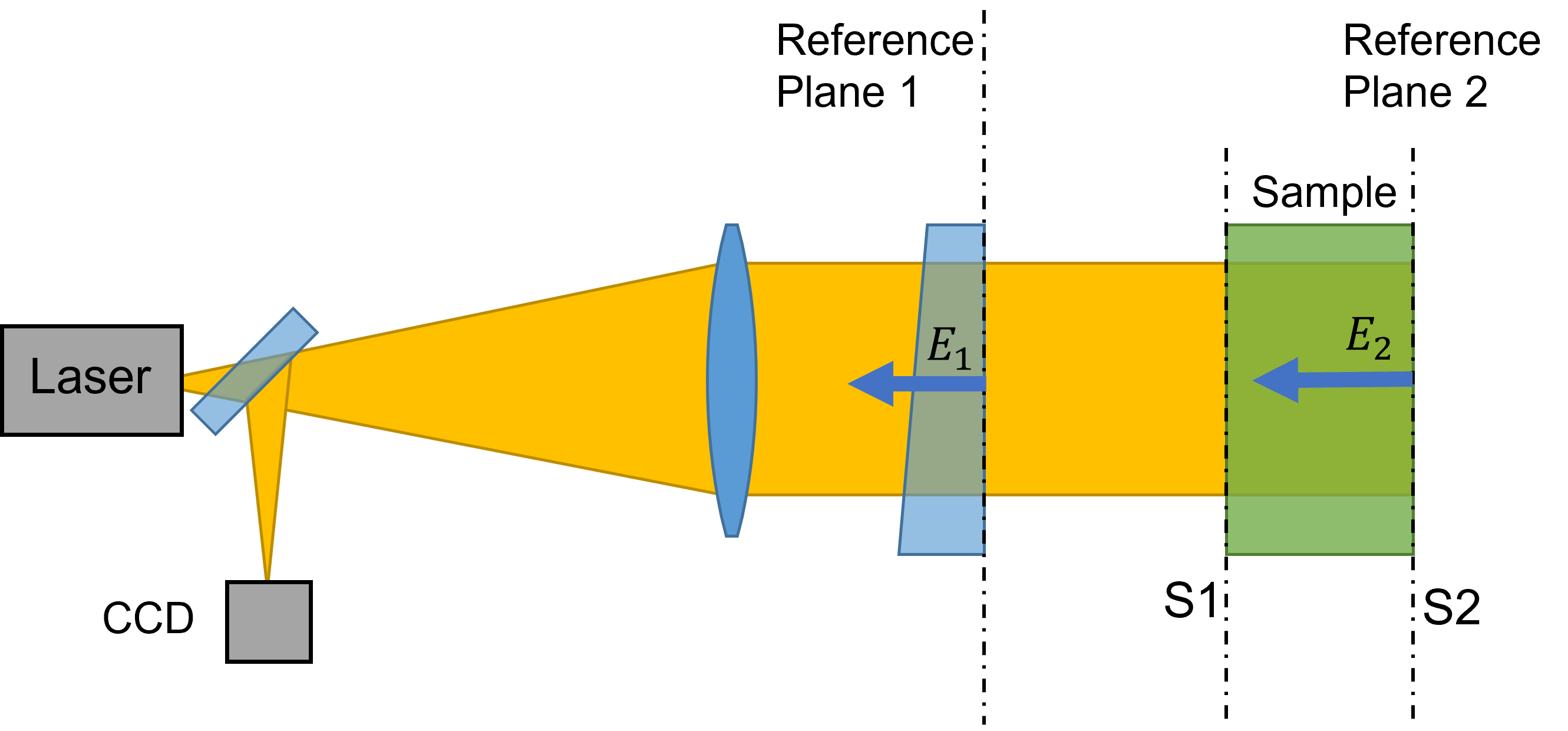
Figure 1: Schematic of TWE measurement with a Fizeau interferometer. S1 is the surface with anti-reflecting coating and S2 is the surface with highly-reflective coating. The interference between light fields $E_{\mathrm{1}}$ and $E_{\mathrm{2}}$ reflected by reference planes 1 and 2 respectively gives the TWE information of the sample.

In order to extract the birefringence information, measurements have to be performed using a linearly polarized light. To understand the behavior of such measurements, let us first consider what happens to a linearly polarized light going through a birefringent substrate.

II.1 Transmission of a linearly polarized light through a birefringent medium

Let us concentrate on an optical axis going through a single column of the substrate as shown in Figure 2. We define our preferred polarization axes called s and p in the vertical and horizontal directions with respect to the laboratory frame. The extra-ordinary and ordinary axes of the crystal in that particular column is assumed to be rotated by an angle $\theta$ with respect to our polarization axes. The input beam to the Fizeau interferometer is purely polarized in s ($E_{\mathrm{s}}$).

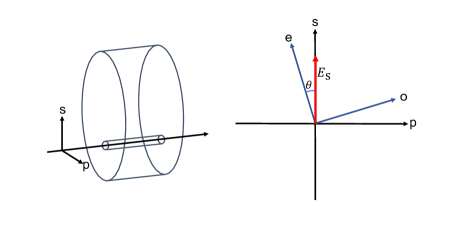
Figure 2: Transmission of a linearly polarized optical field through a column of a sample substrate.

We will use the Jones matrix formalism to analyze the conversion of the polarization state [30]. Here, the polarization state of light is represented by a vector,

$$\vec{V}=\begin{pmatrix}E_{\mathrm{s}}\\ E_{\mathrm{p}}\end{pmatrix},$$ (1)

where $E_{\mathrm{s}}$ and $E_{\mathrm{p}}$ are the complex amplitudes of s- and p-polarized electric fields.

After passing through the substrate twice (a round trip through the substrate), the polarization state is converted to

$$\vec{V}^{\prime}=M\cdot\vec{V},\quad\mathrm{with}\quad M=e^{i\alpha_{+}}\begin{pmatrix}e^{i\alpha_{-}}\cos^{2}\theta+e^{-i\alpha_{-}}\sin^{2}\theta&-i\sin\alpha_{-}\sin 2\theta\\ -i\sin\alpha_{-}\sin 2\theta&e^{-i\alpha_{-}}\cos^{2}\theta+e^{i\alpha_{-}}\sin^{2}\theta\end{pmatrix},$$ (2)

where $M$ is the round-trip Jones matrix of the substrate. We denote the indices of refraction for the extra-ordinary and ordinary axes as $n_{\mathrm{e}}$ and $n_{\mathrm{o}}$, respectively. Then we can compute the round trip phase changes of optical fields polarized in those axes:

$$\alpha_{\mathrm{e}}\equiv 2\pi\frac{2dn_{\mathrm{e}}}{\lambda},$$ (3)

$$\alpha_{\mathrm{o}}\equiv 2\pi\frac{2dn_{\mathrm{o}}}{\lambda},$$ (4)

where $d$ is the thickness of the substrate, $\lambda$ is the wavelength of the light.

Using $\alpha_{\mathrm{e}}$ and $\alpha_{\mathrm{o}}$, we define the common and differential phase changes,

$$\alpha_{+}\equiv\frac{\alpha_{\mathrm{e}}+\alpha_{\mathrm{o}}}{2},$$ (5)

$$\alpha_{-}\equiv\frac{\alpha_{\mathrm{e}}-\alpha_{\mathrm{o}}}{2}.$$ (6)

In most cases, the common phase is not important and we will ignore $\alpha_{+}$ in the following discussion. Note that the Jones matrix also works for a non-uniform medium (discussed in Appendix A).

For a purely s-polarized input field, $\vec{V}=(1,0)^{\mathrm{T}}$, the field returning from the substrate becomes,

$$\vec{V}^{\prime}=\begin{pmatrix}E_{\mathrm{s}}\\ E_{\mathrm{p}}\end{pmatrix}=\begin{pmatrix}e^{i\alpha_{-}}\cos^{2}\theta+e^{-i\alpha_{-}}\sin^{2}\theta\\ -i\sin\alpha_{-}\sin 2\theta\end{pmatrix}.$$ (7)

This $\vec{V}^{\prime}$ is the same as the field $E_{2}$ in Figure 1 at the CCD, except for the common phase term, which is ignored.

II.2 Interference with the reference field

The field $\vec{V}^{\prime}$ computed above is superposed with the reference field ($E_{1}$ in Figure 1). The reference field $\vec{V}_{\mathrm{r}}$ is purely polarized in s and has a certain phase offset $\phi$ from $\vec{V}^{\prime}$,

$$\vec{V}_{\mathrm{r}}=\begin{pmatrix}E_{\mathrm{r}}\\ 0\end{pmatrix}=\begin{pmatrix}e^{i\phi}\\ 0\end{pmatrix}.$$ (8)

The optical power detected by the CCD after the interference of $\vec{V}^{\prime}$ and $\vec{V}_{\mathrm{r}}$ is,

$$P=(\vec{V}_{\mathrm{r}}+\vec{V}^{\prime})\cdot(\vec{V}_{\mathrm{r}}+\vec{V}^{\prime})^{*}.$$ (9)

By plugging Equations 7 and 8 into Equation 9, we get,

$$P =|E_{\mathrm{s}}+E_{\mathrm{r}}|^{2}+|E_{\mathrm{p}}|^{2}$$

$$=|E_{\mathrm{s}}|^{2}+|E_{\mathrm{p}}|^{2}+|E_{\mathrm{r}}|^{2}+E_{\mathrm{s}}E_{\mathrm{r}}^{*}+E_{\mathrm{s}}^{*}E_{\mathrm{r}}.$$ (10)

From the conservation of energy, $|E_{\mathrm{s}}|^{2}+|E_{\mathrm{p}}|^{2}=1$. From Equation 8, $|E_{\mathrm{r}}|^{2}=1$. We will ignore those constant terms in the following discussion. Then what is interesting to us is,

$$\Delta P =E_{\mathrm{s}}E_{\mathrm{r}}^{*}+E_{\mathrm{s}}^{*}E_{\mathrm{r}}$$

$$=2\cos^{2}\theta\cos(\phi-\alpha_{-})+2\sin^{2}\theta\cos(\phi+\alpha_{-}).$$ (11)

If the s-polarization axis is aligned with the extra-ordinary axis ($\theta=0$), $\Delta P=2\cos(\phi-\alpha_{-})$. Usually, a Fizeau interferometer is equipped with a mechanism to change the position of the reference plane 1, for example, by mounting the reference flat on a piezo stage. Therefore, we can scan the relative phase $\phi$ by known amounts and fit the measured variation of $\Delta P$ to know the value of $\alpha_{-}$. In the general case of $\theta\neq 0$, the Fizeau measurement obtains the phase of the field $E_{\mathrm{s}}$, i.e. $\psi=\arg(E_{\mathrm{s}})$.

II.3 Extraction of $\alpha_{-}$ and $\theta$ from several TWE maps

When the orientation of the extra-ordinary axis is not known, which is almost always the case, we need to take several TWE maps with different orientation of the sample or the measurement beam polarization. Then combine them to extract $\theta$ and $\alpha_{-}$.

As explained in the previous section, a TWE measurement by a Fizeau interferometer yields a transmission phase $\psi$ at each point on the sample surface. Let us assume that we rotate the sample by an angle $\eta$, or equivalently the input polarization orientation by $-\eta$. This is equivalent to changing the orientation of the extra-ordinary axis from $\theta$ to $\theta+\eta$.

Let us denote the measured phase with an $\eta$ rotation of the sample as $\psi(\eta)$. From Equation 7,

$$\psi(\eta) =\arg\left[E_{\mathrm{s}}(\theta+\eta)\right]$$

$$=\arg\left[\cos^{2}(\theta+\eta)e^{i\alpha_{-}}+\sin^{2}(\theta+\eta)e^{-i\alpha_{-}}\right]$$

$$=\arctan\left[\cos(2\theta+2\eta)\tan\alpha_{-}\right].$$ (12)

We can see $\psi(\eta)$ as a function of $\eta$ with parameters $\theta$ and $\alpha_{-}$ determining its shape. Therefore, if we have several measurements of $\psi(\eta)$ with different values of $\eta$, we can use a non-linear fitting algorithm to fit the measured values with Equation 12 to obtain the best fit values of $\theta$ and $\alpha_{-}$.

If $\alpha_{-}$ can be assumed to be very small, which is the case for KAGRA mirrors, we can expand Equation 12 with $\alpha_{-}$, leaving only the $\mathcal{O}(\alpha_{-})$ terms, as

$$\psi(\eta) \sim\cos(2\theta+2\eta)\alpha_{-}$$

$$=\left(\cos(2\theta)\cos(2\eta)-\sin(2\theta)\sin(2\eta)\right)\alpha_{-}.$$ (13)

Assuming that we have four measurements of $\psi(\eta)$ with four different values of $\eta=\eta_{1},\eta_{2},\eta_{3},\eta_{4}$, we compute the following quantities,

$$\Delta\psi_{1} \equiv\psi(\eta_{1})-\psi(\eta_{2})=\alpha_{-}\left(A\cos 2\theta-B\sin 2\theta\right)$$ (14)

$$\Delta\psi_{2} \equiv\psi(\eta_{3})-\psi(\eta_{4})=\alpha_{-}\left(C\cos 2\theta-D\sin 2\theta\right),$$ (15)

where,

$$A =\cos 2\eta_{1}-\cos 2\eta_{2}$$ (16)

$$B =\sin 2\eta_{1}-\sin 2\eta_{2}$$ (17)

$$C =\cos 2\eta_{3}-\cos 2\eta_{4}$$ (18)

$$D =\sin 2\eta_{3}-\sin 2\eta_{4}.$$ (19)

We then take the ratio of $\Delta\psi_{1}$ and $\Delta\psi_{2}$,

$$r \equiv\frac{\Delta\psi_{1}}{\Delta\psi_{2}}=\frac{A\cos 2\theta-B\sin 2\theta}{C\cos 2\theta-D\sin 2\theta}=\frac{A-B\tan 2\theta}{C-D\tan 2\theta}.$$ (20)

Solving the above for $\theta$,

$$\theta=\frac{1}{2}\arctan\left(\frac{A-rC}{B-rD}\right).$$ (21)

Once the value of $\theta$ is obtained, we can use Equation 12 to compute the value of $\alpha_{-}$ as,

$$\alpha_{-}=\arctan\left[\frac{\tan\left\{\psi(\eta)\right\}}{\cos(2\theta+2\eta)}\right].$$ (22)

III Birefringence characterization of KAGRA sapphire ITMs

Sapphire is a uniaxial crystal with optical axis called c-axis. KAGRA’s sapphire test masses are fabricated so that the input surface is perpendicular to the c-axis. Light propagating in the test mass substrate will travel along the c-axis and there should be no birefringence in theory. However, local impurities and inhomogeneities in the crystal, and also mechanical and thermal stress changes (e.g., due to the suspension system supporting the mirror) can cause depolarization. These local defects will distort the polarization distribution of the light field in the transverse plane. From Equation 2 we can see the cross-coupling term $E_{\mathrm{p}}=-i\sin\alpha_{-}\sin 2\theta$ can be eliminated when the differential phase $\alpha_{-}$ equals $0$. In this case, there will be no depolarization at your input polarization. However, gravitational wave detectors have very strict requirements on the TWE of light going through input test mass substrates which is determined by $\alpha_{+}$ in Equation 2. To achieve this requirement and to minimize the influence of crystal inhomogeneity, ion beam figuring technique is used during the polishing process in which the thickness of the substrate is precisely adjusted over the surface to make sure the TWE rms is within a few nanometers [18]. This results in the consequence that $\alpha_{+}$ and $\alpha_{-}$ of the wavefront distortions due to inhomogeneity and birefringence cannot be minimized simultaneously. The wavefront error and depolarization is a trade off in birefringent medium.

III.1 TWE of KAGRA sapphire test mass

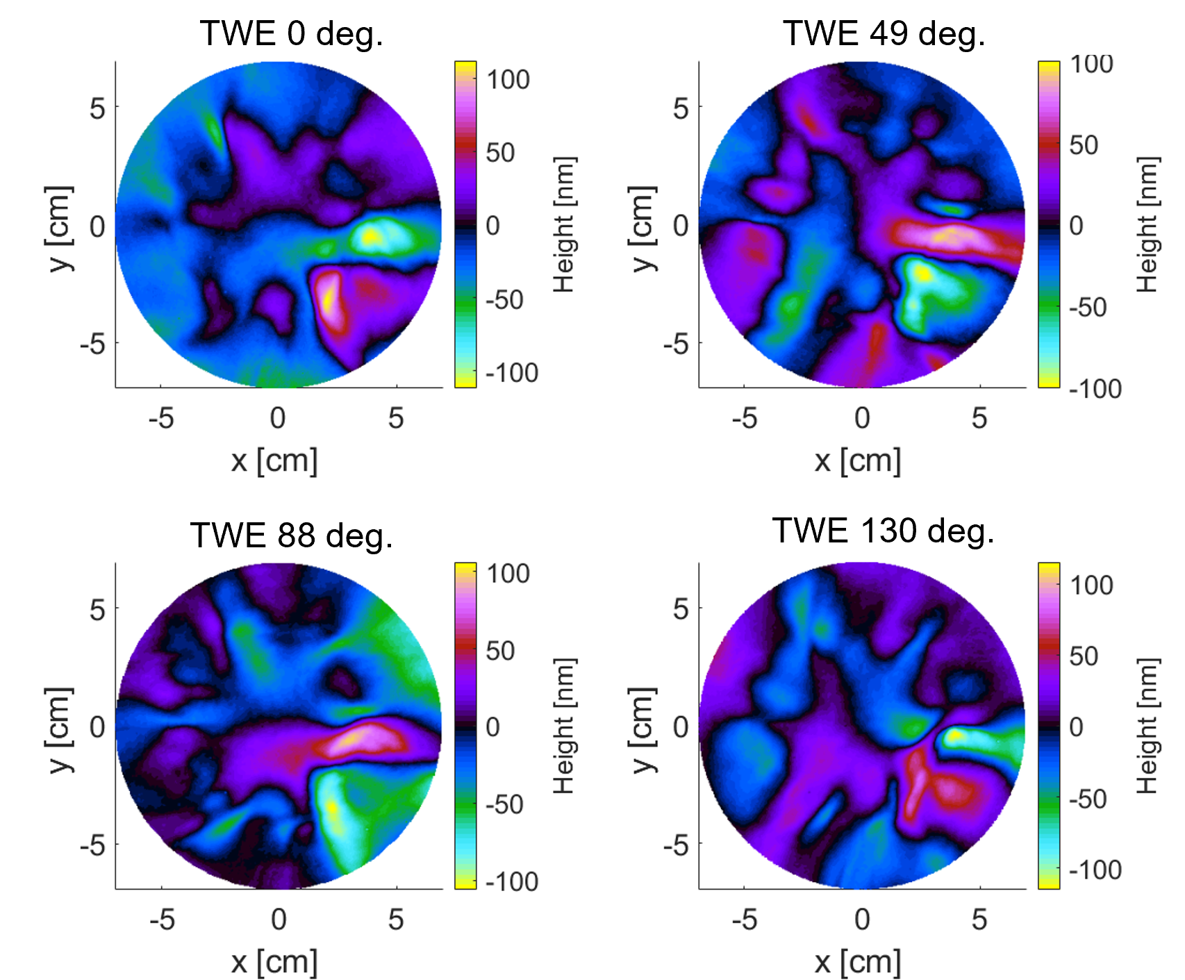
Figure 3: TWE maps of KAGRA’s current ITMY within the 140 mm aperture measured with linearly polarized light with different $\theta$.

The sapphire ITMs have been installed in KAGRA and directly birefringence mapping is impossible. Characterization of the current sapphire test masses has been studied in [31]. TWE maps of ITMs were measured several times with linearly polarized light by rotating the sample at different angles, which is equivalent with measurements by rotating the input polarization. TWE maps were supposed to be measured at 0^∘, 45^∘, 90^∘ and 135^∘. Methods described in Section II have a rigid requirement on the angular control. However, the measurements in [31] were not optimized for birefringence characterization. So, the rotation angle were not precisely controlled at that time. By comparing locations of the markers on the edge of the mirror in different maps, we were able to recover the real rotation angle (shown in Figure 3). One should notice that TWEs of KAGRA current ITMs measured with linearly polarized light are almost one-order of magnitude larger than specifications, because the vendor used circularly polarized light for ion beam figuring during polishing process. It can be seen from Figure 3, the 0^∘ map and the 88^∘ map have almost opposite values (also works for 49^∘ and 130^∘ maps). If summing two maps together, one can derive the TWE for circularly polarized light, which has very small residuals.

III.2 Constructing birefringence maps from TWE

The biggest challenge for birefringence characterizations of KAGRA’s current ITMs comes from the fact that previously TWE measurement setup was not optimized for birefringence study. According to Equation 20 in Section II.3, in order to extract birefringence information, we need subtractions of two pairs of TWE maps and then take the division. In typical Fizeau interferometer measurements, low order effects like the piston and tilt of the surface are not measured. When doing measurements with different $\theta$, the distance and alignment between the sample and reference mirror have changed after rotating the sample. This means that the subtraction of two maps will contain unknown piston and tilt. The numerator and denominator in Equation 20 containing these unknown terms will give wrong birefringence information.

The center of the map also changes after rotating the sample. But we found the decentering is very small (less than 2 mm) and its effect can be negligible when compared with effects from piston and tilt. In addition, we found astigmatisms in original TWE maps. The left plot in Figure 4 shows a TWE map after removing the curvature. A clear astigmatism term can be seen from the map, which is plotted in the right. We found the rotation of this astigmatism does not change when rotating the sample. So, we think the astigmatism comes from the gravity induced deformation of the sample and the astigmatism of the reference mirror used for the Fizeau interferometer. The astigmatism is removed for each TWE map individually.

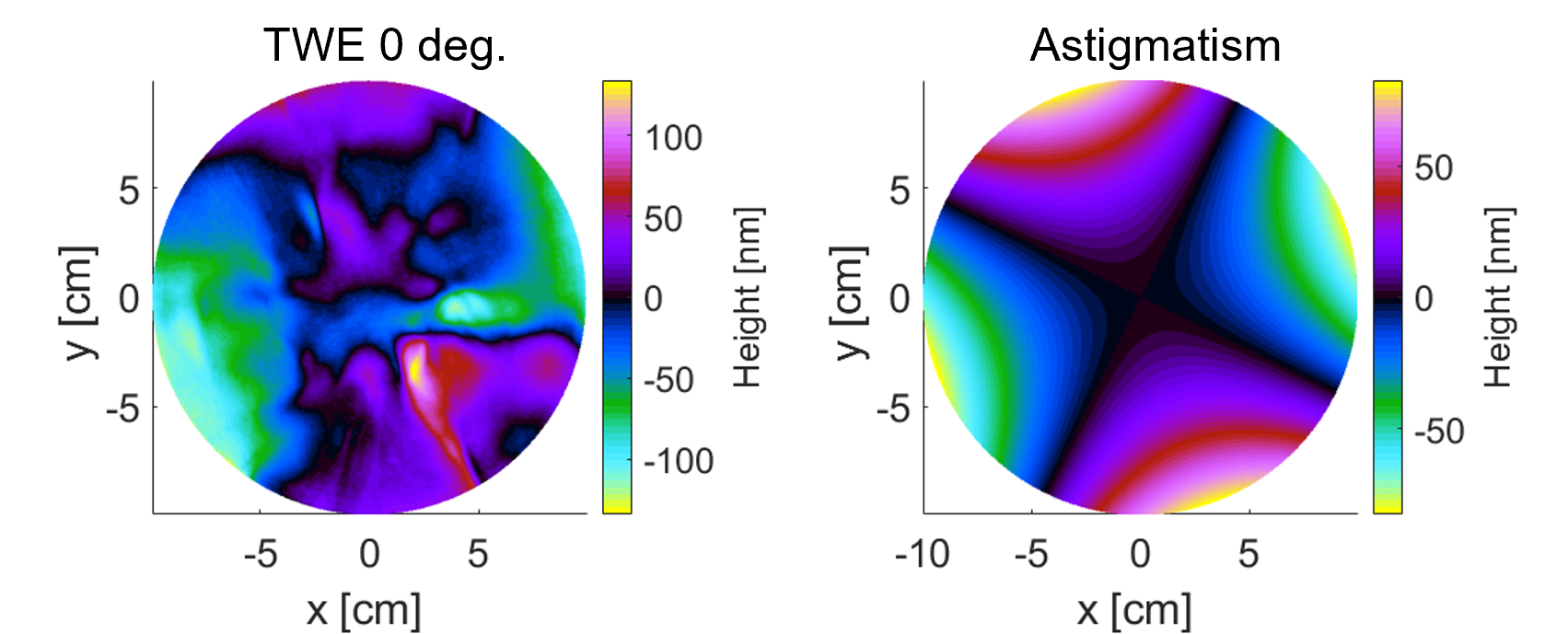
Figure 4: Raw TWE map containing astigmatism which mainly comes from deformation due to gravity. As it is not exactly in the vertical direction, we think the surface of the reference sphere used in the Fizeau interferometer is slightly ellipsoidal. After removing the astigmatism, the TWE is shown in the top left plot in Figure 3.

From Equation 21, $\theta$ is wrapped in the range of ($-45^{\circ}$, $45^{\circ}$) due to $\arctan$ function and we need to unwrap the data. Phase unwrapping techniques are widely used in optical metrology and interferometry [32, 33]. In our case, the problem of unknown piston and tilt is that it will give wrong $\theta$ and cause failure of unwrapping. There are algorithms improving phase unwrapping robustness again noise [34, 35, 36, 37]. Most of these methods require the noise to be small compared with the phase change. But the unmeasured piston and tilt in our TWE map can be large. As we take the division of two subtractions, the error will be further amplified when the denominator in Equation 20 is close to zero. The left plot in Figure 5 shows our initially derived $\theta$. The unwrapping algorithm cannot work properly for such kind of map (shown in the right). This results in that the unwrapped surface is discontinuous. The algorithm used in this paper is according to [38, 39].

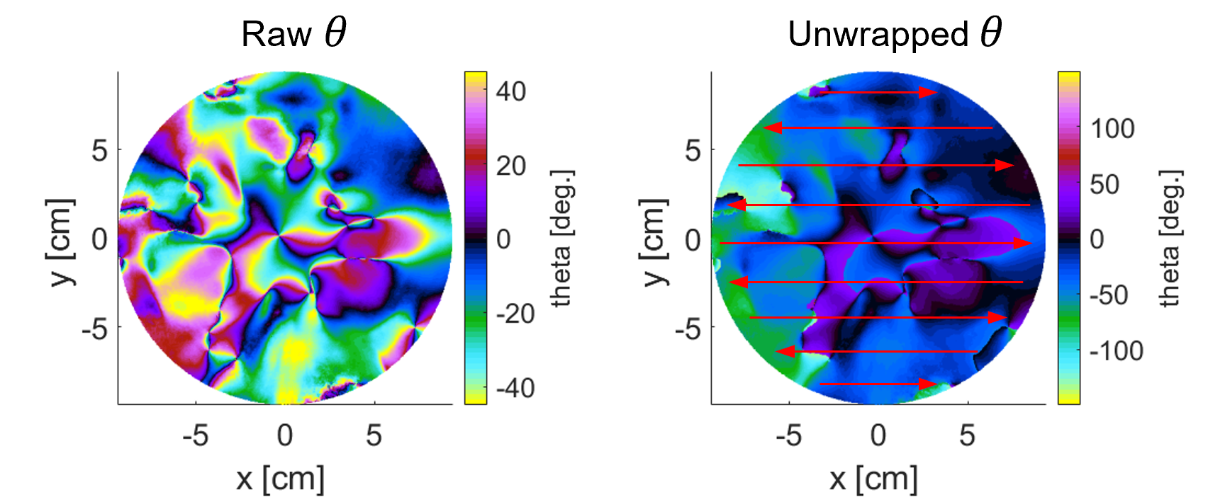
Figure 5: The left plot shows initially derived $\theta$ map according to Equation 20. Unknown piston and tilt will give wrong $\theta$ and cause failure of unwrapping shown in the right where the unwrapped surface is discontinuous. When performing parameter search for pistons, the 2D matrix is expended to 1D vector along the arrow direction. Each arrow represents a row in the 477$\times$477 data matrix.

In order to recover the correct $\theta$, we perform parameter search for piston terms in the numerator and denominator in Equation 20 (while tilt terms are removed individually for each TWE map and ignored here). This yields

$$r=\frac{\psi(\eta_{1})-\psi(\eta_{2})+p_{1}}{\psi(\eta_{3})-\psi(\eta_{4})+p_{2}},$$ (23)

where $p_{1}$ and $p_{2}$ are the missing piston terms. For each pair of $p_{1}$ and $p_{2}$ values, we unwrap the derived raw $\theta$ map. Here, we assume the unmeasured pistons are the main cause for the failure of unwrapping. The two-dimensional unwrapped map is then expended to one-dimensional data along the arrow direction shown in the right in Figure 5. If the unwrapped map is a continuous surface, the one-dimensional data should be a continuous curve. So the overall continuity factor of the map can be simply described by

$$\mathcal{C}=\sum_{k=1}^{n}(\epsilon_{k+1}-\epsilon_{k})^{2},$$ (24)

where $\epsilon_{k}$ is the TWE value at each point of the one-dimensional data and $n$ is the total number of the data. Lower value of $\mathcal{C}$ means a smoother surface while higher value of $\mathcal{C}$ means more value jumps over the surface (see the right plot in Figure 5). Continuity factors of ITMX and ITMY are shown in the right in Figure 6. For each pair of $p_{1}$ and $p_{2}$, $\theta$ and $\alpha_{-}$ can be derived. Then we calculate the cross-coupling term $E_{\mathrm{p}}=-i\sin\alpha_{-}\sin 2\theta$ in Equation 2. This gives the field of linearly polarized light in perpendicular direction with the input polarization. It’s beam shape is shown in the left in Figure 6 with different piston values.

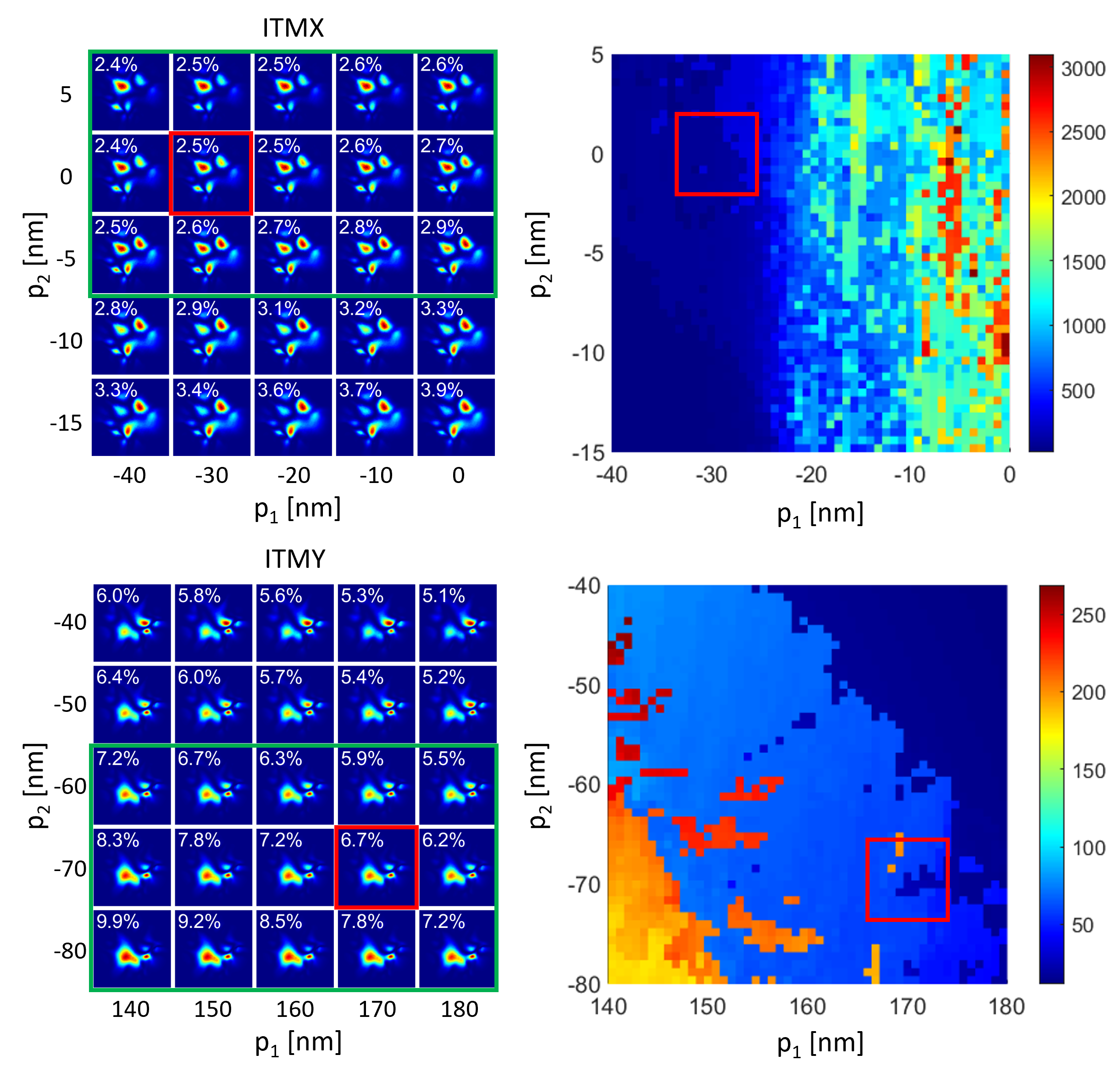
Figure 6: Parameter scan for piston term for ITMX (top) and ITMY (bottom). Plots in the left are single-bounce reflected (passing through the mirror substrate twice) beam shapes in p-polarization (the input is pure s-polarization) with different pistons applied to subtractions of TWEs. Numbers in white are the ratio percentage of beam power in p-polarization over the total input power. Plots in the right are continuity factors of $\theta$ map after unwrapping. It can be seen that $p_{1}$ mainly influence the continuity factor while $p_{2}$ determines the beam shape and power. We search for the correct pistons by eye where continuity factors are small and beam shapes match with measurements shown in Figure 8. We think the beam shape shown in red square gives the best estimation as a consideration of continuity factor and measured beam shape. But actually beams in the green area all have similar shapes with power varying a lot.

III.3 Comparison with in-situ measurements

We have performed birefringence measurements for the sapphire ITMs in KAGRA. A simplified schematic of KAGRA configuration is shown in Figure 7. The laser after the Faraday Isolator is in pure s-polarization. The Power Recycling Mirror (PRM), Signal Recycling Mirror (SRM) and End Test Masses (ETMX and ETMY) are all misaligned so that the beam is reflected back only by ITMs. The plot shows the birefringence measurement for ITMX where ITMY is misaligned. Coatings of the beam splitter (BS) are optimized for s-polarization with a 50%:50% ratio for reflection and transmission at 45^∘ incidence. The ratio for p-polarization is 20%:80% according to the coating design. Since there are no direct measurements for p-polarization, practical reflection and transmission may be different from design values. The reflected beams from ITMs are measured at POP and POS ports. There are photodetectors (PD) and cameras for both s-polarization and p-polarization at POP, while there are only photodetectors at POS.

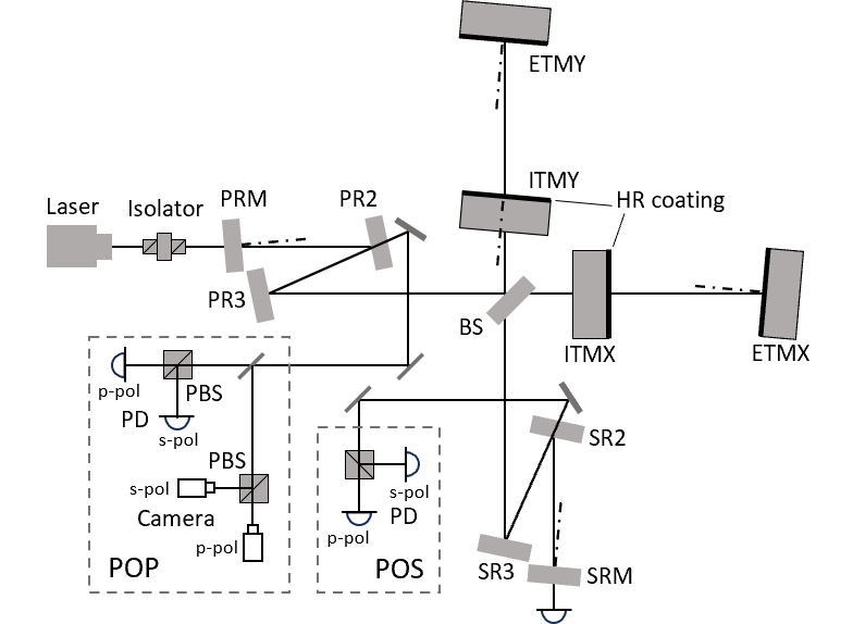
Figure 7: Simplified schematic of KAGRA configuration.

Table 1: Comparison between the measured beam power in p-polarization at POP and POS ports with calculations from $\theta$ and $\alpha_{-}$ maps. Numbers are percentages of the p-polarization power among total power reflected from ITMX or ITMY.

	POP	POS	Calculation
ITMX	$(3.65\pm 0.02)\%$	$(4.98\pm 0.01)\%$	2.5%
ITMY	$(8.07\pm 0.04)\%$	$(11.13\pm 0.02)\%$	6.7%

The measured beam power in p-polarization (as a percentage of the total reflected power) is shown in Table 1, where the effect of unbalanced reflection and transmission of the BS for p-polarization is calibrated (according to coating design values). In principle, the measured beam power content in p-polarization should be the same for POP and POS ports. But in our measurements they are different from each other. We think one reason could be that the practical reflection and transmission of the BS for p-polarization deviate from design. Another reason could be due to the clipping and ghost beam. When the measurement was done, gate valves were added to vacuum tubes whose diameters are just slightly bigger than the beam size. We also found there were a lot of ghost and scattering beams at POP and POS. Though we dumped most of them, there may be still some left and seen by the photodetectors.

Measured beam shapes are shown in the right in Figure 8. By comparing our calculated beam shapes from the previous section with practical measurements, we can find the correct pair of $p_{1}$ and $p_{2}$ by eye which gives both low continuity factor and good agreement with measured beam shapes (see Figure 6). The beam power in p-polarization are then calculated (values are shown in Table 1) with the most suitable pair of $p_{1}$ and $p_{2}$ (marked with red square in Figure 6). The estimated beam power from our maps is smaller than measurements. We think one of the reason is that the unknown tilt term in the measured TWE maps will influence the beam power. By adding tilt influences in the parameter scan, it is possible to increase the calculated power in p-polarization while keeping the beam shape unchanged (or changed by little). In this paper, we don’t perform the full parameter scan for tilt, since the purpose of this paper is to show the feasibility of the method of extracting birefringence information from TWE measurements. An example of the influence of tilt is presented in the Appendix LABEL:app:_tilt.

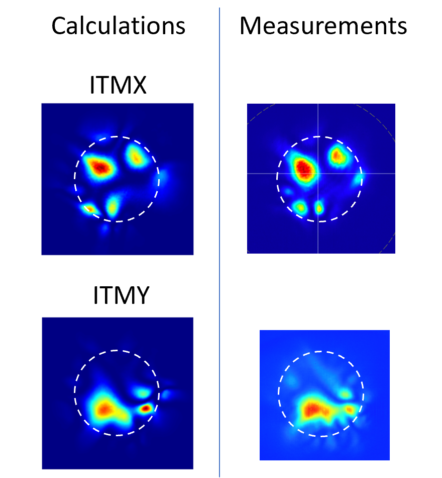
Figure 8: Comparison between calculated p-polarization beam shape and KAGRA measurements. Dashed circles in white represent the Gaussian beam diameter.

Another factor that can affect our estimated power is the beam spot position on the mirror. The beam spots on ITMs in KAGRA are not exactly in the center but a couple of centimeters away where the power recycling gain and arm transmission power are higher, which is probably due to the homogeneous birefringence effect. Figure 9 shows our estimation how much the beam power in p-polarization will change when the beam is miscentered.

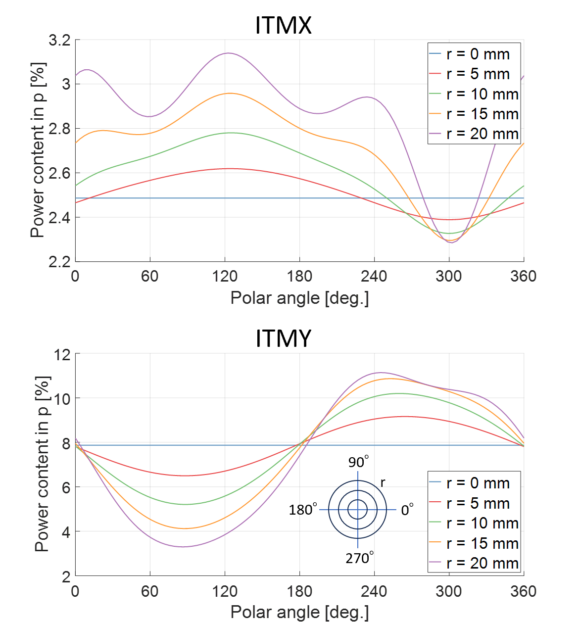
Figure 9: Power of p-polarization when the beam spot is moved away from the mirror center. The x-axis represents the direction of the decenter and $r$ is the distance between the beam spot center and mirror center. Birefringence effect gets smaller when moving the beam towards southeast on ITMX and towards north on ITMY, which can also be seen from Figure 8.

The derived $\theta$ and $\alpha_{-}$ maps for ITMX and ITMY are shown in Figure 10. From these maps, we can see the birefringence in KAGRA’s current ITMs are quite inhomogeneous. If we compare these maps with the beam shape in p-polarization shown in Figure 8, it can be found the beam shape is mainly determined by the shape of $\theta$ map. This is because $\alpha_{-}$ is small in our case. The $\sin 2\theta$ term plays a more important part than $\sin\alpha_{-}$ in the amplitude of the field in p-polarization from Equation 7.

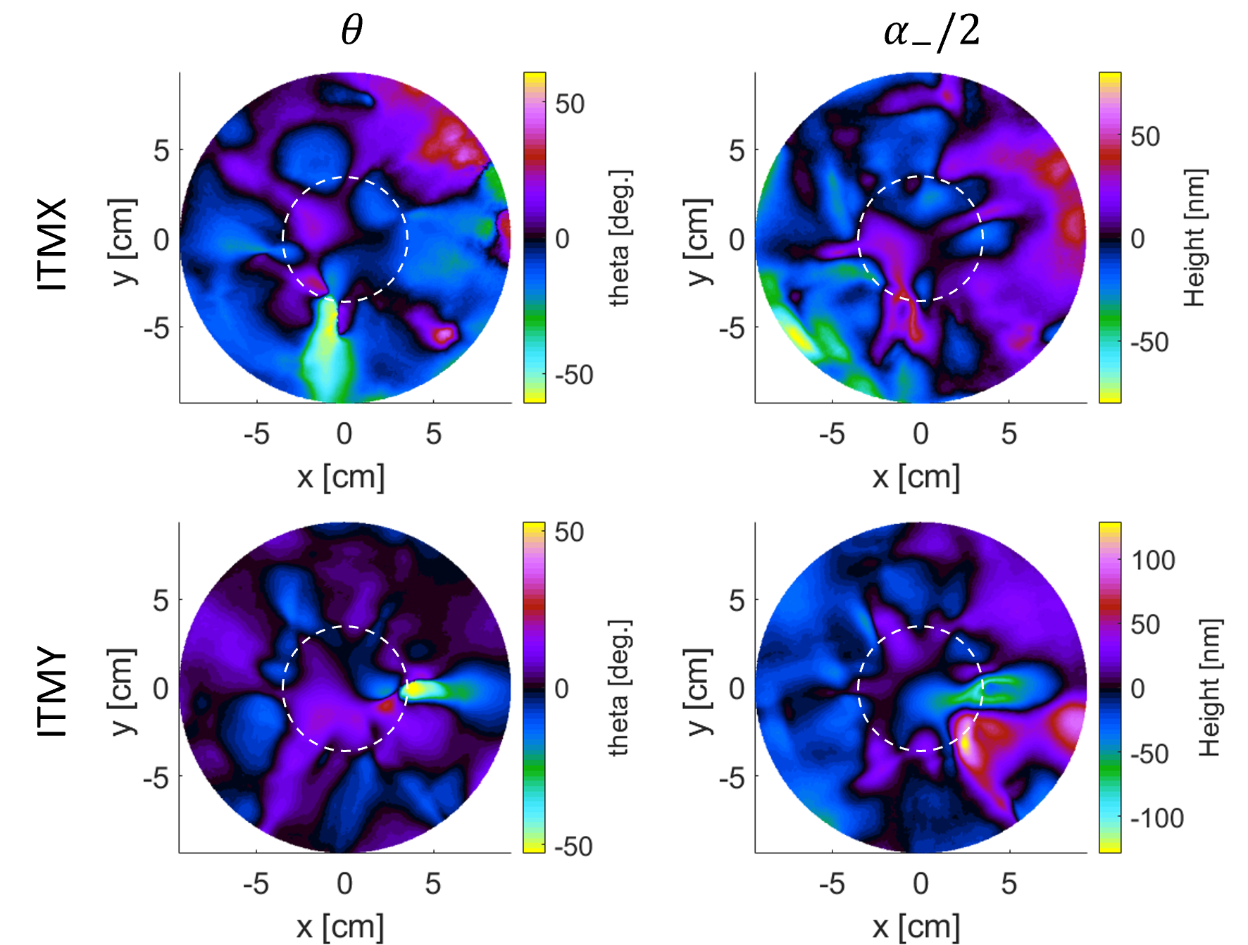
Figure 10: Calibrated $\theta$ and $\alpha_{-}$ maps for ITMX and ITMY. Dashed circles represent the laser beam diameter on mirrors. The plots shown here are the one-way differential phase $\alpha_{-}/2$. The unit of $\alpha_{-}$ is nanometer and the laser wavelength 1064 nm corresponds to a radian of $2\pi$.

As discussed above, a good knowledge of piston and tilt in TWE measurements, as well as the location of the beam spot are necessary in order to precisely estimate the birefringence effect. For more accurate characterizations, the previous setup requires improvements and optimizations for birefringence study.

IV Conclusion and discussion

We have established a method to reconstruct the 2D birefringence information of current KAGRA’s sapphire ITMs from TWE measurements. By combining several TWE measurements with a Fizeau interferometer using linearly polarization in different rotation angles, we are able to successfully construct the birefringence map over a 200 mm area in diameter. Our estimated beam shape for single bounce reflected field in orthogonal polarization shows a good match with in-situ measurements in KAGRA.

It is worth to point out that these TWE measurements were not intended for birefringence characterizations. More accurate reconstruction requires improvements of the previous setup which should target for birefringence study. One possible improvement could be enabling the control of the polarization rotation angle of the input laser in the Fizeau interferometer rather than rotating the tested mirror, as this will remove the influence of the low order (piston, tilt and astigmatism caused by deformation due to gravity) error term in TWE. For future gravitational wave detectors, since most potential materials feasible for cryogenic operation are birefringent, birefringence has become an important parameter for their core optics. This technique of birefringence mapping described in this paper is fast and simple. It can be crucial for future detectors where larger test masses are used. In addition, specifications of mirror birefringence requires a full understanding of how the birefringence affects the performance of the interferometer. The derived birefringence map in this paper can be used to study the effects of inhomogeneous birefringence in future detectors and help us to gain insights of this knowledge.

Appendix A Effective Jones matrix of a non-uniform medium along the optical axis

In Section II, we assumed that the transmission of light through a substrate can be described by a single Jones matrix (Equation 2). At a glance, this seems to imply that we also assume the birefringence properties ($\theta$, $n_{e}$ and $n_{o}$) to be constant along the depth of the substrate. However, this assumption does not hold for most real substrates. For the sapphire substrates of the KAGRA mirrors, for example, the fluctuation of birefringence is supposed to come from local mis-alignment of crystal axes, possibly caused by residual internal stress, lattice defects and so on. Then, the birefringence properties must vary not only laterally but also along the depth of the substrate. Then a question arises: can we use a single Jones matrix to describe a complex birefringent medium? In this section, we will address this question.

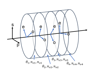
Figure 11: Splitting a substrate into thin slices.

We start from splitting a thick substrate into thin slices as shown in Figure 11. Each slice is thin enough that the birefringence properties can be regarded as constant within it. Transmission of light through such a thin slice can be described by a single Jones matrix of the form in Equation 2.

As we make the slice infinitesimally thin, $\alpha_{-}$ becomes also infinitesimally small. From Equation 2, we can expand the Jones matrix with $\alpha_{-}$ and leave only its first order terms (the common phase term $\alpha_{+}$ is omitted here),

$$M =\begin{pmatrix}\cos\alpha_{-}+i\cos 2\theta\sin\alpha_{-}&-i\sin 2\theta\sin\alpha_{-}\\ -i\sin 2\theta\sin\alpha_{-}&\cos\alpha_{-}-i\cos 2\theta\sin\alpha_{-}\end{pmatrix}$$ (25)

$$\sim\begin{pmatrix}1+i\cos 2\theta\cdot\alpha_{-}&-i\sin 2\theta\cdot\alpha_{-}\\ -i\sin 2\theta\cdot\alpha_{-}&1-i\cos 2\theta\cdot\alpha_{-}\end{pmatrix}.$$ (26)

The next step is to consider the transmission of light through two consecutive slices having different Jones matrices:

$$M_{1} =\begin{pmatrix}1+i\cos 2\theta_{1}\cdot\alpha_{1}&-i\sin 2\theta_{1}\cdot\alpha_{1}\\ -i\sin 2\theta_{1}\cdot\alpha_{1}&1-i\cos 2\theta_{1}\cdot\alpha_{1}\end{pmatrix},$$ (27)

$$M_{2} =\begin{pmatrix}1+i\cos 2\theta_{2}\cdot\alpha_{2}&-i\sin 2\theta_{2}\cdot\alpha_{2}\\ -i\sin 2\theta_{2}\cdot\alpha_{2}&1-i\cos 2\theta_{2}\cdot\alpha_{2}\end{pmatrix}.$$ (28)

Such a process can be described by the multiplication of the two Jones matrices,

$$M_{12}=M_{2}\cdot M_{1}=\begin{pmatrix}1+i\left(\cos 2\theta_{1}\cdot\alpha_{1}+\cos 2\theta_{2}\cdot\alpha_{2}\right)&-i\left(\sin 2\theta_{1}\cdot\alpha_{1}+\sin 2\theta_{2}\cdot\alpha_{2}\right)\\ -i\left(\sin 2\theta_{1}\cdot\alpha_{1}+\sin 2\theta_{2}\cdot\alpha_{2}\right)&1-i\left(\cos 2\theta_{1}\cdot\alpha_{1}+\cos 2\theta_{2}\cdot\alpha_{2}\right)\end{pmatrix}.$$ (29)

By comparing Equation 29 and Equation 26, we need to find $\alpha_{\mathrm{e}}$ and $\theta_{\mathrm{e}}$ which satisfy the following conditions,

$$\alpha_{\mathrm{e}}\cos 2\theta_{\mathrm{e}} =\cos 2\theta_{1}\cdot\alpha_{1}+\cos 2\theta_{2}\cdot\alpha_{2}$$ (30)

$$\alpha_{\mathrm{e}}\sin 2\theta_{\mathrm{e}} =\sin 2\theta_{1}\cdot\alpha_{1}+\sin 2\theta_{2}\cdot\alpha_{2}.$$ (31)

Finding such a combination of $\alpha_{\mathrm{e}}$ and $\theta_{\mathrm{e}}$ is always possible. Then we can express $M_{12}$ using these parameters as,

$$M_{12}=\begin{pmatrix}1+i\cos 2\theta_{\mathrm{e}}\cdot\alpha_{\mathrm{e}}&-i\sin 2\theta_{\mathrm{e}}\cdot\alpha_{\mathrm{e}}\\ -i\sin 2\theta_{\mathrm{e}}\cdot\alpha_{\mathrm{e}}&1-i\cos 2\theta_{\mathrm{e}}\cdot\alpha_{\mathrm{e}}\end{pmatrix}.$$ (32)

This is an effective Jones matrix for the transmission of two consecutive thin slices. By repeating this process, we can always find a single Jones matrix of the form shown in Equation 2 representing the transmission of a thicker substrate. Therefore, the use of Equation 2 for the analysis of an inhomogeneous thick substrate is justified.

Appendix B Influence of tilt of TWE maps on the estimation of beam shape and beam power

In Section III.2, we show that the piston, which is usually ignored in an interferometric measurement with Fizeau interferometers, however, is an important factor in birefringence measurements with the method described in this paper. The tilt, also ignored in TWE measurements, has a similar effect. In this section, we give an example of its influence to our birefringence characterizations.

The tilt of a surface can be described by a combination of the first-order Zernike polynomials $Z_{1}^{-1}$ and $Z_{1}^{1}$ (shwon in Figure 12). Thus we need to add two degrees of freedom of tilt for nominator and denominator respectively in Equation 23 and this ends up with four more degrees of freedom ($a$, $b$, $c$ and $d$) for parameter scan, which yields

$$r=\frac{\psi(\eta_{1})-\psi(\eta_{2})+p_{1}+aZ_{1}^{-1}+bZ_{1}^{1}}{\psi(\eta_{3})-\psi(\eta_{4})+p_{2}+cZ_{1}^{-1}+dZ_{1}^{1}}.$$ (33)

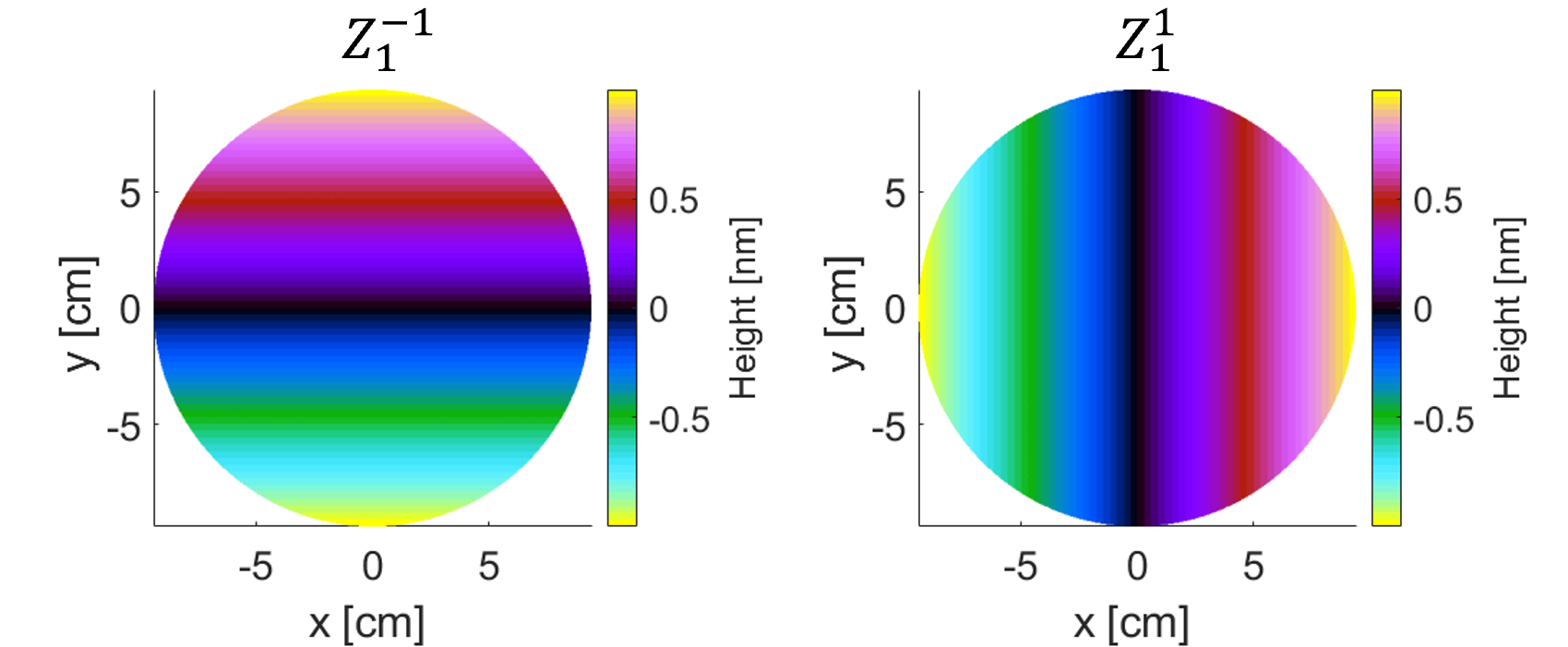
Figure 12: The first order coefficients of Zernike polynomials. Any tilt of a surface can be described with a combination of them with different amplitudes.

According to Figure 6, the change in the nominator in Equation 33 mainly influences the continuity factor, while the change in the denominator has a larger effect on the beam shape and power. Here, we set $a=b=0$ to see the influence of tilt on beam shape and power. Pistons $p_{1}$ and $p_{2}$ are fixed according to values giving results in red squares in Figure 6. Figure 13 shows the change of beam shape and power when we apply different amount of tilt to the denominator. The results labeled in red squares show a good match with birefringence measurements at POP in terms of both beam shape and beam power in p-polarization.

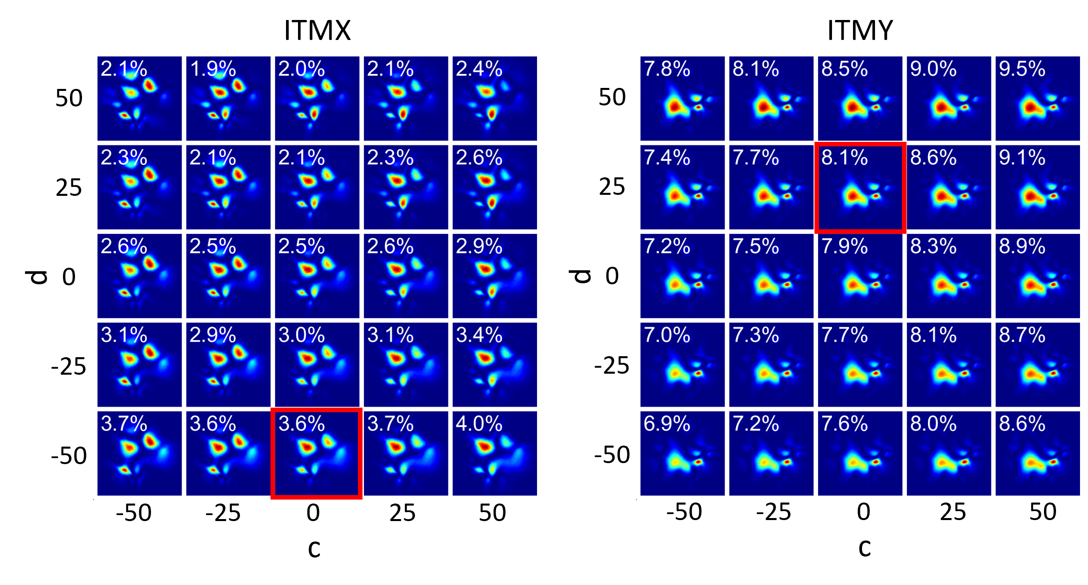
Figure 13: An example of parameter scan showing the change of beam shape and power in p-polarization with different magnitude of tilt.

References

- Flaminio [2014] R. Flaminio, Thermal noise in laser interferometer gravitational wave detectors, in Advanced Interferometers and the Search for Gravitational Waves: Lectures from the First VESF School on Advanced Detectors for Gravitational Waves, edited by M. Bassan (Springer International Publishing, Cham, 2014) pp. 225–249.
- Nawrodt et al. [2011] R. Nawrodt, S. Rowan, J. Hough, M. Punturo, F. Ricci, and J.-Y. Vinet, General Relativity and Gravitation 43, 593 (2011).
- Adhikari et al. [2020] R. X. Adhikari, K. Arai, A. F. Brooks, C. Wipf, O. Aguiar, P. Altin, B. Barr, L. Barsotti, R. Bassiri, A. Bell, G. Billingsley, R. Birney, D. Blair, E. Bonilla, J. Briggs, D. D. Brown, R. Byer, H. Cao, M. Constancio, S. Cooper, T. Corbitt, D. Coyne, A. Cumming, E. Daw, R. deRosa, G. Eddolls, J. Eichholz, M. Evans, M. Fejer, E. C. Ferreira, A. Freise, V. V. Frolov, S. Gras, A. Green, H. Grote, E. Gustafson, E. D. Hall, G. Hammond, J. Harms, G. Harry, K. Haughian, D. Heinert, M. Heintze, F. Hellman, J. Hennig, M. Hennig, S. Hild, J. Hough, W. Johnson, B. Kamai, D. Kapasi, K. Komori, D. Koptsov, M. Korobko, W. Z. Korth, K. Kuns, B. Lantz, S. Leavey, F. Magana-Sandoval, G. Mansell, A. Markosyan, A. Markowitz, I. Martin, R. Martin, D. Martynov, D. E. McClelland, G. McGhee, T. McRae, J. Mills, V. Mitrofanov, M. Molina-Ruiz, C. Mow-Lowry, J. Munch, P. Murray, S. Ng, M. A. Okada, D. J. Ottaway, L. Prokhorov, V. Quetschke, S. Reid, D. Reitze, J. Richardson, R. Robie, I. Romero-Shaw, R. Route, S. Rowan, R. Schnabel, M. Schneewind, F. Seifert, D. Shaddock, B. Shapiro, D. Shoemaker, A. S. Silva, B. Slagmolen, J. Smith, N. Smith, J. Steinlechner, K. Strain, D. Taira, S. Tait, D. Tanner, Z. Tornasi, C. Torrie, M. V. Veggel, J. Vanheijningen, P. Veitch, A. Wade, G. Wallace, R. Ward, R. Weiss, P. Wessels, B. Willke, H. Yamamoto, M. J. Yap, and C. Zhao, Classical and Quantum Gravity 37, 165003 (2020).
- Punturo et al. [2010] M. Punturo, M. Abernathy, F. Acernese, B. Allen, N. Andersson, K. Arun, F. Barone, B. Barr, M. Barsuglia, M. Beker, N. Beveridge, S. Birindelli, S. Bose, L. Bosi, S. Braccini, C. Bradaschia, T. Bulik, E. Calloni, G. Cella, E. C. Mottin, S. Chelkowski, A. Chincarini, J. Clark, E. Coccia, C. Colacino, J. Colas, A. Cumming, L. Cunningham, E. Cuoco, S. Danilishin, K. Danzmann, G. D. Luca, R. D. Salvo, T. Dent, R. D. Rosa, L. D. Fiore, A. D. Virgilio, M. Doets, V. Fafone, P. Falferi, R. Flaminio, J. Franc, F. Frasconi, A. Freise, P. Fulda, J. Gair, G. Gemme, A. Gennai, A. Giazotto, K. Glampedakis, M. Granata, H. Grote, G. Guidi, G. Hammond, M. Hannam, J. Harms, D. Heinert, M. Hendry, I. Heng, E. Hennes, S. Hild, J. Hough, S. Husa, S. Huttner, G. Jones, F. Khalili, K. Kokeyama, K. Kokkotas, B. Krishnan, M. Lorenzini, H. Lück, E. Majorana, I. Mandel, V. Mandic, I. Martin, C. Michel, Y. Minenkov, N. Morgado, S. Mosca, B. Mours, H. Müller–Ebhardt, P. Murray, R. Nawrodt, J. Nelson, R. Oshaughnessy, C. D. Ott, C. Palomba, A. Paoli, G. Parguez, A. Pasqualetti, R. Passaquieti, D. Passuello, L. Pinard, R. Poggiani, P. Popolizio, M. Prato, P. Puppo, D. Rabeling, P. Rapagnani, J. Read, T. Regimbau, H. Rehbein, S. Reid, L. Rezzolla, F. Ricci, F. Richard, A. Rocchi, S. Rowan, A. Rüdiger, B. Sassolas, B. Sathyaprakash, R. Schnabel, C. Schwarz, P. Seidel, A. Sintes, K. Somiya, F. Speirits, K. Strain, S. Strigin, P. Sutton, S. Tarabrin, A. Thüring, J. van den Brand, C. van Leewen, M. van Veggel, C. van den Broeck, A. Vecchio, J. Veitch, F. Vetrano, A. Vicere, S. Vyatchanin, B. Willke, G. Woan, P. Wolfango, and K. Yamamoto, Classical and Quantum Gravity 27, 194002 (2010).
- ET steering committee [2020] ET steering committee, ET design report update 2020, Tech. Rep. ET-0007B-20 (2020).
- Hall [2022] E. D. Hall, Galaxies 10, 90 (2022).
- Akutsu et al. [2021] T. Akutsu, M. Ando, K. Arai, Y. Arai, S. Araki, A. Araya, N. Aritomi, Y. Aso, S. Bae, Y. Bae, et al., Progress of Theoretical and Experimental Physics 2021, 05A101 (2021).
- Michimura et al. [2020] Y. Michimura, K. Komori, Y. Enomoto, K. Nagano, A. Nishizawa, E. Hirose, M. Leonardi, E. Capocasa, N. Aritomi, Y. Zhao, R. Flaminio, T. Ushiba, T. Yamada, L.-W. Wei, H. Takeda, S. Tanioka, M. Ando, K. Yamamoto, K. Hayama, S. Haino, and K. Somiya, Phys. Rev. D 102, 022008 (2020).
- Somiya [2012] K. Somiya, Classical and Quantum Gravity 29, 124007 (2012).
- Aso et al. [2013] Y. Aso, Y. Michimura, K. Somiya, M. Ando, O. Miyakawa, T. Sekiguchi, D. Tatsumi, and H. Yamamoto (The KAGRA Collaboration), Phys. Rev. D 88, 043007 (2013).
- Hirose et al. [2014] E. Hirose, D. Bajuk, G. Billingsley, T. Kajita, B. Kestner, N. Mio, M. Ohashi, B. Reichman, H. Yamamoto, and L. Zhang, Phys. Rev. D 89, 062003 (2014).
- Uchiyama et al. [1999] T. Uchiyama, T. Tomaru, M. Tobar, D. Tatsumi, S. Miyoki, M. Ohashi, K. Kuroda, T. Suzuki, N. Sato, T. Haruyama, A. Yamamoto, and T. Shintomi, Physics Letters A 261, 5 (1999).
- Tomaru et al. [2002] T. Tomaru, T. Suzuki, S. Miyoki, T. Uchiyama, C. T. Taylor, A. Yamamoto, T. Shintomi, M. Ohashi, and K. Kuroda, Classical and Quantum Gravity 19, 2045 (2002).
- Krüger et al. [2015] C. Krüger, D. Heinert, A. Khalaidovski, J. Steinlechner, R. Nawrodt, R. Schnabel, and H. Lück, Classical and Quantum Gravity 33, 015012 (2015).
- Jaberian Hamedan et al. [2023] V. Jaberian Hamedan, A. Adam, C. Blair, L. Ju, and C. Zhao, Applied Physics Letters 122, 064101 (2023).
- Winkler et al. [2021] G. Winkler, L. W. Perner, G.-W. Truong, G. Zhao, D. Bachmann, A. S. Mayer, J. Fellinger, D. Follman, P. Heu, C. Deutsch, D. M. Bailey, H. Peelaers, S. Puchegger, A. J. Fleisher, G. D. Cole, and O. H. Heckl, Optica 8, 686 (2021).
- Tanioka et al. [2023] S. Tanioka, D. Vander-Hyde, G. D. Cole, S. D. Penn, and S. W. Ballmer, Phys. Rev. D 107, 022003 (2023).
- Somiya et al. [2019] K. Somiya, E. Hirose, and Y. Michimura, Phys. Rev. D 100, 082005 (2019).
- Michimura et al. [2024] Y. Michimura, H. Wang, F. Salces-Carcoba, C. Wipf, A. Brooks, K. Arai, and R. X. Adhikari, Phys. Rev. D 109, 022009 (2024).
- Pastrnak and Vedam [1971] J. Pastrnak and K. Vedam, Phys. Rev. B 3, 2567 (1971).
- Shribak and Oldenbourg [2003] M. Shribak and R. Oldenbourg, Appl. Opt. 42, 3009 (2003).
- Onuma and Otani [2014] T. Onuma and Y. Otani, Optics Communications 315, 69 (2014).
- de Villèle and Loriette [2000] G. de Villèle and V. Loriette, Appl. Opt. 39, 3864 (2000).
- Chu et al. [2002] T. Chu, M. Yamada, J. Donecker, M. Rossberg, V. Alex, and H. Riemann, Materials Science and Engineering: B 91-92, 174 (2002).
- Tokunari et al. [2006] M. Tokunari, H. Hayakawa, K. Yamamoto, T. Uchiyama, S. Miyoki, M. Ohashi, and K. Kuroda, Journal of Physics: Conference Series 32, 432 (2006).
- Zeidler et al. [2023] S. Zeidler, M. Eisenmann, M. Bazzan, P. Li, and M. Leonardi, Scientific Reports 13, 21393 (2023).
- Noguchi et al. [1992] M. Noguchi, T. Ishikawa, M. Ohno, and S. Tachihara, Intl Symp on Optical Fabrication, Testing, and Surface Evaluation, Proceedings of SPIE 1720, 367 (1992).
- Otani et al. [1994] Y. Otani, T. Shimada, T. Yoshizawa, and N. Umeda, Optical Engineering 33, 1604 (1994).
- Cochran and Ai [1992] E. R. Cochran and C. Ai, Appl. Opt. 31, 6702 (1992).
- Yariv and Yeh [2007] A. Yariv and P. Yeh, Photonics: optical electronics in modern communications (Oxford university press, 2007).
- Hirose et al. [2020] E. Hirose, G. Billingsley, L. Zhang, H. Yamamoto, L. Pinard, C. Michel, D. Forest, B. Reichman, and M. Gross, Phys. Rev. Appl. 14, 014021 (2020).
- Judge and Bryanston-Cross [1994] T. Judge and P. Bryanston-Cross, Optics and Lasers in Engineering 21, 199 (1994).
- Su and Chen [2004] X. Su and W. Chen, Optics and Lasers in Engineering 42, 245 (2004).
- Cusack et al. [1995] R. Cusack, J. M. Huntley, and H. T. Goldrein, Appl. Opt. 34, 781 (1995).
- Buckland et al. [1995] J. R. Buckland, J. M. Huntley, and S. R. E. Turner, Appl. Opt. 34, 5100 (1995).
- Volkov and Zhu [2003] V. V. Volkov and Y. Zhu, Opt. Lett. 28, 2156 (2003).
- Estrada et al. [2011] J. C. Estrada, M. Servin, and J. A. Quiroga, Opt. Express 19, 5126 (2011).
- Herráez et al. [2002] M. A. Herráez, D. R. Burton, M. J. Lalor, and M. A. Gdeisat, Appl. Opt. 41, 7437 (2002).
- Kasim [2017] M. Kasim, GitHub (2017).