QN-Mixer: A Quasi-Newton MLP-Mixer Model
for Sparse-View CT Reconstruction

Abstract

Inverse problems span across diverse fields. In medical contexts, computed tomography (CT) plays a crucial role in reconstructing a patient’s internal structure, presenting challenges due to artifacts caused by inherently ill-posed inverse problems. Previous research advanced image quality via post-processing and deep unrolling algorithms but faces challenges, such as extended convergence times with ultra-sparse data. Despite enhancements, resulting images often show significant artifacts, limiting their effectiveness for real-world diagnostic applications. We aim to explore deep second-order unrolling algorithms for solving imaging inverse problems, emphasizing their faster convergence and lower time complexity compared to common first-order methods like gradient descent. In this paper, we introduce QN-Mixer, an algorithm based on the quasi-Newton approach. We use learned parameters through the BFGS algorithm and introduce Incept-Mixer, an efficient neural architecture that serves as a non-local regularization term, capturing long-range dependencies within images. To address the computational demands typically associated with quasi-Newton algorithms that require full Hessian matrix computations, we present a memory-efficient alternative. Our approach intelligently downsamples gradient information, significantly reducing computational requirements while maintaining performance. The approach is validated through experiments on the sparse-view CT problem, involving various datasets and scanning protocols, and is compared with post-processing and deep unrolling state-of-the-art approaches. Our method outperforms existing approaches and achieves state-of-the-art performance in terms of SSIM and PSNR, all while reducing the number of unrolling iterations required.

Figure 1: CT Reconstruction with 32 views of State-of-the-Art Methods. Comparative analysis with post-processing and first-order unrolling networks highlights QN-Mixer’s superiority in artifact removal, training time, and data efficiency.

1 Introduction

Computed tomography (CT) is a widely used imaging modality in medical diagnosis and treatment planning, delivering intricate anatomical details of the human body with precision. Despite its success, CT is associated with high radiation doses, which can increase the risk of cancer induction [46]. Adhering to the ALARA principle (As Low As Reasonably Achievable) [34], the medical community emphasizes minimizing radiation exposure to the lowest level necessary for accurate diagnosis. Numerous approaches have been proposed to reduce radiation doses while maintaining image quality. Among these, sparse-view CT emerges as a promising solution, effectively lowering radiation doses by subsampling the projection data, often referred to as the sinogram. Nonetheless, reconstructed images using the well-known Filtered Back Projection (FBP) algorithm [31], suffer from pronounced streaking artifacts (see Fig. 1), which can lead to misdiagnosis. The challenge of effectively reconstructing high-quality CT images from sparse-view data is gaining increasing attention in both the computer vision and medical imaging communities.

With the success of deep learning spanning diverse domains, initial image-domain techniques [5, 17, 54, 23, 25] have been introduced as post-processing tasks on the FBP reconstructed images, exhibiting notable accomplishments in artifact removal and structure preservation. However, the inherent limitations of these methods arise from their constrained receptive fields, leading to challenges in effectively capturing global information and, consequently, sub-optimal results.

To address this limitation, recent advances have seen a shift toward a dual-domain approach [26, 16, 45, 24], where post-processing methods turn to the sinogram domain. In this dual-domain paradigm, deep neural networks are employed to perform interpolation tasks on the sinogram data [22, 14], facilitating more accurate image reconstruction. Despite the significant achievements of post-processing and dual-domain methods, they confront issues of interpretability and performance limitations, especially when working with small datasets and ultra-sparse-view data, as shown in Fig. 1. To tackle these challenges, deep unrolling networks have been introduced [1, 15, 6, 47, 7, 10, 18, 50]. Unrolling networks treat the sparse-view CT reconstruction problem as an optimization task, resulting in a first-order iterative algorithm like gradient descent, which is subsequently unrolled into a deep recurrent neural network in order to learn the optimization parameters and the regularization term. Like post-processing techniques, unrolling networks have been extended to the sinogram domain [48, 52] to perform interpolation task.

Unrolling networks, as referenced in [41, 11, 33], exhibit remarkable performance across diverse domains. However, they suffer from slow convergence and high computational costs, as illustrated in Fig. 1, necessitating the development of more efficient alternatives [13]. More specifically, they confront two main issues: Firstly, they frequently grapple with capturing long-range dependencies due to their dependence on locally-focused regularization terms using CNNs. This limitation results in suboptimal outcomes, particularly evident in tasks such as image reconstruction. Secondly, the escalating computational costs of unrolling methods align with the general trend of increased complexity in modern neural networks. This escalation not only amplifies the required number of iterations due to the algorithm’s iterative nature but also contributes to their high computational demand.

To tackle the aforementioned issues, we introduce a novel second-order unrolling network for sparse-view CT reconstruction. In particular, to enable the learnable regularization term to apprehend long-range interactions within the image, we propose a non-local regularization block termed Incept-Mixer. Drawing inspiration from the multi-layer perceptron mixer [43] and the inception architecture [42], it is created to combine the best features from both sides: capturing long-range interactions from the attention-like mechanism of MLP-Mixer and extracting local invariant features from the inception block. This block facilitates a more precise image reconstruction. Second, to cut down on the computational costs associated with unrolling networks, we propose to decrease the required iterations for convergence by employing second-order optimization methods such as [19, 27]. We introduce a novel unrolling framework named QN-Mixer. Our approach is based on the quasi-Newton method that approximate the Hessian matrix using the Broyden-Fletcher-Goldfarb-Shanno (BFGS) update [12, 9, 53]. Furthermore, we reduce memory usage by working on a projected gradient (latent gradient), preserving performance while reducing the computational cost tied to Hessian matrix approximation. This adaptation enables the construction of a deep unrolling network, showcasing superlinear convergence. Our contributions are summarized as follows:

• We introduce a novel second-order unrolling network coined QN-Mixer where the Hessian matrix is approximated using a latent BFGS algorithm with a deep-net learned regularization term.
  

• We propose Incept-Mixer, a neural architecture acting as a non-local regularization term. Incept-Mixer integrates deep features from inception blocks with MLP-Mixer, enhancing multi-scale information usage and capturing long-range dependencies.
  

• We demonstrate the effectiveness of our proposed method when applied to the sparse-view CT reconstruction problem on an extensive set of experiments and datasets. We show that our method outperforms state-of-the-art methods in terms of quantitative metrics while requiring less iterations than first-order unrolling networks.

2 Related Works

In this section, we present prior work closely related to our paper. We begin by discussing the general framework for unrolling networks in Sec. 2.1, which is based on the gradient descent algorithm. Subsequently, in Sec. 2.2 and Sec. 2.3, we delve into state-of-the-art methods in post-processing and unrolling networks, respectively.

2.1 Background

Inverse Problem Formulation for CT.  Image reconstruction problem in CT can be mathematically formalized as the solution to a linear equation in the form of:

$${\bm{y}}={\bm{A}}{\bm{x}}+\epsilon,$$ (1)

where ${\bm{x}}\in\mathbb{R}^{n}$ is the (unknown) object to reconstruct with $n=h\times w$, ${\bm{y}}\in\mathbb{R}^{m}$ is the data (i.e. sinogram), where $m=n_{v}\times n_{d}$, $n_{v}$ and $n_{d}$ denote the number of projection views and detectors, respectively. ${\bm{A}}\in\mathbb{R}^{n\times m}$ is the forward model (i.e. discrete Radon transform [37]), and $\epsilon\in\mathbb{R}^{m}$ is the system noise. The goal of CT image reconstruction is to recover the (unknown) object, ${\bm{x}}$, from the observed data ${\bm{y}}$. As the problem is ill-posed due to the missing data, the linear system in Eq. 1 becomes underdetermined and may have infinite solutions. Hence, reconstructed images suffer from artifacts, blurring, and noise. To address this issue, iterative reconstruction algorithms are utilized to minimize a regularized objective function with a $L^{2}$ norm constraint:

$$\hat{{\bm{x}}}=\underset{{\bm{x}}}{\operatorname{arg}\,\operatorname{min}}\;J({\bm{x}})=\frac{\lambda}{2}\left\lVert{\bm{A}}{\bm{x}}-{\bm{y}}\right\rVert^{2}_{2}+{\mathcal{R}}({\bm{x}}),$$ (2)

where ${\mathcal{R}}({\bm{x}})$ is the regularization term, balanced with the weight $\lambda$. Those ill-posed problems were initially addressed using optimization techniques, such as the truncated singular value decomposition (SVD) algorithm [39], or iterative approaches like the algebraic reconstruction technique (ART) [4], simultaneous ART (SART) [2], conjugate gradient for least squares (CGLS) [20], and total generalized variation regularization (TGV) [40]. Additionally, techniques such as total variation [44] and Tikhonov regularization [8] can be employed to enhance reconstruction results.

Deep Unrolling Networks.  By assuming that the regularization term in Eq. 2 (i.e. ${\mathcal{R}}$) is differentiable and convex, a simple gradient descent scheme can be applied to solve the optimization problem:

$$\begin{aligned} &{\bm{x}}_{t+1}={\bm{x}}_{t}-\alpha\nabla_{\bm{x}}J({\bm{x}}_{t}),\\ &\text{where}\quad\nabla_{\bm{x}}J({\bm{x}}_{t})=\lambda{\bm{A}}^{\dagger}\left({\bm{A}}{\bm{x}}_{t}-{\bm{y}}\right)+\nabla_{\bm{x}}{\mathcal{R}}({\bm{x}}_{t}).\end{aligned}$$ (3)

Here, $\alpha$ represents the step size (i.e. search step), and ${\bm{A}}^{\dagger}$ is the pseudo-inverse of ${\bm{A}}$.

Previous research [49, 15] has emphasized the limitations of optimization algorithms, such as the manual selection of the regularization term and the optimization hyper-parameters, which can negatively impact their performance, limiting their clinical application. Recent advancements in deep learning techniques have enabled automated parameter selection directly from the data, as demonstrated in [30, 6, 52, 10, 21, 35]. By allowing the terms in Eq. 3 to be dependent on the iteration, the gradient descent iteration becomes:

$${\bm{x}}_{t+1}={\bm{x}}_{t}-\lambda_{t}{\bm{A}}^{\dagger}\left({\bm{A}}{\bm{x}}_{t}-{\bm{y}}\right)+{\mathcal{G}}({\bm{x}}_{t}),$$ (4)

where ${\mathcal{G}}$ is a learned mapping representing the gradient of the regularization term. It is worth noting that the step size $\alpha$ in Eq. 3 is omitted as it is redundant when considering the learned components of the regularization term. Finally, Eq. 4 is unrolled into a deep recurrent neural network in order to learn the optimization parameters.

2.2 Post-processing Methods

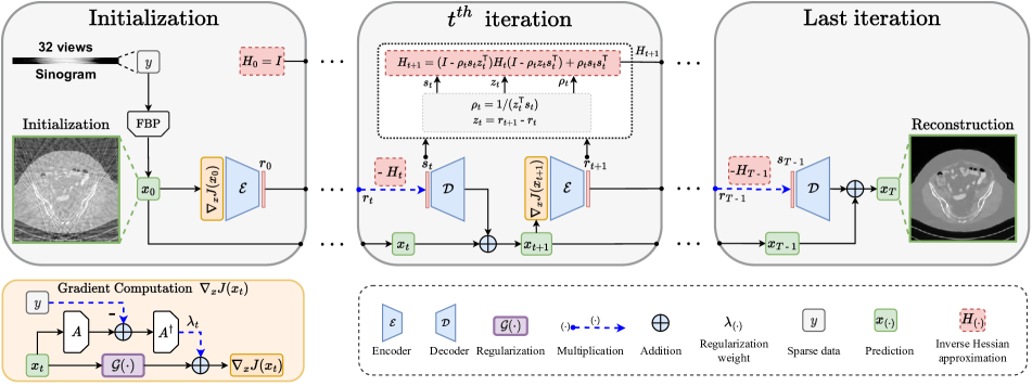
Figure 2: Overall structure of the proposed QN-Mixer for sparse-view CT reconstruction, unrolled from Algorithm 2. The method leverages the advantages of the quasi-Newton method for faster convergence while incorporating a latent BFGS update.

Recent advances in sparse-view CT reconstruction leverage two main categories of deep learning methods: post-processing and dual-domain approaches. Post-processing methods, including RedCNN [5], FBPConvNet [17], and DDNet [54], treat sparse-view reconstruction as a denoising step using FBP reconstructions as input. While effective in addressing artifacts and reducing noise, they often struggle with recovering global information from extremely sparse data. To overcome this limitation, dual-domain methods integrate sinograms into neural networks for an interpolation task, recovering missing data [22, 14]. Dual-domain methods, surpassing post-processing ones, combine information from both domains. DuDoNet [26], an initial dual-domain method, connects image and sinogram domains through a Radon inversion layer. Recent Transformer-based dual-domain methods, such as DuDoTrans [45] and DDPTransformer [24], aim to capture long-range dependencies in the sinogram domain, demonstrating superior performance to CNN-based methods.

2.3 Advancements in Deep Unrolling Networks

Unrolling networks constitute a line of work inspired by popular optimization algorithms used to solve Eq. 2. Leveraging the iterative nature of optimization algorithms, as presented in Eq. 4, unrolling networks aim to directly learn optimization parameters from data. These methods have found success in various inverse problems, including sparse-view CT [6, 18, 48, 52, 50], limited-angle CT [10, 47, 7], low-dose CT [1, 15], and compressed sensing MRI [41, 11].

First-order.  One pioneering unrolling network, Learned Primal-Dual reconstruction [1], replaces traditional proximal operators with CNNs. In contrast, LEARN [6] and LEARN++ [52] directly unroll the optimization algorithm from Eq. 4 into a deep recurrent neural network. More recently, Transformers [3, 28] have been introduced into unrolling networks, such as RegFormer [50] and HUMUS-Net [11]. While achieving commendable performance, these methods require more computational resources than traditional CNN-based unrolling networks and incur a significant memory footprint due to linear scaling with the number of unrolling iterations.

Second-order.  To address this, a new category of unrolling optimization methods has emerged [13], leveraging second-order techniques like the quasi-Newton method [19, 12, 9]. These methods converge faster, reducing computational demands, but struggle with increased memory usage due to Hessian matrix approximation and their application is limited to small-scale problems [27, 53]. In contrast our method propose a memory-efficient approach by operating within the latent space of gradient information (i.e. $\nabla_{\bm{x}}J({\bm{x}})$ in Eq. 3).

Data: ${\bm{y}}$ (sparse sinogram)

Manual choice of the regularization term ${\mathcal{R}}$;

${\bm{H}}_{0}\leftarrow{\bm{I}}^{n\times n}$;

${\bm{x}}_{0}\leftarrow{\bm{A}}^{\dagger}{\bm{y}}$;

for $t\in\{0,\dots,T-1\}$ do

       ${\bm{s}}_{t}\leftarrow-{\bm{H}}_{t}\nabla_{{\bm{x}}}J({\bm{x}}_{t})$

      ${\bm{x}}_{t+1}\leftarrow{\bm{x}}_{t}+{\bm{s}}_{t}$

      ${\bm{z}}_{t}\leftarrow\nabla_{{\bm{x}}}J({\bm{x}}_{t+1})-\nabla_{{\bm{x}}}J({\bm{x}}_{t})$

      $\rho_{t}\leftarrow 1/({\bm{z}}_{t}^{\mathsf{T}}{\bm{s}}_{t})$

      ${\bm{H}}_{t+1}\leftarrow({\bm{I}}-\rho_{t}{\bm{s}}_{t}{\bm{z}}_{t}^{\mathsf{T}}){\bm{H}}_{t}({\bm{I}}-\rho_{t}{\bm{z}}_{t}{\bm{s}}_{t}^{\mathsf{T}})+\rho_{t}{\bm{s}}_{t}{\bm{s}}_{t}^{\mathsf{T}}$

Algorithm 1 Quasi-Newton for sparse-view CT

3 Methodology

QN-Mixer is a novel second-order unrolling network inspired by the quasi-Newton (Sec. 3.1) method. It approximates the inverse Hessian matrix with a latent BFGS algorithm and includes a non-local regularization term, Incept-Mixer, designed to capture non-local relationships (Sec. 3.2). To cope with the significant computational burden associated with the full approximation of the inverse Hessian matrix, we use a latent BFGS algorithm (Sec. 3.3). An overview of the proposed method is depicted in Fig. 2, and the complete algorithm is presented in Sec. 3.4.

3.1 Quasi-Newton method

The quasi-Newton method can be applied to solve Eq. 2 and the iterative optimization solution is expressed as:

$${\bm{x}}_{t+1}={\bm{x}}_{t}-\alpha_{t}{\bm{H}}_{t}\nabla_{\bm{x}}J({\bm{x}}_{t}),$$ (5)

where ${\bm{H}}_{t}\in\mathbb{R}^{n\times n}$ represents the inverse Hessian matrix approximation at iteration $t$, and $\alpha_{t}$ is the step size. The BFGS method updates the Hessian matrix approximation in each iteration. This matrix is crucial for understanding the curvature of the objective function around the current point, guiding us to take more efficient steps and avoiding unnecessary zigzagging. In the classical BFGS approach, the line search adheres to Wolfe conditions [12, 9]. A step size of $\alpha_{t}=1$ is attempted first, ensuring eventual acceptance for superlinear convergence [19]. In our approach, we adopt a fixed step size of $\alpha_{t}=1$. The algorithm is illustrated in Algorithm 1.

3.2 Regularization term: Incept-Mixer

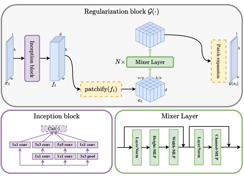
Figure 3: Architecture of our regularization block. It is referred to as “Incept-Mixer” and denoted as ${\mathcal{G}}$ in Eq. 4

Recent research on unrolling networks has often focused on selecting the representation of the regularization term gradient (i.e. ${\mathcal{G}}$ in Eq. 4), ranging from conv-nets [6, 52, 41] to more recent attention-based nets [50, 11]. In alignment with this trend, we introduce a non-local regularization block named Incept-Mixer and depicted in, Fig. 3. This block is crafted by drawing inspiration from both the multi-layer perceptron mixer [43] and the inception architecture [42], leveraging the strengths of each: capturing long-range interactions through the attention-like mechanism of MLP-Mixer and extracting local invariant features from the inception block. This design choice is evident in the ablation study (see Tab. 6) where Incept-Mixer outperforms both alternatives.

Starting from an image ${\bm{x}}_{t}\in\mathbb{R}^{h\times w\times c}$ at iteration $t$, we pass it through an Inception block to create a feature map ${\bm{f}}_{t}\in\mathbb{R}^{h\times w\times d}$, where $d$ is the depth of features. Subsequently, ${\bm{f}}_{t}$ undergoes patchification using a CNN with a kernel size and stride of $p$, representing the patch size. This process yields patch embeddings, ${\bm{e}}_{t}=\mathrm{patchify}({\bm{f}}_{t})\in\mathbb{R}^{\frac{h}{p}\times\frac{w}{p}\times d}$. These embeddings are then processed through a Mixer Layer with token and channel MLPs, layer normalization, and skip connections for inter-layer information flow, following [43]:

$$\begin{split}\mathrm{MixerLayer}({\bm{e}}_{t})&=\mathrm{Mix}(\mathrm{MLP}_{\texttt{channel}},\\ &\mathrm{Mix}(\left[\mathrm{MLP}_{\texttt{height}},\mathrm{MLP}_{\texttt{width}}\right],{\bm{e}}_{t}),\end{split}$$ (6)

where $\mathrm{Mix}(\mathrm{Layer},{\bm{e}}_{t})=\mathrm{Layer}(\mathrm{LN}({\bm{e}}_{t}))+{\bm{e}}_{t}$, with $\mathrm{LN}$ as layer normalization. $\mathrm{MLP}_{\texttt{height}}$, $\mathrm{MLP}_{\texttt{width}}$ are applied to height and width features, respectively, and $\mathrm{MLP}_{\texttt{channel}}$ to rows and shared. Finally, after $N$ such mixer layers, the regularized sample is transformed back to an image through a patch expansion step to obtain ${\mathcal{G}}({\bm{x}}_{t})$. Consequently, the iterative optimization solution is as follows:

$$\begin{aligned} &{\bm{x}}_{t+1}={\bm{x}}_{t}-{\bm{H}}_{t}\nabla_{\bm{x}}J({\bm{x}}_{t}),\\ &\text{where}\quad\nabla_{\bm{x}}J({\bm{x}}_{t})=\lambda_{t}{\bm{A}}^{\dagger}\left({\bm{A}}{\bm{x}}_{t}-{\bm{y}}\right)+{\mathcal{G}}({\bm{x}}_{t}).\end{aligned}$$ (7)

Here, ${\mathcal{G}}({\bm{x}}_{t})$ denotes the Incept-Mixer model, representing the learned gradient of the regularization term.

3.3 Latent BFGS update

We propose a memory-efficient latent BFGS update. Drawing inspiration from LDMs [38], At step $t$, given the gradient value $\nabla_{{\bm{x}}}J({\bm{x}}_{t})\in\mathbb{R}^{h\times w\times c}$, the encoder $\mathcal{E}$ encodes it into a latent representation ${\bm{r}}_{t}=\mathcal{E}(\nabla_{{\bm{x}}}J({\bm{x}}_{t}))\in\mathbb{R}^{l_{h}\cdot l_{w}}$. Importantly, the encoder downsamples the gradient by a factor ${\bm{f}}_{\mathcal{E}}=\frac{h}{h_{l}}=\frac{w}{w_{l}}$. Throughout the paper, we explore different downsampling factors (see Tab. 5) ${\bm{f}}_{\mathcal{E}}=2^{k}$, where $k\in{\mathbb{N}}$ is the number of downsampling stacks. Encoding the gradient reduces the optimization variable size of BFGS (i.e. ${\bm{H}}_{t}\in\mathbb{R}^{(l_{h}\cdot l_{w})\times(l_{h}\cdot l_{w})}$), thereby decreasing the computational cost associated with high memory demand. The direction is then computed in the latent space $s_{t}=-{\bm{H}}_{t}{\bm{r}}_{t}$, and finally, the decoder $\mathcal{D}$ reconstructs the update from the latent direction, giving $\mathcal{D}(s_{t})=\mathcal{D}(-{\bm{H}}_{t}\mathcal{E}(\nabla_{{\bm{x}}}J({\bm{x}}_{t})))\in\mathbb{R}^{h\times w\times c}$. It is noteworthy that $\mathcal{E}$ and $\mathcal{D}$ are shared across the algorithm iterations, as shown in Fig. 2.

3.4 Proposed algorithm of QN-Mixer

Data: ${\bm{y}}$ (sparse sinogram)

${\bm{H}}_{0}\leftarrow{\bm{I}}^{(l_{h}\cdot l_{w})\times(l_{h}\cdot l_{w})}$;

${\bm{x}}_{0}\leftarrow{\bm{A}}^{\dagger}{\bm{y}}$;

${\bm{r}}_{0}\leftarrow\mathcal{E}(\nabla_{{\bm{x}}}J({\bm{x}}_{0}))$;

for $t\in\{0,\dots,T-1\}$ do

       ${\bm{s}}_{t}\leftarrow-{\bm{H}}_{t}{\bm{r}}_{t}$

      ${\bm{x}}_{t+1}\leftarrow{\bm{x}}_{t}+\mathcal{D}({\bm{s}}_{t})$

      ${\bm{r}}_{t+1}\leftarrow\mathcal{E}(\nabla_{{\bm{x}}}J({\bm{x}}_{t+1}))$

      ${\bm{z}}_{t}\leftarrow{\bm{r}}_{t+1}-{\bm{r}}_{t}$

      $\rho_{t}\leftarrow 1/({\bm{z}}_{t}^{\mathsf{T}}{\bm{s}}_{t})$

      ${\bm{H}}_{t+1}\leftarrow({\bm{I}}-\rho_{t}{\bm{s}}_{t}{\bm{z}}_{t}^{\mathsf{T}}){\bm{H}}_{t}({\bm{I}}-\rho_{t}{\bm{z}}_{t}{\bm{s}}_{t}^{\mathsf{T}})+\rho_{t}{\bm{s}}_{t}{\bm{s}}_{t}^{\mathsf{T}}$

Algorithm 2 QN-Mixer (latent BFGS update)

Our method, builds on the BFGS update [12, 9] rank-one approximation for the inverse Hessian. This approximation serves as a preconditioning matrix, guiding the descent direction. In contrast to [13], which directly learns the inverse Hessian approximation from data, our approach incorporates the mathematical equations of the BFGS algorithm for more accurate approximations. The full QN-Mixer algorithm is illustrated in Algorithm 2.

Method	No noise $(N_{0}=0)$						Low noise $(N_{1}=10^{6})$						High noise $(N_{2}=5\times 10^{5})$
	$n_{v}=32$		$n_{v}=64$		$n_{v}=128$		$n_{v}=32$		$n_{v}=64$		$n_{v}=128$		$n_{v}=32$		$n_{v}=64$		$n_{v}=128$
	PSNR $\uparrow$	SSIM $\uparrow$	PSNR $\uparrow$	SSIM $\uparrow$	PSNR $\uparrow$	SSIM $\uparrow$	PSNR $\uparrow$	SSIM $\uparrow$	PSNR $\uparrow$	SSIM $\uparrow$	PSNR $\uparrow$	SSIM $\uparrow$	PSNR $\uparrow$	SSIM $\uparrow$	PSNR $\uparrow$	SSIM $\uparrow$	PSNR $\uparrow$	SSIM $\uparrow$
FBP	22.65	40.49	27.29	57.94	33.04	79.50	22.09	32.73	26.51	49.56	31.69	71.09	19.05	15.56	22.71	25.74	26.52	40.87
FBPConvNet [17]	30.32	85.11	35.42	90.15	39.71	94.64	30.20	84.46	35.09	89.72	39.06	94.08	29.91	82.52	34.13	87.85	36.89	91.28
DuDoTrans [45]	30.48	84.70	35.37	91.87	40.62	96.41	30.34	83.72	35.36	91.42	39.75	95.49	30.09	81.83	34.09	88.67	37.08	93.44
Learned PD [1]	35.88	92.09	41.03	96.28	43.33	97.31	35.78	92.21	39.03	94.79	41.65	96.44	33.80	89.23	37.34	93.23	39.17	94.69
LEARN [6]	37.58	94.65	42.26	97.25	43.11	97.57	36.95	93.63	39.91	95.82	42.17	97.11	34.38	90.51	37.15	93.53	39.38	95.18
RegFormer [50]	38.71	95.42	43.56	97.76	47.95	98.98	37.21	94.73	41.65	96.92	44.38	98.02	35.93	92.78	38.53	94.84	40.52	96.19
QN-Mixer (ours)	39.51	96.11	45.57	98.48	50.09	99.32	37.50	94.92	42.46	97.70	44.27	98.11	35.91	92.49	38.73	94.92	40.51	96.27

Table 1: Quantitative evaluation on AAPM of state-of-the-art methods (PSNR in dB and SSIM in %). Bold: Best, under: second best.

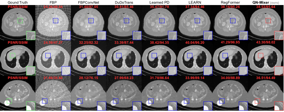
Figure 4: Visual comparison on AAPM. From top to bottom: the results under the following conditions: first $(n_{v}=32,N_{1})$, second $(n_{v}=64,N_{1})$, third $(n_{v}=32,N_{0})$. The last row presents out-of-distribution (OOD) results with a randomly overlaid circle on a test image. The display window is set to $\left[-1000,800\right]$ HU.

4 Experiments

In this section, we initially present our experimental settings, followed by a comparison of our approach with other state-of-the-art CT reconstruction methods. Finally, we delve into the contribution analysis of each component in our model.

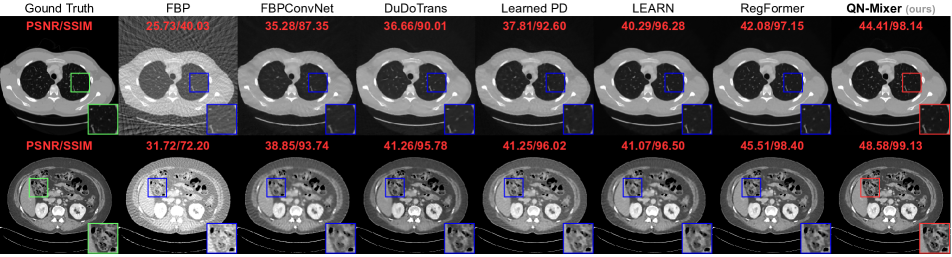
Figure 5: Visual comparison on DeepLesion of state-of-the-art methods. Rows display results under different conditions: $(n_{v}=64,N_{1})$ and $(n_{v}=128,N_{1})$. Display windows are set to $\left[-1000,800\right]$ HU for the first row and $\left[-200,300\right]$ HU for the second row.

4.1 Experimental Setup

Datasets.  We evaluate our method on two widely used datasets: the “2016 NIH-AAPM-Mayo Clinic Low-Dose CT Grand Challenge” dataset (AAPM) [32] and the DeepLesion dataset [51]. The AAPM dataset comprises 2378 full-dose CT images from 10 patients, while DeepLesion is the largest publicly accessible multi-lesion real-world CT dataset, including 4427 unique patients.

Implementation details.  For AAPM, we select $1920$ training images from 8 patients, $244$ validation images from $1$ patient, and $214$ testing images from the last patient. For DeepLesion, we select a subset of $2000$ training images and $300$ testing images randomly from the official splits. All images are resized to $256\times 256$ pixels. To simulate the forward and backprojection operators, we use the Operator Discretization Library (ODL) [36] with a 2D fan-beam geometry ($512$ detector pixels, source-to-axis distance of $600$ mm, axis-to-detector distance of $290$ mm). Sparse-view CT images are generated with $n_{v}\in\{32,64,128\}$ projection views, uniformly sampled from a full set of $512$ views covering $\left[0,2\pi\right]$. To mimic real-world CT images, we introduce mixed noise to the sinograms, combining 5% Gaussian noise and Poisson noise with an intensity of $1\times 10^{6}$.

Training details.  For each set of $n_{v}$ views, we train our model for $50$ epochs using $4$ Nvidia Tesla V100 (32GB RAM). We employ the AdamW optimizer [29] with a learning rate of $1\times 10^{-4}$, weight decay $1\times 10^{-2}$, and utilize the mean squared error loss with a batch size of $1$. Additionally, we incorporate a learning rate decay factor of $0.1$ after $40$ epochs. Unrolling iterations for QN-Mixer are set to $T=14$. Incept-Mixer uses a patch size of $p=4$, $d=96$ embedding dimension, and $N=2$ mixer layers. The inverse Hessian size is $64^{2}\times 64^{2}$ with $k=2$ downsampling blocks. Following [50], ${\bm{A}}^{\dagger}$ is implemented using the FBP algorithm for the pseudo-inverse of ${\bm{A}}$.

Evaluation metrics.  Consistent with standard evaluation practices [1, 45, 50], we use the structural similarity index measure (SSIM) with parameters set to: level${~{}\text{=}~{}}5$, a Gaussian kernel of size $11$, and a standard deviation of $1.5$ as our primary performance indicator. Additionally, we complement our evaluation with the peak signal-to-noise ratio (PSNR).

State-of-the-art baselines.  We compare QN-Mixer to multiple state-of-the-art competitors: (1) post-processing based denoising methods, i.e., FBPConvNet [17], and DuDoTrans [45]; (2) first-order unrolling reconstruction networks, i.e., Learned Primal-Dual [1], LEARN [6], and RegFormer [50]. Note that we replace the pseudo-inverse operator used by LEARN with the FBP algorithm, as it has been demonstrated to be more effective according to [50]. To ensure a fair comparison, we utilize the code-base released by the authors when possible or meticulously implement the methods based on the details provided in their papers. All approaches undergo training and testing on the same datasets, as elaborated in implementation details.

4.2 Comparison with state-of-the-art methods

Method	$n_{v}=32$		$n_{v}=64$		$n_{v}=128$
	PSNR $\uparrow$	SSIM $\uparrow$	PSNR $\uparrow$	SSIM $\uparrow$	PSNR $\uparrow$	SSIM $\uparrow$
FBP	21.55	31.65	26.07	47.17	31.49	69.63
FBPConvNet [17]	30.74	80.41	34.64	87.36	38.69	92.94
DuDoTrans [45]	32.11	79.86	36.02	88.14	40.47	93.81
Learned PD [1]	34.02	88.44	37.56	92.46	40.79	95.32
LEARN [6]	35.76	92.12	39.83	95.66	41.34	96.21
RegFormer [50]	37.38	93.89	41.70	96.78	46.10	98.39
QN-Mixer (ours)	39.39	95.67	43.75	97.73	48.62	98.64

Table 2: Quantitative evaluation on DeepLesion for state-of-the-art methods (PSNR in dB and SSIM in %). With Poisson noise level of $N_{1}=10^{6}$. Bold: Best, under: second best.

Quantitative comparison.  We compared our model with state-of-the-art baselines on two public datasets. For AAPM, models were trained and tested across three projection views ($n_{v}\in\{32,64,128\}$) and three noise levels, namely no noise $N_{0}=0$, low noise $N_{1}=10^{6}$, and high noise $N_{2}=5\times 10^{5}$ (see Tab. 1). For DeepLesion, models were trained and tested on the same three projection views and a noise level of $N_{1}=10^{6}$ (see Tab. 2). Visual results are provided in Fig. 4 (AAPM) and Fig. 5 (DeepLesion). Impressively, our method achieves state-of-the-art results on DeepLesion across all projection views. It outperforms the second-best baseline, RegFormer, with an average improvements of $+2.23$ dB in PSNR and $+1.02$% in SSIM. On AAPM without noise, we achieve state-of-the-art results across all projection views and improve the second best by an average $+1.65$ dB and $+0.58\%$. In the presence of low noise, QN-Mixer achieves state-of-the-art results performance in all cases except $n_{v}=128$ with $-0.11$ dB and shows an average improvements of $+0.33$ dB and $+0.35$% over RegFormer. With high noise, our method performs nearly on par in $n_{v}=32$ ($-0.02$ dB and $-0.29$%), achieves state-of-the-art in $n_{v}=64$ ($+0.2$ dB and $+0.08$%), and competes closely in $n_{v}=128$ ($-0.01$ dB and $+0.08$%). As noise increases, we attribute the decline in improvement to the compressed gradient information in the latent BFGS, influenced by sinogram changes, and the utilization of the FBP algorithm instead of the pseudo-inverse.

Performance comparison on OOD textures.

Method	$n_{v}=32$		$n_{v}=64$		$n_{v}=128$
	PSNR $\uparrow$	SSIM $\uparrow$	PSNR $\uparrow$	SSIM $\uparrow$	PSNR $\uparrow$	SSIM $\uparrow$
FBP	21.38	33.36	26.08	50.29	31.43	73.06
FBPConvNet [17]	28.05	75.96	32.50	82.90	35.45	88.14
DuDoTrans [45]	28.11	68.17	32.71	83.26	36.41	90.36
Learned PD [1]	31.96	87.10	36.40	92.57	37.63	93.17
LEARN [6]	34.48	90.15	36.89	91.85	38.32	94.67
RegFormer [50]	34.49	89.98	36.95	91.48	38.02	92.44
QN-Mixer (ours)	36.84	94.84	42.11	97.78	45.69	98.82

Table 3: Quantitative evaluation on out-of-distribution (OOD) AAPM test dataset of state-of-the-art methods (PSNR in dB and SSIM in %). Bold: Best, under: second best.

In medical imaging, where training data predominantly consists of normal patient images, it is imperative to develop methods that generalize to scans with lesions or anomalies. To address this challenge, we conducted an experiment to evaluate model performance on out-of-distribution (OOD) textures. The frozen models were tested with CT images featuring a randomly positioned white circle with no noise added to the sinograms, as illustrated in the third row of Fig. 4. In Tab. 3, QN-Mixer attains state-of-the-art results across all $n_{v}$ views. First-order unrolling networks such as LEARN and RegFormer exhibit significant PSNR degradation of $-3.1$ dB and $-4.22$ dB, respectively, for $n_{v}=32$, while our method demonstrates a milder degradation of $-2.67$ dB.

Visual comparison.  As it can be seen on Fig. 4 and Fig. 5, FBPConvNet and DuDoTrans exhibit noticeable blurry images with severe artifacts when $n_{v}=32$. While Learned PD and LEARN show satisfactory performance, they struggle with intricate details, like in the liver and spine. In contrast, RegFormer produces high-quality images but faces challenges in generalizing to OOD data. QN-Mixer excels in producing high-quality images with fine details, even under challenging conditions such as $n_{v}=32$ views and OOD data.

Method	#Iters	Epoch time (s)	#Params (M)	Memory (GB)
FBPConvNet [17]	-	68	31.1	1.30
DuDoTrans [45]	-	92	15.0	1.38
Learned PD [1]	10	82	0.25	0.81
LEARN [6]	30	780	4.50	1.85
RegFormer [50]	18	700	5.00	10.19
QN-Mixer (ours)	14	594	8.50	7.83

Table 4: Comparison of computational efficiency. Training epoch time is reported in seconds, #Params in M and memory costs for state-of-the-art methods on AAPM with $n_{v}=32$ views.

Efficiency comparison.  The results in Tab. 4 show that QN-Mixer is more computationally efficient than RegFormer, with a $1.3\times$ reduction in memory usage. Furthermore, our training time demonstrates a significant enhancement, realizing a speed improvement of $106$ seconds per epoch compared to first-order unrolling methods like LEARN and RegFormer. Additionally, our method requires only $14$ iterations, in contrast to the $30$ and $18$ iterations needed by LEARN and RegFormer, respectively.

Hessian size	PSNR $\uparrow$	SSIM $\uparrow$
$8^{2}\times 8^{2}$	35.69	93.71
$16^{2}\times 16^{2}$	38.11	95.31
$32^{2}\times 32^{2}$	39.37	96.01
[2pt/4pt] $64^{2}\times 64^{2}$	39.51	96.11

Table 5: Ablation on the inverse Hessian approximation size.

Method	PSNR $\uparrow$	SSIM $\uparrow$
QN+Inception	31.65	85.28
QN+MLP-Mixer	36.89	93.87
[2pt/4pt] QN-Mixer+${\bm{A}}^{\dagger}$	38.94	95.83
[2pt/4pt] Incept-Mixer + first-order	37.45	94.25
QN-Mixer (ours)	39.51	96.11

Table 6: Ablation for the regularization term. ${\bm{A}}^{\dagger}$ denotes the pseudo-inverse.

4.3 Ablation Study

In this section, we leverage the AAPM dataset with $n_{v}=32$ views by default, and no noise is introduced to the sinogram.

Inverse Hessian approximation size.  The results in Tab. 5 emphasize the significant impact of the inverse Hessian approximation size on our performance. When too small, a notable degradation is observed (e.g., $8^{2}\times 8^{2}$), while larger sizes result in performance improvements as the approximation approaches the full inverse Hessian. However, exceeding $64^{2}\times 64^{2}$ was unfeasible in our experiments due to increasing memory costs and memory constraints.

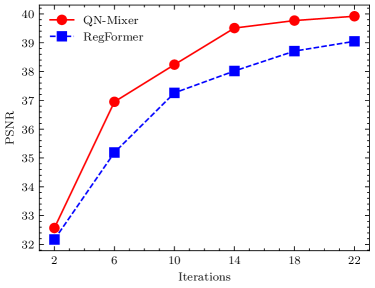
(a)

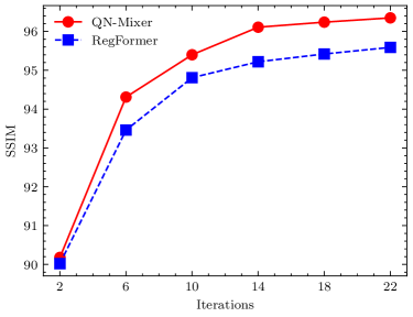
(b)

Figure 6: Ablation on the number of unrolling iterations. We compare our QN-Mixer against RegFormer. Left: PSNR (dB); Right: SSIM (%)

Number of unrolling iterations.  In Fig. 6, we visually depict the influence of the number of unrolling iterations on the performance of QN-Mixer and RegFormer. Notably, the performance of both methods shows improvement with an increase in the number of iterations. When subjected to an equal number of iterations, our method consistently surpasses RegFormer in performance. Remarkably, we achieve comparable results to RegFormer even with only 10 iterations, demonstrating the efficiency of our approach.

Regularization term.  We evaluate the impact of the regularization term in our framework. Our Incept-Mixer is compared against various learned alternatives, including the Inception block [42] and MLP-Mixer block [43]. Additionally, we explore the use of the pseudo-inverse ${\bm{A}}^{\dagger}$ instead of the FBP. The results presented in Tab. 6 show that employing the pseudo-inverse results in a less pronounced degradation ($-0.57$ dB and $-0.28$%), enhancing the interpretability of QN-Mixer. Finally, we test our Incept-Mixer in the first-order framework, highlighting the significance of the second-order latent BFGS approximation with a significant improvement ($+2.06$ dB and $+1.86\%$).

5 Conclusion

In this paper, we investigate the application of deep second-order unrolling networks for tackling imaging inverse problems. To this end, we introduce QN-Mixer, a quasi-Newton inspired algorithm where a latent BFGS method approximates the inverse Hessian, and our Incept-Mixer serves as the non-local learnable regularization term. Extensive experiments confirm the successful sparse-view CT reconstruction by our model, showcasing superior performance with fewer iterations than state-of-the-art methods. In summary, this research offers a fresh perspective that can be applied to any iterative reconstruction algorithm. A limitation of our work is the memory requirements associated with quasi-Newton algorithm. We introduced a memory-efficient alternative by projecting the gradient to a lower dimension, successfully addressing the CT reconstruction problem. However, its applicability to other inverse problems may be limited. In future work, we aim to extend our approach to handle larger Hessian sizes, broadening its application to a range of problems.

Supplementary Material

1

 

1 Inverse Hessian approximation

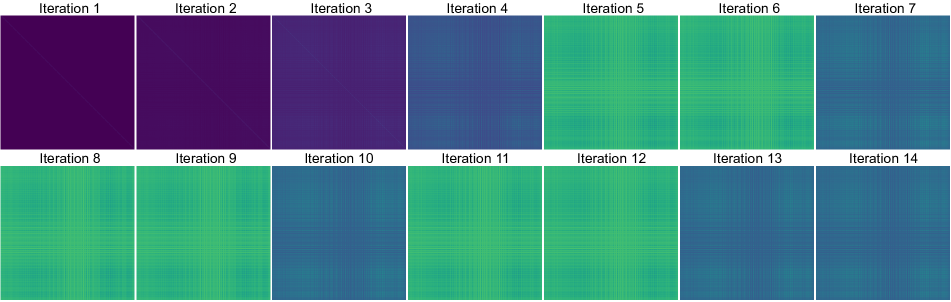
Figure 7: Visualization of the inverse Hessian approximation across iterations. Observe the subtle changes between each iteration, attributed to the influence of the objective function used to estimate $H_{t}$ (see Eq. 10).

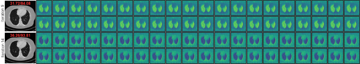
Figure 8: Inverse Hessian approximation rows visualization. We present the first $40$ rows for the $9^{th}$ and $14^{th}$ inverse Hessian approximations on the first and second lines, respectively. Each row is of size $64^{2}$, reshaped into a $64\times 64$ image. The corresponding image reconstructions are shown on the left, along with PSNR (dB) and SSIM (%) values at the top.

1.1 Approximation via optimization

The fundamental idea is to iteratively build a recursive approximation by utilizing curvature information along the trajectory. It is crucial to emphasize that a quadratic approximation offers a direction that can be leveraged within the iterative update scheme. This direction is defined by the equation:

$${\bm{x}}_{t+1}={\bm{x}}_{t}+\alpha_{t}{\bm{d}}_{t}.$$ (8)

In order to determine the direction ${\bm{d}}_{t}$, we can employ a quadratic approximation of the objective function. This approximation can be expressed as:

$$J({\bm{x}}_{t}+{\bm{d}})\approx m_{t}({\bm{d}})=J({\bm{x}}_{t})+\nabla J({\bm{x}}_{t})^{\mathsf{T}}{\bm{d}}+\frac{1}{2}{\bm{d}}^{\mathsf{T}}{\bm{B}}_{t}{\bm{d}},$$ (9)

where $J({\bm{x}}_{t})$ represents the objective function evaluated at the current point ${\bm{x}}_{t}$, $\nabla J({\bm{x}}_{t})$ denotes the gradient of the objective function at ${\bm{x}}_{t}$, ${\bm{B}}_{t}\in\mathbb{R}^{n\times n}$ corresponds to the approximation of the Hessian matrix. By minimizing the right-hand side of the quadratic approximation in Eq. 9, we can determine the optimal direction ${\bm{d}}_{t}$. Taking the derivative of $m_{t}({\bm{d}})$ with respect to ${\bm{d}}$ and setting it to zero, we obtain:

$$\frac{\nabla m_{t}({\bm{d}})}{\nabla{\bm{d}}}={\bm{d}}_{t}{\bm{B}}_{t}+\nabla J({\bm{x}}_{t})\xrightarrow{\nabla m_{t}({\bm{d}})=0}{\bm{d}}_{t}=-{\bm{B}}_{t}^{-1}\nabla J({\bm{x}}_{t}),$$

by substituting this result in Eq. 8 we obtain:

$${\bm{x}}_{t+1}={\bm{x}}_{t}-\alpha_{t}{\bm{B}}_{t}^{-1}\nabla J({\bm{x}}_{t}).$$

The objective is to ensure that the curvature along the trajectory is consistent. In other words, at the last two iterations, $m_{t+1}$ should match the gradient $\nabla J({\bm{x}}_{t})$ in the following way:

$$\nabla m_{t+1}\bigg{|}_{{\bm{d}}=0}=\nabla J({\bm{x}}_{t+1}),\ \nabla m_{t+1}\bigg{|}_{{\bm{d}}=-\alpha_{t}{\bm{d}}_{t}}=\nabla J({\bm{x}}_{t}).$$

This condition ensures that the quadratic approximation captures the correct curvature information along the trajectory, allowing for accurate optimization and convergence of the algorithm. By evaluating $\nabla m_{t+1}(\cdot)$ at the point $-\alpha_{t}{\bm{d}}_{t}$ we obtain:

$$\alpha_{t}{\bm{B}}_{t+1}{\bm{d}}_{t}=\nabla J({\bm{x}}_{t+1})-\nabla J({\bm{x}}_{t}).$$

From Eq. 8 we get the secant equation:

$${\bm{B}}_{t+1}{\color[rgb]{0.171875,0.62890625,0.171875}\underbrace{\text{$({\bm{x}}_{t+1}-{\bm{x}}_{t})$}}_{\text{${\bm{s}}_{t}$}}}={\color[rgb]{0,0.265625,0.66796875}\underbrace{\text{$\nabla J({\bm{x}}_{t+1})-\nabla J({\bm{x}}_{t})$}}_{\text{${\bm{z}}_{t}$}}}\rightarrow{\bm{B}}_{t+1}{\color[rgb]{0.171875,0.62890625,0.171875}\text{${\bm{s}}_{t}$}}={\color[rgb]{0,0.265625,0.66796875}\text{${\bm{z}}_{t}$}}.$$

To avoid explicitly computing the inverse matrix ${\bm{B}}_{t}^{-1}$, we can introduce an approximation ${\bm{H}}_{t}={\bm{B}}_{t}^{-1}$ and optimize it as follows:

$${\bm{H}}_{t+1}=\underset{{\bm{H}}}{\operatorname{arg}\,\operatorname{min}} \left\lVert{\bm{H}}-{\bm{H}}_{t}\right\rVert^{2}_{\bm{W}} \rhd{\bm{H}}_{t+1}\ \text{close to}\ {\bm{H}}_{t}$$ (10)

s.t.: $${\bm{H}}={\bm{H}}^{\mathsf{T}} \rhd\ \text{symmetry}$$

$${\bm{H}}{\bm{z}}_{t}={\bm{s}}_{t} \rhd\text{secant equation}$$

Here $\left\lVert\cdot\right\rVert_{\bm{W}}^{2}$ denotes the weighted Frobenius norm. This optimization problem aims to find an updated approximation ${\bm{H}}_{t+1}$ that is close to ${\bm{H}}_{t}$, while satisfying the constraints that ${\bm{H}}_{t+1}$ is symmetric and satisfies the secant equation ${\bm{H}}_{t+1}{\bm{z}}_{t}={\bm{s}}_{t}$. BFGS [12, 9, 19] uses ${\bm{W}}=\int_{0}^{1}\nabla^{2}J({\bm{x}}_{t}+t\alpha_{t}{\bm{d}}_{t})dt$, to solve this optimization problem and obtain the iterative update of ${\bm{H}}$:

$${\bm{H}}_{t+1}=({\bm{I}}-\rho_{t}{\bm{s}}_{t}{\bm{z}}_{t}^{\mathsf{T}}){\bm{H}}_{t}({\bm{I}}-\rho_{t}{\bm{z}}_{t}{\bm{s}}_{t}^{\mathsf{T}})+\rho_{t}{\bm{s}}_{t}{\bm{s}}_{t}^{\mathsf{T}},$$ (11)

where $\rho_{t}=\frac{1}{{\bm{z}}_{t}^{\mathsf{T}}{\bm{s}}_{t}}$, ${\bm{s}}_{t}={\bm{x}}_{t+1}-{\bm{x}}_{t}$, and ${\bm{z}}_{t}=\nabla J({\bm{x}}_{t+1})-\nabla J({\bm{x}}_{t})$. This update equation allows us to iteratively refine the approximation ${\bm{H}}_{t}$ based on the current gradient information and the changes in the solution.

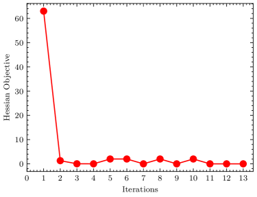
(a)

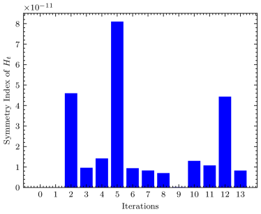
(b)

Figure 9: Inverse Hessian matrix approximation algorithm. Verification of requirements over the iterations. Left: Objective function value in Eq. 10; Right: Symmetry index of the inverse Hessian approximation refer to Eq. 12.

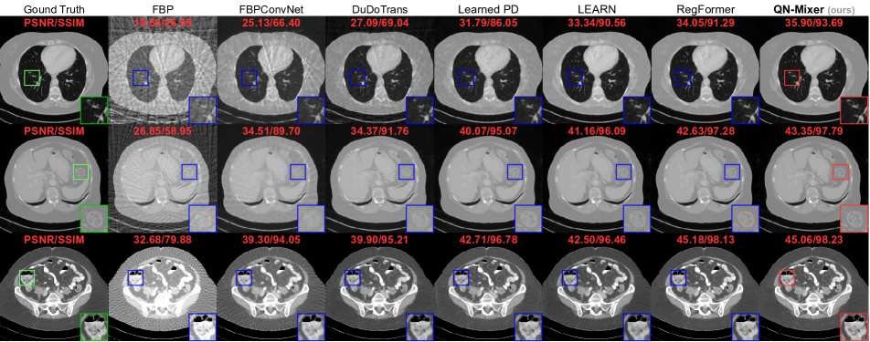
Figure 10: Visual comparison on AAPM. From top to bottom: the results under the following conditions: first $(n_{v}=32,N_{1})$, second $(n_{v}=64,N_{1})$, third $(n_{v}=128,N_{1})$. The display window is set to $\left[-1000,800\right]$ HU for the first two rows and to $\left[-200,300\right]$ HU for the last row.

1.2 Validation of adherence to BFGS

We validate the adherence of our method to the BFGS requirements. To achieve this, we present the constraint values of the optimization algorithm given in Eq. 10 using a test set image from AAPM, as illustrated in Fig. 9. The symmetry index is defined as follows:

$$SI=\frac{1}{{n\cdot(n-1)}}\sum_{i=1}^{n}\sum_{j=1,j\neq i}^{n}\lvert{\bm{A}}_{ij}-{\bm{A}}_{ji}\rvert.$$ (12)

Our results demonstrate the effectiveness of our approach in satisfying the essential conditions required by the BFGS algorithm. Notably, the symmetry index is consistently close to zero, indicating the symmetry of the matrix ${\bm{H}}_{t}$ at each iteration, which is the first constraint of the BFGS method. Furthermore, with regard to the objective function value, it is evident that it is close to zero, except for the initial approximation. This deviation can be attributed to the use of the identity matrix as the starting point.

Inverse Hessian matrix approximation visualizations.

Figure 7 depicts ${\bm{H}}_{t}$ at different iterations. These visualizations confirm the required symmetry of the matrix in each iteration. Additionally, the matrix ${\bm{H}}_{t}$ is close to the identity matrix at the second iteration, becoming more structured in the third iteration. This behavior aligns with expectations, as the matrix ${\bm{H}}_{t}$ is initialized as the identity matrix and updated based on gradient information and solution changes.

Visualization of reshaped rows.

To further understand the inverse Hessian matrix approximation structure, we depict the reshaped ($64\times 64$) first $40$ rows of ${\bm{H}}_{t}$ at iterations $9$ and $14$ in Fig. 8. These rows store gradient attention information used for updating the solution, consistent with the matrix ${\bm{H}}_{t}$ being updated based on gradient information and solution changes. In future work, we plan to explore the impact of ${\bm{H}}_{t}$ on the optimization process and its influence on reconstruction performance.

2 More Ablation Study and Analysis

2.1 Ablation on Incept-Mixer

We further investigate the impact of the hyperparameters of Incept-Mixer on the reconstruction performance. We vary the patch size $p$ and the number of stacked Mixer layers $N$ and report the results in Tab. 7(a), and Tab. 7(b) respectively.

Impact of the path size.

We observe that increasing the patch size $p$ from $2$ to $4$ improves the performance ($+1.28$ dB and $+1.04$%) while further increasing the patch size from $4$ to $8$ decreases the performance ($-1.32$ dB and $-0.79$%).

We attribute this observed pattern to the trade-off between local and global features in the reconstruction process. When the patch size is small, such as $p=2$, the model focuses on capturing fine-grained local details, which can enhance reconstruction accuracy. As the patch size increases to $p=4$, the network gains a broader perspective by considering larger regions, leading to an improvement in performance. However, when the patch size becomes too large, for example, $p=8$, the model might start incorporating more global context at the expense of losing finer details. This can result in a decrease in performance as the model becomes less sensitive to localized patterns.

$p$	PSNR $\uparrow$	SSIM $\uparrow$
2	38.22	95.07
4	39.51	96.11
8	38.19	95.32

(a)

$N$	PSNR $\uparrow$	SSIM $\uparrow$
1	37.64	94.79
2	39.51	96.11
3	38.47	95.51
4	38.17	95.40

(b)

Table 7: Ablation of Incept-Mixer. (a) $p$ is the patch size; (b) $N$ is the number of stacked Mixer layers. The best performance is attained using $p=4$ and $N=2$.

Impact of the number of stacked Mixer layer.

We observe that increasing the number of stack $N$ from $1$ to $2$ improves the performance ($+1.86$ dB and $+1.31$%), while further increasing the patch size from $2$ to $3$ decreases the performance ($-1.03$ dB and $-0.60$%) and from $3$ to $4$ decreases the performance ($-0.30$ dB and $-0.11$%).

Similarly, when varying the number of stacked Mixer layers $N$, we observe a trend where an increase in $N$ initially contributes to improved performance, as the model can capture more complex features and relationships. However, as $N$ continues to grow, the network may encounter diminishing returns, and the benefits of additional layers diminish, potentially leading to overfitting or increased computational overhead.

Robustness to hyperparameters.

Hence, there exists an optimal trade-off between the patch size $p$ and the number of stacked Mixer layers $N$, but the model performs similarly for a wide range of values. In our experiments, we use $p=4$ and $N=2$ for all the datasets, which highlights the robustness of our method to these hyperparameters.

2.2 More visualization results

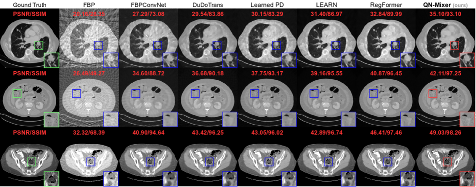
Figure 11: Visual comparison on DeepLesion. From top to bottom: the results under the following conditions: first $(n_{v}=32,N_{1})$, second $(n_{v}=64,N_{1})$, third $(n_{v}=128,N_{1})$. The display window is set to $\left[-1000,800\right]$ HU for the first two rows and to $\left[-200,300\right]$ HU for the last row.

Fig. 10 displays supplementary visualizations of our approach on AAPM. Our method consistently produces high-quality reconstructions across all views. Notably, among state-of-the-art techniques, QN-Mixer excels in reconstructing fine-grained details. For instance, it accurately captures small vessels in the first row, delicate soft tissue structures in the second row, and sharp boundaries in the third row.

In Fig. 11, we showcase additional visualizations of our method applied to DeepLesion. QN-Mixer demonstrates superior performance across all views, yielding high-quality reconstructions. This is particularly evident in the challenging scenario of $32$ views, where our method outperforms others in capturing fine-grained details, such as small vessels and lesions. Importantly, these results are achieved with fewer iterations compared to alternative unrolling networks like RegFormer.

2.3 Iterative results visualization

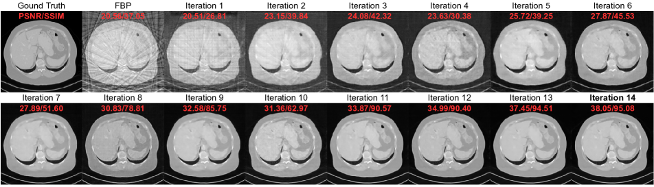
Figure 12: QN-Mixer’s intermediate reconstructions using AAPM with $(n_{v}=32,N_{1})$. Display window is set to $\left[-1000,800\right]$ HU.

In order to demonstrate the effectiveness of QN-Mixer, we present a series of intermediate reconstruction results in Fig. 12. These results illustrate the progression of the reconstruction process at different iterations of our method. By examining the reconstructed outputs at each iteration, our goal is to offer insights into the evolution of image quality. Notably, we observe that the improvement in quality, as quantified by the PSNR and SSIM values of each iteration, does not consistently increase with each iteration (see Iteration $10$ in Fig. 12). We suspect that the observed unexpected behavior may arise from the variation of the objective function (i.e. Eq. 2) around the point $t$ in the unrolled network, which is dependent on a learnable gradient regularization term Incept-Mixer.

2.4 More OOD results and visualization

Method	$n_{v}=32$		$n_{v}=64$		$n_{v}=128$
	SSIM $\uparrow$	PSNR $\uparrow$	SSIM $\uparrow$	PSNR $\uparrow$	SSIM $\uparrow$	PSNR $\uparrow$
FBP	72.88	18.97	83.42	22.13	91.75	24.85
FBPConvNet [17]	63.91	20.94	73.02	24.12	80.60	25.74
DuDoTrans [45]	60.51	19.09	79.75	25.00	85.65	27.23
Learned PD [1]	67.99	21.92	83.79	25.51	85.42	25.86
LEARN [6]	79.70	24.46	84.44	26.74	88.16	26.20
RegFormer [50]	72.45	23.69	77.33	25.46	84.99	28.22
QN-Mixer (ours)	86.17	25.95	94.56	30.95	97.04	33.98

Table 8: Quantitative results of the reconstruction of the cropped OOD circle. Bold: Best, under: second best.

In our initial analysis, we assess the robustness of methods to out-of-distribution (OOD) data using complete patient images, computing SSIM and PSNR metrics for the entire image. While achieving the best performance across all views, we observe a degradation in performance for all methods when focusing on the circle region, as expected due to its complexity.

To address this, we extend our evaluation to specific regions, those containing the white circles. This targeted approach isolates the reconstruction performance exclusively to the circle region. Our experiments involve a randomly selected $5$ samples from the AAPM test set depicted in Fig. 13. The overall performance across the complete set of $214$ patient images is summarized in Tab. 8.

Our method significantly outperforms the second-best across all views in both SSIM and PSNR. For the most challenging case of $32$ views, we surpass the second best by $+6.47\%$ and $+1.49$ dB. With $64$ views, our performance exceeds the second best by $+10.12\%$ and $+4.21$ dB. In the easiest case of $128$ views, we outperform the second best by $+5.29\%$ and $+5.76$ dB. As anticipated, all methods exhibit degraded performance when focusing on the circle region, and the gap between our method and the second-best widens compared to the complete image. Moreover, the numerical results in Tab. 8 align with the visualizations in Fig. 13, reinforcing the robustness of our method in reconstructing abnormal data.

2.5 Reconstruction error visualization

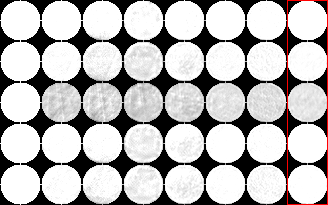
(a) $n_{v}=32,N_{0}$

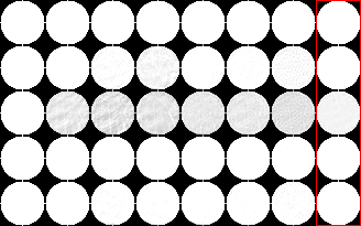
(b) $n_{v}=64,N_{0}$

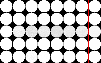
(c) $n_{v}=128,N_{0}$

Figure 13: Visualization of 5 samples of the OOD circle texture reconstruction. From each figure and from left to right, we show the ground truth, FBP, FBPConvNet, DuDoTrans, Learned PD, LEARN, RegFormer and QN-Mixer.

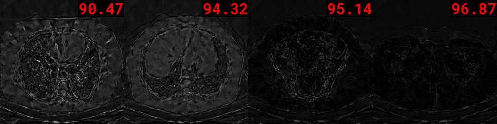
(a)

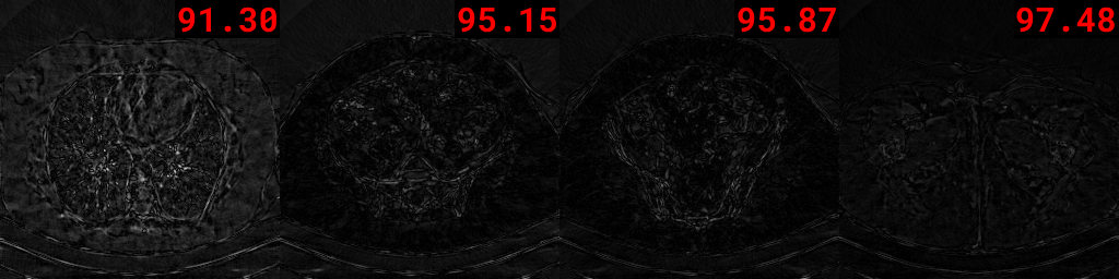
(b)

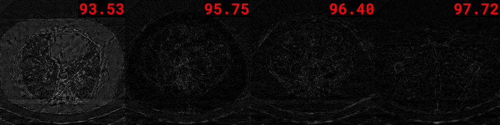
(c)

Figure 14: Reconstruction errors with LEARN, RegFormer, and QN-Mixer using $(n_{v}=32,N_{0})$. Images are ordered left to right by SSIM, with the first column showing the worst reconstruction among $214$ patient images. The second and third columns represent the $1/3$ and $2/3$ percentiles, respectively, and the last column corresponds to the best reconstruction with the highest SSIM.

We present the reconstruction error of QN-Mixer in comparison to LEARN and RegFormer in Fig. 14. The images are organized from left to right based on the SSIM value. As illustrated, our method consistently produces high-quality reconstructions. In the most challenging scenario ($n_{v}=32$) with no added noise, and for the least favorable image, our method achieves a reconstruction with an SSIM of $93.53\%$, maintaining notably satisfactory performance compared to RegFormer with an SSIM of $91.30\%$. For the best reconstruction across all methods, our method achieves an SSIM of $97.72\%$, while RegFormer achieves an SSIM of $97.48\%$. These results demonstrate the robustness of our method when dealing with challenging scenarios.

2.6 Noise Power Spectrum analysis

(a) $n_{v}=32,N_{1}$

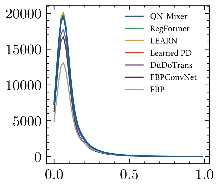
(b) $n_{v}=64,N_{1}$

(c) $n_{v}=128,N_{1}$

Figure 15: Noise Power Spectrum (NPS) Analysis in comparison to state-of-the-art methods. The x-axis represents normalized frequency in cycles per pixel ($\text{px}^{-1}$), and the y-axis represents noise power spectrum ($\text{HU}^{2}\text{px}^{2}$). Display windows are configured as $\left[-1000,800\right]$ HU. Mean and peak frequencies are intricately linked to noise texture, with finer textures correlating to higher mean and peak frequencies in the NPS. Our method exhibits the highest peak frequencies, indicating that our reconstructed images feature the most refined noise texture among all compared methods.

Figure 16: ROIs for NPS Analysis: Red squares denote $20\times 20$ pixel ROIs distributed evenly across two circular regions. The first circle (radius $25$) holds $8$ ROIs, and the second circle (radius $50$) has $20$ ROIs. Both circles, centered at the image center, include a total of $29$ ROIs per image. This standard positioning in the CT community underscores the clinical diagnostic importance of the image center.

We conducted a comprehensive examination of the noise characteristics in our reconstructed images through noise power spectrum (NPS) analysis. NPS serves as a metric, quantifying the magnitude and spatial correlation of noise properties, or textures, within an image. It is derived from the Fourier transform of the spatial autocorrelation function of a zero-mean noise image.

NPS analysis was performed on a configuration of Regions of Interest (ROIs) as depicted in Fig. 16. This process was applied to all $214$ images from the AAPM test set and for three different views ($32$, $64$, and $128$). The average 1D curves were generated by radially averaging the 2D NPS maps, and the results are presented in Fig. 15.

The area under the NPS curve is equal to the square of the noise magnitude. Importantly, the ordering of methods based on noise magnitude corresponds to the ranking observed in our quantitative experiments for PSNR and SSIM in the main text. For example, FBP, which exhibits the lowest noise magnitude, also performs the poorest in terms of PSNR and SSIM. Conversely, our method, with the highest noise magnitude, stands out as the top performer in both PSNR and SSIM metrics. Furthermore, the mean and peak frequencies serve as key indicators of noise texture or “noise grain size”, where higher frequencies denote finer texture. Remarkably, our method showcases superior mean and peak frequencies compared to other methods, suggesting a finer noise texture or smaller grain size.

This alignment with good clinical practice standards reinforces the robust performance of our method in capturing and preserving image details, as supported by both quantitative metrics and noise analysis.

3 Reproducibility

⬇

1class GradientFunction(nn.Module):

2 def __init__(self, regularizer):

3 self.regularizer = regularizer

4 self.lambda = nn.Parameter(torch.zeros(1))

5

6 def forward(self, physics, y, x):

7 y_t = physics.forward_operator(x)

8 # Compute the regularization term

9 reg_x = self.regularizer(x)

10 # Compute the data fidelity term

11 y_dft = y_t - y

12 # Compute the backprojection

13 x_dft = physics.backward_operator(y_dft)

14 g = self.lambda * x_dft + reg_x

15 return g

16

17class QN_Iteration(nn.Module):

18 def __init__(self, gradient_function):

19 self.gradient = gradient_function

20

21 def latent_bfgs (self, h, s_t, z_t):

22 I = torch.eye(len(s_t))

23 rho_t = 1. / torch.dot(z_t, s_t)

24 u_t = I - torch.outer(s_t, z_t) * rho_t

25 d_t = I - torch.outer(z_t, s_t) * rho_t

26 return (torch.matmul(u_t, torch.matmul(h, d_t))

27 + (torch.outer(s_t, s_t) * rho_t))

28

29 def forward(self, physics, encoder, decoder,

30 y, x, h, r, is_last):

31 # Compute latent direction s_t

32 s_t = -torch.matmul(h, r)

33 d = decoder(s_t)

34

35 # Update the reconstruction

36 x = x + d

37 # Return x if it is the last iteration

38 if is_last:

39 return x, h, r

40 else:

41 r_p = encoder(self.gradient(physics, y, x))

42 z_t = r_p - r

43 with torch.no_grad():

44 h = self.latent_bfgs(h, s_t, z_t)

45 return x, h, r_p

Algorithm 3 Minimal QN-Mixer pseudo-code

All our experiments are fully reproducible. While the complete algorithm is already provided in the main paper (see Algorithm 2), we additionally present a PyTorch pseudo-code for enhanced reproducibility in Sec. 3.1. We furnish comprehensive references to all external libraries used in Sec. 3.2. Detailed information regarding the initialization of our model can be found in Sec. 3.3. The precise parameters of our regularizer, Incept-Mixer architecture, are available in Sec. 3.4. We outline the exact data splits utilized across the paper for the AAPM dataset in Sec. 3.5. Lastly, to facilitate the reproduction of our out-of-distribution (OOD) protocol, we provide the pseudo-code in Sec. 3.6.

3.1 QN-Mixer pseudo-code

Our QN-Mixer algorithm is introduced in Algorithm 2, and for improved reproducibility, we present a PyTorch pseudo-code in Algorithm 3. The fundamental concept underlying unrolling networks lies in having a modular gradient function, denoted as $\nabla J({\bm{x}}_{t})$, which can be easily adapted to incorporate various regularization terms. Subsequently, the core element is the unrolling iteration block responsible for updating both the solution ${\bm{x}}_{t}$ and the inverse Hessian approximation ${\bm{H}}_{t}$. The update of the inverse Hessian approximation is executed through the latent BFGS algorithm. Notably, each iteration call takes the physics operator as input, tasked with computing the forward and pseudo-inverse operators for the CT reconstruction problem, along with the gradient encoder and direction decoder, which are shared across all iterations. For a more in-depth understanding, refer to Algorithm 3. Note the employment of torch.no_grad() to inhibit the computation of gradients for the inverse Hessian approximation. Since there is no necessity to compute gradients for this variable, given that it is updated through the latent BFGS algorithm.

Within these two modules, second-order quasi-Newton methods can be seamlessly incorporated by simply modifying the latent BFGS algorithm or the regularization term, offering flexibility to the user.

3.2 External libraries used

We utilized the following external libraries to implement our framework and conduct our experiments:

• Operator Discretization Library (ODL):
  https://github.com/odlgroup/odl

• High-Performance GPU Tomography Toolbox (ASTRA):
  https://www.astra-toolbox.com/

• Medical Imaging Python Library (Pydicom):
  https://pydicom.github.io/

3.3 QN-Mixer’s parameters initialization

To enhance reproducibility, we provide the parameters initialization of QN-Mixer. First, for the gradient function, we initialize the CNNs of Incept-Mixer using the Xavier uniform initialization. The multi-layer perceptron of the MLP-Mixer is initialized with values drawn from a truncated normal distribution with a standard deviation of $0.02$. The $\lambda_{t}$ values are initialized to zero, and the inverse Hessian approximation ${\bm{H}}_{0}$ is initialized with the identity matrix ${\bm{I}}$. Second, for the latent BFGS, both the encoder and decoder CNNs are initialized with the Xavier uniform initialization.

3.4 Incept-Mixer’s architecture

For enhanced reproducibility, we present the architecture of Incept-Mixer in Tab. 10. The Incept-Mixer architecture consists of a sequence of Inception blocks, followed by Mixer blocks. Each Mixer block comprises a channel-mixing MLP and a spatial-mixing MLP. The MLPs are constructed with a fully-connected layer, a GELU activation function, and another fully-connected layer. Ultimately, the regularization value is projected to the same dimension as the input image through a patch expansion layer, which is composed of a fully-connected layer and a CNN layer.

Patient ID	L067	L109	L143	L192	L286	L291	L096	L506	L333	L310
#slices	224	128	234	240	210	343	330	211	244	214
Training	✓	✓	✓	✓	✓	✓	✓	✓	✗	✗
Validation	✗	✗	✗	✗	✗	✗	✗	✗	✓	✗
Testing	✗	✗	✗	✗	✗	✗	✗	✗	✗	✓

Table 9: AAPM dataset split specification. The validation set comprises images from patient L333, and testing utilizes images from patient L310. The images from the remaining patients have been designated for training purposes.

Stage	Layers	#Param (k)	Output size
Input	-	-	$1\times 256\times 256$
InceptionBlock-1	convblock1: conv1-1: K1C16S1P0 prelu1-1 convblock2: conv2-1: K1C16S1P0 prelu2-1 conv2-2: K3C32S1P1 prelu2-2 convblock3: conv3-1: K1C16S1P0 prelu3-1 conv3-2: K5C32S1P2 prelu3-2 convblock4: maxpool4-1: K3S1P1 conv4-1: K1C16S1P0 prelu4-1	17.6	$96\times 256\times 256$
PatchEmbed-2	conv2-1: K4C96S4P0 rearrange2-1: bchw $\rightarrow$ bhwc	$145.5$	$96\times 64\times 64$
MixerLayer-3 $\times(N=2)$	layernorm3-1: D96 rearrange3-1: bhwc $\rightarrow$ bcwh heightmlp3-1: linear3-1: D64O256 gelu3-1 linear3-2: D256O64 rearrange3-2: bcwh $\rightarrow$ bchw widthmlp3-1: linear3-3: D64O256 gelu3-2 linear3-4: D256O64 rearrange3-3: bchw $\rightarrow$ bhwc layernorm3-2: D96 channelmlp3-1: linear3-5: D96O384 gelu3-3 linear3-6: D384O96	$140.8\times 2$	$96\times 64\times 64$
PatchExpand-4	linear4-1: D96O1536 layernorm4-1: D96 conv4-1: K1C1S1P0	$147.7$	$1\times 256\times 256$

Table 10: Incept-Mixer architecture. K-C-S-P represents the kernel, channel, stride, and padding configuration of CNNs, while D-O indicates the input and output dimensions of linear layers.

3.5 AAPM dataset splits

In our experiments, we use the AAPM 2016 Clinic Low Dose CT Grand Challenge public dataset [32], which holds substantial recognition as it was formally established and authorized by the esteemed Mayo Clinic. To ensure the integrity of our evaluation process, we followed the precedent set by [6, 50] and created the training set using data from eight patients, while reserving a separate patient for the testing and validation sets. This approach guarantees that no identity information is leaked during test time. Our specification is presented in Tab. 9.

3.6 Robustness eval. protocol for OOD scenarios

⬇

1def add_circle_ood(img, value=1):

2 h, w = img.shape[::-1][:2]

3 radius = np.random.randint(5, 20)

4 c_x = np.random.randint(radius, w-radius)

5 c_y = np.random.randint(radius, h-radius)

6 center = (c_x, c_y)

7

8 Y, X = np.ogrid[:h, :w]

9 dist_x = (X - center[0])**2

10 dist_y = (Y - center[1])**2

11 dist_from_center = np.sqrt(dist_x + dist_y)

12 mask = dist_from_center <= radius

13 img[0, mask] = value

14 return img

Algorithm 4 add_circle_ood pseudo-code.

In the main paper, we propose a novel protocol specifically crafted for evaluating the effectiveness of reconstruction methods when handling abnormal data lying outside the distribution of the training dataset. Assessing the model’s capability to reconstruct abnormal data holds significant relevance in clinical applications, where patient data may exhibit deviations from the characteristics present in the training data. We strongly advocate for future research endeavors to embrace and employ this protocol as a standard for evaluating the robustness of reconstruction methods. To facilitate the seamless integration of this protocol, we furnish the function’s pseudo-code in Algorithm 4.

4 Limitations

Our approach inherits similar limitations from prior methods [6, 50]. First, our method entails a prolonged optimization time, stemming from the utilization of unrolling reconstruction networks [6, 50], in contrast to post-processing-based denoising methods [17, 45]. While our method represents the fastest unrolling network, there is still a need to address the existing gap. Integrating Limited-memory BFGS into our QN-Mixer framework is an interesting research direction for accelerating training. Second, while we have assessed our method using the well known AAPM low-dose and DeepLesion datasets and compared it with several state-of-the-art methods, the evaluation is conducted on images representing specific anatomical regions (thoracic and abdominal images). The generalizability of our method to a broader range of datasets, which may exhibit diverse characteristics or variations, remains unclear. Third, the acquisition of paired data has always been an important concern in clinic. Combining our approach with unsupervised training framework to overcome this limitation can be an exciting research direction. Finally, the incorporation of actual patient data into our training datasets raises valid privacy concerns. Although the datasets we utilized underwent thorough anonymization and are publicly accessible, exploring a solution that can effectively operate with synthetic data emerges as an intriguing avenue to address this challenge.

5 Notations

We offer a reference lookup table, available in Table 11, containing notations and their corresponding shapes as discussed in this paper.

Notation	Shape	Value(s)	Description
$n_{v}$	$\mathbb{N}^{*}$	$\{32,64,128\}$	The number of projection views
$n_{d}$	$\mathbb{N}^{*}$	512	The number of projection detectors
$h$	$\mathbb{N}^{*}$	$256$	Height of the image
$w$	$\mathbb{N}^{*}$	$256$	Width of the image
$c$	$\mathbb{N}^{*}$	$1$	Channels of the image
$l_{h}$	$\mathbb{N}^{*}$	$64$	Latent height
$l_{w}$	$\mathbb{N}^{*}$	$64$	Latent width
$m=n_{v}\times n_{d}$	$\mathbb{N}^{*}$	$n_{v}\times 512$	Data (sinogram) size
$n=h\times w$	$\mathbb{N}^{*}$	$256\times 256$	Image size
$(l_{h}\cdot l_{w})\times(l_{h}\cdot l_{w})$	$\mathbb{R}$	$(64\cdot 64)\times(64\cdot 64)$	Size of the latent BFGS optimization variable i.e. ${\bm{H}}$
$T$	$\mathbb{N}^{*}$	14	Number of iterations of our method
$t$	$\mathbb{N}$	-	Iteration of the loop in the algorithm
${\bm{y}}$	$n_{v}\times n_{d}$	-	Sparse sinogram
${\bm{A}}$	$\mathbb{R}^{n\times m}$	-	The forward model (i.e. discrete Radon transform)
${\bm{A}}^{\dagger}$	$\mathbb{R}^{m\times n}$	-	The pseudo-inverse of ${\bm{A}}$
${\bm{x}}_{0}$	$\mathbb{R}^{h\times w\times c}$	${\bm{A}}^{\dagger}{\bm{y}}$	Initial reconstruction
$\lambda_{t}$	$\mathbb{R}$	-	Regularization weight at step $t$
$\alpha_{t}$	$\mathbb{R}$	-	Step size (i.e. search step)
${\bm{x}}_{t}$	$\mathbb{R}^{h\times w\times c}$	-	Reconstructed image at iteration $t$
$\nabla_{\bm{x}}J({\bm{x}}_{t})$	$\mathbb{R}^{h\times w\times c}$	-	Gradient value at iteration $t$
${\bm{H}}_{t}$	$\mathbb{R}^{(l_{h}\cdot l_{w})\times(l_{h}\cdot l_{w})}$	-	Approximation of the inverse Hessian matrix at iteration $t$
${\bm{I}}^{n\times n}$	$\mathbb{N}^{n\times n}$	-	Identity matrix of size $n\times n$
${\bm{f}}_{t}$	$\mathbb{R}^{h\times w\times d}$	-	Feature map after the Inception block at iteration $t$
${\bm{e}}_{t}$	$\mathbb{R}^{\frac{h}{p}\times\frac{w}{p}\times d}$	-	MLP-Mixer embeddings
$d$	$\mathbb{R}$	$96$	Depth of features
$p$	$\mathbb{N}^{*}$	$4$	Stride and kernel size in the patchification Conv 2D net
$N$	$\mathbb{N}^{*}$	$2$	Number of stacked Mixer layers
${\mathcal{G}}(\cdot)$	-	-	Learned gradient of the regularization term (i.e. the Incept-Mixer model)
${\mathcal{G}}({\bm{x}}_{t})$	$\mathbb{R}^{h\times w\times c}$	-	Regularization term at step $t$
$\mathcal{E}(\cdot)$	-	-	The gradient encoder
$\mathcal{D}(\cdot)$	-	-	The direction decoder
$k$	$\mathbb{N}^{*}$	$\{2,3,4,5\}$	Number of Downsampling stacks in the encoder
${\bm{f}}_{\mathcal{E}}=2^{k}$	$\mathbb{N}^{*}$	$\{4,8,16,32\}$	Downsampling factor of the gradient in the encoder
$w_{l}={w}/{{\bm{f}}_{\mathcal{E}}}$	$\mathbb{N}^{*}$	$\{64,32,16,8\}$	Number of columns of the down-sampled gradient
$h_{l}={h}/{{\bm{f}}_{\mathcal{E}}}$	$\mathbb{N}^{*}$	$\{64,32,16,8\}$	Number of rows of the down-sampled gradient
${\bm{r}}_{t}=\mathcal{E}(\nabla_{{\bm{x}}}J({\bm{x}}_{t}))$	$\mathbb{R}^{l_{h}\cdot l_{w}}$	-	Latent representation of the gradient
$s_{t}=-{\bm{H}}_{t}{\bm{r}}_{t}$	$\mathbb{R}^{l_{h}\cdot l_{w}}$	-	Direction in the latent space
$\rho_{t}={({\bm{z}}_{t}^{\mathsf{T}}{\bm{s}}_{t})}^{-1}$	$\mathbb{R}^{l_{h}\cdot l_{w}}$	-	BFGS divider variable
$N_{0}$	-	-	Zero noise added to the sinogram
$N_{1}$	-	-	5% Gaussian noise, $1\times 10^{6}$ intensity Poisson noise
$N_{2}$	-	-	5% Gaussian noise, $5\times 10^{5}$ intensity Poisson noise

Table 11: Lookup table of notations and hyperparameters used in the paper.

References

- Adler and Öktem [2018] Jonas Adler and Ozan Öktem. Learned primal-dual reconstruction. IEEE TMI, 37:1322–1332, 2018.
- Arie and Avinash [1984] Andersen Arie and Kak Avinash. Simultaneous algebraic reconstruction technique (SART): a superior implementation of the art algorithm. Ultrasonic imaging, 6:81–94, 1984.
- Ashish et al. [2017] Vaswani Ashish, Shazeer Noam, Parmar Niki, Uszkoreit Jakob, Jones Llion, Gomez Aidan N, Kaiser Lukasz, and Polosukhin Illia. Attention is all you need. In NeurIPS, 2017.
- Avinash and Malcolm [2001] Kak Avinash and Slaney Malcolm. Principles of Computerized Tomographic Imaging. Society for Industrial and Applied Mathematics, 2001.
- Chen et al. [2017] Hu Chen, Yi Zhang, Mannudeep K. Kalra, Feng Lin, Yang Chen, Peixi Liao, Jiliu Zhou, and Ge Wang. Low-dose CT with a residual encoder-decoder convolutional neural network. IEEE TMI, 36:2524–2535, 2017.
- Chen et al. [2018] Hu Chen, Yi Zhang, Yunjin Chen, Junfeng Zhang, Weihua Zhang, Huaiqiang Sun, Yang Lv, Peixi Liao, Jiliu Zhou, and Ge Wang. LEARN: Learned experts’ assessment-based reconstruction network for sparse-data CT. IEEE TMI, 37:1333–1347, 2018.
- Cheng et al. [2020] Weilin Cheng, Yu Wang, Hongwei Li, and Yuping Duan. Learned full-sampling reconstruction from incomplete data. IEEE TCI, pages 945–957, 2020.
- Chengbin et al. [1993] Peng Chengbin, Rodi William L., and M. Nafi Toksöz. A Tikhonov Regularization Method for Image Reconstruction, pages 153–164. Springer US, 1993.
- Davidon [1991] William C. Davidon. Variable metric method for minimization. SIAM Journal on Optimization, 1:1–17, 1991.
- Dianlin et al. [2022] Hu Dianlin, Zhang Yikun, Liu Jin, Luo Shouhua, and Chen Yang. DIOR: Deep iterative optimization-based residual-learning for limited-angle CT reconstruction. IEEE TMI, pages 1778–1790, 2022.
- Fabian et al. [2022] Zalan Fabian, Berk Tinaz, and Mahdi Soltanolkotabi. HUMUS-Net: Hybrid unrolled multi-scale network architecture for accelerated MRI reconstruction. In NeurIPS, 2022.
- Fletcher [1987] Roger Fletcher. Practical Methods of Optimization. John Wiley & Sons, New York, NY, USA, 1987.
- Gartner et al. [2023] Erik Gartner, Luke Metz, Mykhaylo Andriluka, C. Daniel Freeman, and Cristian Sminchisescu. Transformer-based Learned Optimization. In CVPR, pages 11970–11979, 2023.
- Ghani and Karl [2018] Muhammad Usman Ghani and W. Clem Karl. Deep learning-based sinogram completion for low-dose CT. In 2018 IEEE 13th Image, Video, and Multidimensional Signal Processing Workshop, pages 1–5, 2018.
- Harshit et al. [2018] Gupta Harshit, Jin Kyong Hwan, Nguyen Ha Q., McCann Michael T., and Unser Michael. CNN-based projected gradient descent for consistent CT image reconstruction. IEEE TMI, 37:1440–1453, 2018.
- Hu et al. [2020] Dianlin Hu, Jin Liu, Tianling Lv, Qianlong Zhao, Yikun Zhang, Guotao Quan, Juan Feng, Yang Chen, and Limin Luo. Hybrid-domain neural network processing for sparse-view CT reconstruction. IEEE TRPMS, 5:88–98, 2020.
- Jin et al. [2017] Kyong Hwan Jin, Michael T. McCann, Emmanuel Froustey, and Michael Unser. Deep convolutional neural network for inverse problems in imaging. IEEE TIP, 26:4509–4522, 2017.
- Jinxi et al. [2021] Xiang Jinxi, Dong Yonggui, and Yang Yunjie. FISTA-Net: Learning a fast iterative shrinkage thresholding network for inverse problems in imaging. IEEE TMI, 40:1329–1339, 2021.
- Jorge and J [2006] Nocedal Jorge and Wright Stephen J. Quasi-Newton methods. Numerical optimization, 75:135–163, 2006.
- Kawata and Nalcioglu [1985] Satoshi Kawata and Orhan Nalcioglu. Constrained iterative reconstruction by the conjugate gradient method. IEEE TMI, 4:65–71, 1985.
- Kobler et al. [2020] Erich Kobler, Alexander Effland, Karl Kunisch, and Thomas Pock. Total deep variation for linear inverse problems. In CVPR, pages 7546–7555, 2020.
- Lee et al. [2018] Hoyeon Lee, Jongha Lee, Hyeongseok Kim, Byungchul Cho, and Seungryong Cho. Deep-neural-network-based sinogram synthesis for sparse-view CT image reconstruction. IEEE TRPMS, 3:109–119, 2018.
- Lee et al. [2020] Minjae Lee, Hyemi Kim, and Hee-Joung Kim. Sparse-view CT reconstruction based on multi-level wavelet convolution neural network. Physica Medica, 80:352–362, 2020.
- Li et al. [2022] Runrui Li, Qing Li, Hexi Wang, Saize Li, Juanjuan Zhao, Yan Qiang, and Long Wang. DDPTransformer: Dual-domain with parallel transformer network for sparse view CT image reconstruction. IEEE TCI, pages 1–15, 2022.
- Li et al. [2023] Zilong Li, Chenglong Ma, Jie Chen, Junping Zhang, and Hongming Shan. Learning to distill global representation for sparse-view ct. In ICCV, pages 21196–21207, 2023.
- Lin et al. [2019] Wei-An Lin, Cheng Liao, Haofu Peng, Xiaohang Sun, Jingdan Zhang, Jiebo Luo, Rama Chellappa, and Zhou S. Kevin. DuDoNet: Dual domain network for CT metal artifact reduction. In CVPR, pages 10512–10521, 2019.
- Liu and Luo [2022] Chengchang Liu and Luo Luo. Quasi-newton methods for saddle point problems. In NeurIPS, 2022.
- Liu et al. [2021] Ze Liu, Yutong Lin, Yue Cao, Han Hu, Yixuan Wei, Zheng Zhang, and Stephen Lin Baining Guo. Swin transformer: Hierarchical vision transformer using shifted windows. In ICCV, pages 9992–10002, 2021.
- Loshchilov and Hutter [2017] Ilya Loshchilov and Frank Hutter. Decoupled Weight Decay Regularization. arXiv preprint arXiv:1711.05101, 2017.
- Lunz et al. [2018] Sebastian Lunz, Ozan Öktem, and Carola-Bibiane Schönlieb. Adversarial regularizers in inverse problems. In NeurIPS, 2018.
- Macleod [1963] Cormack Allan Macleod. Representation of a function by its line integrals, with some radiological applications. Journal of Applied Physics, 34:2722–2727, 1963.
- McCollough [2016] C. McCollough. TU-FG-207A-04: Overview of the low dose CT grand challenge. Medical Physics, 43:3759–3760, 2016.
- Metz et al. [2022] Luke Metz, C. Daniel Freeman, James Harrison, Niru Maheswaranathan, and Jascha Sohl-Dickstein. Practical tradeoffs between memory, compute, and performance in learned optimizers. arXiv preprint arXiv:2203.11860, 2022.
- Miller and Schauer [1983] Donald L. Miller and David Schauer. The alara principle in medical imaging. Philosophy, 44:595–600, 1983.
- Mukherjee et al. [2021] Subhadip Mukherjee, Marcello Carioni, Ozan Öktem, and Carola-Bibiane Schönlieb. End-to-end reconstruction meets data-driven regularization for inverse problems. In NeurIPS, 2021.
- Öktem et al. [2014] Ozan Öktem, Jonas Adler, Holger Kohr, and The ODL Team. Operator discretization library (ODL), 2014.
- Radon [1917] Johann Radon. über die bestimmung von funktionen durch ihre integralwerte längs gewisser mannigfaltigkeiten. Berichte über die Verhandlungen der Königlich-Sächsischen Akademie der Wissenschaften zu Leipzig, 69:262–277, 1917.
- Robin et al. [2022] Rombach Robin, Blattmann Andreas, Lorenz Dominik, Esser Patrick, and Ommer Björn. High-resolution image synthesis with latent diffusion models. In CVPR, pages 10684–10695, 2022.
- Rui et al. [2017] Liu Rui, He Lu, Luo Yan, and Yu Hengyong. Singular value decomposition-based 2D image reconstruction for computed tomography. Journal of X-ray science and technology, 25:113–134, 2017.
- Shaohua et al. [2014] Niu Shaohua, Gao Yan, Bian Zhaoying, Huang Jing, Chen Wufan, Yu Hengyong, Liang Zhengrong, and Ma Jianhua. Sparse-view x-ray CT reconstruction via total generalized variation regularization. PMB, 59:2997–3017, 2014.
- Sriram et al. [2020] Anuroop Sriram, Jure Zbontar, Tullie Murrell, Aaron Defazio, C. Lawrence Zitnick, Nafissa Yakubova, Florian Knoll, and Patricia Johnson. End-to-End variational networks for accelerated MRI reconstruction. In MICCAI, pages 64–73, 2020.
- Szegedy et al. [2015] Christian Szegedy, Wei Liu, Yangqing Jia, Pierre Sermanet, Scott Reed, Dragomir Anguelov, Dumitru Erhan, and Vincent Vanhoucke Andrew Rabinovich. Going deeper with convolutions. In CVPR, pages 1–9, 2015.
- Tolstikhin et al. [2021] Ilya Tolstikhin, Neil Houlsby, Alexander Kolesnikov, Lucas Beyer, Xiaohua Zhai, Thomas Unterthiner, Jessica Yung, Andreas Peter Steiner, Daniel Keysers, Jakob Uszkoreit, Mario Lucic, and Alexey Dosovitskiy. MLP-mixer: An all-MLP architecture for vision. In NeurIPS, 2021.
- Tsutomu and Yukio [2018] Gomi Tsutomu and Koibuchi Yukio. Use of a Total Variation minimization iterative reconstruction algorithm to evaluate reduced projections during digital breast tomosynthesis. BioMed Research International, 2018:1–14, 2018.
- Wang et al. [2022] Ce Wang, Kun Shang, Haimiao Zhang, Qian Li, and S. Kevin Zhou. DuDoTrans: Dual-domain transformer for sparse-view CT reconstruction. In Machine Learning for Medical Image Reconstruction, pages 84–94. Springer International Publishing, 2022.
- Wang et al. [2008] Ge Wang, Hengyong Yu, and Bruno De Man. An outlook on X-ray CT research and development. Medical Physics, 35:1051–1064, 2008.
- Wang et al. [2019] Jiaxi Wang, Li Zeng, Chengxiang Wang, and Yumeng Guo. ADMM-based deep reconstruction for limited-angle CT. PMB, 64, 2019.
- Weiwen et al. [2021] Wu Weiwen, Hu Dianlin, Niu Chuang, Yu Hengyong, Vardhanabhuti Varut, and Wang Ge. DRONE: Dual-domain residual-based optimization network for sparse-view CT reconstruction. IEEE TMI, 40:3002–3014, 2021.
- Wu et al. [2017] Dufan Wu, Kyungsang Kim, Georges El Fakhri, and Quanzheng Li. Iterative low-dose ct reconstruction with priors trained by artificial neural network. IEEE TMI, 36:2479–2486, 2017.
- Xia et al. [2022] Wenjun Xia, Ziyuan Yang, Qizheng Zhou, Zexin Lu, Zhongxian Wang, and Yi Zhang. Transformer-based iterative reconstruction model for sparse-view CT reconstruction. In MICCAI, 2022.
- Yan et al. [2018] Ke Yan, Xiaosong Wang, Le Lu, and Ronald M. Summers. DeepLesion: Automated mining of large-scale lesion annotations and universal lesion detection with deep learning. Journal of Medical Imaging, 5:036501, 2018.
- Yi et al. [2023] Zhang Yi, Chen Hu, Xia Wenjun, Chen Yang, Liu Baodong, Liu Yan, Sun Huaiqiang, and Zhou Jiliu. LEARN++: Recurrent dual-domain reconstruction network for compressed sensing CT. IEEE TRPMS, 7:132–142, 2023.
- Yu-Jung et al. [2018] Tsai Yu-Jung, Bousse Alexandre, Ehrhardt Matthias J., Stearns Charles W., Ahn Sangtae, Hutton Brian F., Arridge Simon, and Thielemans Kris. Fast quasi-newton algorithms for penalized reconstruction in emission tomography and further improvements via preconditioning. IEEE TMI, 37:1000–1010, 2018.
- Zhang et al. [2018] Zhicheng Zhang, Xiaokun Liang, Xu Dong, Yaoqin Xie, and Guohua Cao. A sparse-view CT reconstruction method based on combination of DenseNet and deconvolution. IEEE TMI, 37:1407–1417, 2018.