Universal energy-speed-accuracy trade-offs in driven nonequilibrium systems

Abstract

Physical systems driven away from equilibrium by an external controller dissipate heat to the environment; the excess entropy production in the thermal reservoir can be interpreted as a “cost” to transform the system in a finite time. The connection between measure theoretic optimal transport and dissipative nonequilibrium dynamics provides a language for quantifying this cost and has resulted in a collection of “thermodynamic speed limits”, which argue that the minimum dissipation of a transformation between two probability distributions is directly proportional to the rate of driving. Thermodynamic speed limits rely on the assumption that the target probability distribution is perfectly realized, which is almost never the case in experiments or numerical simulations. Here, we address the ubiquitous situation in which the external controller is imperfect. As a consequence, we obtain a lower bound for the dissipated work in generic nonequilibrium control problems that 1) is asymptotically tight and 2) matches the thermodynamic speed limit in the case of optimal driving. We illustrate these bounds on analytically solvable examples and also develop a strategy for optimizing minimally dissipative protocols based on optimal transport flow matching, a generative machine learning technique. This latter approach ensures the scalability of both the theoretical and computational framework we put forth. Crucially, we demonstrate that we can compute the terms in our bound numerically using efficient algorithms from the computational optimal transport literature and that the protocols that we learn saturate the bound.

1 Introduction

Trade-offs involving dissipation, control, and fluctuations are a unifying feature among the few universal results that constrain nonequilibrium dynamics. While fluctuation theorems [13, 24, 23], thermodynamic uncertainty relations [4, 18], and thermodynamic speed limits [2] all have broad applicability, for many physical systems the bounds computed from these fundamental relations are too weak for inference of the dissipation rate [19] or are difficult to compute directly in many-body systems [12].

Recent efforts to adopt a purely geometric perspective on nonequilibrium dynamics are creating an opportunity for new analytical and computational approaches that more precisely constrain and quantify dissipation, even far from equilibrium. Foundational work in the partial differential equations literature [21] revealed a deep connection between dissipation and optimal transport theory; in particular, the relaxation to equilibrium described by a Fokker-Planck equation follows a Wasserstein geodesic and the geometry of the geodesic relates to relaxational entropy production. Aurell [2] made the connection explicit in the language of stochastic thermodynamics and showed that the total entropy production of a driven nonequilibrium transformation can be directly expressed in terms of the Wasserstein distance. This relation, in turn, leads to thermodynamic speed limits [29, 41].

Unfortunately, the difficulty of solving high-dimensional optimal transport problems, both analytically and numerically, limits the applicability of this conceptually elegant approach. Currently, it is both difficult to identify external control protocols that drive a system accurately towards a fixed target distribution and also minimize dissipation. Existing strategies for minimum dissipation protocol optimization either require a linear response approximation [36, 14, 33, 17] or necessitate exact knowledge of the optimal transport mapping [11].

There has been tremendous recent progress in computational optimal transport [15, 31], but these techniques have not yet been brought to bear on problems in nonequilibrium physics. In particular, state-of-the-art generative modeling techniques based on ideas from the theory of measure transport closely resemble the theoretical paradigm of optimal nonequilibrium control. Generative machine learning techniques provide new and exciting opportunities to solve high-dimensional control problems on which classical numerical methods fail [17, 22, 7]. Here we leverage an approach to generative modeling called flow matching [39, 26, 1, 25] that explicitly formulates a machine learning algorithm in the language of measure transport to approximately solve nonequilibrium optimal control problems. We demonstrate that this framework yields control forces that accurately drive many-particle systems towards arbitrary targets.

Because the solutions obtained by any computational approach will be necessarily approximate, we also refine the theoretical formulation of the thermodynamic speed limits to account for the imperfect control protocols. In doing so, we introduce a thermodynamically interpretable notion of “accuracy”; this bears interesting and provocative parallels to quantities like the statistical precision of generalized currents that appear in thermodynamic uncertainty relations [4], but the definition we use is not tied to a specific observable. The most significant contribution of our work is the strikingly general bound that we obtain by formalizing the notion of accurate control, which unveils a universal trade-off among energy dissipation, speed of driving, and accuracy of control.

2 Optimal transport distance and dissipation

Throughout, we consider finite-time nonequilibrium optimal control problems in which we seek to drive a system with initial probability density $\rho_{0}$ to a final density $\rho_{*}$ at time $t.$ We consider a classical system with coordinates $\boldsymbol{x}\in\Omega\subset\mathbb{R}^{d}$, and assume throughout that trajectories of this system evolve according to the overdamped Langevin equation

$$\text{d}\boldsymbol{X}_{t}=b(\boldsymbol{X}_{t},t)\text{d}t+\sqrt{2\beta^{-1}}\text{d}\boldsymbol{W}_{t},\quad\boldsymbol{X}_{0}=\boldsymbol{x}.$$ (1)

Here the drift $b:\mathbb{R}^{d}\to\mathbb{R}^{d}$ generically contains both conservative and non-conservative forcing terms, $\beta^{-1}=k_{\rm b}T$, and $\boldsymbol{W}$ is a $d$-dimensional Wiener process. Following the conventions of stochastic thermodynamics [35], we write the single trajectory entropy production as

$$\Delta S_{\rm tot}[\boldsymbol{X}_{[0,t_{\rm tot}]}] =\Delta S_{\rm sys}-\beta Q[\boldsymbol{X}_{[0,t_{\rm tot}]}]$$ (2)

$$=\log\frac{\rho_{t_{\rm tot}}(\boldsymbol{X}_{t_{\rm tot}})}{\rho_{0}(\boldsymbol{X}_{0})}-\beta\int_{0}^{t_{\rm tot}}b(\boldsymbol{X}_{s},s)\circ\text{d}\boldsymbol{X}_{s}.$$

The average system entropy change $\Delta S_{\rm sys}$ is a state function only involving the initial density $\rho_{0}$ and the final density $\rho_{t_{\rm tot}}$. The second term in (2) is a time-symmetric Stratonovich integral, which is conventionally interpreted to be proportional to the heat flow along the trajectory, $Q[\boldsymbol{X}_{[0,t]}]$. Remarkably, as shown by Aurell [2], taking an expectation over trajectories, the average total entropy production can be bounded by an optimal transport distance between the initial and final distributions

$$\Delta S_{\rm tot}\geq t_{\rm tot}^{-1}\mathcal{W}_{2}^{2}(\rho_{0},\rho_{*}),$$ (3)

where $\mathcal{W}_{2}$ denotes the Wasserstein-2 distance between $\rho_{0}$ and $\rho_{*}$. In principle, this optimal transport distance can be computed by minimizing the $L_{2}$ distance

$$\int_{\Omega}|\boldsymbol{x}-T(\boldsymbol{x})|^{2}\rho_{0}(\boldsymbol{x})\text{d}\boldsymbol{x}$$ (4)

over transport plans $T$ satisfying

$$\rho_{*}(\boldsymbol{x})\mathsf{d}\boldsymbol{x}=T\#\rho_{0}(\boldsymbol{x})\mathsf{d}\boldsymbol{x}\equiv\frac{\rho_{0}(T^{-1}(\boldsymbol{x}))}{\det\bigl{(}\nabla T(T^{-1}(\boldsymbol{x}))\bigr{)}}\text{d}\boldsymbol{x}.$$ (5)

This formulation immediately leads to a number of useful insights; first, it clearly establishes a lower bound on the entropy production rate for systems driven to a target state in a finite time, a result explored in several recent works [29, 41, 16, 42]. Secondly, the dissipation is minimal when the optimal transport map $T\equiv T_{*}$ is known exactly.

While the optimal transport formulation is a mathematically elegant and conceptually clear framing that yields a finite-time refinement of the Second Law, the assumption of (5)—that the final distribution is perfectly realized—cannot be imposed easily for arbitrary target densities $\rho_{*}$. Indeed, in many systems that we may want to control, the realizable transport plans will be limited by the set of external couplings available. Of course, this means that the minimizer of (4) may not be reached.

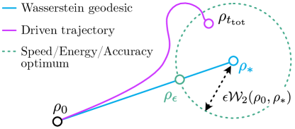
Figure 1: The minimum dissipation required to produce an $\epsilon$-accurate distribution $\rho_{\epsilon}$ is derived based on purely geometric criteria. This argument leads to a generic energy-speed-accuracy trade-off (6). Constant speed geodesics in Wasserstein space are depicted as straight lines in the schematic.

Failing to reach the target distribution $\rho_{*}$ alters the constraint on the total dissipation; trivially, if we make no change to the distribution, there is no excess entropy production from the control. A more productive setting to consider is one in which we closely realize the target distribution, but do not satisfy exactly the constraint (5). Suppose we set a target “accuracy” which we measure in the Wasserstein distance: we say that a distribution $\rho$ is $\epsilon$-accurate if $\mathcal{W}_{2}(\rho,\rho_{*})\leq\epsilon\mathcal{W}_{2}(\rho_{0},\rho_{*})$, as illustrated in Fig. 1. We now ask about the cost of getting close to the target distribution; in other words, we address how the lower bound on the dissipation is influenced by the accuracy parameter $\epsilon$.

The optimal controller will follow a Wasserstein geodesic at all times, as illustrated in Fig. 1. Because $\mathcal{W}_{2}$ is a proper distance metric on the space of probability densities we consider here, it is straightforward to see via the triangle inequality that the minimal dissipation to produce an $\epsilon$-accurate distribution $\rho$ at time $t_{\rm tot}$ must result from following the geodesic between $\rho_{0}$ and $\rho_{*}$. A physically realizable external coupling that we use to drive a given system may not follow this optimal trajectory at every point in time. As a result, we immediately obtain the bound

$$t_{\rm tot}\Delta S_{\rm tot}\geq(1-\epsilon)^{2}\mathcal{W}_{2}^{2}(\rho_{0},\rho_{*})\text{ where }\epsilon=\mathcal{W}_{2}(\rho_{t_{\rm tot}},\rho_{*})/\mathcal{W}_{2}(\rho_{0},\rho_{*}),$$ (6)

where the right-hand side is a purely geometric quantity depending on only the initial distance, the target distance, and the $\epsilon$-accurate density. In other words, the total entropy production is lower bounded by the square of the Wasserstein distance between the initial distribution and the idealized target multiplied by a factor that accounts for the inaccuracy of a realistic controller.

Remarkably, this result provides a tight and generic energy-speed-accuracy trade-off: 1) increasing accuracy at fixed duration increases minimum dissipation; 2) increasing duration at fixed accuracy decreases minimum dissipation; 3) for nearly optimal driving either increasing accuracy or increasing speed will in turn increase the total dissipation. Throughout, we refer to (6) as the ESA bound. Importantly, this lower bound is sharp when the controller is optimal, i.e., following a $\mathcal{W}_{2}$-geodesic leads to saturation of this bound because the Wasserstein distance provides an exact measure of the total entropy production. The total dissipation of the controlled process may exceed the lower bound when the control is imperfect, and how precisely the controller realizes the $\mathcal{W}_{2}$-geodesic provides a measure of the quality of the lower bound. We find that the bound provides a useful constraint on the dissipative costs of control arbitrarily far from equilibrium and further provides important guidance for optimizing minimally dissipative controllers using generative machine learning techniques.

We exemplify the ESA bound (6) first on exactly solvable models, highlighting the way in which the bound differs from thermodynamic speed-limits. We then turn to high-dimensional examples for which the optimal transport problem cannot be solved exactly; we demonstrate that carefully learning protocols with generative optimal transport flow matching yields controllers that saturate the ESA bound. This latter result emphasizes a computational pathway to the design of low dissipation nonequilibrium control, which has important applications in many domains [20, 33, 30, 40].

3 Analytically solvable particle systems

3.1 Finite time protocols for equilibrium to equilibrium driving

To illustrate the energy-speed-accuracy bound, we first consider a parametric Hamiltonian $U(\boldsymbol{x},\boldsymbol{\lambda})$ in equilibrium with a thermal reservoir at inverse temperature $\beta$, so that the stationary distribution with fixed parameters $\boldsymbol{\lambda}$ is given by

$$\rho^{\rm eq}_{\boldsymbol{\lambda}}(\boldsymbol{x})=\text{exp}\left[-\beta(U(\boldsymbol{x},\boldsymbol{\lambda})-F_{\boldsymbol{\lambda}})\right],$$ (7)

where $F_{\boldsymbol{\lambda}}=-\beta^{-1}\log Z(\beta,\boldsymbol{\lambda})$ and $Z$ denotes the partition function. To drive the system from an initial stationary distribution $\rho^{\rm eq}_{\boldsymbol{\lambda}_{0}}$ to a final distribution $\rho^{\rm eq}_{\boldsymbol{\lambda}_{*}}$, we vary $\boldsymbol{\lambda}$ according to a prescribed protocol $\boldsymbol{\lambda}(t)$ halting at a finite time $t_{\rm tot}$ such that $\boldsymbol{\lambda}(0)=\boldsymbol{\lambda}_{0}$ and $\boldsymbol{\lambda}(t_{\rm tot})=\boldsymbol{\lambda}_{*}$. For a transformation beginning and ending in equilibrium, we write the total entropy production associated with a control protocol, $\Delta S_{\rm tot}=\beta W-\beta\Delta F$, in terms of the expected work along a trajectory [35],

$$W=\int_{0}^{t_{\rm tot}}\text{d}t\ \dot{\boldsymbol{\lambda}}\cdot\left\langle\partial_{\boldsymbol{\lambda}}U(\boldsymbol{X},\boldsymbol{\lambda})\right\rangle_{\rho_{t}},$$ (8)

where $\left\langle\cdot\right\rangle_{\rho_{t}}$ denotes an expectation taken with respect to the instantaneous density $\rho_{t}.$ In the slow driving limit, the instantaneous distribution and equilibrium distributions correspond $\rho_{t}=\rho^{\rm eq}_{\boldsymbol{\lambda}(t)}$, and the entropy production is identically zero. In practice, driving protocols are carried out in a finite time $t_{\rm tot}<\infty$, resulting in an excess dissipation $\Delta S_{\rm tot}=\Delta S^{\rm drive}_{\rm tot}+\Delta S^{\rm relax}_{\rm tot}>0$, which we decompose into contributions from driving and relaxation dynamics. Since $\Delta S^{\rm relax}_{\rm tot}\geq 0$, the bound (6) yields a lower bound on the total entropy production. For fixed $\epsilon$-accurate protocols, the entropy production associated to the relaxation, given by $\Delta S^{\rm relax}_{\rm tot}=D_{\rm KL}(\rho_{t_{\rm tot}}||\rho_{\boldsymbol{\lambda}_{*}}^{\rm eq})$ is upper bounded by a $t_{\rm tot}$-independent constant [38], such that for short driving times the ESA bound is tight. The bound (6) highlights, in particular, the irrelevance of the Wasserstein speed limit (3) for finite time protocols that do not reach the target distribution.

Linearly driven Ornstein-Uhlenbeck process

We exemplify the observation above using an analytically tractable example. We consider the excess dissipation of a one-dimensional particle in a linearly displaced harmonic trap with fixed stiffness [34, 6]. The particle, initially at thermal equilibrium and distributed according to $\rho^{\rm eq}_{\lambda_{0}}\propto\text{exp}\left[-\beta k(x-\lambda_{0})^{2}/2\right]$, is driven towards a target distribution $\rho_{*}^{\rm eq}\propto\text{exp}\left[-\beta k(x-\lambda_{*})^{2}/2\right]$ along a finite time linear protocol

$$\lambda_{t}=\lambda_{0}+(\lambda_{*}-\lambda_{0})\frac{t}{t_{\rm tot}}$$ (9)

at constant temperature. The equation of motion for the particle position is given by

$$\text{d}X_{t}=-k(X_{t}-\lambda_{t})\text{d}t+\sqrt{2\beta^{-1}}\text{d}W_{t};\quad X_{0}\sim\rho_{\lambda_{0}}^{\rm eq}$$ (10)

and a straightforward calculation shows that the instantaneous distribution of $X_{t}$ is a Gaussian with mean and variance given by

$$\left\langle X_{t}\right\rangle=\frac{\mu_{0}(1+k(t_{\rm tot}-t))+\mu_{*}(kt-1)}{kt_{\rm tot}}+\frac{e^{-kt}(\mu_{*}-\mu_{0})}{kt_{\rm tot}}$$ (11)

$$\left\langle(X_{t}-\left\langle X_{t}\right\rangle)^{2}\right\rangle=\beta k.$$

Because the variance of $\rho^{\rm eq}_{\lambda_{0}}$ coincides with that of the target, the free energy difference vanishes and

$$\Delta S_{\rm tot}=\beta W=\beta\frac{\left[t_{\rm tot}-k^{-1}(e^{-kt_{\rm tot}}-1)\right](\lambda_{0}-\lambda_{*})^{2}}{t_{\rm tot}^{2}}.$$ (12)

What is more, for Gaussian distributions, the optimal transport distance can be computed in closed form $\mathcal{W}_{2}^{2}(\rho_{t_{\rm tot}},\rho_{\lambda_{*}})=(\left\langle X_{t_{\rm tot}}\right\rangle-\lambda_{*})^{2}$, from which one obtains the accuracy parameter $\epsilon$ exactly. Fig. 2 illustrates both the Wasserstein speed-limit (3) and the ESA bound (6) along with numerical simulations of the dynamics (10).

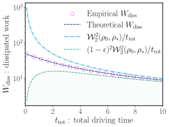
Figure 2: Total entropy production along the linear driving protocol from $\lambda_{0}=0$ to $\lambda_{*}=10.0$. The stiffness parameter and inverse temperature are constant along the trajectory, with $\beta=k=1.0$.

Even though the complexity of this model is low, the speed-limit (3) does not constrain the entropy production on the fastest timescales because the target distribution is not exactly realized. On the other hand, the ESA bound (6) provides a clear lower bound across all driving times.

3.2 Finite-time approximate control of many-body systems

Saturating the speed limit constraint requires a protocol that can drive the system along the constant speed Wasserstein geodesic. For systems consisting of many interacting particles such precise control necessitates specifically coupling to every degree of freedom of the distribution. Realistic control protocols may instead only couple to a fraction of the system’s degrees of freedom, limiting accuracy. The result is a discrepancy between the distribution at the stopping time of the protocol and target distribution; as we show in the following calculation, the ESA bounds precisely relate this discrepancy to the dissipation.

Partially driven interacting particle system.

To probe the effect of imperfect control, we consider a system $\boldsymbol{X}\in\mathbb{R}^{N}$ consisting of $N$ interacting particles in contact with a thermal reservoir, and subject to a quadratic interaction potential $\mathcal{U}(\boldsymbol{X})$

$$\mathcal{U}(\boldsymbol{X})=\frac{\alpha}{2}\sum_{i\neq j}(X_{i}-X_{j})^{2},$$ (13)

where $\alpha$ sets the strength of the interaction. The system is initially prepared such that $\rho_{0}(\boldsymbol{X})\sim\mathcal{N}(\mathbf{0},\mathbb{I})$, and we set the target distribution to be $\rho_{*}(\boldsymbol{X})\sim\mathcal{N}(\mu\mathbf{1},\mathbb{I})$ with $\mu>0$. In the case of perfect control over the system, the instantaneous distribution $\rho_{t}$ is an interpolating Gaussian $\rho_{t}\sim\mathcal{N}(\mu t/t_{\rm tot}\mathbf{1},\mathbb{I})$. However, to elucidate the effect of partial control, we only drive a fraction $f$ of the total set of particles. The controlled particles are optimally driven between the source and target marginals via

$$\text{d}X_{t}^{\rm c}=\left[\frac{\mu}{t_{\rm tot}}-\beta^{-1}\left(X_{t}^{\rm c}-\mu\frac{t}{t_{\rm tot}}\right)\right]\text{d}t+\sqrt{2\beta^{-1}}\text{d}W_{t}$$ (14)

resulting in a Gaussian distribution $\rho_{t}^{c}\sim\mathcal{N}(\mu t/t_{t_{\rm tot}},1)$. The uncontrolled degrees of freedom are dragged along due to the pairwise interactions (shown in Fig. 3(a)), and the corresponding equation of motion reads

$$\text{d}X_{t}^{\alpha,i}=-\alpha\left[\sum_{i\neq j}(X_{t}^{\alpha,i}-X_{t}^{j})\right]\text{d}t+\sqrt{2\beta^{-1}}\text{d}W_{t}.$$ (15)

We recast the dynamics (14) and (15) of this partially controlled system as a as a multidimensional Ornstein-Ulhenbeck process, and provide the complete time dependent distribution in Appendix A. Importantly, the instantaneous means $\mu_{t}^{\alpha}=\tfrac{(\exp(-\alpha fNt)-1)\mu+\alpha fNt\mu}{\alpha fNt_{\rm tot}}$ and $\mu_{t}^{\rm c}=\mu t/t_{\rm tot}$ qualitatively illustrate the link between accuracy and dissipation; indeed, in the highly dissipative strong interaction limit, it is clear that $\mu_{t}^{\alpha}\to\mu_{t}^{\rm c}$.

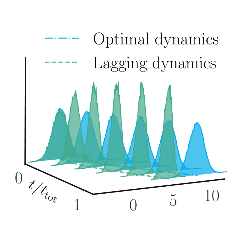
(a) Accuracy

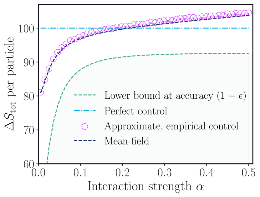
(b) Dissipation

Figure 3: (a) Instantaneous snapshots of the partially controlled system (14)-(15). The interaction term induces a deformation of the complete distribution, as the interacting particles try and follow the driven ones.(b) Total entropy production for the partially controlled system (14)-(15) with $N=100$, $f=0.8$, $\mu=10.0$, $t_{\rm tot}=1.0$ and $\beta=1.0$. Since the system’s distribution remains Gaussian at all times, both the system entropy change and the accuracy $\epsilon$ can be computed exactly. The greened-out zone is inaccessible at the corresponding $\epsilon$ accuracy.

We now make this link explicit by numerically evaluating the ESA bound for this system. We compute the empirical entropy production $\Delta S_{\rm tot}=\frac{1}{2}\log\left(|\text{Det}\ \boldsymbol{\Sigma}_{t_{\rm tot}}|\right)-\beta Q[\boldsymbol{X}_{[0,t_{\rm tot}]}]$, where the mean dissipated heat $Q$ is defined as in equation (2). Additionally, we carry out a mean-field treatment of the coupled dynamics (14) and (15)—see Appendix A—yielding excellent agreement with numerical experiments, as shown in Fig. 3(b). As evidenced by the increasing lower bound in, higher interaction strengths yield more accurate control.

In turn, the associated energetic cost increases in tandem with $\alpha$ and potentially will exceed the Wasserstein speed limit. While the ESA bound plateaus as the interaction strength $\alpha$ increases, the dissipation continues to rise without evident bound. The observations of Fig. 3(b) provide an important reminder that only idealized controllers follow the constant speed geodesic, and a typical protocol may be far from this case. Importantly, the ESA bound remains valid in settings where the speed limits fail.

4 High-dimensional control and flow matching

We now turn to high dimensional systems, for which exact solutions to the optimal transport problem are generally unknown. As a result, designing minimally dissipative control forces to drive a system from $\rho_{0}$ to $\rho_{*}$ becomes challenging. In the following, we leverage a recently developed machine learning framework for generative modeling [1, 25, 26] that poses sampling as a transport problem. With an appropriate formulation, this framework can be extended to provide an algorithmic toolkit for computational optimal transport in high dimensions [32, 39].

These recent extensions of continuous normalizing flows [25], dubbed Optimal Transport Flow Matching (OTFM) suggest that minimizing the $\mathcal{W}_{2}$ length along the generative pathway aids optimization and model performance for image generation tasks [32, 39]. An optimized flow field using the OTFM objectives results in trajectories that closely resemble constant speed Wasserstein geodesics. We show here that this approach naturally fits the paradigm of stochastic thermodynamics and provides an appealing route to determining optimal controllers even for high-dimensional physical systems.

4.1 Learning optimal control forces

The OTFM framework builds upon the more general CNF framework [8], which proposes to learn a flow field $u_{t}(x)$ such that the solution $\psi_{t}(x)$ to the ODE

$$\text{d}\psi_{t}(x)=u_{t}(\psi_{t}(x))\text{d}t$$ (16)

with initial condition $\psi_{0}(x)=x\sim\rho_{0}$, transports $\rho_{0}$ to $\rho_{*}$ in time $t_{\rm tot}$. Enforcing optimal transport constraints along the probability pathway has been shown to give good performance on standard machine learning tasks like image generation. The flow field is determined by minimizing the objective

$$\mathcal{L}_{\rm CFM}\left[\theta\right]=\mathbb{E}_{t\sim\mathcal{U}(0,1),\rho_{t}(x|z),q(z)}||u^{\theta}(t,x)-v_{t}(x|z)||^{2}_{2},$$ (17)

where the conditional distribution $\rho_{t}(x|z)$ and training field $v_{t}(x|z)$ are such that

$$\rho_{t}(x|z)=\mathcal{N}\left[(1-t)x_{0}+tx_{1},\sigma\right],$$ (18)

$$v_{t}(x|z)=(x_{1}-x_{0}),$$

and the $x_{0}$ and $x_{1}$ are sampled from the Wasserstein optimal coupling $\pi^{\rm OT}$ between $\rho_{0}$ and $\rho_{*}$. Following [25], we provide an extended description of the OTFM procedure in Appendix B. While the algorithm (17)-(18) actually transports the convolution $\rho_{0}*\mathcal{N}(0,\sigma)$ onto $\rho_{*}*\mathcal{N}(0,\sigma)$, the small $\sigma$ limit is particularly enlightening. In that case, it can be shown that the instantaneous distribution $\rho_{t}$ closely follows the constant speed Wasserstein geodesic between $\rho_{0}$ and $\rho_{*}$. When this is the case, the learned flow field $u_{t}^{\theta}$ realizes the optimal dynamical control from source to target.

Optimizing control protocols.

Exploiting the deep connection between optimal transport and stochastic thermodynamics, we now tailor OTFM to nonequilibrium control problems. To motivate the general approach, we consider as in Sec. 3.1 a particle in contact with a thermal bath, whose dynamics are given by the one-dimensional overdamped Langevin equation

$$\text{d}X_{t}=b(X_{t},t)\text{d}t+\sqrt{2\beta^{-1}}\text{d}W_{t},$$ (19)

and we seek a control force $b$ to drive the system from $\rho_{0}$ to $\rho_{*}$ with minimum dissipation. The corresponding Fokker-Planck equation is given by

$$\partial_{t}\rho_{t}=-\nabla\left[(b-\beta^{-1}\nabla\log\rho_{t})\rho_{t}\right],\hskip 10.0pt\rho_{t=0}=\rho_{0}$$ (20)

and the least dissipative protocol drives $\rho_{t}$ along the constant speed Wasserstein geodesic between source and target. We learn an optimal driving force $b=v^{\theta}+\beta^{-1}s^{\theta}$, where $v^{\theta}$ minimizes the conditional OTFM objective (17) and $s^{\theta}$ cancels out the score $\nabla\log\rho_{t}$. Importantly, it can be shown ([1] and Appendix B) that the score associated to the OTFM pathway (18) is the unique minimizer of the objective function

$$\mathcal{L}_{\rm score}\left[s\right]=\mathbb{E}_{t\sim\mathcal{U}(0,1),\rho_{t}(x|z),q(z)}||s-{\rm noise}(x,z,t)||^{2}_{2},$$ (21)

$${\rm noise}(x,z,t)=\sigma^{-1}\left[x-tx_{1}-(1-t)x_{0}\right].$$

Consequently, both $v^{\theta}$ and $s^{\theta}$ can be trained concurrently to produce an optimal control $b^{*}$.

This methodology relies on a number of approximations. First, even assuming perfect learning, the OTFM pathway is not exactly the Wasserstein geodesic between source and target due to the convolution of the initial and target distributions with a Gaussian. More importantly, accurate sampling from the optimal coupling $\pi^{OT}$ is not feasible in practice, and one needs to resort to approximate methods, such as the Sinkhorn algorithm [15] or direct empirical estimates of optimal transport distance. Importantly, these approaches still provide scalable and controlled approximations of the optimal coupling [28]. Moreover, we emphasize that even if potentially inaccurate, the control $b^{*}$ allows for dissipation and accuracy gains, whose interplay is quantified by the general ESA bound (6).

4.2 Applications to multimodal distributions and interacting particle systems

Bimodal optimal driving

The significant impact of using an empirical OT coupling on the resulting dissipation is evident even in minimal models. Consider driving a two-dimensional particle in contact with a thermal reservoir between two non-overlapping Gaussian mixtures

$$\rho_{0}(\boldsymbol{x})=\frac{1}{2}\left[p_{1}(\boldsymbol{x})+p_{2}(\boldsymbol{x})\right],\hskip 10.0pt\rho_{*}(\boldsymbol{x})=\frac{1}{2}\left[p_{3}(\boldsymbol{x})+p_{4}(\boldsymbol{x})\right],\hskip 10.0ptp_{i}\sim\mathcal{N}\left(\boldsymbol{\mu}_{i},\boldsymbol{\Sigma}_{i}\right)$$ (22)

$$\boldsymbol{\mu}_{1}=\begin{bmatrix}6\\ 0\end{bmatrix}\hskip 10.0pt\boldsymbol{\mu}_{2}=\begin{bmatrix}-6\\ 0\end{bmatrix}\hskip 10.0pt\boldsymbol{\mu}_{3}=\begin{bmatrix}-10\\ -10\end{bmatrix}\hskip 10.0pt\boldsymbol{\mu}_{4}=\begin{bmatrix}10\\ 10\end{bmatrix}\hskip 10.0pt\boldsymbol{\Sigma}_{1}=\boldsymbol{\Sigma}_{2}=\mathbb{I}_{2},\hskip 10.0pt\boldsymbol{\Sigma}_{3}=\boldsymbol{\Sigma}_{4}=\mathbb{I}_{2}\times 0.1.$$

We employ two distinct CFM training strategies: $b^{\times}$ is trained with source and target samples drawn independently, while $b^{\rm OT}$ is trained on an approximate OT coupling of $\rho_{0}$ and $\rho_{*}$ obtained from finite size samples. Next, we generate trajectories by integrating the Langevin dynamics (19) and display samples from the resulting distributions $\rho^{\rm OT}$ and $\rho^{\times}$ on figure 4(a).

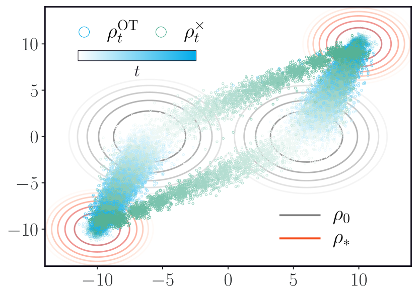
(a) Accuracy

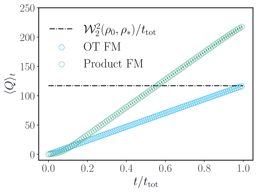
(b) Dissipation

Figure 4: (a) Two dimensional samples from the source and target distribution, as well as dynamical samples generated from the learned controllers $b^{\times}$ and $b^{\rm OT}$. Both controllers display satisfying performance, but the space-time trajectories of the driven samples are very different.(b) Empirical dissipated heat along the dynamics (19) with $\beta=1.0$. The highly dissipative nature of the trajectories associated to $b^{\times}$ stems from the excess displacement illustrated on Fig (4(a)).

Both strategies produce protocols that approximately reach the target distribution, but the associated dynamics are thermodynamically distinct, as reflected in the cumulative dissipated heat shown in figure 4(b). Indeed, the OT trained distribution clearly flows along the Wasserstein geodesic, as indicated by the constant entropy production rate and the total dissipated heat which saturates the classical speed energy limit. On the other hand, the controller trained on independent samples yields greater dissipation, emphasizing the significance of attending to the optimal control pathway.

Scalable control of active interacting particles

We can directly employ control strategies based on OTFM to build minimum dissipation protocols in complex physical systems. We consider the problem of “switching” a system of $\boldsymbol{X}_{t}$ of $N$ quorum sensing active particles (QSAP) [37] in a bistable potential from one metastable state to the other; the dynamics of this system are described in detail in Appendix C. In the absence of any control, QSAP particles settle in the metastable states, and transitions are enhanced by the activity, as depicted in figure 5(a), a dynamics we deem thermalizing, in parallel to equilibrium dynamics in the same potential.

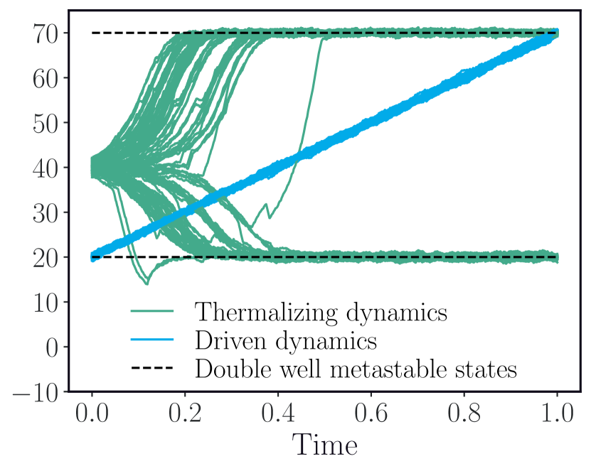
(a)

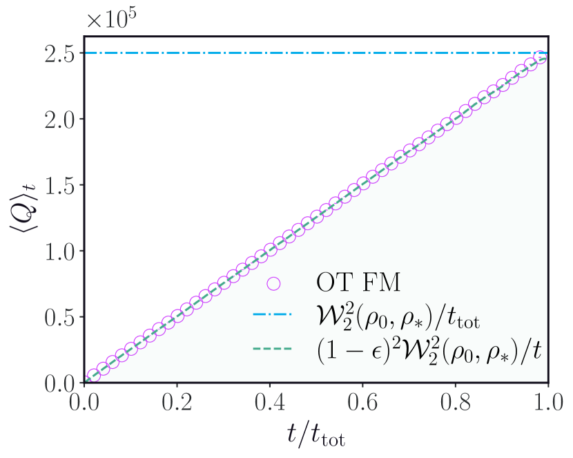
(b) Dissipation

Figure 5: (a) Thermalizing and driven dynamics for a cloud of $N=100$ QSAP with parameter values $a=20,b=40,c=70,A=0.03,v_{0}=300,\ell=1,\lambda=10,t_{\rm tot}=1,\beta=0.2$. Specific QSAP behavior is apparent in the thermalizing dynamics, with clear jagged trajectories corresponding to run and tumble type motion. (b) The observed heat at intermediate times from the ESA bound (green dashed line) compared with OTFM (circles). The Wasserstein speed limit is shown in blue.

Though transition rates are increased by the run and tumble motion between metastable states, a collective transition remains unlikely. In the following we design a control force $f^{(c)}(\boldsymbol{X},t)$ to drive the interacting particle system from one well to the other in a finite time $t_{\rm tot}$, and discuss the relevance of the ESA bound in that case. Since the stationary distribution of the QSAP system is not known, we define the source and target distributions to be the Gaussian expansion of the activity-free equilibrium distribution near the well centers

$$\rho_{0}(\boldsymbol{X})\sim\mathcal{N}\left(\mathbf{1}a,\mathbb{I}\frac{\beta^{-1}}{U^{\prime\prime}(a)}\right),\hskip 10.0pt\rho_{*}(\boldsymbol{X})\sim\mathcal{N}\left(\mathbf{1}c,\mathbb{I}\frac{\beta^{-1}}{U^{\prime\prime}(c)}\right).$$ (23)

As a result, the optimal control force $f^{(c)}=\eta^{(c)}+F^{(c)}+v^{(c)}$ decomposes in three terms: $\eta^{(c)}(\boldsymbol{X}_{t})\equiv-\eta(\boldsymbol{X}_{t})$ cancels the interaction; $F^{(c)}\equiv\nabla U(\boldsymbol{X})$ cancels the conservative force and $v^{(c)}$ maintains the instantaneous distribution on the Wasserstein geodesic between $\rho_{0}$ and $\rho_{*}$. Since perfect control may not be reached by physical controllers, we illustrate the accuracy gap by representing $\eta^{(c)}$ and $F^{(c)}$ as neural networks trained on uncontrolled trajectory data D. Learned control forces perform particularly well, as the dynamical total dissipated heat is close to optimal. Fig. 5(b) shows the average dissipated heat along approximate control trajectories, including both the corresponding ESA bound and also the classical energy speed limit.

5 Conclusion

Recent results that link control, dissipation, and speed [36, 11, 29, 16] are built on deep mathematical connections between optimal transport theory and physical dynamics [21, 3]. Away from the idealized setting in which the exact optimal mapping can be identified and realized, thermodynamic speed limits do not necessarily provide a meaningful constraint on dissipation. Here, we demonstrate that an approach built on the geometry of optimal transport still supports precise lower bounds that not only relate dissipation and speed, but also quantify the thermodynamic cost of highly accurate control. We show the the ESA bound tightly constrain the dissipation in analytically solvable models, where the optimal controller can be constructed exactly.

Applications of optimal transport theory have been limited in scope for physical systems, perhaps due to the lack of scalable computational methods, but synergistic developments in generative machine learning are breaking down these computational barriers. Our results, which use empirical estimates of Wasserstein distances together with optimal transport flow-matching provide strong evidence that high-dimensional controllers can be constructed which are nearly optimal thermodynamically.

Here, our primary focus has been optimal control of diffusive classical systems. Extensions of the thermodynamic connection between OT and stochastic thermodynamics to Markov jump processes [27] and open quantum systems [9, 5, 11] require further development and investigation. Furthermore, the provocative connection between our results, which relate dissipation, speed, and accuracy, with the thermodynamic uncertainty relations that indicate a universal trade-off between dissipation and the precision of fluctuations [4, 18] merits further investigation, as well.

Appendix A Solution to the Multidimensional Coupled OU Processes

The coupled equations (14) and (15) can be recast as the following multidimensional SDE

$$\text{d}\boldsymbol{X}_{t}=-\left[\boldsymbol{A}\boldsymbol{X}+\boldsymbol{b}\right]\text{d}t+\sqrt{2\beta^{-1}}\text{d}\boldsymbol{W}_{t}$$ (24)

with time dependent drift

$$\boldsymbol{A}=\left[\begin{array}[]{cc}\beta^{-1}\mathbb{I}&\mathbf{0}\\ &\\ \lx@intercol\hfil\alpha\mathbf{U}\hfil\lx@intercol\end{array}\right],\hskip 10.0pt\mathbf{U}\in\mathbb{R}^{(1-f)N\times N}\hskip 5.0pt{\rm s.t.}\hskip 5.0pt\left\{\begin{array}[]{l}\mathbf{U}_{ij}=-1\\ \mathbf{U}_{ii}=N-1\end{array}\right.,\hskip 10.0pt\boldsymbol{b}=\begin{bmatrix}\mathbf{1}\\ \mathbf{0}\end{bmatrix}\frac{\mu}{t_{\rm tot}}(1+\beta^{-1}t),$$ (25)

from which one obtains the instantaneous distribution $\rho_{t}(\boldsymbol{X})\sim\mathcal{N}(\boldsymbol{\mu}_{t},\boldsymbol{\Sigma}_{t})$

$$\boldsymbol{\mu}_{t}=\begin{bmatrix}\mathbf{1}_{fN}\times\mu_{t}^{\rm c}\\ \mathbf{1}_{(1-f)N}\times\mu_{t}^{\alpha}\end{bmatrix},\hskip 10.0pt\mu_{t}^{\rm c}=\mu t/t_{\rm tot},\hskip 10.0pt\mu_{t}^{\alpha}=\frac{(e^{-\alpha fNt}-1)\mu+\alpha fNt\mu}{\alpha fNt_{\rm tot}},$$ (26)

$$\boldsymbol{\Sigma}_{t}=e^{-\boldsymbol{A}t}e^{-\boldsymbol{A}^{T}t}+2\beta^{-1}\int_{0}^{t}e^{-\boldsymbol{A}(t-s)}e^{-\boldsymbol{A}^{T}(t-s)}\text{d}s.$$

In turn, we compute the Wasserstein distance between $\rho_{t_{\rm tot}}$ and $\rho_{*}$ using the Bures metric [31],

$$\mathcal{W}_{2}^{2}(\rho_{t_{\rm tot}},\rho_{*})=||\boldsymbol{\mu}_{t_{\rm tot}}-\mu\mathbf{1}||^{2}_{2}+\text{tr}\left[(\boldsymbol{\Sigma}_{t_{\rm tot}}^{1/2}-\mathbb{I})^{2}\right].$$ (27)

which is obtained via numerical integration of equation (27). In the large $N$ limit, a mean-field approximation of (14) and (15) can be employed to decouple the dynamics of the interacting particles. This approximation yields

$$\text{d}X_{t}^{\alpha}=-\alpha\left[fN(X_{t}^{\alpha}-\mu_{t}^{\rm c})+(1-f)N(X_{t}^{\alpha}-\mu_{t}^{\alpha})\right]\text{d}t+\sqrt{2\beta^{-1}}\text{d}W_{t}$$ (28)

such that the instantaneous marginal distribution of an interacting particle has mean $\mu_{t}^{\alpha}$ and variance

$$\Sigma_{t}^{\alpha}=e^{-2\alpha Nt}+\frac{1-e^{-2\alpha Nt}}{\beta\alpha N}.$$ (29)

Consequently, the mean-field total dissipation is obtained as $\Delta S^{\rm MF}_{\rm tot}=fN\Delta S^{\rm c}_{\rm tot}+(1-f)N\Delta S^{\alpha}_{\rm tot}$, and gives excellent agreement relative to numerical experiments, as shown in Fig. 3(b). Higher interaction strengths yield more accurate control, which is evident from the increasing lower bound in Fig. 3(b).

Appendix B Optimal Transport Flow Matching

Most of the following expressions are directly extracted from [25] and reproduced here for the sake of completeness. Given source and target distributions $\rho_{0}$ and $\rho_{*}$, flow matching methods build upon the general Continuous Normalizing Flow (CNF) framework [8] which proposes to learn a flow field $u_{t}(x)$ such that the solution $\psi_{t}(x)$ to the ODE

$$\text{d}\psi_{t}(x)=u_{t}(\psi_{t}(x))\text{d}t$$ (30)

with initial condition $\psi_{0}(x)=x\sim\rho_{0}$, transports $\rho_{0}$ to $\rho_{*}$ in time $t_{\rm tot}$. Specifically, the instantaneous distribution $\rho_{t}=\psi_{t}\#\rho_{0}$ evolves according to

$$\partial_{t}\rho_{t}=-\nabla\left[u_{t}\rho_{t}\right],$$ (31)

and one seeks to learn $u_{t}$ with the endpoint constraint $\rho_{t_{\rm tot}}=\rho_{*}$. While initial CNF algorithms train on likelihood estimation, requiring multiple backward and forward ODE passes [8], the formulation of conditional flow matching (CFM) algorithms offer simulation free training objectives for $u_{t}$ without ODE solves. In this context, the general FM objective is given by

$$\mathcal{L}_{\rm FM}\left[\theta\right]=\mathbb{E}_{t\sim\mathcal{U}(0,1),\rho_{t}(x)}||v^{\theta}(t,x)-u_{t}(x)||^{2}_{2}$$ (32)

where $v^{\theta}$ regresses the sought after flow field. Of course, neither $u_{t}$ nor $\rho_{t}$ are known, and (32) is intractable as such. However these difficulties can be bypassed by introducing an alternative CFM objective

$$\mathcal{L}_{\rm CFM}\left[\theta\right]=\mathbb{E}_{t\sim\mathcal{U}(0,1),\rho_{t}(x|z),q(z)}||v^{\theta}(t,x)-u_{t}(x|z)||^{2}_{2}$$ (33)

where the latent variable $z$, sampled from some distribution $q(z)$, and the conditional distribution $\rho_{t}(x|z)$ are chosen such that

$$\rho_{t}(x)=\int\rho_{t}(x|z)q(z)\text{d}z,$$ (34)

and $\rho_{t}(x|z)$ is generated by a conditional flow field $u_{t}(x|z)$ from initial datum $\rho_{0}(x|z)$. Crucially, both $\mathcal{L}_{\rm CFM}$ and $\mathcal{L}_{\rm FM}$ share the same minimizer. As a result, suitable choices of $z$ and $\rho_{t}(x|z)$ make the objective (33) explicit; in particular, the OTFM objective is obtained by considering the specific case

$$\rho_{t}(x|z)=\mathcal{N}\left[(1-t)x_{0}+tx_{1},\sigma\right]$$ (35)

$$u_{t}(x|z)=(x_{1}-x_{0})$$

where $x_{0}$ and $x_{1}$ are sampled from the Wasserstein optimal coupling $\pi^{\rm OT}$ between $\rho_{0}$ and $\rho_{*}$.

We now show how to numerically evaluate the score $s_{t}(x)\equiv\nabla\log\rho_{t}$ associated to the OTFM conditional pathway (35). To simplify notations, we set $t_{\rm tot}=1$. The essential idea is to consider the OTFM framework in the light of the stochastic interpolant framework independently developed in [1]. Specifically, the conditional distribution

$$\rho_{t}(x|z)=\mathcal{N}((1-t)x_{0}+tx_{1},\sigma)$$ (36)

is the instantaneous conditional distribution of the stochastic interpolant

$$x_{t}=(1-t)x_{0}+tx_{1}+\sigma z,\hskip 10.0ptz\sim\mathcal{N}(0,1),\hskip 10.0ptt\in[0,1],$$ (37)

conditioned on a given pair $(x_{0},x_{1})$ sampled from the optimal coupling $\pi^{\rm OT}$. Following the stochastic interpolant framework, the instantaneous distribution $\rho_{t}$ of $x_{t}$ obeys the following continuity equation

$$\partial_{t}\rho_{t}=-\nabla\left[u_{t}\rho_{t}\right]$$ (38)

where $u_{t}$ is the unique minimizer of the objective function

$$\mathcal{L}^{u}_{\rm SI}[\hat{u}]=\mathbbm{E}_{(x_{0},x_{1})\sim\pi^{\rm OT}}||\hat{u}-(x_{1}-x_{0})||_{2}^{2},$$ (39)

recovering the OTFM result (35). However, the stochastic interpolant framework also allows for the explicit characterization of the score — see equation (2.15) of [1] — as the unique minimizer of

$$\mathcal{L}^{s}_{\rm SI}[\hat{s}]=\mathbbm{E}_{\left\{\begin{subarray}{c}(x_{0},x_{1})\sim\pi^{\rm OT},t\sim\mathcal{U}(0,1)\\ z\sim\mathcal{N}(0,1),x=(1-t)x_{0}+tx_{1}+\sigma z\end{subarray}\right\}}||\hat{s}(x)+z\sigma^{-1}||_{2}^{2},$$ (40)

which is strictly equivalent to the loss function (21).

Appendix C QSAP Dynamics

We here provide a few details on the dynamical implementation of the QSAP system discussed in the main text. The particles evolve according to the over-damped Langevin equation

$$\text{d}X^{i}_{t}=\left[-\nabla U(X^{i}_{t})+\eta^{i}(\boldsymbol{X}_{t})\right]\text{d}t+\sqrt{2\beta^{-1}}\text{d}W_{t},$$ (41)

where $U$ is taken to be quartic and asymmetric, such that the resulting force is given by

$$-\nabla U(X_{t})=-A(X_{t}-a)(X_{t}-b)(X_{t}-c)$$ (42)

with $a<c$ the respective positions of the two metastable states of the potential. The particles interact via the quorum sensing mechanism embedded in the interaction kernel $\eta$:

$$\eta^{i}(\boldsymbol{X}_{t})=\mathbbm{1}\left\{\underset{j\neq i}{\rm min}|X_{t}^{i}-X_{t}^{j}|>\ell\right\}\times v_{0}\times\zeta^{i}_{t}$$ (43)

where $\zeta^{i}_{t}$ is a telegraph process oscillating between $1$ and $-1$ with rate $\lambda$, $\ell$ is the interaction cutoff, and $v_{0}$ denotes the speed of a particle during an active phase. In words, the QSAP showcase a simple relaxation behavior when in close range of other particles, and adopt a run and tumble motion when isolated. In turn, the controlled equation of motion for one particle is given by

$$\text{d}X^{i}_{t}=\left[-\nabla U(X^{i}_{t})+\eta^{i}(\boldsymbol{X}_{t})+f^{(c),i}(\boldsymbol{X}_{t},t)\right]\text{d}t+\sqrt{2\beta^{-1}}\text{d}B_{t},$$ (44)

and a sample trajectory is shown in Fig. 5(a). The mean dissipated heat is computed using the Stratonovitch rule as

$$\left\langle Q\right\rangle_{t_{\rm tot}}=\left\langle\beta\int_{0}^{t_{\rm tot}}\sum_{i=1}^{N=100}\left(\left[-\nabla U(X^{i}_{t})+\eta^{i}(\boldsymbol{X}_{t})+f^{(c),i}(\boldsymbol{X}_{t},t)\right]\circ\text{d}X^{i}_{t}\right)\right\rangle,$$ (45)

averaged over $10^{2}$ trajectories.

Appendix D Training

In this Appendix, we provide details on the various training architectures used throughout the main text. Table 1 recapitulates the values of the hyperparameters we used for the training protocols. Below, we provide further information on training routines, in particular the dataset construction

D.1 OTFM - Fig 4(a)

To train the OTFM field $b^{\rm OT}$ on the objective (17), we first generate $N$ independent samples $x_{0}^{i}$ and $x_{1}^{i}$ from $\rho_{0}$ and $\rho_{*}$ respectively. We then use the python POT optimal transport library to obtain empirical optimal coupling sample pairs $(x_{0}^{\rm OT},x_{1}^{\rm OT})_{1\leq i\leq N}$ which are used as inputs to carry out the OTFM optimization.

D.2 QSAP - Fig 5(a)

To control QSAP trajectories and illustrate the optimal driving procedure, we learn approximate representations of the external force $F^{(c)}\equiv-\nabla U$ and quorum sensing kernel $\eta^{(c)}\equiv\eta$ introduced in the main text.

• $\mathbf{F^{(c)}}$ — Because the external force acts on each particle independently, we parametrize the network as $F^{(c)}:\mathbbm{R}^{2}\to\mathbbm{R}$. We optimize the MSE loss between $F^{(c)}$ and the ground truth $\nabla U$ on independent samples $(t,x)_{1\leq i\leq N}$ generated from $t\sim\mathcal{U}(0,t_{\rm tot}),\ x\sim\mathcal{N}(t,2.0)$. We make this choice to help learn the control force in the viscinity of the desired controlled trajectory.

• $\mathbf{\boldsymbol{\eta}^{(c)}}$ — The quorum sensing kernel is a simple scaled Heaviside function. We parameterize the network as $\eta^{(c)}:\mathbbm{R}\to[0,1]$ and train on the MSE loss with the ground truth ${\rm Heavi}_{\ell}$, where $\ell$ is the QS cutoff parameter. The training data is drawn independently from a Normal distribution. Note that during inference, the control force is taken to be $\mathbbm{1}_{x>1/2}\circ\eta^{(c)}$ to recover the binary nature of the QS mechanism.

Table 1: Training protocol details

	Network architecture	Optimizer	Scheduler	Samples	Batch Size	Epochs
Fig. 4(a)
$b^{\rm OT}$	MLP with 1 hidden layer, 256 neurons and ReLU activation	Adam(lr=$3.10^{-4}$)	ReduceLROnPlateau(patience=5,factor=0.8,min_lr=$10^{-6}$)	$10^{4}$	64	$10^{3}$
$b^{\times}$	MLP with 1 hidden layer, 256 neurons and ReLU activation	Adam(lr=$3.10^{-4}$)	ReduceLROnPlateau(patience=5,factor=0.8,min_lr=$10^{-6}$)	$10^{5}$	64	$5.10^{3}$
Fig. 5(a)
$\eta^{(c)}$	MLP with 1 hidden layer, 512 neurons and ReLU activation	Adam(lr=$10^{-3}$)	ReduceLROnPlateau(patience=5,factor=0.8,min_lr=$10^{-6}$)	$10^{4}$	64	$10^{3}$
$F^{(c)}$	MLP with 1 hidden layer, 512 neurons and ReLU activation	Adam(lr=$10^{-3}$)	ReduceLROnPlateau(patience=5,factor=0.8,min_lr=$10^{-6}$)	$10^{4}$	64	$10^{3}$

References

- [1] Michael S. Albergo and Eric Vanden-Eijnden. Building normalizing flows with stochastic interpolants. In The eleventh international conference on learning representations, ICLR 2023, kigali, rwanda, may 1-5, 2023. OpenReview.net, 2023. tex.bibsource: dblp computer science bibliography, https://dblp.org tex.timestamp: Fri, 30 Jun 2023 14:55:53 +0200.
- [2] Erik Aurell, Krzysztof Gawedzki, Carlos Mejía-Monasterio, Roya Mohayaee, and Paolo Muratore-Ginanneschi. Refined Second Law of Thermodynamics for Fast Random Processes. Journal of Statistical Physics, 147(3):487–505, May 2012.
- [3] Erik Aurell, Carlos Mejía-Monasterio, and Paolo Muratore-Ginanneschi. Optimal Protocols and Optimal Transport in Stochastic Thermodynamics. Physical Review Letters, 106(25):250601, June 2011.
- [4] Andre C Barato and Udo Seifert. Thermodynamic Uncertainty Relation for Biomolecular Processes. Phys. Rev. Lett., 114(15):158101, April 2015.
- [5] Simon Becker and Wuchen Li. Quantum Statistical Learning via Quantum Wasserstein Natural Gradient. Journal of Statistical Physics, 182(1):7, January 2021.
- [6] Valentin Blickle and Clemens Bechinger. Realization of a micrometre-sized stochastic heat engine. Nature Physics, 8(2):143–146, February 2012. Number: 2 Publisher: Nature Publishing Group.
- [7] Nicholas M. Boffi and Eric Vanden-Eijnden. Deep learning probability flows and entropy production rates in active matter, September 2023.
- [8] Ricky T. Q. Chen, Yulia Rubanova, Jesse Bettencourt, and David K Duvenaud. Neural ordinary differential equations. In S. Bengio, H. Wallach, H. Larochelle, K. Grauman, N. Cesa-Bianchi, and R. Garnett, editors, Advances in neural information processing systems, volume 31. Curran Associates, Inc., 2018.
- [9] Yongxin Chen, Tryphon T. Georgiou, and Allen Tannenbaum. Matrix Optimal Mass Transport: A Quantum Mechanical Approach. IEEE Transactions on Automatic Control, 63(8):2612–2619, August 2018. Conference Name: IEEE Transactions on Automatic Control.
- [10] Yongxin Chen, Tryphon T. Georgiou, and Allen Tannenbaum. Optimal Transport for Gaussian Mixture Models. IEEE Access, 7:6269–6278, 2019.
- [11] Shriram Chennakesavalu and Grant M. Rotskoff. Unified, Geometric Framework for Nonequilibrium Protocol Optimization. Physical Review Letters, 130(10):107101, March 2023. Publisher: American Physical Society.
- [12] Shriram Chennakesavalu, David J. Toomer, and Grant M. Rotskoff. Ensuring thermodynamic consistency with invertible coarse-graining. The Journal of Chemical Physics, 158(12):124126, March 2023. Publisher: American Institute of Physics.
- [13] Gavin E. Crooks. Entropy production fluctuation theorem and the nonequilibrium work relation for free energy differences. Physical Review E, 60(3):2721–2726, September 1999.
- [14] Gavin E Crooks. Measuring Thermodynamic Length. Phys. Rev. Lett., 99(10):100602, September 2007.
- [15] Marco Cuturi. Sinkhorn distances: Lightspeed computation of optimal transport. In C. J. C. Burges, L. Bottou, M. Welling, Z. Ghahramani, and K. Q. Weinberger, editors, Advances in neural information processing systems 26, pages 2292–2300. Curran Associates, Inc., 2013.
- [16] Andreas Dechant, Shin-ichi Sasa, and Sosuke Ito. Geometric decomposition of entropy production in out-of-equilibrium systems. Physical Review Research, 4(1):L012034, March 2022. tex.ids= dechant_geometric_2021 arXiv: 2109.12817.
- [17] Megan C. Engel, Jamie A. Smith, and Michael P. Brenner. Optimal Control of Nonequilibrium Systems through Automatic Differentiation. Physical Review X, 13(4):041032, November 2023. Publisher: American Physical Society.
- [18] Todd R Gingrich, Jordan M Horowitz, Nikolay Perunov, and Jeremy L England. Dissipation Bounds All Steady-State Current Fluctuations. Phys. Rev. Lett., 116(12):120601, March 2016.
- [19] Todd R Gingrich, Grant M Rotskoff, and Jordan M Horowitz. Inferring dissipation from current fluctuations. J. Phys. A: Math. Theor., 50(18):184004, April 2017.
- [20] C. Jarzynski. Targeted free energy perturbation. Physical Review E, 65(4):046122, April 2002. arXiv: cond-mat/0109461.
- [21] Richard Jordan, David Kinderlehrer, and Felix Otto. The Variational Formulation of the Fokker–Planck Equation. SIAM Journal on Mathematical Analysis, 29(1):1–17, January 1998.
- [22] George Em Karniadakis, Ioannis G. Kevrekidis, Lu Lu, Paris Perdikaris, Sifan Wang, and Liu Yang. Physics-informed machine learning. Nature Reviews Physics, 3(6):422–440, June 2021.
- [23] Jorge Kurchan. Fluctuation theorem for stochastic dynamics. J. Phys. A, 31(16):3719–3729, 1998.
- [24] Joel L. Lebowitz and Herbert Spohn. A Gallavotti–Cohen-Type Symmetry in the Large Deviation Functional for Stochastic Dynamics. Journal of Statistical Physics, 95(1):333–365, April 1999.
- [25] Yaron Lipman, Ricky T. Q. Chen, Heli Ben-Hamu, Maximilian Nickel, and Matthew Le. Flow Matching for Generative Modeling. September 2022.
- [26] Xingchao Liu, Chengyue Gong, and Qiang Liu. Flow Straight and Fast: Learning to Generate and Transfer Data with Rectified Flow. September 2022.
- [27] Jan Maas. Gradient flows of the entropy for finite Markov chains. Journal of Functional Analysis, 261(8):2250–2292, October 2011.
- [28] Gonzalo Mena and Jonathan Niles-Weed. Statistical bounds for entropic optimal transport: sample complexity and the central limit theorem. In Advances in Neural Information Processing Systems, volume 32. Curran Associates, Inc., 2019.
- [29] Muka Nakazato and Sosuke Ito. Geometrical aspects of entropy production in stochastic thermodynamics based on Wasserstein distance. Physical Review Research, 3(4):043093, November 2021. Publisher: American Physical Society.
- [30] Radford M Neal. Annealed importance sampling. Statistics and Computing, 11:125–139, 2001.
- [31] Gabriel Peyré and Marco Cuturi. Computational optimal transport: With applications to data science. Foundations and Trends in Machine Learning, 11(5-6):355–607, 2019.
- [32] Aram-Alexandre Pooladian, Heli Ben-Hamu, Carles Domingo-Enrich, Brandon Amos, Yaron Lipman, and Ricky T. Q. Chen. Multisample Flow Matching: Straightening Flows with Minibatch Couplings. In Andreas Krause, Emma Brunskill, Kyunghyun Cho, Barbara Engelhardt, Sivan Sabato, and Jonathan Scarlett, editors, International Conference on Machine Learning, ICML 2023, 23-29 July 2023, Honolulu, Hawaii, USA, volume 202 of Proceedings of Machine Learning Research, pages 28100–28127. PMLR, 2023.
- [33] Grant M. Rotskoff, Gavin E. Crooks, and Eric Vanden-Eijnden. Geometric approach to optimal nonequilibrium control: Minimizing dissipation in nanomagnetic spin systems. Physical Review E, 95(1):012148, January 2017.
- [34] Tim Schmiedl and Udo Seifert. Stochastic thermodynamics of chemical reaction networks. J. Chem. Phys., 126(4):044101, 2007.
- [35] U. Seifert. Stochastic thermodynamics: Principles and perspectives. European Physical Journal B, 64(3-4):423–431, 2008.
- [36] David A Sivak and Gavin E Crooks. Thermodynamic metrics and optimal paths. Phys. Rev. Lett., 108(19):190602, May 2012.
- [37] Alexandre P. Solon, Joakim Stenhammar, Michael E. Cates, Yariv Kafri, and Julien Tailleur. Generalized thermodynamics of phase equilibria in scalar active matter. Physical Review E, 97(2):020602, February 2018. Publisher: American Physical Society.
- [38] Daniel W. Stroock. Logarithmic Sobolev inequalities for gibbs states. In Eugene Fabes, Masatoshi Fukushima, Leonard Gross, Carlos Kenig, Michael Röckner, Daniel W. Stroock, Gianfausto Dell’Antonio, and Umberto Mosco, editors, Dirichlet Forms: Lectures given at the 1st Session of the Centro Internazionale Matematico Estivo (C.I.M.E.) held in Varenna, Italy, June 8–19, 1992, Lecture Notes in Mathematics, pages 194–228. Springer, Berlin, Heidelberg, 1993.
- [39] Alexander Tong, Nikolay Malkin, Guillaume Huguet, Yanlei Zhang, Jarrid Rector-Brooks, Kilian Fatras, Guy Wolf, and Yoshua Bengio. Improving and generalizing flow-based generative models with minibatch optimal transport, October 2023. arXiv:2302.00482 [cs].
- [40] Suriyanarayanan Vaikuntanathan and Christopher Jarzynski. Escorted free energy simulations. J. Chem. Phys., page 12, 2011.
- [41] Tan Van Vu and Keiji Saito. Thermodynamic unification of optimal transport: Thermodynamic uncertainty relation, minimum dissipation, and thermodynamic speed limits. Phys. Rev. X, 13:011013, Feb 2023.
- [42] Kohei Yoshimura, Artemy Kolchinsky, Andreas Dechant, and Sosuke Ito. Housekeeping and excess entropy production for general nonlinear dynamics. Physical Review Research, 5(1):013017, January 2023.