Two-stage Quantum Estimation and the Asymptotics of Quantum-enhanced Transmittance Sensing

Abstract

Quantum Cramér-Rao bound is the ultimate limit of the mean squared error for unbiased estimation of an unknown parameter embedded in a quantum state. While it can be achieved asymptotically for large number of quantum state copies, the measurement required often depends on the true value of the parameter of interest. This paradox was addressed by Hayashi and Matsumoto using a two-stage approach in 2005. Unfortunately, their analysis imposes conditions that severely restrict the class of classical estimators applied to the quantum measurement outcomes, hindering applications of this method. We relax these conditions to substantially broaden the class of usable estimators at the cost of slightly weakening the asymptotic properties of the two-stage method. We apply our results to obtain the asymptotics of quantum-enhanced transmittance sensing.

I Introduction

Consider the problem of estimating a scalar parameter $\theta$ embedded in a quantum state $\hat{\sigma}(\theta)$ of a physical system. Quantum mechanics allows achieving the fundamental limit for precision by optimizing the measurement apparatus [1]. The minimum mean square error (MSE) of an unbiased estimator applied to the outcomes of this optimal measurement, called the quantum Cramér-Rao bound (QCRB), is the ultimate limit for parameter estimation precision. Unfortunately, the optimal measurement structure may depend on the true value of the parameter to be estimated. Given $n\to\infty$ copies of $\hat{\sigma}(\theta)$, this paradox can be resolved by a sequential method that first randomly guesses $\theta$ to construct the measurement for the first copy of $\hat{\sigma}(\theta)$. A measurement for each subsequent copy of $\hat{\sigma}(\theta)$ is built from the previous estimate of $\theta$, refining the estimate by evolving it towards the optimal [2, 3]. Under certain regularity conditions, this technique can yield strongly consistent and asymptotically normal estimators of $\theta$ [3]. However, repeated adjustments of the quantum measurement device required by sequential estimation are often impractical. This motivates the two-stage method [4, 5], [6, Ch. 6.4]: in the preliminary stage, a suboptimal measurement that is independent of $\theta$ is used on a fraction of states that diminishes with $n$. This estimate is used to construct the optimal measurement and refine the estimate in the second, refinement stage.

The authors of [5], [6, Ch. 6.4] were the first to present a comprehensive asymptotic analysis of the two-stage method in the context of quantum sensing. They show that, under certain regularity conditions, the normalized MSE of the two-stage estimator approaches the QCRB as $n\to\infty$. Arguably, this is the strongest result one can expect for any estimator. Unfortunately, its applicability is limited due to the stringency of the regularity conditions imposed on the classical estimators that process the outcomes of quantum measurements.

Therefore, the first of our two contributions in this paper is the relaxation the regularity conditions to allow asymptotic analysis of a substantially larger class of estimators that includes many maximum likelihood estimators (MLEs). The cost is a slight weakening of the asymptotic properties: we show that, like MLE [7, 8, 9], the two-stage estimator under our conditions is consistent and asymptotically normal, with the variance of the limiting Gaussian matching QCRB. However, these weakened properties are sufficient for practical tasks such as estimating the confidence intervals [10, Sec. 1]. We present conditions for both weak and strong consistency.

Our relaxed regularity conditions enable asymptotic analysis of quantum estimators for many problems of operational importance. This includes quantum-enhanced power transmittance sensing in the bosonic channel, which models many practical channels, including optical, radio-frequency, and microwave. Previously we derived the QCRB in [11] and the optimal quantum measurement structure that achieves it in [12]. The optimal measurement depends on the true transmittance, hence necessitating a two-stage approach. Although in [12] we had to resort to numerical analysis of its asymptotic behavior, our relaxed conditions presented here allow us to show strong consistency and asymptotic normality of estimating power transmittance using the optimal quantum measurement. This constitutes our second contribution.

This paper is organized as follows: following a brief review of quantum estimation theory in Section II-A, we formally introduce the two-stage method in Section II-B. We then summarize the results on its asymptotics from [5], [6, Ch. 6.4], adapting them to single-parameter quantum estimation of interest to us in Section II-C. Our main results are in Sections III and IV. We state our relaxed regularity conditions and prove consistency and asymptotic normality of two-stage estimation as Theorem 1 in Section III. We then show in Section IV that the strong form of the conditions for Theorem 1 holds for quantum-enhanced transmittance sensor derived in [12]. We conclude with a discussion of future work in Section V.

II Two-stage Quantum Estimation

II-A Quantum Estimation Prerequisites

Here we review the principles and fundamental limits of quantum estimation. We encourage the reader to consult [1] for details and proofs. Denoting by $\Gamma$ the parameter space, we are interested in estimating an unknown parameter $\theta\in\Gamma$ that is physically encoded in a quantum state $\hat{\sigma}(\theta)$. A positive operator-valued measure (POVM) $\{\hat{A}_{x}\}$ describes a physical device that extracts information about $\theta$ from $\hat{\sigma}(\theta)$. POVM is non-negative and complete: $\forall x:\hat{A}_{x}\geq 0$ and $\sum_{x}\hat{A}_{x}=\hat{I}$, where $\hat{I}$ is the identity. A random variable $X(\theta)$ with probability mass function (p.m.f.) $p_{X(\theta)}(x;\theta)=\operatorname{Tr}\{\hat{A}_{x}\hat{\sigma}(\theta)\}$ describes the classical statistics of an output of a device characterized by POVM $\{\hat{A}_{x}\}$ [1, Ch. III].

Given an observed output $x$ from POVM, we desire an unbiased estimator $\check{\theta}(x)$, i.e., $E_{X(\theta_{0})}\left[\check{\theta}\left(X(\theta_{0})\right)\right]=\theta_{0}$, that minimizes the mean square error (MSE) $V_{\theta_{0}}\left(\check{\theta}\right)=E_{X(\theta_{0})}\left[\left(\check{\theta}\left(X(\theta_{0})\right)-\theta_{0}\right)^{2}\right]$, where $\theta_{0}$ is the true value of $\theta$ and $E_{X(\theta_{0})}[f\left(X(\theta_{0})\right)]$ is the expected value of $f\left(X(\theta_{0})\right)$. The lower bound on the MSE is the classical Cramér-Rao bound (CCRB) [7, 8]:

$$V_{\theta_{0}}\left(\check{\theta}\right) \geq\mathcal{I}_{\theta}\left(X(\theta_{0})\right)^{-1},$$ (1)

where the classical Fisher information (FI) associated with $\theta$ for random variable $X(\theta_{0})$ is

$$\mathcal{I}_{\theta}\left(X(\theta_{0})\right) =E_{X(\theta_{0})}\left[\left.\left(\partial_{\theta}\log p_{X(\theta)}(X(\theta_{0});\theta)\right)^{2}\right|_{\theta=\theta_{0}}\right]$$ (2)

and $\partial_{x}f(x)=\frac{\partial f(x)}{\partial x}$ denotes a partial derivative. Classical FI is additive: for a sequence of $n$ independent and identically distributed (i.i.d.) random variables $\left\{X_{k}(\theta_{0})\right\}_{k=1}^{n}$, $\mathcal{I}_{\theta}\left(\left\{X_{k}(\theta_{0})\right\}_{k=1}^{n}\right)=n\mathcal{I}_{\theta}\left(X_{1}(\theta_{0})\right)$.

Quantum estimation theory allows optimization of POVM $\{\hat{A}_{x}\}$ that is implicitly fixed in the classical analysis [1, Ch. VIII], yielding the quantum Cramér-Rao bound (QCRB):

$$V_{\theta_{0}}\left(\check{\theta}\right) \geq\mathcal{I}_{\theta}\left(X(\theta_{0})\right)^{-1}\geq\mathcal{J}_{\theta}\left(\hat{\sigma}(\theta_{0})\right)^{-1},$$ (3)

where $\mathcal{J}_{\theta}\left(\hat{\sigma}(\theta_{0})\right)=\operatorname{Tr}\left\{\left(\hat{\Lambda}(\theta_{0})\right)^{2}\hat{\sigma}(\theta_{0})\right\}$ is the quantum FI associated with $\theta$ for state $\hat{\sigma}(\theta_{0})$ and $\hat{\Lambda}(\theta)$ is the symmetric logarithm derivative (SLD) operator. SLD is Hermitian but not necessarily positive and is defined implicitly by [1, Ch. VIII.4(b)]:

$$\partial_{\theta}\hat{\sigma}(\theta)=\left(\hat{\Lambda}(\theta)\hat{\sigma}(\theta)+\hat{\sigma}(\theta)\hat{\Lambda}(\theta)\right)/2.$$ (4)

Analogous to classical FI, quantum FI is additive: for a tensor product of $n$ states $\hat{\sigma}^{\otimes n}(\theta_{0})$, $\mathcal{J}_{\theta}\left(\hat{\sigma}^{\otimes n}(\theta_{0})\right)=n\mathcal{J}_{\theta}\left(\hat{\sigma}(\theta_{0})\right)$.

Consider a POVM $\mathcal{M}(\theta)=\left\{\left|\lambda_{x}(\theta)\right>\left<\lambda_{x}(\theta)\right|\right\}$ that is constructed from an eigendecomposition of SLD $\hat{\Lambda}_{\theta}=\sum_{x}\lambda_{x}(\theta)\left|\lambda_{x}(\theta)\right>\left<\lambda_{x}(\theta)\right|$, where $\left\{\left|\lambda_{x}(\theta)\right>\right\}$ is a set of orthonormal pure eigen-states of $\hat{\Lambda}_{\theta}$ and $\left\{\lambda_{x}(\theta)\right\}$ are the corresponding eigenvalues. Note that $\mathcal{M}(\theta)$ depends structurally on the parameter of interest $\theta$, however, it is distinct from the quantum state $\hat{\sigma}(\theta)$ that carries information about $\theta$. Since $\theta$ in $\mathcal{M}(\theta)$ can be set differently than $\theta$ in $\hat{\sigma}(\theta)$, we describe the outcome statistics of measuring $\hat{\sigma}(\theta)$ using $\mathcal{M}(\theta^{\prime})$ by a random variable $X(\theta,\theta^{\prime})$ with p.m.f.  $p_{X(\theta,\theta^{\prime})}(x;\theta,\theta^{\prime})=\operatorname{Tr}\left\{\left|\lambda_{x}(\theta^{\prime})\right>\left<\lambda_{x}(\theta^{\prime})\right|\hat{\sigma}(\theta)\right\}$. In the rest of the paper, we denote $\mathcal{J}_{\theta_{0}}\equiv\mathcal{J}_{\theta}(\hat{\sigma}(\theta_{0}))$ and $\mathcal{I}_{\theta_{0},\theta^{\prime}}\equiv\mathcal{I}_{\theta}\left(X(\theta_{0},\theta^{\prime})\right)$ for brevity. Measurement $\mathcal{M}(\theta)$ is optimal in the sense that the classical FI equals the quantum FI when it is parameterized by the true value $\theta_{0}$ of the parameter $\theta$: $\mathcal{I}_{\theta_{0},\theta_{0}}=\mathcal{J}_{\theta_{0}}$. An efficient estimator extracts the value of $\theta$ from the classical outcomes of this measurement with minimal MSE. However, knowledge of the true value $\theta_{0}$ of the parameter $\theta$ is needed to construct the optimal measurement $\mathcal{M}(\theta_{0})$.

II-B Two-stage Quantum Estimator

Adaptive approaches [2, 3, 4, 5], [6, Ch. 6.4] resolve the paradox outlined above. Methods that update the measurement after measuring each state are analyzed in [2, 3]. Here we focus on the asymptotics of the simpler two-stage approach [4, 5], [6, Ch. 6.4]. First, we pre-estimate $\check{\theta}_{\rm p}$ from the first $f(n)\in\omega(1)\cap o(n)$ available states using a sub-optimal measurement that does not depend on $\theta$, where $\omega(1)$ and $o(n)$ denote the respective sets of functions that are asymptotically larger than a constant and smaller than $n$. That is, $\lim_{n\to\infty}f(n)=\infty$ and $\lim_{n\to\infty}\frac{f(n)}{n}=0$. Then, we refine our estimate using $\mathcal{M}(\check{\theta}_{\rm p})$ on the remaining $n-f(n)$ states. The estimator $\check{\theta}_{\rm r}\left(\check{\theta}_{\rm p}\right)$ employed in the refinement stage depends on the outcome of the preliminary estimator $\check{\theta}_{\rm p}$. The outcome of $\check{\theta}_{\rm r}$ conditioned on $\check{\theta}_{\rm p}$ is described by the random variable $\check{\Theta}_{\rm r}\left(\check{\theta}_{\rm p}\right)$ with conditional density function $p_{\check{\Theta}_{\rm r}|\check{\Theta}_{\rm p}}\left(\check{\theta}_{\rm r}\mid\check{\theta}_{\rm p}\right)$. Define MSE $V_{\theta_{0}}\left(\check{\theta}\right)$ as:

$$V_{\theta_{0}}\left(\check{\theta}_{\rm r}\right)=\int_{\Gamma}V_{\theta_{0}}\left(\check{\theta}_{\rm r}\left(\check{\theta}_{\rm p}\right)\right)p_{\check{\Theta}_{\rm p}}\left(\check{\theta}_{\rm p}\right)d\check{\theta}_{\rm p},$$ (5)

where the MSE conditioned on the outcome of the preliminary estimator is:

$$V_{\theta_{0}}\left(\check{\theta}_{\rm r}\left(\check{\theta}_{\rm p}\right)\right)=\int_{\Gamma}\left(\check{\theta}_{\rm r}-\theta_{0}\right)^{2}p_{\check{\Theta}_{\rm r}|\check{\Theta}_{\rm p}}(\check{\theta}_{\rm r}\mid\check{\theta}_{\rm p})d\check{\theta}_{\rm r}.$$ (6)

Finally, define a ball around $\theta_{0}$: $\Gamma_{\delta}=\{\theta\in\Gamma:|\theta-\theta_{0}|\leq\delta\}$.

II-C Prior Work

To our knowledge, the convergence properties of the MSE $V_{\theta_{0}}\left(\check{\theta}_{\rm r}\right)$ of the quantum two-stage estimator were first studied in detail by Hayashi and Matsumoto in [5]. We now restate their main result as a lemma. We adapt it to single-parameter estimation, since this is the primary focus of our work. We also make other changes, as discussed below.

Lemma 1 ([5, Th. 2]).

The MSE of the two-stage estimator $\check{\theta}_{\rm r}$ satisfies:

$$\lim_{n\to\infty}nV_{\theta_{0}}(\check{\theta}_{\rm r})=\mathcal{J}_{\theta_{0}}^{-1}$$ (7)

if the following conditions hold:

1. Preliminary estimator satisfies $\lim_{n\to\infty}n\Pr\{|\check{\Theta}_{\rm p}-\theta_{0}|>\epsilon_{0}\}=0,\ \ \forall\epsilon_{0}>0$.

2. MSE is bounded by a constant: $V_{\theta_{0}}\left(\check{\theta}_{\rm r}\right)\leq C_{1},\forall\check{\theta}_{\rm r}\in\Gamma$.

3. Conditional MSE $V_{\theta_{0}}\left(\check{\theta}_{\rm r}\left(\check{\theta}_{\rm p}\right)\right)$ is uniformly bounded: there exists $n_{0}>0$ s.t., for all $\delta_{1},\epsilon_{1}>0$, $\check{\theta}_{\rm p}\in\Gamma{\delta_{1}}$,

   $$\left|\left(n-f(n)\right)V_{\theta_{0}}\left(\check{\theta}_{\rm r}\left(\check{\theta}_{\rm p}\right)\right)-\mathcal{I}_{\theta_{0},\check{\theta}_{\rm p}}^{-1}\right| <\epsilon_{1},\forall n>n_{0}.$$

4. $\mathcal{I}_{\theta_{0},\check{\theta}_{\rm p}}$ is continuous over $\check{\theta}_{\rm p}$.

Before proving Lemma 1, we contrast it with [5, Th. 2]. First, [5] studies convergence of MSE to a multi-parameter quasi-Cramér-Rao bound [13, 14]. For a single parameter, this bound coincides with the standard results in (3). Thus, the right hand side (r.h.s.) of (7) is $\mathcal{J}_{\theta_{0}}^{-1}$ and we omit the regularity condition B.5 in [5]. Instead, we add condition HM4, which is not onerous. Our condition HM1 is the condition B.1 in [5] with factor $n$ included in front of probability (this is a typo in [5], as the proof of [5, Th. 2] in [5, Sec. 3.4] does not hold without it). Condition HM2 relaxes condition B.2 in [5]; the proof of [5, Th. 2] holds with this relaxation. Condition B.3 in [5] is omitted since it is not used in the proof of [5, Th. 2]. Our condition HM3 is condition B.4 in [5] generalized to allow $f(n)\in\omega(1)\cap o(n)$ states to be used in the preliminary stage. The authors of [5] set $f(n)=\sqrt{n}$, although the proof of [5, Th. 2] holds for any $f(n)\in\omega(1)\cap o(n)$.

Proof.

We begin with achievability. By the definition in (5),

$$\IEEEeqnarraymulticol{3}{l}{\lim_{n\to\infty}nV_{\theta_{0}}(\check{\theta}_{\rm r})}$$ (8)

$$= \lim_{n\to\infty}n\Bigg{[}\int_{\Gamma_{\delta_{1}}^{c}}V_{\theta_{0}}\left(\check{\theta}_{\rm r}\left(\check{\theta}_{\rm p}\right)\right)p_{\check{\Theta}_{\rm p}}(\check{\theta}_{\rm p})d\check{\theta}_{\rm p}$$

$$\phantom{=\qquad\qquad}+\int_{\Gamma_{\delta_{1}}}V_{\theta_{0}}\left(\check{\theta}_{\rm r}\left(\check{\theta}_{\rm p}\right)\right)p_{\check{\Theta}_{\rm p}}(\check{\theta}_{\rm p})d\check{\theta}_{\rm p}\Bigg{]},$$

where $\Gamma_{\delta}^{c}$ is the complement of the ball $\Gamma_{\delta}$ defined in Section II-B. Consider the first limit in (8):

$$\IEEEeqnarraymulticol{3}{l}{\lim_{n\to\infty}n\int_{\Gamma_{\delta_{1}}^{c}}V_{\theta_{0}}\left(\check{\theta}_{\rm r}\left(\check{\theta}_{\rm p}\right)\right)p_{\check{\Theta}_{\rm p}}(\check{\theta}_{\rm p})d\check{\theta}_{\rm p}}$$ (9)

$$\leq \lim_{n\to\infty}nC_{1}\int_{\Gamma_{\delta_{1}}^{c}}p_{\check{\Theta}_{\rm p}}(\check{\theta}_{\rm p})d\check{\theta}_{\rm p}$$

$$= \lim\limits_{n\to\infty}nC_{1}\Pr\{|\check{\Theta}_{\rm p}-\theta_{0}|>\delta_{1}\}=0,$$ (10)

where (9) and (10) are due to conditions HM2 and HM1, respectively. Consider the second limit in (8):

$$\IEEEeqnarraymulticol{3}{l}{\lim_{n\to\infty}n\int_{\Gamma_{\delta_{1}}}V_{\theta_{0}}\left(\check{\theta}_{\rm r}\left(\check{\theta}_{\rm p}\right)\right)p_{\check{\Theta}_{\rm p}}(\check{\theta}_{\rm p})d\check{\theta}_{\rm p}}$$ (11)

$$\leq \lim_{n\to\infty}\frac{n}{n-f(n)}\int_{\Gamma_{\delta_{1}}}(\mathcal{I}_{\theta_{0},\check{\theta}_{\rm p}}^{-1}+\epsilon_{1})p_{\check{\Theta}_{\rm p}}(\check{\theta}_{\rm p})d\check{\theta}_{\rm p}$$

$$= \lim_{n\to\infty}\frac{n}{n-f(n)}(\mathcal{I}_{\theta_{0},\theta_{0}}^{-1}+\epsilon_{1}+\epsilon_{2})\Pr\{\check{\Theta}_{\rm p}\in\Gamma_{\delta_{1}}\}$$ (12)

$$= \mathcal{I}_{\theta_{0},\theta_{0}}^{-1}=\mathcal{J}_{\theta_{0}}^{-1},$$ (13)

where (11) and (12) are due to conditions HM3 and HM4, with $\epsilon_{2}>0$ arbitrarily small. Substitution of (10) and (13) into (8) yields the achievability $\lim_{n\to\infty}nV_{\theta_{0}}(\check{\theta}_{\rm r})\leq\mathcal{J}_{\theta_{0}}^{-1}.$ The QCRB in (3) yields the converse and the theorem. ∎

III Asymptotic Consistency and Normality of Two-Stage Quantum Estimator

Numerical evidence suggests that Lemma 1 holds for certain quantum estimation problems (e.g., transmittance sensing, see [12, Fig. 10]). However, its stringent conditions pose significant barriers for its use. First, condition HM1 is stricter than the standard asymptotic consistency. More importantly, uniform integrability of the estimator $\check{\theta}_{\rm r}$ used in the refinement stage is necessary for condition HM3 to hold. Indeed, although the authors of [5] suggest using maximum likelihood estimation (MLE) in [5, Sec. 3.2], they recognize that their condition B.4 (our condition HM3) is difficult to verify. It is well-known that, although MLE is asymptotically consistent, typically it does not satisfy condition HM3 (for instance, see remarks following [9, Prop. IV.D.2]).

At the same time, asymptotic consistency and normality of an estimator are sufficient in many practical settings (e.g., to approximate confidence intervals [10, Sec. 1]). Focusing on these allows us to relax the conditions of Lemma 1. In fact, under certain regularity conditions, MLEs are asymptotically consistent and normal. Thus, when used on the outcomes of the SLD-eigendecomposition quantum measurement from Section II-A, the following allows us to claim quantum optimality with a suitable preliminary estimator. We denote by $X_{n}\xrightarrow{a.s.}X$, $X_{n}\xrightarrow{p}X$, and $X_{n}\xrightarrow{d}X$ convergence of a sequence of random variables $(X_{n})$ to $X$ almost surely (a.s.), in probability, and in distribution, respectively. We also denote a Gaussian (normal) distribution with mean $\mu$ and variance $\sigma^{2}$ by $\mathcal{N}(\mu,\sigma^{2})$.

Theorem 1.

The outcome of the refinement stage in the two-stage quantum estimator is weakly (strongly) consistent and asymptotically normal:

$$\check{\Theta}_{\rm r} \xrightarrow{p~{}(a.s.)}\theta_{0}$$ (14)

$$\sqrt{n-f(n)}\left(\check{\Theta}_{\rm r}-\theta_{0}\right) \overset{d}{\to}\mathcal{N}\left(0,\mathcal{J}_{\theta_{0}}^{-1}\right)$$ (15)

for $f(n)\in\omega(1)\cap o(n)$, if the following conditions hold:

1. The preliminary estimator is weakly (strongly) consistent: $\check{\Theta}_{\rm p}\xrightarrow{p~{}(a.s.)}\theta_{0}.$

2. There exists $\delta_{2}>0$ such that, when the preliminary estimate is close to $\theta_{0}$, i.e., $\check{\theta}_{\rm p}\in\Gamma_{\delta_{2}}$, the refinement estimator $\check{\Theta}_{\rm r}\left(\check{\theta}_{\rm p}\right)$ has the following properties:

   1. Weak (strong) consistency: $\check{\Theta}_{\rm r}\left(\check{\theta}_{\rm p}\right)\xrightarrow{p~{}(a.s.)}\theta_{0}$.

   2. Asymptotic normality:

      $\sqrt{n-f(n)}\left(\check{\Theta}_{\rm r}\left(\check{\theta}_{\rm p}\right)-\theta_{0}\right)\overset{d}{\to}\mathcal{N}\left(0,\mathcal{I}_{\theta_{0},\check{\theta}_{p}}^{-1}\right)$, where $\mathcal{I}_{\theta_{0},\check{\theta}_{\rm p}}$ is the CFI associated with $\theta$ for a random variable describing the outcome of $\mathcal{M}_{\rm r}(\check{\theta}_{\rm p})$.

3. $\mathcal{I}_{\theta_{0},\check{\theta}_{p}}$ is continuous over $\check{\theta}_{\rm p}$.

Note: we prove the strong consistency $\check{\Theta}_{\rm r}\xrightarrow{a.s.}\theta_{0}$ using the a.s. versions of conditions 1 and 2a.

Proof.

First, we show the weak consistency of $\check{\Theta}_{\rm r}$:

$$\IEEEeqnarraymulticol{3}{l}{\Pr\left\{\left|\check{\Theta}_{\rm r}-\theta_{0}\right|>\epsilon_{3}\right\}}$$ (16)

$$= \int_{\Gamma}p_{\check{\Theta}_{\rm p}}\left(\check{\theta}_{\rm p}\right)\Pr\left\{\left|\check{\Theta}_{\rm r}\left(\check{\theta}_{\rm p}\right)-\theta_{0}\right|>\epsilon_{3}\right\}d\check{\theta}_{\rm p}$$

$$= \int_{\Gamma_{\delta_{2}}^{c}}p_{\check{\Theta}_{\rm p}}\left(\check{\theta}_{\rm p}\right)\Pr\left\{\left|\check{\Theta}_{\rm r}\left(\check{\theta}_{\rm p}\right)-\theta_{0}\right|>\epsilon_{3}\right\}d\check{\theta}_{\rm p}$$

$$+\int_{\Gamma_{\delta_{2}}}p_{\check{\Theta}_{\rm p}}\left(\check{\theta}_{\rm p}\right)\Pr\left\{\left|\check{\Theta}_{\rm r}\left(\check{\theta}_{\rm p}\right)-\theta_{0}\right|>\epsilon_{3}\right\}d\check{\theta}_{\rm p},$$

where the ball $\Gamma_{\delta}$ is defined in Section II-B, $\Gamma_{\delta}^{c}$ is its complement, and $\delta_{2}$ is from condition 2. The limit of the first term in (16) is:

$$\IEEEeqnarraymulticol{3}{l}{\lim_{n\to\infty}\int_{\Gamma_{\delta_{2}}^{c}}p_{\check{\Theta}_{\rm p}}\left(\check{\theta}_{\rm p}\right)\Pr\left\{\left|\check{\Theta}_{\rm r}\left(\check{\theta}_{\rm p}\right)-\theta_{0}\right|>\epsilon_{3}\right\}d\check{\theta}_{\rm p}}$$ (17)

$$\leq \lim_{n\to\infty}\int_{\Gamma_{\delta_{2}}^{c}}p_{\check{\Theta}_{\rm p}}\left(\check{\theta}_{\rm p}\right)d\check{\theta}_{\rm p}$$

$$= \lim_{n\to\infty}\Pr\left\{\left|\check{\Theta}_{\rm p}-\theta_{0}\right|\geq\delta_{2}\right\}=0,$$

where (17) is due to condition 1. The limit of the second term in (16) is:

$$\IEEEeqnarraymulticol{3}{l}{\lim_{n\to\infty}\int_{\Gamma_{\delta_{2}}}p_{\check{\Theta}_{\rm p}}\left(\check{\theta}_{\rm p}\right)\Pr\left\{\left|\check{\Theta}_{\rm r}\left(\check{\theta}_{\rm p}\right)-\theta_{0}\right|>\epsilon_{3}\right\}d\check{\theta}_{\rm p}}$$ (18)

$$\leq \lim_{n\to\infty}\Pr\left\{\left|\check{\Theta}_{\rm p}-\theta_{0}\right|<\delta_{2}\right\}$$

$$\phantom{\geq\lim_{n\to\infty}}\times\max_{\check{\theta}_{\rm p}\in\Gamma_{\delta_{2}}}\Pr\left\{\left|\check{\Theta}_{\rm r}\left(\check{\theta}_{\rm p}\right)-\theta_{0}\right|>\epsilon_{3}\right\}$$

$$\leq \lim_{n\to\infty}\max_{\check{\theta}_{\rm p}\in\Gamma_{\delta_{2}}}\Pr\left\{\left|\check{\Theta}_{\rm r}\left(\check{\theta}_{\rm p}\right)-\theta_{0}\right|>\epsilon_{3}\right\}=0,$$

where the equality in (18) is by condition 2a. Combining (17) and (18) results in $\lim_{n\to\infty}\Pr\left\{\left|\check{\Theta}_{\rm r}-\theta_{0}\right|>\epsilon_{3}\right\}=0$, showing the weak consistency of $\check{\Theta}_{\rm r}$.

Next, we establish the strong consistency using the a.s. versions of conditions 1 and 2a. Note that $\check{\Theta}_{\rm r}$ and $\check{\Theta}_{\rm p}$ are functions of $n$. Let $A=\left\{\limsup_{n\to\infty}\left|\check{\Theta}_{\rm r}(\check{\Theta}_{\rm p})-\theta_{0}\right|<\epsilon_{3}\right\}$ and $B=\left\{\limsup_{n\to\infty}\left|\check{\Theta}_{\rm p}-\theta_{0}\right|<\delta_{2}\right\}$, where $\epsilon_{3},\delta_{2}>0$. We need $\Pr\{A\}=1$ for strong consistency. By the law of total probability,

$$\IEEEeqnarraymulticol{3}{l}{\Pr\left\{A\right\}=\Pr\left\{A|B\right\}\Pr\left\{B\right\}+\Pr\left\{A|B^{c}\right\}\Pr\left\{B^{c}\right\},}$$ (19)

where $B^{c}$ is the complement of $B$. Strong consistency follows as $\Pr\left\{A|B\right\}=1$ by condition 2a since $B$ is the event that $\check{\Theta}_{\rm p}$ is in the neighborhood of $\theta_{0}$ for infinitely many $n$, $\Pr\left\{B\right\}=1$, $\Pr\left\{B^{c}\right\}=0$ by condition 1, and $\Pr\left\{A|B^{c}\right\}\leq 1$.

Finally, we prove the asymptotic normality of $\check{\Theta}_{\rm r}$ using weak consistency. Let

$$Z_{n}\left(\check{\theta}_{\rm p}\right) =\sqrt{n-f(n)}\left(\check{\Theta}_{\rm r}\left(\check{\theta}_{\rm p}\right)-\theta_{0}\right)$$ (20)

$$Z_{n} =E_{\check{\Theta}_{\rm p}}\left[Z_{n}\left(\check{\Theta}_{\rm p}\right)\right]$$ (21)

$$=\sqrt{n-f(n)}\left(E_{\check{\Theta}_{\rm p}}\left[\check{\Theta}_{\rm r}\left(\check{\Theta}_{\rm p}\right)\right]-\theta_{0}\right).$$ (22)

Since the random variable $\check{\Theta}_{\rm r}$ describing the outcome of the refinement estimator is the expectation over the outcome of preliminary estimator $E_{\check{\Theta}_{\rm p}}\left[\check{\Theta}_{\rm r}\left(\check{\Theta}_{\rm p}\right)\right]$, we need to show that

$$\lim_{n\to\infty}\left|F_{Z_{n}}\left(z\right)-\Phi\left(z\sqrt{\mathcal{J}_{\theta_{0}}}\right)\right|=0,$$ (23)

where $\Phi(x)=\frac{1}{\sqrt{2\pi}}\int_{-\infty}^{x}e^{-t^{2}/2}dt$ is the cumulative distribution function (c.d.f.) of $\mathcal{N}\left(0,1\right)$,

$$F_{Z_{n}}\left(z\right) =\int_{\Gamma}p_{\check{\Theta}_{\rm p}}\left(\check{\theta}_{\rm p}\right)F_{Z_{n}\left(\check{\theta}_{\rm p}\right)}\left(z\right)d\check{\theta}_{\rm p}$$

$$=E_{\check{\Theta}_{\rm p}}\left[F_{Z_{n}\left(\check{\Theta}_{\rm p}\right)}\left(z\right)\right],$$ (24)

and $F_{Z_{n}\left(\check{\theta}_{\rm p}\right)}$ is the c.d.f. of $Z_{n}\left(\check{\theta}_{\rm p}\right)$. Using the triangle inequality, we have

$$\IEEEeqnarraymulticol{3}{l}{\left|F_{Z_{n}}\left(z\right)-\Phi\left(z\sqrt{\mathcal{J}_{\theta_{0}}}\right)\right|}$$ (25)

$$\leq \left|F_{Z_{n}}\left(z\right)-E_{\check{\Theta}_{\rm p}}\left[\Phi\left(z\sqrt{\mathcal{I}_{\theta_{0},\check{\Theta}_{\rm p}}}\right)\right]\right|$$

$$+\left|E_{\check{\Theta}_{\rm p}}\left[\Phi\left(z\sqrt{\mathcal{I}_{\theta_{0},\check{\Theta}_{\rm p}}}\right)\right]-\Phi\left(z\sqrt{\mathcal{J}_{\theta_{0}}}\right)\right|.$$

Consider the first term in (25),

$$\IEEEeqnarraymulticol{3}{l}{\left|F_{Z_{n}}\left(z\right)-E_{\check{\Theta}_{\rm p}}\left[\Phi\left(z\sqrt{\mathcal{I}_{\theta_{0},\check{\Theta}_{\rm p}}}\right)\right]\right|}$$ (26)

$$= \left|E_{\check{\Theta}_{\rm p}}\left[F_{Z_{n}\left(\check{\Theta}_{\rm p}\right)}\left(z\right)-\Phi\left(z\sqrt{\mathcal{I}_{\theta_{0},\check{\Theta}_{\rm p}}}\right)\right]\right|$$

$$\leq E_{\check{\Theta}_{\rm p}}\left[\left|F_{Z_{n}\left(\check{\Theta}_{\rm p}\right)}\left(z\right)-\Phi\left(z\sqrt{\mathcal{I}_{\theta_{0},\check{\Theta}_{\rm p}}}\right)\right|\right]$$ (28)

$$= \int_{\Gamma_{\delta_{2}}^{c}}p_{\check{\Theta}_{\rm p}}\left(\check{\theta}_{\rm p}\right)\left|F_{Z_{n}\left(\check{\theta}_{\rm p}\right)}\left(z\right)-\Phi\left(z\sqrt{\mathcal{I}_{\theta_{0},\check{\theta}_{\rm p}}}\right)\right|d\check{\theta}_{\rm p}$$

$$+\int_{\Gamma_{\delta_{2}}}p_{\check{\Theta}_{\rm p}}\left(\check{\theta}_{\rm p}\right)\left|F_{Z_{n}\left(\check{\theta}_{\rm p}\right)}\left(z\right)-\Phi\left(z\sqrt{\mathcal{I}_{\theta_{0},\check{\theta}_{\rm p}}}\right)\right|d\check{\theta}_{\rm p},$$

where (26) is by the definition of $F_{Z_{n}}\left(z\right)$ and (28) is from moving the absolute value inside the expectation. Since $\left|F_{Z_{n}\left(\check{\Theta}_{\rm p}\right)}\left(z\right)-\Phi\left(z\sqrt{\mathcal{I}_{\theta_{0},\check{\Theta}_{\rm p}}}\right)\right|\leq 2$, we can upper bound the first term in (28) by $2\Pr\left\{|\check{\Theta}_{\rm p}-\theta_{0}|>\delta_{2}\right\}$. Taking the limit as $n\to\infty$ yields zero by condition 1. The second term in (28) can be upper bounded by $\left|F_{Z_{n}\left(\check{\theta}^{*}_{\rm p}\right)}\left(z\right)-\Phi\left(z\sqrt{\mathcal{I}_{\theta_{0},\check{\theta}^{\ast}_{\rm p}}}\right)\right|$, where $\theta^{*}_{\rm p}=\arg\max_{\check{\theta}_{\rm p}\in\Gamma_{\delta_{2}}}\left|F_{Z_{n}\left(\check{\theta}_{\rm p}\right)}\left(z\right)-\Phi\left(z\sqrt{\mathcal{I}_{\theta_{0},\check{\theta}_{\rm p}}}\right)\right|$. By condition 2b , $\lim_{n\to\infty}\left|F_{Z_{n}\left(\check{\theta}^{*}_{\rm p}\right)}\left(z\right)-\Phi\left(z\sqrt{\mathcal{I}_{\theta_{0},\check{\theta}^{\ast}_{\rm p}}}\right)\right|=0$. Thus, (28) yields

$$\IEEEeqnarraymulticol{3}{l}{\lim_{n\to\infty}\left|F_{Z_{n}}\left(z\right)-E_{\check{\Theta}_{\rm p}}\left[\Phi\left(z\sqrt{\mathcal{I}_{\theta_{0},\check{\Theta}_{\rm p}}}\right)\right]\right|=0}$$ (29)

For the second term in (25),

$$\IEEEeqnarraymulticol{3}{l}{\left|E_{\check{\Theta}_{\rm p}}\left[\Phi\left(z\sqrt{\mathcal{I}_{\theta_{0},\check{\Theta}_{\rm p}}}\right)\right]-\Phi\left(z\sqrt{\mathcal{J}_{\theta_{0}}}\right)\right|}$$ (30)

$$= \left|E_{\check{\Theta}_{\rm p}}\left[\Phi\left(z\sqrt{\mathcal{I}_{\theta_{0},\check{\Theta}_{\rm p}}}\right)-\Phi\left(z\sqrt{\mathcal{J}_{\theta_{0}}}\right)\right]\right|$$

$$\leq E_{\check{\Theta}_{\rm p}}\left[\left|\Phi\left(z\sqrt{\mathcal{I}_{\theta_{0},\check{\Theta}_{\rm p}}}\right)-\Phi\left(z\sqrt{\mathcal{J}_{\theta_{0}}}\right)\right|\right],$$

where (30) is from moving the absolute value inside the expectation of $\Phi(x)$. Recall that $\mathcal{I}_{\theta_{0},\theta_{0}}=\mathcal{J}_{\theta_{0}}$. Conditions 1 and 3 with continuous mapping theorem [15, Th. 25.7] imply that $\Phi\left(z\sqrt{\mathcal{I}_{\theta_{0},\check{\Theta}_{\rm p}}}\right)\overset{p}{\to}\Phi\left(z\sqrt{\mathcal{J}_{\theta_{0}}}\right)$. Since $\left|\Phi\left(z\sqrt{\mathcal{I}_{\theta_{0},\check{\Theta}_{\rm p}}}\right)\right|\leq 1$, $\Phi\left(z\sqrt{\mathcal{I}_{\theta_{0},\check{\Theta}_{\rm p}}}\right)$ is uniformly integrable. By Vitali convergence theorem [15, Corr. to Th. 16.14], the limit of (30) yields:

$$\IEEEeqnarraymulticol{3}{l}{\lim_{n\to\infty}E_{\check{\Theta}_{\rm p}}\left[\left|\Phi\left(z\sqrt{\mathcal{I}_{\theta_{0},\check{\Theta}_{\rm p}}}\right)-\Phi\left(z\sqrt{\mathcal{J}_{\theta_{0}}}\right)\right|\right]=0}.$$ (31)

Combining (25), (29), and (31) yields $\lim_{n\to\infty}\left|F_{Z_{n}}\left(x\right)-\Phi\left(z\sqrt{\mathcal{J}_{\theta_{0}}}\right)\right|=0$ and asymptotic normality in (15). ∎

Next we employ Theorem 1 to study the asymptotic performance of quantum-enhanced transmittance sensing.

IV Asymptotics of Quantum-enhanced Transmittance Sensing

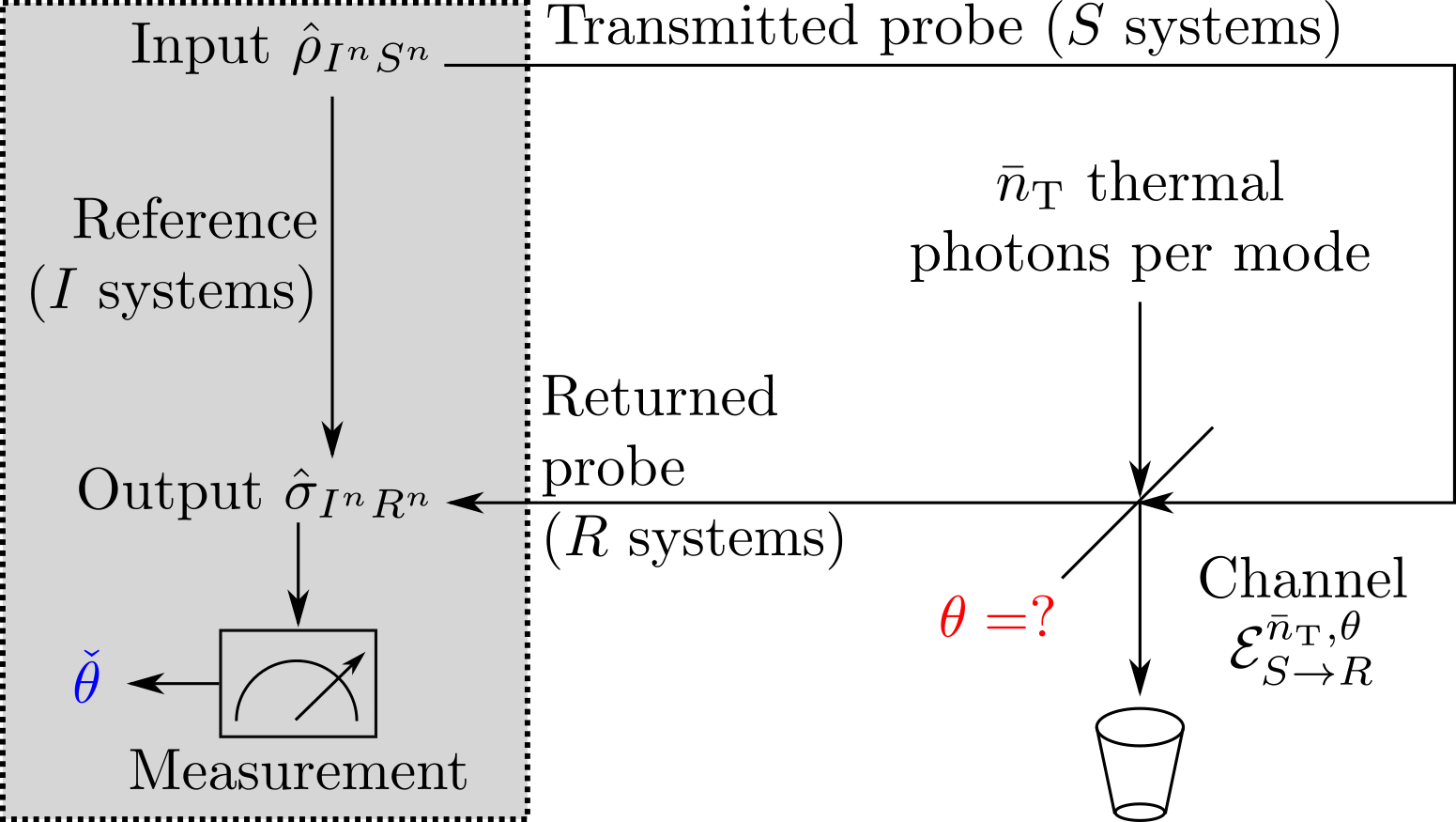
Figure 1: Sensing of unknown transmittance $\theta$; reprint of [12, Fig. 2]. Sensor transmits $n$-mode probes (systems $S$ of bipartite state $\hat{\rho}_{I^{n}S^{n}}$) into a thermal noise lossy bosonic channel $\mathcal{E}^{(\bar{n}_{\rm T},\theta)}$ modeled by a beamsplitter with unknown transmittance $\theta$ mixing signal and a thermal state with mean thermal photon number $\bar{n}_{\rm T}\equiv\frac{\bar{n}_{\rm B}}{1-\theta}$. Reference idler systems $I$ are used in the measurement of output state $\hat{\sigma}_{I^{n}R^{n}}(\theta)$, with outcomes passed to estimator $\check{\theta}$.

In [12] we explored quantum-enhanced sensing of unknown power transmittance $\theta$, a problem of great practical importance. Fig. 1 depicts our system model, which uses thermal noise lossy bosonic channel $\mathcal{E}^{(\bar{n}_{\rm T},\theta)}$, a quantum-mechanical description of many practical channels including optical, microwave, and radio-frequency. To prevent the noise from carrying useful information about $\theta$ to the sensor (so-called “shadow effect” [16]), we set the thermal environment mean photon number $\bar{n}_{\rm T}\equiv\frac{\bar{n}_{\rm B}}{1-\theta}$, as in the literature [17, 18, 19, 20, 21, 22].

The sensor employs a bipartite quantum state $\hat{\rho}_{I^{n}S^{n}}$ containing $n$ signal and idler systems $S$ and $I$. Signal systems $S$ interrogate the target using $n$ available modes of channel $\mathcal{E}^{\bar{n}_{\rm T},\theta}_{S\rightarrow R}$, while the idler systems $I$ are retained losslessly and noiselessly as a reference. A spatio-temporal-polarization mode is a fundamental transmission unit (akin to a channel use) in quantum optics. We showed that the optimal quantum state for transmittance sensing with small mean probe photon number per mode $\bar{n}_{\rm S}\to 0$ is the two-mode squeezed vacuum (TMSV) state (subsequently, it was proved [16] to be an optimal Gaussian quantum state). We also derived the corresponding optimal POVM from the eigen-states of the SLD, per Section II-A: a two-mode squeezer with squeezing parameter $\omega$ followed by the photon-number-resolving (PNR) measurements of each output mode. Fig. 2 in Appendix A diagrams the sensor.

Our measurement consists of well-known optical components. Although this tremendous advantage allows possible use in practice, there are two caveats. First, whether this measurement exists (i.e., whether a solution for $\omega$ can be found) depends on the values of $\theta$, $\bar{n}_{\rm S}$ and $\bar{n}_{\rm B}$, as illustrated in [12, Fig. 4]. Thus, the parameter space that this measurement covers is $\Gamma=[\theta^{\prime\prime},1]$, where $\theta^{\prime\prime}>0$ is a function of $\bar{n}_{\rm S}$ and $\bar{n}_{\rm B}$. Different, possibly suboptimal, measurement must be used outside of this parameter space. Second, the measurement structure determined by $\omega$ depends on the parameter of interest $\theta$. However, this can addressed by a two-stage method introduced in Section II-B.

In the preliminary stage, shown on Fig. 3 in Appendix A, we employ a laser-light (coherent state) probe with mean photon number per mode $\bar{n}_{\rm S}$. We prove that MLE applied to homodyne measurement outcomes is strongly consistent in Appendix B, thus satisfying the strong condition 1 in Theorem 1. We use our optimal measurement in the refinement stage. The statistics of its output are described by an i.i.d. sequence of data pairs corresponding to the photon counts in each PNR detector $\left\{\left(K_{i},M_{i}\right)\right\}_{i=f(n)+1}^{n}$ (although $K_{i}$ and $M_{i}$ in each pair are correlated). The p.m.f. is [12, eq. (35)]:

$$\IEEEeqnarraymulticol{3}{l}{p_{K,M}(k,m;\theta,\check{\theta}_{\rm p})}$$ (32)

$$= \sum_{s=\max(k-m,0)}^{\infty}r_{s,s-k+m}\tau_{0}^{2(s-k)}s!(s-k+m)!k!m!$$

$$\times\bigg{|}\sum_{u=\max(0,k-s)}^{\min(k,m)}\frac{(-\tau_{0}^{2})^{u}\nu_{0}^{-(k+m-2u+1)}}{(s-k+u)!u!(k-u)!(m-u)!}\bigg{|}^{2},$$

where $r_{s,t}=\frac{N_{1}^{s}N_{2}^{t}}{(1+N_{1})^{s+1}(1+N_{2})^{t+1}}$, $N_{1},N_{2},\nu_{0}>1$, and $\tau_{0}\in(0,1)$. We defer the details to [12]. Note that our two stages differ not only in the measurement structure but also in the quantum state being measured. However, the results of Section III apply in such scenarios. Although the MLE of $\theta$ for the optimal receiver has no closed form, we prove its strong consistency and asymptotic normality in Appendices C and D, meeting condition 2 of Theorem 1. Furthermore, the squeezing parameter $\omega$ is continuous in the preliminary estimate $\check{\theta}_{\rm p}$, and the FI associated with $\theta$ in $(K,M)$ is continuous in $\omega$, satisfying condition 3 of Theorem 1.

V Conclusion

Quantum estimation theory yields optimal measurements of a scalar parameter embedded in a quantum state [1]. However, often, these measurements depend on the parameter of interest. This necessitates a two-stage approach [4, 5], [6, Ch. 6.4], where a preliminary estimate is derived from a sub-optimal measurement, and is then used to construct an optimal measurement that yields a refined estimate. Here, we establish the conditions for the strong and weak consistency as well as the asymptotic normality of this two-stage approach, with QCRB being the variance of the limiting Gaussian in the latter claim. This matches the usual asymptotic properties for the MLEs. We then apply our methodology to show that the quantum-enhanced transmittance estimator from [12] is strongly consistent and asymptotically normal.

Although out of scope in this paper, extending our results to multiple parameters is an intriguing area for future work. Attaining multi-parameter QCRB [1, Ch. VIII.4(a)] is complicated by the non-commutativity of quantum measurements for each parameter. A potential direction of research would focus on investigating the asymptotics of quantum estimators in the context of Holevo-Cramér-Rao [23] and quasi-Cramér-Rao [13, 14] bounds. In the immediate term, our results will allow establishing optimality claims for various single-parameter quantum estimation problems. Indeed, we will apply them to robust quantum-inspired super-resolution imaging [24].

Appendix A Transmittance Sensor Diagrams

Fig. 2 diagrams the sensor that employs TMSV and an optimal POVM that is described in Section IV and in [12]. This sensor is used in the refinement stage of transmittance sensing. Fig. 3 shows the coherent sensor used in the preliminary stage.

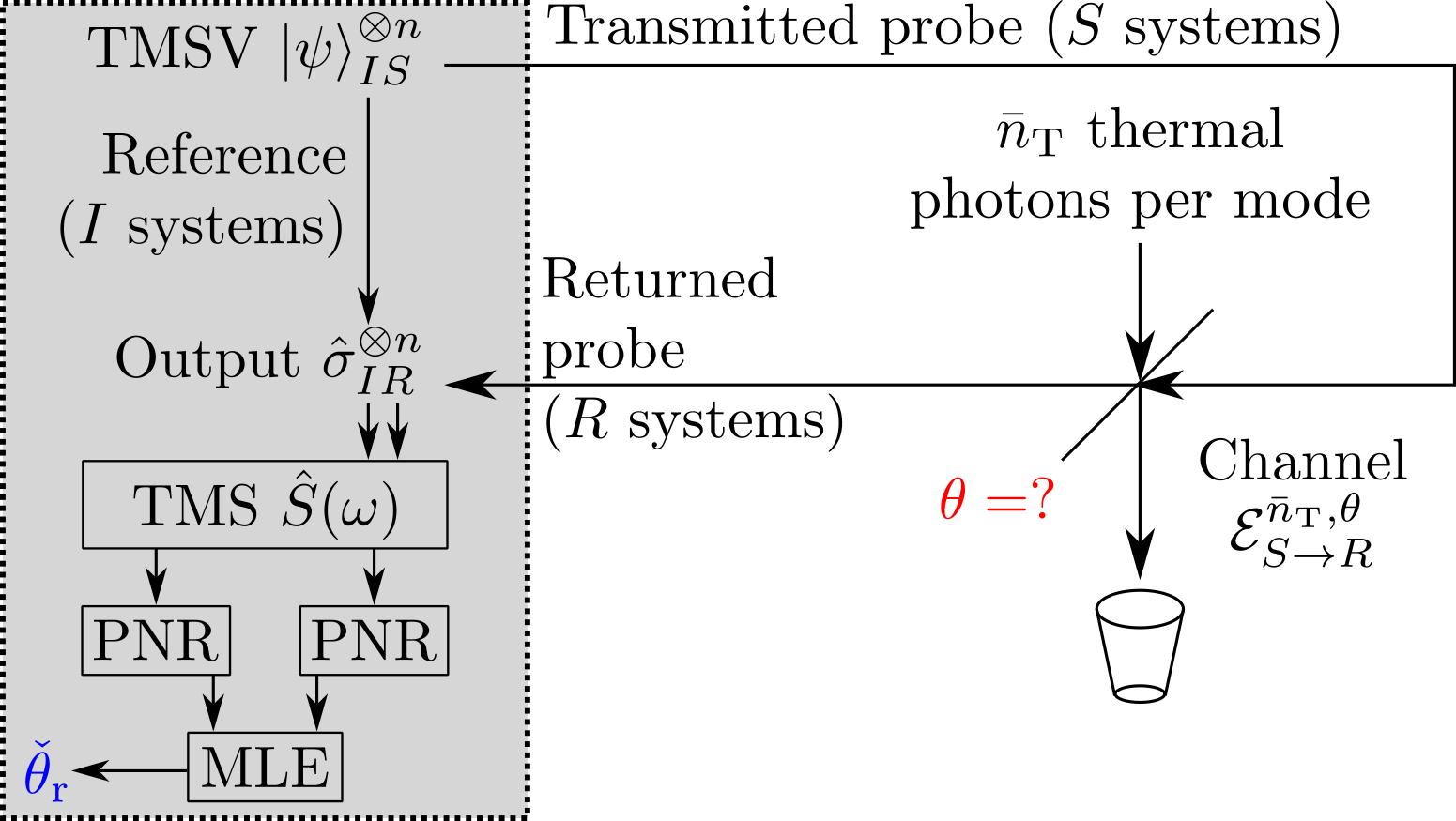
Figure 2: Sensing the unknown transmittance $\theta$ using $n$ two-mode squeezed vacuum (TMSV) states $\left|\psi\right>_{IS}$; reprint of [12, Fig. 3]. When $\left|\psi\right>_{IS}$ is transmitted, a bipartite output state $\hat{\sigma}_{IR}$ occupies a retained idler system $I$ and a corresponding returned probe system $R$. The receiver achieves QCRB by applying a two-mode squeezer (TMS) separately to each of the $n$ output states $\hat{\sigma}_{IR}$, followed by independent photon-number-resolving (PNR) measurement of each output mode. MLE is used on the resulting classical output to obtain the estimate $\check{\theta}_{\rm r}$. As in Fig. 1, $\bar{n}_{\rm T}\equiv\frac{\bar{n}_{\rm B}}{1-\theta}$.

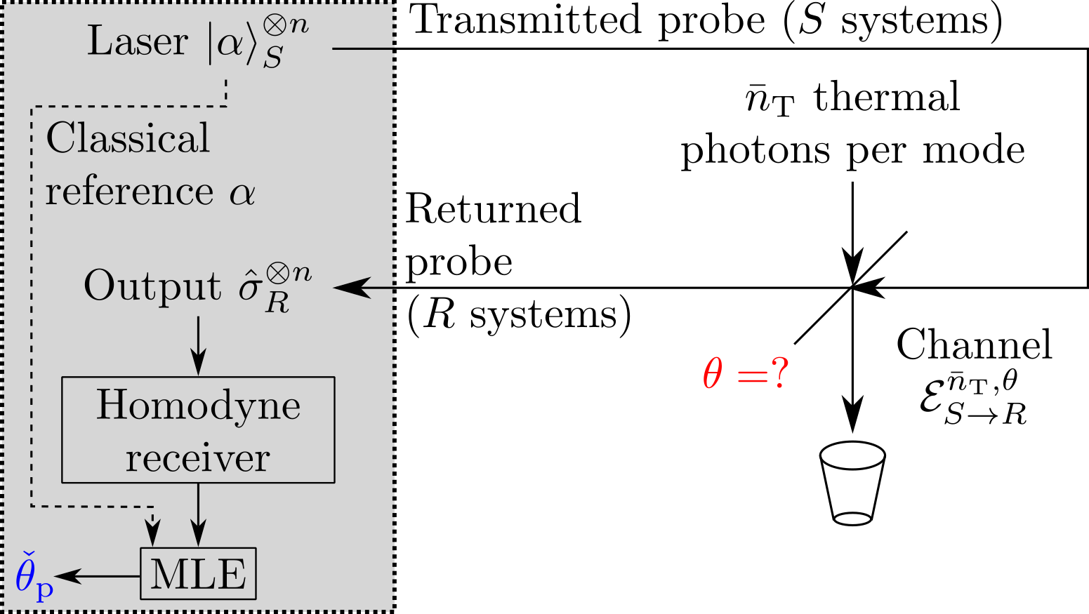
Figure 3: Sensing the unknown transmittance $\theta$ using $n$ coherent states $\left|\alpha\right>_{S}$ and a homodyne measurement. The output state $\hat{\sigma}_{R}$ is a displaced thermal state. A Gaussian random variable describes the output of homodyne measurement [25],[26, Ch. 7.3.2]. An MLE $\check{\theta}_{\rm p}$ that uses the homodyne receiver’s output and the value of $\alpha$ as a classical reference is analyzed in Appendix B.

Appendix B Consistency of the Preliminary Transmittance Estimator

Consider the coherent sensor in Fig. 3. The homodyne measurement on the returned states outputs a sequence of $f(n)$ i.i.d. Gaussian random variables $\left\{X_{i}\right\}_{i=1}^{f(n)}$, where $X_{1}\sim\mathcal{N}\left(\sqrt{\theta\bar{n}_{\rm S}},\bar{n}_{\rm B}+1\right)$ [12, Sec. V-A and VI-A.1]. The MLE for $\theta$ is: $\check{\theta}_{\rm p}=\frac{1}{\bar{n}_{\rm S}}\left(\frac{1}{f(n)}\sum_{i=1}^{f(n)}x_{i}\right)^{2}$, where $x_{i}$ is an observed instance of $X_{i}$. The estimator $\check{\Theta}_{\rm p}=\left(\frac{1}{f(n)\sqrt{\bar{n}_{\rm S}}}\sum_{i=1}^{f(n)}X_{i}\right)^{2}=Z^{2}$, $X_{i}\sim\mathcal{N}\left(\sqrt{\theta\bar{n}_{\rm S}},\frac{\bar{n}_{\rm B}+1}{2}\right)$ and $Z\sim\mathcal{N}\left(\sqrt{\theta},\sigma^{2}\right)$, where $\sigma^{2}=\frac{\bar{n}_{\rm B}+1}{2f(n)\bar{n}_{\rm S}}$ and $f(n)\in\omega(1)\cap o(n)$ is the number of modes used for sensing in the preliminary stage. We first show weak consistency of $\check{\theta}_{\rm p}$ using the standard methods, and then strengthen these to yield strong consistency. We have

$$\IEEEeqnarraymulticol{3}{l}{\Pr\{|\check{\Theta}_{\rm p}-\theta_{0}|>\epsilon_{4}\}}$$

$$= \Pr\left\{\check{\Theta}_{\rm p}\in[0,\theta_{0}-\epsilon_{4})\cup(\theta_{0}+\epsilon_{4},\infty)\right\}$$

$$= \Pr\Big{\{}Z\in(-\infty,-\sqrt{\theta_{0}+\epsilon_{4}})$$

$$\phantom{\lim\limits_{n\to\infty}\sqrt{n}}\cup(-\sqrt{\theta_{0}-\epsilon_{4}},\sqrt{\theta_{0}-\epsilon_{4}})\cup(\sqrt{\theta_{0}+\epsilon_{4}},\infty)\Big{\}}$$

$$\IEEEeqnarraymulticol{3}{l}{\leq\Pr\left\{Z\in(-\infty,\sqrt{\theta_{0}-\epsilon_{4}})\cup(\sqrt{\theta_{0}+\epsilon_{4}},\infty)\right\}}$$ (33)

$$= \operatorname{erfc}\left(\frac{\sqrt{\theta_{0}+\epsilon_{4}}-\sqrt{\theta_{0}}}{\sqrt{2}\sigma}\right)+\operatorname{erfc}\left(\frac{\sqrt{\theta_{0}}-\sqrt{\theta_{0}-\epsilon_{4}}}{\sqrt{2}\sigma}\right)$$

$$\leq e^{-b_{1}f(n)}+e^{-b_{2}f(n)},$$

where $b_{1}=\frac{\bar{n}_{\rm S}^{2}(\sqrt{\theta_{0}+\epsilon_{4}}-\sqrt{\theta_{0}})^{2}}{\bar{n}_{\rm B}+1}$ and $b_{2}=\frac{\bar{n}_{\rm S}^{2}(\sqrt{\theta_{0}}-\sqrt{\theta_{0}-\epsilon_{4}})^{2}}{\bar{n}_{\rm B}+1}$, $\operatorname{erfc}(x)$ is the Gaussian error function:

$$\text{efrc}(x)=\frac{2}{\sqrt{\pi}}\int_{x}^{\infty}e^{-t^{2}}dt,$$ (34)

and (33) is by the Chernoff bound for the error function [27]. Weak consistency $\check{\Theta}_{\rm p}\xrightarrow{p}\theta_{0}$ follows from taking the limit of (33) as $n\to\infty$.

To obtain strong consistency, we recall that $\check{\Theta}_{\rm p}$ functionally depends on $n$ through $f(n)$ and define a set $A_{y}=\left\{\check{\Theta}_{\rm p}:\left|\check{\Theta}_{\rm p}-\theta_{0}\right|\geq\epsilon_{4},f(n)\in[2^{y-1},2^{y})\right\}$. We have

$$\IEEEeqnarraymulticol{3}{l}{\Pr(A_{y})\leq\sum_{f(n)=2^{y-1}}^{2^{y}-1}(e^{-b_{1}f(n)}+e^{-b_{2}f(n)})}$$ (35)

$$= \frac{e^{-2^{y}b_{1}}(-e^{b_{1}}+e^{2^{-1+y}b_{1}})}{b_{1}}+\frac{e^{-2^{y}b_{2}}(-e^{b_{2}}+e^{2^{-1+y}b_{2}})}{b_{2}}$$

$$= c_{y}+d_{y}.$$

Since $\lim\limits_{y\to\infty}\left|\frac{c_{y+1}}{c_{y}}\right|=0$, $\lim\limits_{y\to\infty}\left|\frac{d_{y+1}}{d_{y}}\right|=0$ by the ratio test [28, Ch. 23, Th. 3],

$$\sum_{y=1}^{\infty}\Pr(A_{y})=\sum_{y=1}^{\infty}c_{y}+\sum_{y=1}^{\infty}d_{y}<\infty.$$ (36)

Thus, by Borel-Cantelli theorem [29, Th. 10.10],

$$\Pr\left\{\limsup_{y\to\infty}A_{y}\right\}=0,$$ (37)

where $\limsup_{y\to\infty}A_{y}$ is the set of $\check{\Theta}_{\rm p}$ such that $\left|\check{\Theta}_{\rm p}-\theta_{0}\right|\geq\epsilon_{4}$ for infinitely many values of $f(n)$. Since $f(n)\in\omega(1)$,

$$\Pr\left\{\limsup_{n\to\infty}\left|\check{\Theta}_{\rm p}-\theta_{0}\right|<\epsilon_{4}\right\}=1,$$ (38)

and we obtain strong consistency $\check{\Theta}_{\rm p}\xrightarrow{a.s.}\theta_{0}$.

Appendix C Consistency of MLE Applied to Optimal Transmittance Measurement Outcomes

The expectations here are with respect to $(K,M)$, thus, we drop the subscript $KM$ from $E_{KM}[\cdot]$ for brevity. Per Section IV, $\Gamma\equiv[\theta^{\prime\prime},1]$. First, we introduce separability:

Definition 1 (Separability [30, Assumption A-1]).

For every $\theta\in\Gamma$, a measurable function $f(a,\theta)$ is separable if there is a null set $\mathcal{U}$ and a countable subset $\Gamma^{\prime}\subset\Gamma$ such that for every open set $\mathcal{T}\subset\Gamma$ and every closed interval $B$, the sets $\left\{x|f(a,\theta)\in B,\forall\theta\in\mathcal{T}\right\}$ and $\left\{x|f(a,\theta)\in B,\forall\theta\in\mathcal{T}\cap\Gamma^{\prime}\right\}$ differ by at most a subset of $\mathcal{U}$.

Note that $f(a;\theta)$ is separable if it is continuous for each $\theta$ [15, Ex. 38.3]. Now we adapt the conditions for strong consistency of MLE in [31, Th. 1],

Lemma 2.

Let $\{A_{i}\}_{i=1}^{n}$ be a sequence of i.i.d. random variables describing the observations, each with p.d.f. $p\left(a_{i};\theta_{0}\right)$. Let $\check{\Theta}$ statistically describe an MLE for $\theta$. Then $\check{\Theta}\xrightarrow{a.s.}\theta_{0}$, if

1. $\log p\left(a;\theta\right)$ has a unique maximum for each $a$;

2. $\log p\left(a;\theta\right)$ is measurable in $a$ for all $\theta$;

3. $\log p\left(a;\theta\right)$ is separable per Definition 1;

4. $\log p\left(A_{i};\theta\right)$ is continuous almost everywhere: for all $\theta$, $\Pr\left(\left\{a:\lim_{\gamma\to\theta}p(a,\gamma)=p(a,\theta)\right\}\right)=1$;

5. $\left|\log p\left(A_{i};\theta\right)\right|\leq g\left(A_{i}\right)$, where $E_{A_{i}}\left[g\left(A_{i}\right)\right]<\infty$.

Now we employ Lemma 2 to show strong consistency of the MLE applied to the output of our optimal (SLD-based) transmittance measurement. Conditions 1-4 are satisfied by inspection: $p(k,m;\theta,\check{\theta}_{\rm p})$ has a unique maximum per [10, Lemma 2.2] as $p(k,m;\theta_{1},\check{\theta}_{\rm p})\neq p(k,m;\theta_{2},\check{\theta}_{\rm p})$ when $\theta_{1}\neq\theta_{2}$, $p(k,m;\theta,\check{\theta}_{\rm p})$ is measurable since it is a continuous function on the counting measure, and $p(k,m;\theta,\check{\theta}_{\rm p})$ is continuous for each $\theta\in\Gamma$, implying that it is also separable [15, Ex. 38.3]. To verify condition 5, we define the dominating function $\sup_{\theta\in\Gamma}\left|\log(p(K,M;\theta,\check{\theta}_{\rm p}))\right|$, and show that:

$$\IEEEeqnarraymulticol{3}{l}{E\left[\sup_{\theta\in\Gamma}\left|\log(p(K,M;\theta,\check{\theta}_{\rm p}))\right|\right]<\infty}.$$ (39)

We upper-bound $\left|\log\left(p(k,m;\theta,\check{\theta}_{\rm p}\right)\right|$ by lower-bounding $p\left(k,m;\theta,\check{\theta}_{\rm p}\right)$, as it is in $(0,1]$. Since each term in the summation over $s$ defining $p\left(k,m;\theta,\check{\theta}_{\rm p}\right)$ in (32) is non-negative, any of them yield a lower bound. When $k\leq m$, we let $s=0$:

$$p(k,m;\theta,\check{\theta}_{\rm p}) \geq r_{0,m-k}(\tau_{0})^{-2k}(m-k)!k!m!$$ (40)

$$\times\bigg{|}\sum_{u=k}^{k}\frac{(-\tau_{0}^{2})^{u}\nu_{0}^{-(k+m-2u+1)}}{(-k+u)!u!(k-u)!(m-u)!}\bigg{|}^{2}$$

$$= r_{0,m-k}\tau_{0}^{2k}\frac{m!}{k!(m-k)!}\nu_{0}^{-2(m-k+1)}$$

$$\geq r_{0,m-k}\tau_{0}^{2k}\nu_{0}^{-2(m-k+1)}.$$

When $k\geq m$, we let $s=k-m$:

$$\IEEEeqnarraymulticol{3}{l}{p(k,m;\theta,\check{\theta}_{\rm p})\geq r_{k-m,0}\tau_{0}^{2m}\nu_{0}^{-2(k-m+1)}.}$$ (41)

Since $0\leq\tau_{0}<1$ and $\nu_{0}>1$, for all $k$ and $m$, we have

$$p(k,m;\theta,\check{\theta}_{\rm p})\geq r_{k,m}\tau_{0}^{2\min(k,m)}\nu_{0}^{-2(k+m+1)}.$$ (42)

Let $\nu_{0}^{\ast}=\inf_{\theta\in\Gamma}\nu_{0}$ and $\tau_{0}^{\ast}=\inf_{\theta\in\Gamma}\tau_{0}$. Furthermore, let $L_{\rm{n},1}^{\ast}=\sup_{\theta\in\Gamma}\log(1/N_{1})$ $L_{\rm{d},1}^{\ast}=\sup_{\theta\in\Gamma}\log(N_{1}+1)$, and, similarly, $L_{\rm{n},2}^{\ast}=\sup_{\theta\in\Gamma}\log(1/N_{2})$ $L_{\rm{d},2}^{\ast}=\sup_{\theta\in\Gamma}\log(N_{2}+1)$. Since $0<p(k,m;\theta,\check{\theta}_{\rm p})<1$,

$$\IEEEeqnarraymulticol{3}{l}{E\left[\sup_{\theta\in\Gamma}\left|\log(p(K,M;\theta,\check{\theta}_{\rm p}))\right|\right]}$$ (43)

$$\leq -E\left[\log r_{K,M}\right]-E\left[\log\tau_{0}^{\ast 2\min(K,M)}\right]$$

$$-E\left[-2(K+M+1)\log\nu_{0}^{\ast}\right]$$

$$\leq \left(E\left[K\right]+1\right)L_{\rm{d},1}^{\ast}+E\left[K\right]L_{\rm{n},1}^{\ast}$$

$$+\left(E\left[M\right]+1\right)L_{\rm{d},2}^{\ast}+E\left[M\right]L_{\rm{n},2}^{\ast}$$

$$-2E\left[(\min(K,M))\right]\log\tau_{0}^{\ast}$$

$$+2E\left[(K+M+1)\right]\log\nu_{0}^{\ast}.$$

Since the energy of the received photons is finite, $E[K]$ and $E[M]$ are finite for all $\theta$. Furthermore, $E\left[(\min(K,M))\right]\leq\min\left(E[K],E[M]\right)$. Thus, every term in (43) is finite, satisfying (39) and resulting in strong consistency: $\check{\Theta}_{\rm r}\left(\check{\theta}_{\rm p}\right)\xrightarrow{a.s.}\theta_{0}$.

Appendix D Asymptotic Normality of MLE Applied to Optimal Transmittance Measurement Outcomes

Again, the expectations here are with respect to $(K,M)$, and we drop the subscript $KM$ from $E_{KM}[\cdot]$. Let $n^{\prime}\equiv n-f(n)$. First, for $\theta\in\Gamma\equiv[\theta^{\prime\prime},1]$, these regularity conditions hold:

$$\sum_{km}\partial_{\theta}p(k,m;\theta,\check{\theta}_{\rm p}) =\partial_{\theta}\sum_{km}p(k,m;\theta,\check{\theta}_{\rm p})=0$$ (44)

$$\sum_{km}\partial^{2}_{\theta}p(k,m;\theta,\check{\theta}_{\rm p}) =\partial^{2}_{\theta}\sum_{km}p(k,m;\theta,\check{\theta}_{\rm p})=0.$$ (45)

The proof is in Appendix E. Furthermore, $\partial_{\theta}p(k,m;\theta,\check{\theta}_{\rm p})$ and $\partial^{2}_{\theta}p(k,m;\theta,\check{\theta}_{\rm p})$ exist and are continuous for all $\theta,\check{\theta}_{\rm p}\in\left[\theta^{\prime\prime},1\right]$. By [9, Prop. IV.C.4], (44) and (45) yield:

$$\mathcal{I}_{\theta_{0},\check{\theta}_{p}} =E\left[\left(\partial_{\theta}\log p(K,M;\theta,\check{\theta}_{p})\right)^{2}\Big{|}_{\theta=\theta_{0}}\right]$$

$$=-E\left[\left(\partial^{2}_{\theta}\log p(K,M;\theta,\check{\theta}_{p})\right)\Big{|}_{\theta=\theta_{0}}\right].$$ (46)

By the definition of the MLE, we select $\check{\Theta}_{\rm r}\left(\check{\theta}_{\rm p}\right)$ such that

$$\frac{1}{n^{\prime}}\sum_{i}\partial_{\theta}\log p(K_{i},M_{i};\theta,\check{\theta}_{\rm p})\Big{|}_{\theta=\check{\Theta}_{\rm r}\left(\check{\theta}_{\rm p}\right)}=0,$$ (47)

where the summations over $i$ here are from $i=f(n)+1$ to $i=n$. Application of the mean value theorem to (47) yields:

$$\sqrt{n^{\prime}}\left(\check{\Theta}_{\rm r}\left(\check{\theta}_{\rm p}\right)-\theta_{0}\right)\\ =\frac{\frac{1}{\sqrt{n^{\prime}}}\sum_{i}\left(\partial_{\theta}\log p\left(K_{i},M_{i};\theta,\check{\theta}_{\rm p}\right)\right)\Big{|}_{\theta=\theta_{0}}}{-\frac{1}{n^{\prime}}\sum_{i}\left(\partial^{2}_{\theta}\log p\left(K_{i},M_{i};\theta,\check{\theta}_{\rm p}\right)\right)\Big{|}_{\theta=\bar{\Theta}}},$$ (48)

where $\left|\bar{\Theta}-\theta_{0}\right|\leq\left|\check{\Theta}_{\rm r}\left(\check{\theta}_{\rm p}\right)-\theta_{0}\right|$. Consistency of $\check{\Theta}_{\rm r}\left(\check{\theta}_{\rm p}\right)$ shown in Appendix C yields:

$$\bar{\Theta}\overset{p}{\to}\theta_{0}.$$ (49)

Now we adapt the standard results (e.g., from [9, Prop. IV.D.2]). Consider the numerator in (48). By (44), we have $E\left[\left(\partial_{\theta}\log p\left(K,M;\theta,\check{\theta}_{\rm p}\right)\right)\Big{|}_{\theta=\theta_{0}}\right]=0$. As the FI is bounded, the variance of $\partial_{\theta}\log p\left(K,M;\theta,\check{\theta}_{\rm p}\right)\Big{|}_{\theta=\theta_{0}}$ is: $E\left[\left(\partial_{\theta}\log p\left(K,M;\theta,\check{\theta}_{\rm p}\right)\right)^{2}\Big{|}_{\theta=\theta_{0}}\right]=\mathcal{I}_{\theta_{0},\check{\theta}_{\rm p}}<\infty$. By the central limit theorem,

$$\frac{1}{\sqrt{n^{\prime}}}\sum_{i}\partial_{\theta}\log p\left(K,M;\theta,\check{\theta}_{\rm p}\right)\Big{|}_{\theta=\theta_{0}}\overset{d}{\to}\mathcal{N}\left(0,\mathcal{I}_{\theta_{0},\check{\theta}_{\rm p}}\right).$$ (50)

Consider the denominator in (48). By the weak law of large numbers (WLLN),

$$\frac{1}{n^{\prime}}\sum_{i}\partial^{2}_{\theta}\log p\left(K_{i},M_{i};\theta,\check{\theta}_{\rm p}\right)\Big{|}_{\theta=\theta_{0}}\overset{p}{\to}\mathcal{I}_{\theta_{0},\check{\theta}_{\rm p}}.$$ (51)

Thus, for $\epsilon_{5}>0$,

$$\IEEEeqnarraymulticol{3}{l}{\Pr\left\{\left|\frac{1}{n^{\prime}}\sum_{i}\partial^{2}_{\theta}\log p\left(K_{i},M_{i};\theta,\check{\theta}_{\rm p}\right)\Big{|}_{\theta=\bar{\Theta}}-\mathcal{I}_{\theta_{0},\check{\theta}_{\rm p}}\right|>\epsilon_{5}\right\}}$$ (53)

$$= \Pr\bigg{\{}\bigg{|}\frac{1}{n^{\prime}}\sum_{i}\partial^{2}_{\theta}\log p\left(K_{i},M_{i};\theta,\check{\theta}_{\rm p}\right)\Big{|}_{\theta=\bar{\Theta}}-\mathcal{I}_{\theta_{0},\check{\theta}_{\rm p}}$$

$$-\frac{1}{n^{\prime}}\sum_{i}\partial^{2}_{\theta}\log p\left(K_{i},M_{i};\theta,\check{\theta}_{\rm p}\right)\Big{|}_{\theta=\theta_{0}}$$

$$+\frac{1}{n^{\prime}}\sum_{i}\partial^{2}_{\theta}\log p\left(K_{i},M_{i};\theta,\check{\theta}_{\rm p}\right)\Big{|}_{\theta=\theta_{0}}\bigg{|}>\epsilon_{5}\bigg{\}}$$

$$\leq \Pr\bigg{\{}\bigg{|}\frac{1}{n^{\prime}}\sum_{i}\partial^{2}_{\theta}\log p\left(K_{i},M_{i};\theta,\check{\theta}_{\rm p}\right)\Big{|}_{\theta=\bar{\Theta}}$$

$$-\frac{1}{n^{\prime}}\sum_{i}\partial^{2}_{\theta}\log p\left(K_{i},M_{i};\theta,\check{\theta}_{\rm p}\right)\Big{|}_{\theta=\theta_{0}}\bigg{|}>\frac{\epsilon_{5}}{2}\bigg{\}}$$

$$+\Pr\left\{\bigg{|}\frac{1}{n^{\prime}}\sum_{i}\partial^{2}_{\theta}\log p\left(K_{i},M_{i};\theta,\check{\theta}_{\rm p}\right)\Big{|}_{\theta=\theta_{0}}\right.$$

$$\phantom{\frac{1}{n^{\prime}}\sum_{i}\partial^{2}_{\theta}\log p\left(K_{i},M_{i};\theta,\check{\theta}_{\rm p}\right)}\quad\left.-\mathcal{I}_{\theta_{0},\check{\theta}_{\rm p}}\bigg{|}>\frac{\epsilon_{5}}{2}\right\}.$$

The first term in (53) is zero by the continuity of $\frac{1}{n^{\prime}}\sum_{i}\partial^{2}_{\theta}\log p(k_{i},m_{i};\theta,\check{\theta}_{\rm p})$ over $\theta$, (49), and continuous mapping theorem [15, Th. 25.7]. The second term in (53) is zero by $\eqref{eq:d weak}$. Therefore,

$$\frac{1}{n^{\prime}}\sum_{i}\partial^{2}_{\theta}\log p(K_{i},M_{i};\theta,\check{\theta}_{\rm p})\Big{|}_{\theta=\bar{\Theta}}\overset{p}{\to}\mathcal{I}_{\theta_{0},\check{\theta}_{\rm p}}.$$ (54)

Combining (50) and (54) using Slutsky’s theorem yields

$$\sqrt{n^{\prime}}\left(\check{\Theta}_{\rm r}\left(\check{\theta}_{\rm p}\right)-\theta_{0}\right)\overset{d}{\to}\mathcal{N}\left(0,\mathcal{I}_{\theta_{0},\check{\theta}_{\rm p}}^{-1}\right).$$ (55)

Therefore, all the conditions of Theorem 1 are met and the overall two-stage transmittance estimator is strongly consistent and asymptotically normal.

Appendix E Regularity Conditions for Asymptotic Normality

First, we state a useful lemma [32, Th. 3]:

Lemma 3.

Let $X$ be an open subset of $\mathbb{R}$, and $Y$ be a measure space. Suppose $f:X\times Y\to\mathbb{R}$ satisfies the following conditions

1. f(x,y) is a measurable function of $x$ and $y$ jointly, and is integrable over $y$, for almost all $x\in X$.

2. For almost all $y\in Y$, $f(x,y)$ is an absolutely continuous function (see definition in [29, Eq. (3.31)]) of $x$.

3. For all compact intervals $[a,b]\subseteq X$:

   $$\int_{a}^{b}\int_{Y}\left|\partial_{x}f(x,y)\right|dydx<\infty.$$ (56)

Then, $\int_{Y}f(x,y)dy$ is an absolutely continuous function of $x$, and, for almost all $x\in X$, its derivative exists and is:

$$\partial_{x}\int_{Y}f(x,y)dy=\int_{Y}\partial_{x}f(x,y)dy.$$ (57)

Although Lemma 3 is stated as [32, Th. 3], we could not find its proof in the literature. Thus, we provide the adaptation of [33, Th. 4] for completeness:

Proof (Lemma 3).

For almost all $x\in X$ and $y\in Y$,

$$\IEEEeqnarraymulticol{3}{l}{\partial_{x}\int_{Y}f(x,y)dy=\lim\limits_{h\to 0}\frac{1}{h}\left[\int_{Y}f(x+h,y)-f(x,y)dy\right]}$$ (61)

$$\phantom{\lim\limits_{h\to 0}\frac{1}{h}}=\lim\limits_{h\to 0}\frac{1}{h}\left[\int_{Y}\int_{x}^{x+h}\partial_{x}f(x,y)dxdy\right]$$

$$\phantom{\lim\limits_{h\to 0}\frac{1}{h}}=\lim\limits_{h\to 0}\frac{1}{h}\left[\int_{x}^{x+h}\int_{Y}\partial_{x}f(x,y)dydx\right]$$

$$\phantom{\lim\limits_{h\to 0}\frac{1}{h}}=\int_{Y}\partial_{x}f(x,y)dy,$$

where (61) is by the definition of derivative, (61) is by condition 2 and the fundamental theorem of calculus for Lebesgue integral (FTCL) [29, Th. 3.35], and (61) is by condition 3, and Fubini’s and Tonelli’s theorems. Furthermore, (61) shows that $\int_{Y}f(b,y)dy-\int_{Y}f(a,y)dy=\int_{a}^{b}\int_{Y}\partial_{x}f(x,y)dydx$. Thus, $\int_{Y}f(x,y)dy$ is an absolutely continuous function for almost all $x\in X$ by condition 3 and FTCL. ∎

We show (44) and (45) by using Lemma 3 on $p(k,m;\theta,\check{\theta}_{p})$, with $X$ being $\Gamma$, and $Y$ being the space of $K\times M$, that is, a product counting measure space. Condition 1 of Lemma 3 holds since $p(k,m;\theta,\check{\theta}_{p})$ and $\partial_{\theta}p(k,m;\theta,\check{\theta}_{p})$ are continuous over $\theta$ and, hence, measurable [29, Cor. 2.2]. For condition 2, we first show integrability: $\sum_{km}|p(k,m;\theta,\check{\theta}_{p})|=1$ since $p(k,m;\theta,\check{\theta}_{p})$ is a p.d.f. and $\sum_{km}|\partial_{\theta}p(k,m;\theta,\check{\theta}_{p})|<\infty$ by (87). Then, for all compact intervals $[\theta_{1},\theta_{2}]\subseteq\Gamma$, $p(k,m;\theta,\check{\theta}_{p})$ and $\partial_{\theta}p(k,m;\theta,\check{\theta}_{p})$ are absolutely continuous by FTCL since

$$p(k,m;\theta_{2},\check{\theta}_{p})-p(k,m;\theta_{1},\check{\theta}_{p})\\ =\int_{\theta_{1}}^{\theta_{2}}\partial_{\theta}p(k,m;\theta,\check{\theta}_{p})d\theta,$$

$$\partial_{\theta}p(k,m;\theta_{2},\check{\theta}_{p})-\partial_{\theta}p(k,m;\theta_{1},\check{\theta}_{p})\\ =\int_{\theta_{1}}^{\theta_{2}}\partial^{2}_{\theta}p(k,m;\theta,\check{\theta}_{p})d\theta,$$

and $\partial_{\theta}p(k,m;\theta,\check{\theta}_{p})$ and $\partial^{2}_{\theta}p(k,m;\theta,\check{\theta}_{p})$ are integrable by (87) and (88). For any $[\theta_{1},\theta_{2}]\subseteq\Gamma\equiv\left[\theta^{\prime\prime},1\right]$, we need:

$$\IEEEeqnarraymulticol{3}{l}{\int_{\theta_{1}}^{\theta_{2}}\sum_{km}\left|\partial_{\theta}p(k,m;\theta,\check{\theta}_{\rm p})\right|d\theta\leq\int_{\theta^{\prime\prime}}^{1}\sum_{km}\left|\partial_{\theta}p(k,m;\theta,\check{\theta}_{\rm p})\right|d\theta}$$ (62)

$$\phantom{\sum_{km}\partial_{\theta}}\leq\max_{\theta\in\Gamma}\sum_{km}\left|\partial_{\theta}p(k,m;\theta,\check{\theta}_{\rm p})\right|<\infty$$

$$\IEEEeqnarraymulticol{3}{l}{\int_{\theta_{1}}^{\theta_{2}}\sum_{km}\left|\partial^{2}_{\theta}p(k,m;\theta,\check{\theta}_{\rm p})\right|d\theta\leq\int_{\theta^{\prime\prime}}^{1}\sum_{km}\left|\partial^{2}_{\theta}p(k,m;\theta,\check{\theta}_{\rm p})\right|d\theta}$$ (63)

$$\phantom{\sum_{km}\partial_{\theta}}\leq\max_{\theta\in\Gamma}\sum_{km}\left|\partial^{2}_{\theta}p(k,m;\theta,\check{\theta}_{\rm p})\right|<\infty$$

By [12, App. II.A], $\hat{\sigma}_{\rm IR}=\hat{S}(\zeta)\hat{\sigma}_{IR}^{d}\hat{S}^{\dagger}(\zeta)$ is a two-mode squeezed thermal state, where $\hat{\sigma}_{\rm IR}^{d}=\sum_{km}r_{km}\left|km\right>\left<km\right|$ and $r_{km}$ is defined below (32). Thus, we have:

$$\hat{\sigma}_{IR}^{-1} =\hat{S}(\zeta)\left(\hat{\sigma}_{IR}^{d}\right)^{-1}\hat{S}^{\dagger}(\zeta)$$ (64)

$$\hat{\sigma}_{IR}^{\frac{1}{2}} =\hat{S}(\zeta)\left(\hat{\sigma}_{IR}^{d}\right)^{\frac{1}{2}}\hat{S}^{\dagger}(\zeta).$$ (65)

We use the following traces of the combinations of $\hat{\sigma}_{IR}$ with creation and annihilation operators:

$$\operatorname{Tr}\left\{\hat{\sigma}_{IR}\hat{a}_{R}^{\dagger}\hat{a}_{R}\right\} =\mu^{2}N_{1}+\nu^{2}(1+N_{2})$$ (66)

$$\operatorname{Tr}\left\{\hat{\sigma}_{IR}\hat{a}_{R}\hat{a}_{R}^{\dagger}\right\} =\mu^{2}N_{1}+\nu^{2}(1+N_{2})+1$$ (67)

$$\operatorname{Tr}\left\{\hat{\sigma}_{IR}\hat{a}_{R}^{\dagger}\hat{a}_{R}^{\dagger}\right\} =0$$ (68)

$$\operatorname{Tr}\left\{\hat{\sigma}_{IR}\hat{a}_{R}\hat{a}_{R}\right\} =0$$ (69)

$$\operatorname{Tr}\left\{\hat{\sigma}_{IR}\hat{a}_{R}\hat{a}_{R}^{\dagger}\hat{a}_{R}\hat{a}_{R}^{\dagger}\right\} =1+3N_{1}\mu^{2}+3(1+N_{2})\nu^{2}$$

$$\phantom{=}+2(N_{1}\mu^{2}+(1+N_{2})\nu^{2})^{2}$$ (70)

$$\operatorname{Tr}\left\{\hat{\sigma}_{IR}\hat{a}_{R}^{\dagger}\hat{a}_{R}\hat{a}_{R}^{\dagger}\hat{a}_{R}\right\} =N_{1}\mu^{2}+(1+N_{2})\nu^{2}$$

$$\phantom{=}+2(N_{1}\mu^{2}+(1+N_{2})\nu^{2})^{2}.$$ (71)

Expressions (66)-(71) can be obtained from the fact that $\hat{\sigma}_{IR}$ is Gaussian. The photon probe state evolving in thermal bath is characterized by the Lindblad master equation:

$$\partial_{\theta}\hat{\sigma}_{IR}=-\frac{1}{2\theta}\left[(\bar{n}_{\rm B}+1)\hat{\mathcal{L}}_{R}[\hat{a}]+\bar{n}_{\rm B}\hat{\mathcal{L}}_{R}[\hat{a}^{\dagger}]\right]\hat{\sigma}_{IR},$$ (72)

where

$$\hat{\mathcal{L}}_{R}[\hat{a}]\hat{\sigma}_{IR}=2\hat{a}_{R}\hat{\sigma}_{IR}\hat{a}_{R}^{\dagger}-\hat{a}_{R}^{\dagger}\hat{a}_{R}\hat{\sigma}_{IR}-\hat{\sigma}_{IR}\hat{a}_{R}^{\dagger}\hat{a}_{R},$$ (73)

$$\hat{\mathcal{L}}_{R}[\hat{a}^{\dagger}]\hat{\sigma}_{IR}=2\hat{a}_{R}^{\dagger}\hat{\sigma}_{IR}\hat{a}_{R}-\hat{a}_{R}\hat{a}_{R}^{\dagger}\hat{\sigma}_{IR}-\hat{\sigma}_{IR}\hat{a}_{R}\hat{a}_{R}^{\dagger}.$$ (74)

Now, we show that $\sum_{km}\left|\partial_{\theta}p(k,m;\theta,\check{\theta}_{\rm p})\right|$ is bounded for all $\theta$. Using (72) and triangle inequality,

$$\IEEEeqnarraymulticol{3}{l}{\sum_{km}\left|\partial_{\theta}p(k,m;\theta,\check{\theta}_{\rm p})\right|}$$ (75)

$$= \sum_{km}\left|\left<km\right|\hat{S}(\omega(\check{\theta}_{\rm p}))\partial_{\theta}\hat{\sigma}_{\rm IR}(\theta)\hat{S}^{\dagger}(\omega(\check{\theta}_{\rm p}))\left|km\right>\right|$$

$$\leq \frac{\bar{n}_{\rm B}+1}{2\theta}\sum_{km}\left|\left<km\right|\hat{S}(\omega(\check{\theta}_{\rm p}))2\hat{a}_{R}\hat{\sigma}_{IR}\hat{a}_{R}^{\dagger}\hat{S}^{\dagger}(\omega(\check{\theta}_{\rm p}))\left|km\right>\right|$$

$$+\frac{\bar{n}_{\rm B}+1}{2\theta}\sum_{km}\left|\left<km\right|\hat{S}(\omega(\check{\theta}_{\rm p}))\left(\hat{a}_{R}^{\dagger}\hat{a}_{R}\hat{\sigma}_{IR}\right.\right.$$

$$\phantom{\frac{\bar{n}_{\rm B}+1}{2\theta}\sum_{km}\left<km\right|}\left.\left.+\hat{\sigma}_{IR}\hat{a}_{R}^{\dagger}\hat{a}_{R}\right)\hat{S}^{\dagger}(\omega(\check{\theta}_{\rm p}))\left|km\right>\right|$$

$$+\frac{\bar{n}_{\rm B}}{2\theta}\sum_{km}\left|\left<km\right|\hat{S}(\omega(\check{\theta}_{\rm p}))2\hat{a}_{R}^{\dagger}\hat{\sigma}_{IR}\hat{a}_{R}\hat{S}^{\dagger}(\omega(\check{\theta}_{\rm p}))\left|km\right>\right|$$

$$+\frac{\bar{n}_{\rm B}}{2\theta}\sum_{km}\left|\left<km\right|\hat{S}(\omega(\check{\theta}_{\rm p}))\left(\hat{a}_{R}\hat{a}_{R}^{\dagger}\hat{\sigma}_{IR}\right.\right.$$

$$\phantom{\frac{\bar{n}_{\rm B}+1}{2\theta}\sum_{km}\left<km\right|}+\left.\left.\hat{\sigma}_{IR}\hat{a}_{R}\hat{a}_{R}^{\dagger}\right)\hat{S}^{\dagger}(\omega(\check{\theta}_{\rm p}))\left|km\right>\right|.$$

Since, $\hat{\sigma}_{IR}$ is positive-definite, the first and the third term in (75) are bounded per (66) and (67):

$$\IEEEeqnarraymulticol{3}{l}{\frac{\bar{n}_{\rm B}+1}{2\theta}\sum_{km}\left|\left<km\right|\hat{S}(\omega(\check{\theta}_{\rm p}))2\hat{a}_{R}\hat{\sigma}_{IR}\hat{a}_{R}^{\dagger}\hat{S}^{\dagger}(\omega(\check{\theta}_{\rm p}))\left|km\right>\right|}$$ (76)

$$= \frac{\bar{n}_{\rm B}+1}{2\theta}\sum_{km}\left<km\right|\hat{S}(\omega(\check{\theta}_{\rm p}))2\hat{a}_{R}\hat{\sigma}_{IR}\hat{a}_{R}^{\dagger}\hat{S}^{\dagger}(\omega(\check{\theta}_{\rm p}))\left|km\right>$$

$$= \frac{\bar{n}_{\rm B}+1}{\theta}\operatorname{Tr}\left\{\hat{a}_{R}^{\dagger}\hat{a}_{R}\hat{\sigma}_{IR}\right\}<\infty,$$

and

$$\IEEEeqnarraymulticol{3}{l}{\frac{\bar{n}_{\rm B}}{2\theta}\sum_{km}\left|\left<km\right|\hat{S}(\omega(\check{\theta}_{\rm p}))2\hat{a}_{R}^{\dagger}\hat{\sigma}_{IR}\hat{a}_{R}\hat{S}^{\dagger}(\omega(\check{\theta}_{\rm p}))\left|km\right>\right|}$$ (77)

$$= \frac{\bar{n}_{\rm B}}{2\theta}\sum_{km}\left<km\right|\hat{S}(\omega(\check{\theta}_{\rm p}))2\hat{a}_{R}^{\dagger}\hat{\sigma}_{IR}\hat{a}_{R}\hat{S}^{\dagger}(\omega(\check{\theta}_{\rm p}))\left|km\right>$$

$$= \frac{\bar{n}_{\rm B}}{\theta}\operatorname{Tr}\left\{\hat{a}_{R}\hat{a}_{R}^{\dagger}\hat{\sigma}_{IR}\right\}<\infty.$$

The second term in (75) is the sum of diagonal terms of an operator. Consider the following upper bound:

$$\IEEEeqnarraymulticol{3}{l}{\sum_{i}|a_{ii}|=\operatorname{Tr}\left\{\hat{A}\hat{B}\right\}\leq\sum_{i}|\lambda_{i}|=\operatorname{Tr}\left\{\sqrt{\hat{A}\hat{A}^{\dagger}}\right\}},$$ (78)

where $\hat{A}$ is a Hermitian operator with $ij$-th entry $a_{ij}$, $\hat{B}$ is a diagonal operator with diagonal element $b_{i}$ such that $a_{ii}b_{i}=|a_{ii}|$, $\lambda_{i}$ is the eigenvalue of $\hat{A}$ , and the inequality in (78) is by von Neumann trace inequality [34]. Thus, the second term in (75) is bounded as follows:

$$\IEEEeqnarraymulticol{3}{l}{\sum_{km}\left|\left<km\right|\hat{S}(\omega(\check{\theta}_{\rm p}))\left(\hat{a}_{R}\hat{a}_{R}^{\dagger}\hat{\sigma}_{IR}\right.\right.}$$

$$\IEEEeqnarraymulticol{3}{l}{\phantom{\sum_{km}\left<km\right|}+\left.\left.\hat{\sigma}_{IR}\hat{a}_{R}\hat{a}_{R}^{\dagger}\right)\hat{S}^{\dagger}(\omega(\check{\theta}_{\rm p}))\left|km\right>\right|}$$ (81)

$$\leq \operatorname{Tr}\left\{\left(\left(\hat{a}_{R}^{\dagger}\hat{a}_{R}\hat{\sigma}_{IR}+\hat{\sigma}_{IR}\hat{a}_{R}^{\dagger}\hat{a}_{R}\right)\right.\right.$$

$$\phantom{\hat{a}_{R}^{\dagger}\hat{a}_{R}\hat{\sigma}_{IR}}\times\left.\left.\left(\hat{a}_{R}^{\dagger}\hat{a}_{R}\hat{\sigma}_{IR}+\hat{\sigma}_{IR}\hat{a}_{R}^{\dagger}\hat{a}_{R}\right)\right)^{\frac{1}{2}}\right\}$$

$$\leq \left(\operatorname{Tr}\left\{\left(\hat{a}_{R}^{\dagger}\hat{a}_{R}\hat{\sigma}_{IR}+\hat{\sigma}_{IR}\hat{a}_{R}^{\dagger}\hat{a}_{R}\right)\right.\right.$$

$$\qquad\times\left.\left.\left(\hat{a}_{R}^{\dagger}\hat{a}_{R}\hat{\sigma}_{IR}+\hat{\sigma}_{IR}\hat{a}_{R}^{\dagger}\hat{a}_{R}\right)\hat{\sigma}^{-1}_{IR}\right\}\right)^{\frac{1}{2}}$$

$$= \left(\operatorname{Tr}\left\{\left(\hat{a}_{R}^{\dagger}\hat{a}_{R}\hat{\sigma}_{\rm IR}\hat{a}_{R}^{\dagger}\hat{a}_{R}\hat{\sigma}_{\rm IR}+\hat{\sigma}_{\rm IR}\hat{a}_{R}^{\dagger}\hat{a}_{R}\hat{a}_{R}^{\dagger}\hat{a}_{R}\hat{\sigma}_{\rm IR}\right.\right.\right.$$

$$\phantom{===}+\hat{a}_{R}^{\dagger}\hat{a}_{R}\hat{\sigma}_{\rm IR}\hat{\sigma}_{\rm IR}\hat{a}_{R}^{\dagger}\hat{a}_{R}$$

$$\left.\left.\left.\phantom{===}+\hat{\sigma}_{\rm IR}\hat{a}_{R}^{\dagger}\hat{a}_{R}\hat{\sigma}_{\rm IR}\hat{a}_{R}^{\dagger}\hat{a}_{R}\right)\hat{\sigma}_{\rm IR}^{-1}\right\}\right)^{\frac{1}{2}}$$

$$= \left(3\operatorname{Tr}\left\{\hat{\sigma}_{\rm IR}\hat{a}_{R}^{\dagger}\hat{a}_{R}\hat{a}_{R}^{\dagger}\hat{a}_{R}\right\}\right.$$

$$\left.\qquad+\operatorname{Tr}\left\{\hat{a}_{R}^{\dagger}\hat{a}_{R}\hat{\sigma}_{\rm IR}\hat{\sigma}_{\rm IR}\hat{a}_{R}^{\dagger}\hat{a}_{R}\hat{\sigma}_{\rm IR}^{-1}\right\}\right)^{\frac{1}{2}}<\infty,$$

where $\hat{\rho}_{\rm IR}=\hat{S}(\omega(\check{\theta}_{\rm p}))\hat{\sigma}_{IR}\hat{S}^{\dagger}(\omega(\check{\theta}_{\rm p}))$, (81) is by (78), and (81) is by Holder’s inequality and $\sqrt{\operatorname{Tr}\{\hat{\sigma}_{\rm IR}\}}=1$. The first term in (81) is finite by (71). The second term in (81) is also finite, per the following:

$$\IEEEeqnarraymulticol{3}{l}{\operatorname{Tr}\left\{\hat{a}_{R}^{\dagger}\hat{a}_{R}\hat{\sigma}_{\rm IR}\hat{\sigma}_{\rm IR}\hat{a}_{R}^{\dagger}\hat{a}_{R}\hat{\sigma}_{\rm IR}^{-1}\right\}}$$ (82)

$$= \operatorname{Tr}\left\{\hat{b}_{R}^{\dagger}\hat{b}_{R}\left(\hat{\sigma}_{\rm IR}^{d}\right)^{2}\hat{b}_{R}^{\dagger}\hat{b}_{R}\left(\hat{\sigma}_{\rm IR}^{d}\right)^{-1}\right\}$$

$$= \sum_{km}\sum_{k^{\prime}m^{\prime}}r^{2}_{km}r^{-1}_{k^{\prime}m^{\prime}}\left|\left<k^{\prime}m^{\prime}\right|\hat{c}_{\rm IR}\left|km\right>\right|^{2},$$

where $\hat{b}_{R}=\hat{S}^{\dagger}(\zeta)\hat{a}_{R}\hat{S}(\zeta)=\mu\hat{a}_{R}+\nu\hat{a}_{I}^{\dagger}$, $\mu=\cosh(\zeta)$, $\nu=-\sinh(\zeta)$, and $\hat{c}_{\rm IR}\equiv\mu^{2}\hat{a}_{R}^{\dagger}\hat{a}_{R}+\mu\nu\left(\hat{a}_{R}^{\dagger}\hat{a}_{I}^{\dagger}+\hat{a}_{R}\hat{a}_{I}\right)+\nu^{2}\hat{a}_{I}\hat{a}_{I}^{\dagger}$. When $k^{\prime}=k$ and $m^{\prime}=m$ in the inner sum of (82), we have:

$$\IEEEeqnarraymulticol{3}{l}{\sum_{km}r_{km}\left(\left<km\right|\mu^{2}\hat{a}_{R}^{\dagger}\hat{a}_{R}+\nu^{2}\hat{a}_{I}\hat{a}_{I}^{\dagger}\left|km\right>\right)^{2}}$$ (83)

$$= \sum_{km}r_{km}\left(\mu^{2}k+\nu^{2}(m+1)\right)^{2}$$

$$= N_{1}(1+2N_{1})\mu^{4}+2N_{1}(1+2N_{1})\mu^{2}\nu^{2}$$

$$\qquad+(1+N_{2})(1+2N_{2})\nu^{4}.$$

When $k^{\prime}=k+1$ and $m^{\prime}=m+1$, we have:

$$\IEEEeqnarraymulticol{3}{l}{\sum_{km}r_{km}^{2}r_{k+1,m+1}^{-1}\left<k+1,m+1\right|\mu\nu\hat{a}_{R}^{\dagger}\hat{a}_{I}^{\dagger}\left|k,m\right>}$$ (84)

$$\times\left<k,m\right|\mu\nu\hat{a}_{R}\hat{a}_{I}\left|k+1,m+1\right>$$

$$= \sum_{km}r_{km}^{2}r_{k+1,m+1}^{-1}\mu^{2}\nu^{2}(k+1)(m+1)$$

$$= \frac{(1+N_{1})^{2}(1+N_{2})^{2}\mu^{2}\nu^{2}}{N_{1}N_{2}}.$$

When $k^{\prime}=k-1$ and $m^{\prime}=m-1$, we have:

$$\IEEEeqnarraymulticol{3}{l}{\sum_{k^{\prime}m^{\prime}}r_{k^{\prime}+1,m^{\prime}+1}^{2}r_{k^{\prime},m^{\prime}}^{-1}\left<k^{\prime},m^{\prime}\right|(\mu\nu\hat{a}_{R}\hat{a}_{I})\left|k^{\prime}+1,m^{\prime}+1\right>}$$ (85)

$$\times\left<k^{\prime}+1,m^{\prime}+1\right|(\mu\nu\hat{a}_{R}^{\dagger}\hat{a}_{I}^{\dagger})\left|k^{\prime},m^{\prime}\right>$$

$$= \sum_{km}r_{k^{\prime}+1,m^{\prime}+1}^{2}r_{k^{\prime},m^{\prime}}^{-1}\mu^{2}\nu^{2}(k+1)(m+1)$$

$$= \frac{N_{1}^{2}N_{2}^{2}\mu^{2}\nu^{2}}{(1+N_{1})(1+N_{2})}.$$

Since other combinations of values for $k^{\prime}$ and $m^{\prime}$ result in zeros, (82) is bounded. Hence, the second term in (75) is bounded. The fourth term in (75) is bounded similarly: we adapt the use of Holder’s inequality in steps leading to (81). This yields the following bound:

$$\IEEEeqnarraymulticol{3}{l}{\operatorname{Tr}\left\{\left(\hat{a}_{R}\hat{a}_{R}^{\dagger}\hat{\sigma}_{IR}+\hat{\sigma}_{IR}\hat{a}_{R}\hat{a}_{R}^{\dagger}\right)\right.}$$

$$\IEEEeqnarraymulticol{3}{l}{\qquad\left.\times\left(\hat{a}_{R}\hat{a}_{R}^{\dagger}\hat{\sigma}_{IR}+\hat{\sigma}_{IR}\hat{a}_{R}\hat{a}_{R}^{\dagger}\right)\hat{\sigma}^{-1}_{IR}\right\}}$$ (86)

$$= \operatorname{Tr}\left\{\hat{a}_{R}^{\dagger}\hat{a}_{R}\hat{\sigma}_{\rm IR}\hat{\sigma}_{\rm IR}\hat{a}_{R}^{\dagger}\hat{a}_{R}\hat{\sigma}_{\rm IR}^{-1}\right\}+3\operatorname{Tr}\left\{\hat{\sigma}_{\rm IR}\hat{a}_{R}\hat{a}_{R}^{\dagger}\hat{a}_{R}\hat{a}_{R}^{\dagger}\right\}$$

$$+2\operatorname{Tr}\left\{\hat{a}_{R}^{\dagger}\hat{a}_{R}\hat{\sigma}_{\rm IR}\right\}+1<\infty,$$

where (86) is by (66), (70), and (82)-(85). Since all terms in (75) are finite, there exists $C_{2}>0$ such that, for all $\theta\in\Gamma$,

$$\sum_{km}\left|\partial_{\theta}p(k,m;\theta,\check{\theta}_{\rm p})\right|<C_{2}.$$ (87)

The same technique that yields the upper bound in (87) can upper bound $\sum_{km}\left|\partial_{\theta}^{2}p(k,m;\theta,\check{\theta}_{\rm p})\right|$. Therefore, there exists $C_{3}>0$ such that, for all $\theta\in\Gamma$,

$$\sum_{km}\left|\partial_{\theta}^{2}p(k,m;\theta,\check{\theta}_{\rm p})\right|<C_{3}.$$ (88)

References

- [1] C. W. Helstrom, Quantum Detection and Estimation Theory. New York, NY, USA: Academic Press, Inc., 1976.
- [2] H. Nagaoka, “An asymptotically efficient estimator for a one-dimensional parametric model of quantum statistical operators,” in Proc. IEEE Int. Symp. Inf. Theory, vol. 198, 1988.
- [3] A. Fujiwara, “Strong consistency and asymptotic efficiency for adaptive quantum estimation problems,” J. Phys. A: Math. Gen., vol. 39, no. 40, p. 12489, 2006.
- [4] R. D. Gill and S. Massar, “State estimation for large ensembles,” Phys. Rev. A, vol. 61, p. 042312, Mar. 2000.
- [5] M. Hayashi and K. Matsumoto, “Statistical model with measurement degree of freedom and quantum physics,” in Asymptotic theory of quantum statistical inference: selected papers. World Scientific, 2005, pp. 162–169.
- [6] M. Hayashi, Quantum Information Theory: Mathematical Foundation. Springer-Verlag Berlin Heidelberg, 2017.
- [7] S. M. Kay, Fundamentals of Statistical Signal Processing, Volume I: Estimation Theory, 1st ed. Upper Saddle River, NJ: Prentice Hall, 1993.
- [8] H. L. Van Trees, Detection, Estimation, and Modulation Theory, Part I: Detection, Estimation, and Linear Modulation Theory. New York: John Wiley & Sons, Inc., 2001.
- [9] H. V. Poor, An Introduction to Signal Detection and Estimation, 2nd ed. New York, NY: Springer-Verlag, 1994.
- [10] W. K. Newey and D. McFadden, “Chapter 36 large sample estimation and hypothesis testing,” in Handbook of Econometrics, ser. Handbooks in Economics. Elsevier, 1994, vol. 4, pp. 2111–2245.
- [11] Z. Gong, C. N. Gagatsos, S. Guha, and B. A. Bash, “Fundamental limits of loss sensing over bosonic channels,” in Proc. IEEE Int. Symp. Inform. Theory (ISIT), virtual, Jul. 2021.
- [12] Z. Gong, N. Rodriguez, C. N. Gagatsos, S. Guha, and B. A. Bash, “Quantum-enhanced transmittance sensing,” IEEE J. Sel. Topics Signal Process., vol. 17, no. 2, pp. 473–490, 2023.
- [13] H. Nagaoka, “A new approach to Cramér-Rao bounds for quantum state estimation,” in Asymptotic Theory of Quantum Statistical Inference: Selected Papers. World Scientific, 2005, pp. 100–112.
- [14] H. Nagaoka, “On the parameter estimation problem for quantum statistical models,” in Asymptotic Theory of Quantum Statistical Inference: Selected Papers. World Scientific, 2005, pp. 125–132.
- [15] P. Billingsley, Probability and Measure, 3rd ed. New York: Wiley, 1995.
- [16] R. Jonsson and R. D. Candia, “Gaussian quantum estimation of the loss parameter in a thermal environment,” J. Phys. A: Math. Theor., vol. 55, no. 38, p. 385301, Aug. 2022.
- [17] R. Nair and M. Gu, “Fundamental limits of quantum illumination,” Optica, vol. 7, no. 7, pp. 771–774, Jul. 2020.
- [18] S. Lloyd, “Enhanced sensitivity of photodetection via quantum illumination,” Science, vol. 321, no. 5895, pp. 1463–1465, 2008.
- [19] S.-H. Tan, B. I. Erkmen, V. Giovannetti, S. Guha, S. Lloyd, L. Maccone, S. Pirandola, and J. H. Shapiro, “Quantum illumination with gaussian states,” Phys. Rev. Lett., vol. 101, p. 253601, Dec. 2008.
- [20] S. Guha and B. I. Erkmen, “Gaussian-state quantum-illumination receivers for target detection,” Phys. Rev. A, vol. 80, p. 052310, Nov. 2009.
- [21] J. H. Shapiro, “The quantum illumination story,” IEEE Aerosp. Electron. Syst. Mag., vol. 35, no. 4, pp. 8–20, 2020.
- [22] M. Sanz, U. Las Heras, J. J. García-Ripoll, E. Solano, and R. Di Candia, “Quantum estimation methods for quantum illumination,” Phys. Rev. Lett., vol. 118, p. 070803, Feb. 2017.
- [23] A. S. Holevo, Probabilistic and Statistical Aspects of Quantum Theory, 2nd ed. Scuola Normale Superiore, 1982.
- [24] T. Tan, K. K. Lee, A. Ashok, A. Datta, and B. A. Bash, “Robust adaptive quantum-limited super-resolution imaging,” in Proc. Asilomar Conf. Signals Syst. Comput., Pacific Grove, CA, USA, Nov. 2022.
- [25] C. Weedbrook, S. Pirandola, R. García-Patrón, N. J. Cerf, T. C. Ralph, J. H. Shapiro, and S. Lloyd, “Gaussian quantum information,” Rev. Mod. Phys., vol. 84, pp. 621–669, May 2012.
- [26] S. Guha, “Classical capacity of the free-space quantum-optical channel,” Master’s thesis, Massachusetts Institute of Technology, 2004.
- [27] S.-H. Chang, P. C. Cosman, and L. B. Milstein, “Chernoff-type bounds for the Gaussian error function,” IEEE Trans. Commun., vol. 59, no. 11, pp. 2939–2944, 2011.
- [28] M. Spivak, Calculus. Cambridge University Press, 2006.
- [29] G. B. Folland, Real analysis: modern techniques and their applications. John Wiley & Sons, 1999, vol. 40.
- [30] P. J. Huber et al., “The behavior of maximum likelihood estimates under nonstandard conditions,” in Proc. 5th Berkeley Symp. Math. Statist. Prob., vol. 5, no. 1, Berkeley, CA, USA, 1967, pp. 221–233.
- [31] G. Tauchen, “Diagnostic testing and evaluation of maximum likelihood models,” J. Econom., vol. 30, no. 1-2, pp. 415–443, 1985.
- [32] User “stevecheng (10074)”, “Differentiation under the integral sign,” https://planetmath.org/differentiationundertheintegralsign, Mar. 23, 2013, (accessed 24 February 2024).
- [33] E. Talvila, “Necessary and sufficient conditions for differentiating under the integral sign,” Am. Math. Mon., vol. 108, no. 6, pp. 544–548, 2001.
- [34] L. Mirsky, “A trace inequality of john von neumann,” Monatshefte für mathematik, vol. 79, no. 4, pp. 303–306, 1975.