Demonstration of Robust and Efficient Quantum Property Learning with
Shallow Shadows

Abstract

Extracting information efficiently from quantum systems is a major component of quantum information processing tasks. Randomized measurements, or classical shadows, enable predicting many properties of arbitrary quantum states using few measurements. While random single qubit measurements are experimentally friendly and suitable for learning low-weight Pauli observables, they perform poorly for nonlocal observables. Prepending a shallow random quantum circuit before measurements maintains this experimental friendliness, but also has favorable sample complexities for observables beyond low-weight Paulis, including high-weight Paulis and global low-rank properties such as fidelity. However, in realistic scenarios, quantum noise accumulated with each additional layer of the shallow circuit biases the results. To address these challenges, we propose the robust shallow shadows protocol. Our protocol uses Bayesian inference to learn the experimentally relevant noise model and mitigate it in postprocessing. This mitigation introduces a bias-variance trade-off: correcting for noise-induced bias comes at the cost of a larger estimator variance. Despite this increased variance, as we demonstrate on a superconducting quantum processor, our protocol correctly recovers state properties such as expectation values, fidelity, and entanglement entropy, while maintaining a lower sample complexity compared to the random single qubit measurement scheme. We also theoretically analyze the effects of noise on sample complexity and show how the optimal choice of the shallow shadow depth varies with noise strength. This combined theoretical and experimental analysis positions the robust shallow shadow protocol as a scalable, robust, and sample-efficient protocol for characterizing quantum states on current quantum computing platforms.

I Introduction

Classical shadow tomography [1] has emerged as a useful technique for efficiently characterizing quantum states with few measurements. This method leverages randomized measurements [2, 3] to construct a classical approximation or “shadow” of a quantum state, enabling the estimation of various state properties without the need for costly protocols such as full state tomography [4, 5, 6]. This method is particularly attractive because it allows experimentalists to ‘measure first and ask questions later’ [3]: the same dataset can be used multiple times to learn a wide class of state properties. As such, classical shadow tomography and its variations [7, 8, 9, 10, 11, 12, 13, 14, 15, 16, 17, 18, 19, 20, 21, 22, 23, 24, 25, 26, 27, 28, 29, 30, 31, 32, 33, 34, 35, 36] have found applications in a broad spectrum of quantum information tasks, including state verification [37, 38], device benchmarking [39, 40, 41, 42, 43, 44], Hamiltonian learning [45, 46, 47, 48, 49], error mitigation [50, 51, 52, 53], and quantum machine learning [54, 55, 56].

However, classical shadows are not a panacea: a poor choice of randomized measurement scheme can result in poor performance. For instance, although random Pauli measurements are experimentally friendly and perform well for recovering low-weight Pauli observables, they are known to require high sample complexities for predicting nonlocal Pauli observables and low-rank global observables such as fidelity [1]. On the other hand, schemes that use fully global random twirling (i.e., global random Clifford unitaries) are well-suited for low-rank global observables, yet they are experimentally infeasible due to the long circuit depths required to implement a global twirling unitary. These limitations have motivated the exploration of alternative randomized measurement schemes that maintain experimental feasibility, yet achieve improved sample complexity scaling on a broader class of observables. To list just a few, these alternative schemes include Hamiltonian-driven systems [11, 28, 33], locally-scrambled quantum dynamics [12, 13, 18], and shallow quantum circuits [14, 15]. Among these, measurement schemes using random finite-depth quantum circuits, referred to as shallow shadows, have been shown to have considerably lower sample complexities for predicting nonlocal and low-rank observables.

While the shallow shadows protocol is well understood theoretically under ideal conditions, it has never been experimentally validated on real quantum devices. This is important because these devices are noisy: until now, it has remained unclear whether, and to what degree, the benefits of shallow shadows can persist even under the presence of noise. Indeed, a blind application of existing theoretical protocols, without accounting for the effects of noise, will produce biased results in real experiments. To address this challenge, we introduce the robust shallow shadows protocol, which is designed to be robust against the inherent noise in quantum systems. More specifically, our protocol aims to accurately predict a broad spectrum of quantum state properties from a single set of randomized measurements conducted on noisy, shallow quantum circuits.

Our research advances the theoretical understanding of the shallow shadows protocol in two ways. First, for simplistic noise models such as single-qubit depolarization noise, we show that the presence of noise prevents us from reaching the optimal noiseless depth found in Ref. [57]. Furthermore, we precisely quantify the degree to which this optimal (noisy) circuit depth decreases as a function of noise strength. Secondly, we develop a robust shallow shadows protocol that efficiently corrects for the effects of more realistic noise models. This is achieved by actively learning from noisy calibration data collected from the quantum device and constructing a spatially correlated quantum noise model for it using Bayesian inference.

We then apply these theoretical insights to execute classical shadow experiments [58, 42, 59, 60] beyond randomized Pauli measurement on a superconducting quantum processor involving 18 qubits. We consider three randomized measurement schemes which are random brickwork circuits consisting of $d\in\quantity{0,1,2}$ layers of twirled CNOT gates (see Fig. 1). The first case $d=0$ serves as a benchmark, as it corresponds to a conventional randomized Pauli measurement scheme. The next two schemes use shallow random circuits with the same structure, but increasing depth. We then test these measurement schemes on a number of application states including the cluster state and the Affleck-Kennedy-Lieb-Tasaki (AKLT) resource state. Our analysis reveals two key points. First, our robust protocol consistently delivers accurate predictions for a range of physical observables across varying circuit depths, demonstrating the success of our error mitigation scheme. It markedly outperforms approaches that do not account for noise, for which the bias increases significantly with circuit depth. Second, we characterize the experimental sample complexity of the robust shallow shadow protocol. Comparing shallow random circuits with simple random Pauli measurements, we find that the sample complexity of the former is up to five times smaller than the complexity of the latter for observables such as fidelity and nonlocal Paulis. Moreover, we show that not only does the size of this improvement agree well with theoretical predictions, but also that these improvements persist under the presence of noise. These findings not only validate our theoretical framework, but also illustrate the practical viability of our protocol in improving the efficiency and robustness of quantum state learning.

II Methods

Figure 1: A schematic overview of the robust shallow shadow protocol. In (a), we show an example of our randomized measurement scheme for a shallow circuit with $d=1$, which is a brickwork circuit comprised of twirled two-qubit gates. As shown in (b), these twirled gates are CNOT gates sandwiched by single-qubit random Cliffords. Our noise model is the sparse Pauli-Lindlad model [61], which captures realistic noise effects such as qubit cross-talk. Upon twirling via single-qubit random Clifford gates, the effective noise channel simplifies from a full Pauli-Lindblad map (which has 9 two-body terms on each edge and 3 one-body terms for each node) to the one illustrated in (c), which has only one parameters for each edge and one parameter for each node. The left half of (a) shows the dataset collection process for both calibration and application states, and the right half shows our data postprocessing method. We use a Bayesian inference algorithm to estimate the noise parameters $\lambda$ of the quantum device, and use this to error mitigate our estimates of many different observables, ranging from fidelity to entanglement entropy.

II.1 Noise-robust shallow shadow

We begin by reviewing the framework of randomized measurements and classical shadows. Each randomized measurement scheme is defined by an ensemble of unitary operators $\mathcal{E}$. A random unitary $U_{i}$ is then sampled uniformly at random from $\mathcal{E}$ and applied to the state $\rho$, and the evolved state is measured in the computational basis, and the measurement outcome $\ket{b}_{i}$ is recorded. This evolve-and-measure scheme is repeated $K$ times, choosing a new random unitary $U_{i}$ each time. This forms the randomized measurement dataset $\mathcal{D}=\quantity{U_{i},\ket{b}_{i}}_{i=1}^{K}$. The aim is then to predict a large number of properties of $\rho$, all using the same dataset $\mathcal{D}$, a goal that we call multitasking.

To predict these properties, the dataset must first be classically postprocessed. The first step of this is to calculate the back evolution of collapsed state $\ket{b}_{i}$ by $U_{i}$ to construct the associated classical snapshot $\hat{\sigma}_{i}=U^{\dagger}_{i}\ket{b}_{i}\bra{b}_{i}U_{i}$. This is possible when there are efficient classical algorithms for simulating $U^{\dagger}_{i}$; for instance, there are well-known algorithms for calculating $\hat{\sigma}_{i}$ when it is a Clifford circuit [62], matchgate circuit [63, 64], or finite-time Hamiltonian evolution [65, 66]. The full set of classical snapshots can be viewed as a set of classical ‘shadows’ of the underlying quantum state $\rho$; although a single snapshot is not enough to fully specify the state, the full set of snapshots together proves sufficient, as we show below. The linearity of quantum mechanics implies that the expectation (over both random choices of the unitary $U$ and random measurement outcomes $\ket{b}$) of the classical snapshot is related to the original state $\rho$ through a linear map $\mathcal{M}$: $\mathbb{E}[\hat{\sigma}]=\mathcal{M}[\rho]$. The precise details of this map are determined by the unitary ensemble $\mathcal{E}$. Importantly, when $\mathcal{E}$ forms a tomographically complete ensemble, $\mathcal{M}$ is an invertible map, so we can write $\rho=\mathbb{E}[\mathcal{M}^{-1}(\hat{\sigma})]$, and of course any observable of $\rho$ obeys $\Tr(\rho O)=\mathbb{E}[\Tr(\mathcal{M}^{-1}(\hat{\sigma})O)]$. This forms the basis of randomized measurement schemes: we can estimate $\mathbb{E}[\Tr(\mathcal{M}^{-1}(\hat{\sigma})O)]$ with an empirical average over our dataset $\mathcal{D}$, hence allowing us to estimate $\Tr(\rho O)$. Notably, the dataset $\mathcal{D}$ was not tailored to a particular observable $O$, hence we can repeat the same classical postprocessing procedure to predict a large set of observables $\quantity{O_{l}}_{l=1}^{L}$ simultaneously. This flexibility extends beyond linear observables: since $\rho=\mathbb{E}[\mathcal{M}^{-1}[\hat{\sigma}]]$ it follows that $\tilde{\rho}^{(2)}\equiv\frac{1}{K(K-1)}\sum_{i\neq j}\mathcal{M}^{-1}[\hat{\sigma}_{i}]\otimes\mathcal{M}^{-1}[\hat{\sigma}_{j}]$ is an unbiased estimator for $\rho^{\otimes 2}$. Remarkably, this means that the dataset $\mathcal{D}$, constructed using only single-copy measurements of $\rho$, can be used to learn nonlinear properties of $\rho$: for instance, the purity can be estimated using the observable $O=\operatorname{SWAP}$ and evaluating $\Tr(O\tilde{\rho}^{(2)})$. However, the most useful property of classical shadows is that the sample complexity of achieving this multitasking has been shown [1] to be $\mathcal{O}(\log L\cdot\max_{i}\norm{O_{i}}_{\text{sh}})$, which scales logarithmically in $L$ instead of linearly. We note here that an important detail of this scaling is the shadow norm $\norm{O_{i}}_{\text{sh}}$ of the operator $O_{i}$, which depends again on the details of the unitary ensemble.

The shadow map $\mathcal{M}$ and its inverse can be efficiently calculated for a large family of unitary ensembles called locally-scrambled unitary ensembles, where the unitary ensemble satisfies the local-basis invariance condition (see Appendix A). Locally-scrambled unitary ensembles are easily realized experimentally: for example, as shown in Fig. 1(b), any two-qubit gate sandwiched by random single-qubit Clifford gates satisfies the local-basis invariance condition. This procedure is also called single-qubit twirling [67, 68, 69]. In the following, we will call these sandwiched two-qubit gates twirled gates for short. If the randomized quantum circuit composed of twirled gates, as shown in Fig. 1(a), then $\mathcal{M}$ is diagonal in the Pauli basis, which is to say that $\mathcal{M}[P]=\omega(P)P$ for any Pauli $P$, where $\omega(P)\equiv\mathbb{E}_{U\sim\mathcal{E}}[\expectationvalue{UPU^{\dagger}}{0}^{2}]$ is called the Pauli weight [13]. This implies that

$$\mathbb{E}[\hat{\sigma}]=\mathcal{M}[\rho]=\dfrac{1}{2^{N}}\sum_{P\in\mathbb{P}_{N}}\omega(P)\Tr(\rho P)P\,;$$ (1a)

$$\rho=\mathcal{M}^{-1}[\mathbb{E}[\hat{\sigma}]]=2^{N}\sum_{P\in\mathbb{P}_{N}}\omega^{-1}(P)\Tr(\mathbb{E}[\hat{\sigma}]P)P$$ (1b)

where $\mathbb{P}_{N}$ is the $N$-qubit Pauli group. We note that the locally basis invariance of the unitary ensemble $\mathcal{E}$ effectively erases any information about the local basis for $P$. This means that $\omega(P)$ does not depend on the exact characters in the Pauli string $P$: if the position of all non-identity operators is the same for two Pauli operators, they share the same value of Pauli weights. As we show later, this fact makes it natural to use a ‘particle-hole’ basis for locally-scrambled unitary ensembles. This also shows that despite the fact that there are $4^{N}$ different Pauli operators, there are only $2^{N}$ distinct Pauli weights. Although there are still exponentially many Pauli weights, in the next section, we will show they can all be efficiently represented (i.e., using polynomial classical resources) with a simple tensor network representation.

So far, we have assumed that the state $\rho$ can be evolved by $U$ perfectly. However, real quantum circuits have noise, in which case the actual evolution will differ from the ideal unitary $U$. The actual evolution can be described by a channel $\mathcal{C}_{U,\lambda}[\rho]$, where the subscript $U$ denotes channel’s dependence on $U$ and $\lambda$ parameterizes the noise in the evolution. In the noisy case, the Pauli weights become

$$\omega_{\lambda}(P)=\underset{U\sim\mathcal{E}}{\mathbb{E}}\quantity[\expectationvalue{UPU^{\dagger}}{0}\expectationvalue{\mathcal{C}^{\dagger}_{U,\Lambda}[P]}{0}],$$ (2)

where $\ket{0}$ is shorthand for an $n$-qubit state of all $\ket{0}$’s. If this noise is unaccounted for in the postprocessing and we use the ideal Pauli weights $\omega(P)$ to evaluate $\mathcal{M}^{-1}$, the resulting observable predictions will be biased away from their true value. On the other hand, if the correct Pauli weights $\omega_{\lambda}(P)$ are used in postprocessing, this bias can be corrected, but at the cost of increased sample complexity. This is an instance of the fundamental bias-variance trade-off in error mitigation [70]. In the following, we will characterize this increase in sample complexity. To keep our theoretical analysis simple, we will first model the noise with single-qubit depolarizing noise. Then, in the next section, we will study a realistic noise model for a superconducting qubit architecture, and show how we mitigate the effects of this noise using Bayesian inference.

(a)

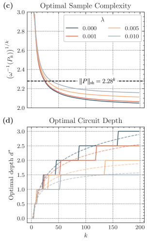
(b)

Figure 2: Sample complexity in robust shallow shadows (RSS) for Pauli observables with contiguous support of size $k$. In (a), we show a conceptual illustration of the three physical phenomena influencing sample complexity in the context of a classical random walk model: 1) operator spreading with a ‘butterfly velocity’ $v_{B}$; 2) particle density relaxation; and 3) noise-induced decay with rate $e^{-\lambda}$. These phenomena collectively determine the sample complexity required for accurate observable estimation. In (b), we illustrate the qualitative impact of noise on the sample complexity upper bound, illustrating that increased noise levels lead to a slight increase in the sample complexity upper bound and a reduction in the optimal circuit depth. This reduction is approximately linear in the noise strength $\lambda$, with a proportionality coefficient $\alpha$. This is an example of the trade-offs involved in designing a noise-robust protocol. In (c), we show the exact optimal sample complexity, computed numerically, for a variety of noise strengths. Importantly, even under the presence of noise, the sample complexity beats the $\sim 2.28^{k}$ upper bound predicted by Ref. [57]. Finally, in (d), we show the scaling of the optimal circuit depth $d^{*}$ as a function of $k$. The dashed lines correspond to theoretical predictions based on Theorem 1.

Since the shadow map (1) is diagonal in the Pauli basis, the expectation of any Pauli $P$ is simply

$$\Tr(\rho P)=\frac{1}{\omega_{\lambda}(P)}\mathbb{E}[\Tr(\hat{\sigma}P)].$$ (3)

Since $\absolutevalue{\Tr(\hat{\sigma}P)}\leq 1$, the inverse Pauli weight upper bounds the shadow norm of any Pauli $P$ (i.e., the sample complexity of estimating $P$): $\norm{P}^{2}_{\text{sh}}\leq\omega_{\lambda}(P)^{-1}$. Therefore, to upper bound the sample complexity, it suffices to lower bound the Pauli weight $\omega_{\lambda}(P)$. For our theoretical analysis, we make the simplifying assumption that the noise is single-qubit depolarizing noise with site-independent strength $\lambda$. In Ref. [57], it was shown that, in the noiseless case, the expectation in Eq. 2 can be calculated by mapping the evolution of $P$ through the circuit to a classical random walk, and the shadow norm depends on the final set of configurations in this random walk. We extend this analysis to the noisy case. As we show, the effect of noise on this random walk is simple. The picture is simplest for Pauli operators that are comprised of $k$ contiguous non-trivial characters. The random walk for this case is illustrated in Fig. 2(a). As depicted, there are three physical processes, and only the third of these depends on the noise. First, the average density of particles in the bulk will relax, owing to the fact that twirled two-qubit gates tend to reduce the weight of high weight Pauli operators (for instance, a Haar random two-qubit gate maps a weight 2 Pauli operator to a weight 1 Pauli operator with probability $\frac{3}{5}$). Second, the domain of the observable will spread (shown in red) with some butterfly velocity $v_{B}$ as a result of the entangling two-qubit gates which act on the edge of the Pauli’s support. Finally, each particle will have a damping factor of $\exp(-\lambda)$ during the stochastic process due to the depolarizing noise. The effects of each of these three processes can be bounded, and combining all of these bounds allows us to obtain an upper bound of the shadow norm for contiguous Pauli operators, hence bounding the requisite sample complexity to estimate these operators. The details of the theoretical analysis, as well as a numerical characterization of phenomenological parameters such as $\gamma$ and $v_{B}$ can be found in Appendix C.

Theorem 1 (Sample complexity and optimal circuit depth, informal).

Assuming single-qubit depolarizing noise with strength $\lambda$, for $k\gg d\gg 1$, the shadow norm of a Pauli operator support over $k$ contiguous sites is upper bounded by

$$\log_{3}\norm{P_{k}(d)}^{2}_{\mathrm{sh}}\leq\quantity(k+d)\quantity(\frac{3}{4}+\frac{\exp(-\gamma d)}{t^{3/2}}+\frac{d\lambda}{\log 3}),$$ (4)

where $d$ is the circuit depth and $\exp(-\gamma)\equiv(\frac{4}{5})^{2}$. The circuit depth $d^{*}$ that minimizes this upper bound is

$$d^{*}=\frac{1}{\gamma}\quantity(\log\frac{k}{3\log 3+4k\lambda}+\ldots)\underset{(k\lambda\ll 1)}{=}\frac{1}{\gamma}\quantity(\log\frac{k}{3\log 3}-\frac{4k\lambda}{3\log 3}+\ldots)$$ (5)

where $\ldots$ denotes subleading terms.

Eq. 5 shows that the theoretical optimal circuit depth is smaller for noisy circuits compared to noiseless ones, a fact which we visualize in Fig. 2(b). Simultaneously, Eq. 4 shows that the noise also increases the associated sample complexity for estimating $P_{k}$. However, the sample complexity bounds in this theorem are overly pessimistic, and we can do significantly better using a phenomenological model that we detail in Appendix C.

II.2 Pauli-Lindblad noise model

Although the single-qubit depolarizing noise model made our theoretical analysis simple, this model is unrealistic for most practical scenarios. For instance, it completely ignores the crosstalk and two-qubit error channels that are present in the qubit architecture that we use in this work. We model the noise channel $\Lambda$ of a $N$-qubit system from the local interactions generated by a Lindbladian $\mathcal{L}(\rho)=\sum_{k\in\mathcal{K}}\lambda_{k}\left(P_{k}\rho P_{k}-\rho\right)$, where $\mathcal{K}$ is a set of Pauli operators that is defined by the local interactions between qubits. This model is shown to be a good description of realistic hardware noise in Ref. [61]. Since these interactions are generally assumed to be nearest neighbor interactions, the size of $\mathcal{K}$ (and hence the number of noise parameters) is linear in $N$ [61]. That is, if $U$ represents a single layer of CNOT gates, the state after this layer will be $\rho^{\prime}=e^{\mathcal{L}}[U\rho U^{\dagger}]$. Since $\mathcal{L}$ is a sparse Pauli-Lindbladian, $e^{\mathcal{L}}$ enjoys a particularly simple form when acting on Pauli operators:

$$e^{\mathcal{L}}[P]=\exp(-\sum_{k;\commutator{P_{k}}{P}\neq 0}\lambda_{k})P,$$ (6)

which is to say that $P$ acquires a damping factor that depends on the Lindbladian generators with which it does not commute [61]. We assume different noise parameters $\lambda$ for the even and odd layers of CNOT gates, and model readout errors by absorbing them into the last layer of Pauli-Lindbladian noise. We note that although the Pauli-Linadblad model has 9 two-body terms for each neighboring pair of qubits and 3 on-site terms for each qubit, the single-qubit twirling in our shallow circuit ensemble simplifies this noise significantly. The effect of these random single-qubit gates is to twirl the noise such that for each edge, it can be parameterized by three numbers: $\lambda_{PI},\lambda_{IP},\lambda_{PP}$. These represent the local action of the noise channel on a Pauli operator which has support on the first qubit, second qubit, or both qubits, respectively. The first two terms can be interpreted as single-qubit depolarizing noise.

Accurate values for $\lambda$ are crucial for unbiased observable prediction. To estimate these parameters, we apply the framework of Bayesian inference. Although the probabilistic error cancellation (PEC) framework [61] can be used for this estimation as well, since the noise is twirled by random single-qubit Clifford gates, this results in a simplification of the effective noise channel. This simplification means that it is sufficient to use historical noise data (learned via PEC) as a loose prior, and to use Bayesian learning to ‘fine-tune’ this prior. This Bayesian learning method requires less device time compared to PEC, as the calibration dataset $\mathcal{D}_{c}$ we use for the parameter estimation is relatively simple. First, we collect a calibration dataset $\mathcal{D}_{c}$ simply by running our randomized measurement protocol for a state $\rho=\outerproduct{0}{0}^{\otimes N}$, which can be prepared with high fidelity. We then use this dataset to define a likelihood function $p(\mathcal{D}_{c}\mid\lambda)$ as follows. We construct an estimator for the Pauli weights $\tilde{\omega}_{\mathcal{D}_{c}}(P)$ by inverting Eq. 3:

$$\tilde{\omega}_{\mathcal{D}_{c}}(P)=\frac{1}{\absolutevalue{\mathcal{D}_{c}}\Tr(\outerproduct{0}{0}P)}\sum_{i=1}^{\absolutevalue{\mathcal{D}_{c}}}\Tr(\hat{\sigma_{i}}P),$$ (7)

where we always choose $P$ to be some tensor product of identity and $Z$ operators. Since any Pauli weight depends only on the support of $P$ (thanks to the local-basis invariance of our ensemble) this subset of operators is sufficient to capture all Pauli weights. We calculate the standard deviations $\sigma_{P}$ of these estimators using a bootstrap estimate. The likelihood function is then simply

$$p(\mathcal{D}_{c}\mid\lambda)\propto\exp(-\sum_{P}\frac{\quantity(\tilde{\omega}_{\mathcal{D}_{c}}(P)-\omega_{\lambda}(P))^{2}}{2\sigma_{P}^{2}}),$$ (8)

where the sum runs over all Paulis $P$ that are contiguous $Z$-strings up to weight 6 (beyond this weight, empirically recovered Pauli weights are too small to be resolved to within statistical significance). The prior $p(\lambda)$ is given by a log-normal distribution with $\sigma=2$, and centered around noise parameters $\tilde{\lambda}$ calculated via an independent inference process, namely that of Ref. [61]. Together, the two fully specify the posterior distribution over the noise parameters:

$$p(\lambda\mid\mathcal{D}_{c})\propto p(\mathcal{D}_{c}\mid\lambda)p(\lambda).$$ (9)

We can then sample from this posterior distribution using Hamiltonian Monte Carlo [71, 72]. Although this method essentially gives us access to the full posterior distribution, in practice, we typically pick a fixed value of $\lambda$ when inferring observables. This fixed value can be chosen a number of ways, including by taking the mean or median of the posterior distribution samples, or simply using a maximum a posteriori probability (MAP) estimate (found by maximizing Eq. 9 via gradient descent). We find that each of these three methods for fixing $\lambda$ produce almost identical results.

II.3 Tensor network-based postprocessing

In this section, we will show that we can use a tensor network to represent all $2^{N}$ Pauli weights with polynomial classical resources [14]. We begin by defining $\mathcal{C}_{2}[O]=\mathcal{C}^{\dagger}_{U,\lambda}[O]\otimes UOU^{\dagger}$, allowing us to rewrite the noisy Pauli weight from Eq. 2 as

$$\omega_{\lambda}(P)=\Tr(\outerproduct{0}{0}^{\otimes 2}\underset{U\sim\mathcal{E}}{\mathbb{E}}[\mathcal{C}_{2}[P^{\otimes 2}]]).$$ (10)

As will become clear below, the expectation in Eq. 10 can be understood as a distribution over all possible final configurations of a random walk. This random walk has as its possible states all $4^{N}$ Pauli operators, and the initial state is $P$ with probability 1. Since each of the random gates in our ensemble $\mathcal{E}$ are independently chosen, the effect of each gate can be thought of as a transition in this random walk. To illustrate this, consider the effect of single-qubit random Clifford gates (which are assumed to be noiseless). For any non-identity single-qubit Pauli operator $P$, a random single-qubit Clifford $U\sim\operatorname{Cl}(2)$ maps $P^{\otimes 2}$ to an equal superposition of $X^{\otimes 2}$, $Y^{\otimes 2}$, and $Z^{\otimes 2}$:

$$\underset{U\sim\operatorname{Cl}(2)}{\mathbb{E}}[U^{\otimes 2}P_{a}^{\otimes 2}(U^{\dagger})^{\otimes 2}]=\frac{X^{\otimes 2}+Y^{\otimes 2}+Z^{\otimes 2}}{3}\cong\frac{|X)+|Y)+|Z)}{3}.$$ (11)

The last part of the equation introduces convenient notation by representing the distribution over Paulis as a vector, using a basis $\quantity{|I),|X),|Y),|Z)}$. Then, each single-qubit random Clifford gate can be associated with a transition matrix for the random walk:

$$T=\begin{bmatrix}1&0&0&0\\ 0&1/3&1/3&1/3\\ 0&1/3&1/3&1/3\\ 0&1/3&1/3&1/3\\ \end{bmatrix}.$$ (12)

Also, the CNOT gates induce a deterministic transition $|P)\to|P^{\prime})$, where $P^{\prime}$ is the Pauli that $P$ is mapped to under the action of a CNOT. Under the action of single-qubit Cliffords and CNOT gates, the resulting distribution over Pauli strings is normalized at each step of the random walk – physically, this corresponds to the fact that we have unit purity for all noiseless circuits. However, after noise acts, our distribution becomes subnormalized. In spite of this, there is still a simple form for the noise in terms of a quasi-transition matrix $T_{\lambda}$. For instance, for single-qubit depolarizing noise, the transition matrix is $T_{\lambda}=\operatorname{diag}(1,e^{-\lambda},e^{-\lambda},e^{-\lambda})$. On the other hand, the two-body terms in the sparse Pauli-Lindbladian model result in $16\times 16$ diagonal transition matrices acting on nearest neighbors, where the entry for $P$ is simply the factor $\exp(-\sum_{k;\commutator{P_{k}}{P}\neq 0}\lambda_{k})$. This summarizes the action of each component in our unitary ensemble, and putting it together allows us to derive the (subnormalized) probability distribution $p$ over Pauli strings that represents $\mathbb{E}_{U\sim\mathcal{E}}[\mathcal{C}_{2}[P^{\otimes 2}]]$:

$$\mathbb{E}_{U\sim\mathcal{E}}[\mathcal{C}_{2}[P^{\otimes 2}]]\cong\sum_{Q\in\mathbb{P}_{N}}p(Q)|Q)\equiv|\Psi).$$ (13)

Now, note that $\Tr\quantity(\outerproduct{0}{0}^{\otimes 2}Q^{\otimes 2})$ is equal to one if and only if $Q$ is comprised entirely of identity and $Z$ operators (it is zero otherwise). Therefore, we can calculate the noisy Pauli weights by $\omega_{\lambda}(P)=(+|\Psi)$,where $(+|=\begin{bmatrix}1&0&0&1\end{bmatrix}^{\otimes N}$.

Although the above discussion uses the language of Markov chains, the $|\cdot)$ notation is suggestive of yet another layer on top of this representation. Each of the transfer matrices acts locally on the states $|P)$, mirroring the connectivity of the circuit ensemble $\mathcal{E}$. Therefore, if we represent the distribution as a vector in a $4^{N}$ dimensional Hilbert space, with basis vectors being the Pauli operators, $\mathbb{E}[\mathcal{C}_{2}[\cdot]]$ can be represented as a matrix product operator (MPO) $\tilde{C}_{2}$. Then, $|\Psi)=\tilde{C}_{2}|P)$, so we can write

$$\omega_{\lambda}(P)=(P|\tilde{C}_{2}|+)\,,\,\,\text{or simply}\,\,\omega_{\lambda}=\tilde{C}_{2}|+)$$ (14)

Therefore, by construction, the noisy Pauli weights $\omega_{\lambda}(P)$ can be represented as a matrix product state (MPS), in the Pauli basis, with bond dimension $\exp(\mathcal{O}(d))$, where $d$ is the depth of the circuit. Since the optimal circuit depth $d^{*}$ is at most logarithmic in $N$ (Theorem 1), the necessary classical resources to encode the noisy Pauli weights is $\mathcal{O}(\text{poly}(N))$. A similarly efficient MPS representation of $\omega_{\lambda}^{-1}$ can be found variationally using gradient descent [14, 15]. To predict a general physical observable $\Tr(\rho O)$, we use the estimator

$$\begin{split}\frac{1}{\absolutevalue{\mathcal{D}}\cdot 2^{n}}\sum_{i=1}^{\absolutevalue{\mathcal{D}}}\sum_{P\in\mathbb{P}_{N}}\omega_{\lambda}^{-1}(P)\Tr(\hat{\sigma}_{i}P)\Tr(OP).\end{split}$$ (15)

Evaluating (15) requires a tensor contraction of three matrix product states: $\omega_{\lambda}^{-1}$, $\hat{\sigma}_{i}$, and $O$, each of which can be thought of as vectors in the Pauli basis. For instance, if $O$ is a Pauli operator $ZXX$, it is a product state in the Pauli basis $|Z)\otimes|X)\otimes|X)$. If $O$ is $\outerproduct{0}{0}$, it is again a product state in the Pauli basis: $\outerproduct{0}{0}\cong\bigotimes_{i=1}^{N}\frac{|I)+|Z)}{2}$. Since $\omega_{\lambda}^{-1}$ and $\hat{\sigma}_{i}$ have efficient MPS representations by assumption that our ensemble of circuits $\mathcal{E}$ is log-depth, if we have an efficient MPS representation of $O$, the contraction in Eq. 15 is efficient, with a time complexity $O(N\chi_{\omega}\chi_{\sigma}\chi_{O})$, where $\chi_{\omega}$, $\chi_{\sigma}$, and $\chi_{O}$ are the bond dimensions of $\omega_{\lambda}^{-1}$, $\hat{\sigma}$, and $O$ respectively. This completes the details of our algorithm. We summarize the entire protocol in Section II.3.

[h]

III Experiments

There are a number of choices that an experimentalist is free to make in Section II.3. The first is the choice of the unitary ensemble $\mathcal{E}$. As shown in the original classical shadow framework [1], the details of this ensemble can have a drastic impact on sample complexity, depending on the observables of interest. For instance, ensembles comprised of single-qubit random Cliffords are well suited for predicting local observables, while ensembles comprised of global random Cliffords are useful for low-rank observables such as fidelity. In this section, we will provide experimental evidence showing that interpolating between these two regimes allows us to achieve, in a sense, the best of both worlds. By using shallow brickwork random Clifford circuits, we show that an extremely broad class of observables can be measured with relatively low sample complexity, including both local observables and low-rank observables such as fidelity. Concretely, we test three different ensembles which consist of $d\in\quantity{0,1,2}$ layers of single-qubit twirled CNOT gates. The $d=0$ is simply the random single-qubit Clifford case initially proposed in Ref. [1], also known simply as randomized Pauli measurements. On the other hand, as shown in Fig. 1(a), when $d=1$, our circuits contain two layers of twirled CNOT gates (one even layer and one odd layer), so $d=2$ contains four layers of twirled CNOT gates. The other remaining degrees of freedom in Section II.3 are the size of the dataset $\mathcal{D}$, the application state $\rho$, and the observables of interest. For both the calibration and application dataset, we applied $10000$ different random unitaries from $\mathcal{E}$ and took 100 shots for each unitary circuit (see Appendix D for experimental details). We then applied our multitasking protocol on both the plus state $\ket{+}^{\otimes 18}$ and a cluster state. The cluster state we choose is $\ket{\phi}=\prod_{i=1}^{N-1}\text{CZ}_{i,i+1}\ket{+}^{\otimes N}$, which is a ground state of a symmetry-protected topological (SPT) Hamiltonian $H=-\sum_{i}Z_{i-1}X_{i}Z_{i+1}$. Even though both are stabilizer states, we emphasize that our method doesn’t rely on any special properties of the stabilizer states (later in this section, we will demonstrate this by applying our protocol to the AKLT resource state). We show below that, using the same randomized measurement dataset, we can accurately predict a number of observables for each of these states, including fidelity, local and nonlocal Pauli observables, and subsystem purity.

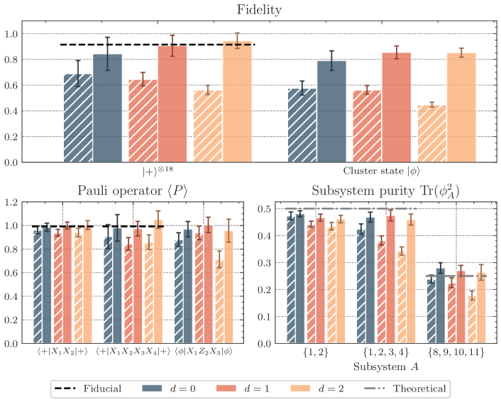
Figure 3: We apply RSS to predict multiple quantities including fidelity, Pauli observables, and subsystem purities. The hatched bars indicate recovered values without error mitigation, while the solid bars use error mitigation. In the top panel, we infer the fidelity of the experimentally prepared plus state $\ket{+}^{\otimes 18}$ and cluster state $\ket{\phi}$ with respect to the ideal (i.e., perfectly prepared) state. For the plus state, predictions agree with fiducial values obtained via direct fidelity estimation, showcasing the effectiveness of RSS in error mitigation. In contrast, predictions without error mitigation exhibit a decline in fidelity as circuit depth increases, underscoring the impact of noise. The lower left panel displays the predicted expectation values of Pauli observables, where RSS predictions maintain consistency and, for the plus state, agree with fiducial values. The lower right panel shows different subsystem purity predictions for a cluster state, illustrating how purity values are contingent upon the number of cuts within a subsystem. For instance, a subsystem in the bulk (formed by two cuts) has theoretical purity 0.25, whereas a boundary subsystem, with one cut, has a theoretical purity 0.5.

Fig. 3 summarizes our experimental results for the plus state and cluster state. The top panel shows the inferred overlap between the experimentally prepared state and the ideal application state. The hatched bars indicate recovered values without error mitigation, while the solid bars show inferred values when accounting for noise. To verify the correctness of our protocol, we also estimated some of these observables with direct measurement. For instance, the overlap of the experimentally prepared state with $\ket{+}^{\otimes 18}$ was calculated by repeatedly measuring in the $X$ basis, and the three Pauli observables were inferred similarly. The directly measured values are marked with the dashed black line. We find that all of our error mitigated inferred values are in agreement with these fiducial values.

We can also use the dataset to predict nonlinear properties, such as subsystem purity $\Tr\psi_{A}^{2}$, where $\psi_{A}$ is the reduced density matrix of $\psi$ on subsystem $A$. This purity is important because it encodes information about the entanglement entropy of a state – more specifically, it is related to the entanglement 2-Rényi entropy via $S_{2}=-\log_{2}\Tr(\psi_{A}^{2})$. The entanglement entropy of a (perfectly prepared) cluster state is well-known. The degenerate boundary edge modes are broken in the state preparation for the cluster state, but if we cut the system into two pieces, this cut will create a degenerate edge mode, which in turn creates 1 bit of information. That is, we expect that each cut will reduce purity by a factor $\frac{1}{2}$. To be more concrete, if a subsystem is created with a single cut (e.g., subsystems $\quantity{1,2}$ and $\quantity{1,2,3,4}$), then the theoretically expected subsystem purity is $\frac{1}{2}$. If a subsystem is created with two cuts (e.g., subsystem $\quantity{8,9,10,11}$), we expect the subsystem purity to be $\frac{1}{4}$. In Fig. 3, we observe that indeed the predicted purity after error mitigation is close to these theoretical values. The small deviations away from theoretical values is due to imperfect state preparation: as shown in Fig. 3, the experimentally prepared cluster state has fidelity $\sim 80\%$.

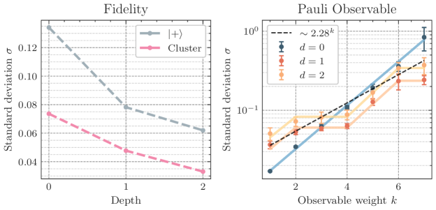
Figure 4: Sample complexity advantage of RSS. On the left, we show the decrease in the standard deviation (hence decrease in sample complexity) of fidelity predictions with increasing circuit depth. On the right, we show standard deviations for recovering Pauli operators expectations as a function of the Pauli operator weight $k$. We find excellent agreement between experimental (solid dots with error bars) and theoretical (solid lines) values. Notably, shallow circuits ($d=1,2$) have favorable sample complexity scaling for higher-weight Pauli operators, surpassing both the $d=0$ scaling (which is $3^{k}$), as well as the theoretical upper bound of $2.28^{k}$.

One of the advantages of applying shallow circuits to classical shadow tomography is the reduction of sample complexity for both nonlocal and low-rank observables. To evidence this claim, we observe two competing effects. First, as shown in Theorem 1, increased depth is well-suited for nonlocal observables. It is also well-suited for low-rank observables such as fidelity, since we converge to the global Clifford ensemble (which is optimal for low-rank observables) with increased depth. This improved suitability reduces the standard deviation of the inferred values for these observables at larger depths: this effect is particularly evident for fidelity, as highlighted in Fig. 4. However, this effect competes against the increasing effects of noise. As can be seen in Fig. 3, when error mitigation is turned off, the recovered fidelity systematically decreases with the depth $d$ – the reason for this is not that the true fidelity is decreasing, but rather that as more CNOT gates are applied, the effect of noise on the shadow tomography process begins to accumulate, which consistently decreases the quality of our observable estimates. That is, the noise introduces a bias to the recovered values, and this bias grows with increasing depth. As discussed in Section II.2, this bias can be corrected using Pauli weights $\omega_{\lambda}^{-1}$ that have been appropriately calibrated. However, this comes at the cost of slightly increased variance, which in turn increases the sample complexity. As with the bias, this increase in sample complexity also grows with depth $d$. Using experimental data, we quantitatively study the competition between these two effects in Fig. 4. Using bootstrap estimates of the standard deviation $\sigma$ of our recovered expectation values, we can study the effects of increased depth on a variety of observables, including fidelity and a set of Pauli observables with increasing weight. We observe that for high-weight Pauli observables, the two competing effects find an optimal tradeoff at $d=1$. We also note that although upper bounds from Theorem 1 predict a standard deviation $\sim 2.28^{k}$ at the optimal depth in an ideal setting (already a significant improvement over $\sigma\sim 3^{k}$, which is the scaling for $d=0$), we find that in practice, we can do much better than this, as evidenced by the $d=1$ line compared to $2.28^{k}$ dashed line. We can of course do much better than this rough fit; our MPS formalism allows us to calculate an exact prediction for the standard deviation of any Pauli observable. These predictions are shown in solid lines, demonstrating excellent agreement with the bootstrapped standard deviations. This further evidences the accuracy of our shadows protocol. Turning to the case of fidelity estimation, we see, unlike Pauli observables, $d=2$ is a strict improvement over $d=1$. This is expected, as $d=\infty$ is the optimal setting for fidelity estimation in the noiseless limit [1]. Regardless, for both Pauli observables and fidelity, using a shallow depth ensemble is always strictly better than using a $d=0$ ensemble, illustrating one of the key advantages of our method.

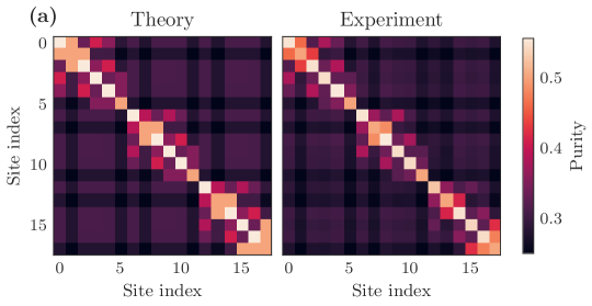
Figure 5: Prediction of subsystem purity in the AKLT resource state using RSS. In (a), we demonstrate how the RSS method can use a single dataset to concurrently predict the purity of all subsystems up to two qubits within AKLT resource states. The values at $(i,j)$ represent the purity of the reduced density matrix $\Tr(\rho_{ij}^{2})$. The AKLT resource state has three clusters, each representing a smaller AKLT state with two spin-1 particles before fusion measurement; experimental predictions clearly show this pattern as well, and closely align with theoretical predictions. In (b), we show a schematic of the AKLT resource state before fusion measurements are applied to prepare the AKLT state.

Finally, we applied RSS to predict the purity of all size 1 and 2 subsystems for the AKLT resource state on 18 qubits. This resource state is a precursor for preparing the AKLT state in constant depth; importantly, this state is not a stabilizer state [73]. As shown in Fig. 5(b), this state consists of 3 small clusters of AKLT states, which can eventually be merged into a 6-qubit AKLT state. The small clusters are knit together into a single global AKLT state by applying Bell measurements on the edge qubits of adjacent small AKLT states, and applying a correction conditioned on the measurement outcome (this process is known as applying ‘fusion measurements’). However, in this work, we do not apply these fusion measurements, as this requires measurement feedforward, which is experimentally difficult to implement. Instead, we prepare the AKLT resource state on superconducting qubits and characterize its entanglement structure, prior to fusion measurements, using RSS. In Fig. 5(a), we show theoretical and experimentally recovered values for every 1- and 2-qubit subsystem purity of the resource state. Comparing the recovered purities shows excellent agreement with exact theoretical values: as expected, we clearly see three distinct entangled clusters in the experimental data, representing each of the local AKLT states.

We note that when there is a strong mismatch between the noise model and actual device noise, the Bayesian calibration procedure could fail and lead to biased prediction. In such cases, directly using Eq. 2 can provide a model-agnostic way to estimate Pauli weights. In our experiments, however, comparison between error-mitigated shadow prediction and fiducial values from other direct measurement schemes do not show such deviations within statistical uncertainties.

IV Outlook

In this work, we executed an unbiased randomized measurement experiment that went beyond random Pauli measurements for large quantum systems. In these experiments, we showed that our robust shallow shadow protocol can efficiently recover unbiased estimates for a wide array of observables on unknown quantum states, even under the presence of noise. We do this by providing a general noise characterization technique based on Bayesian inference that can account for realistic noise effects, such as qubit crosstalk and measurement error. Having characterized the noise on our device, we then introduced an efficient tensor network-based postprocessing technique that is naturally able to account for the effects of this noise. We provide evidence that this error mitigation technique is effective by demonstrating that our protocol gives unbiased predictions of low-rank observables (e.g., fidelity), nonlocal Pauli observables, and even non-linear observables (e.g., subsystem purity) for a number of application states, including the cluster state and the AKLT resource state. Not only is our protocol able to recover unbiased estimators of these observables, we show that the standard deviation of these estimators decreases with increasing depth. That is, we show how going beyond random Pauli measurements can give rise to improved sample complexities. Furthermore, we developed a theoretical framework that not only predicted improvements in sample complexity that agreed well with the empirically observed improvements, but our framework also showed that shallow shadows remain information-theoretically optimal, even under the presence of noise. Our new theoretical insights, combined with the experimental validation of our protocol, further underscores the practical relevance and effectiveness of our approach. The success of these experiments not only validates the theoretical underpinnings of our protocol but also showcases its potential for real-world quantum computing applications.

We believe our new method has many applications in quantum machine learning, quantum chemistry, and quantum many-body physics. The randomized measurements dataset serves as a succinct classical description of a quantum state. By predicting many different Pauli observables efficiently, one can do unsupervised learning of conserved quantities, symmetry, and phases of matter for quantum many-body systems [74, 75, 55]. A similar approach can be used for ansatz-free Hamiltonian learning and quantum device benchmarking [76, 43, 77]. Measuring many low-rank observables simultaneously could also lead to new applications. For example, estimating the low eigenenergy spectrum is important for quantum many-body physics and quantum chemistry. Combining the idea of dynamic mode decomposition [78] and measuring many low-rank observables simultaneously, one could have a better convergence rate in predicting eigenenergies. Last but not least, it would be interesting to use modern machine learning techniques further to improve the inference and predictions of the proposed method [79] and also improve the sample complexity by tailoring unitary ensembles to special observables of interest [36, 32].

Note added — During the completion of this manuscript, we became aware of a related but independently developed work taking a randomized benchmarking approach to mitigate noise in randomized measurements. [80].

V Acknowledgements

We would like to thank Gefen Baranes, Pablo Bonilla, Nazlı Uğur Köylüoğlu, and Varun Menon for insightful discussions. SFY and HYH thank the NSF for funding through the QIdeas HDR and the CUA PFC. YZY is supported by the NSF Grant No. DMR-2238360.

VI Data Avialability

Source data are available for this paper. All other data supporting the plots within this paper and other study findings are available from the corresponding author upon reasonable request.

VII Code Availability

The code used in this study is available from the corresponding author upon request.

VIII Author Contributions

H.Y.H and A.G. developed the theory of robust shallow shadows and wrote the code for the analysis of experimental data. S.M. conducted the experiments and collected the randomized measurement dataset. A.G. conducted the data postprocessing of the experimental data. H.Y.H, Y.Z.Y, S.F.Y., A.S., and Z.M. designed the application and experiments. All authors contributed substantially in writing the manuscript.

Supplementary Material

Appendix A Locally scrambled classical shadow with general quantum channel

In the following discussion, we assume any two-qubit or multi-qubit gates are sandwiched by random single-qubit Clifford gates. This operation is also called “single-qubit twirling”. Any circuit composed entirely of single-qubit twirled gates is called a locally scrambled circuit. Mathematically, a unitary ensemble is called locally-scrambled if $P(U)$ satisfies local-basis invariance condition

$$P(U)=P(VU)=P(UV),\quad\forall V\in U(2)^{N},$$ (16)

where $V\in U(2)^{N}$ denotes the fact that $V$ is a tensor product of $N$ local unitaries [12]. Since every two-qubit or multi-qubit gates are twirled by random single-qubit Clifford gate, $\mathcal{C}_{P}$ has the local scrambling property. In classical shadow experiments, the unitary evolution channel $U$ is different each time, and sampled from the unitary ensemble $\mathcal{E}_{U}$. Therefore, we explicitly use $\mathcal{C}_{U,P}$ and $\mathcal{C}_{U,V}$ to show the unitary $U$ dependence.

The classical snapshots are

$$\begin{split}\hat{\sigma}_{U,b}=\mathcal{C}^{\dagger}_{U,V}[\ket{b}\bra{b}],\end{split}$$ (17)

and the probability of getting it is

$$\begin{split}p(\hat{\sigma}_{U,b}|\rho)=\Tr(\ket{b}\bra{b}\mathcal{C}_{U,P}[\rho]).\end{split}$$ (18)

It can be shown that under the locally scrambling assumption, the measurement channel is diagonal in the Pauli basis,

$$\begin{split}\mathcal{M}[\rho]&=\underset{U}{\mathbb{E}}\sum_{b}\hat{\sigma}_{U,b}p(\hat{\sigma}_{U,b}|\rho)\\ &=\dfrac{1}{2^{n}}\sum_{P\in\mathbb{P}_{n}}\omega(P)\Tr(\rho P)P,\end{split}$$ (19)

where $\omega(P)$ is the Pauli weight of Pauli string $P$, and

$$\begin{split}\omega(P)&=\dfrac{1}{2^{n}}\sum_{b}\underset{U}{\mathbb{E}}\left(\Tr(\mathcal{C}^{\dagger}_{U,V}[\ket{b}\bra{b}]P)\Tr(\mathcal{C}^{\dagger}_{U,P}[\ket{b}\bra{b}]P)\right).\end{split}$$ (20)

When both $\mathcal{C}_{U,V}$ and $\mathcal{C}_{U,P}$ are the same unitary channel, it returns to the original locally scrambled classical shadows. Since both the quantum channel $\mathcal{C}_{U,V}$ and $\mathcal{C}_{U,P}$ have local basis invariance property, the dependence on different bit-string state $\ket{b}$ is spurious. We can simplify the Pauli weight as

$$\begin{split}\omega(P)&=\underset{U}{\mathbb{E}}\Tr\left(\mathcal{C}^{\dagger}_{U,V}[\ket{0}\bra{0}^{\otimes N}]P\right)\Tr\left(\mathcal{C}^{\dagger}_{U,P}[\ket{0}\bra{0}^{\otimes N}]P\right)\\ &=\underset{U}{\mathbb{E}}\Tr\left(\ket{0}\bra{0}^{\otimes N}\mathcal{C}_{U,V}[P]\right)\Tr\left(\ket{0}\bra{0}^{\otimes N}\mathcal{C}_{U,P}[P]\right).\end{split}$$ (21)

One can also define $\mathcal{C}_{U}=\mathcal{C}_{U,V}\otimes\mathcal{C}_{U,P}$, and written the Pauli weight as

$$\begin{split}\omega(P)&=\underset{U}{\mathbb{E}}\Tr\left(\ket{0}\bra{0}^{\otimes 2N}\mathcal{C}_{U}[P^{\otimes 2}]\right).\end{split}$$ (22)

In the post-processing, one usually uses the ideal unitary evolution, i.e. $\mathcal{C}_{U,V}[\cdot]=U\cdot U^{\dagger}$, and the corresponding physical channel in the experiment is noisy, the Pauli weight

$$\begin{split}\omega(P)=\underset{U}{\mathbb{E}}\Tr\left(\ket{0}\bra{0}^{\otimes N}UPU^{\dagger}\right)\Tr\left(\ket{0}\bra{0}^{\otimes N}\mathcal{C}_{U,P}[P]\right)\end{split}$$ (23)

is also related to the randomized benchmarking [81]. In Appendix B, we will develop a tensor-network based method that can efficiently calculate Pauli weight (23) using Polynomial classical resources, and also demonstrate how to use the method to estimate nonlocal properties, such as quantum state fidelity.

Appendix B Tensor network post-processing for robust shallow shadow

B.1 Noise-free circuit Pauli weight calculation

Let’s start with the noise-free shallow circuit shadows, where both $\mathcal{C}_{U,V}[\cdot]=\mathcal{C}_{U,P}[\cdot]=U\cdot U^{\dagger}$. Suppose the system comprises a single qubit, the Pauli weight is

$$\begin{split}\omega(P)=\underset{U}{\mathbb{E}}\Tr\left(\ket{0}\bra{0}^{\otimes 2}U^{\otimes 2}P^{\otimes 2}U^{\dagger\otimes 2}\right).\end{split}$$ (24)

One should be aware that the tensor product of two replicas differs from that of different qubits. When it is necessary, we will add superscripts $(1)$ and $(2)$ to explicitly denote the two replicas and use subscripts to denote the number of qubit. For example $P_{(1,2)}^{\otimes 2}=X^{(1)}_{1}\otimes X^{(2)}_{1}\otimes Y^{(1)}_{2}\otimes Y^{(1)}_{2}$. A helpful picture is to track the ”distribution” (induced by our distribution over $U$) of Pauli operators as we evolve forward under the random quantum circuit. For example, after applying one layer of single-qubit random Haar/Clifford twirling gates, a given Pauli, say $Z$, will be mapped to an equal superposition of $X$, $Y$ and $Z$. Rigorously, this is captured by the fact that

$$\begin{split}\mathbb{E}_{U\sim\text{Haar}_{1}}\left[U^{\otimes 2}Z^{\otimes 2}(U^{\dagger})^{\otimes 2}\right]=\dfrac{X^{(1)}\otimes X^{(2)}+Y^{(1)}\otimes Y^{(2)}+Z^{(1)}\otimes Z^{(2)}}{3}=-\dfrac{1}{3}I+\dfrac{2}{3}S,\end{split}$$ (25)

where $I$ is the identity operator and $S$ is the swap operator between two copies. Generally, if the distribution of $U$ is global Haar/Clifford, one has

$$\begin{split}\mathbb{E}_{U\sim\text{Haar}_{n}}\left[U^{\otimes 2}P^{\otimes 2}(U^{\dagger})^{\otimes 2}\right]=\left(\dfrac{\Tr(P)-2^{-n}\Tr(PS)}{2^{2n}-1}\right)I+\left(\dfrac{\Tr(PS)-2^{-n}\Tr(P)}{2^{2n}-1}\right)S.\end{split}$$ (26)

If the ensemble of $U$ is locally scrambled, it doesn’t distinguish different Pauli bases, and the coefficients of $X$, $Y$, and $Z$ are equal. Therefore, it is easier to work with the $I$ and $S$ basis. We use a vector notation, $\ket{I}$ and $\ket{S}$, to denote the identity and swap basis, and one should be aware that they are not superoperator notations. For example, using this vector notation, Eq. 25 can be written as

$$\begin{split}\mathbb{E}_{U\sim\text{Haar}_{1}}\left[U^{\otimes 2}Z^{\otimes 2}(U^{\dagger})^{\otimes 2}\right]=-\dfrac{1}{3}\ket{I}+\dfrac{2}{3}\ket{S}=\begin{bmatrix}-\frac{1}{3}\\ \frac{2}{3}\end{bmatrix}.\end{split}$$ (27)

Applying Eq. 26, it is easy to verify that the application of two-qubit random Haar/Clifford random unitaries has the following action:

$$\begin{split}\ket{II}&\rightarrow\ket{II}\\ \ket{SS}&\rightarrow\ket{SS}\\ \ket{IS}&\rightarrow\dfrac{2}{5}\left(\ket{II}+\ket{SS}\right)\\ \ket{SI}&\rightarrow\dfrac{2}{5}\left(\ket{II}+\ket{SS}\right),\end{split}$$ (28)

which in matrix form reads

$$\begin{split}T_{12}=\begin{bmatrix}1&0&0&0\\ \frac{2}{5}&0&0&\frac{2}{5}\\ \frac{2}{5}&0&0&\frac{2}{5}\\ 0&0&0&1\end{bmatrix}.\end{split}$$ (29)

And we name the action matrix $T$ the transfer matrix. Using transfer matrices, it is easier to keep track of the distribution of our Pauli operator $P$ under random unitary gates. When the shallow circuit comprises two-qubit random Haar unitaries with a brickwall structure, the transformation is a tensor network comprised of nearest neighbor transfer matrix $T_{i,i+1}$. At the end, we have

$$\begin{split}\mathbb{E}_{U}\left[U^{\otimes 2}P^{\otimes 2}(U^{\dagger})^{\otimes 2}\right]\equiv\ket{\Phi}=c_{1}\ket{II\dots}+c_{2}\ket{IS\dots}+\cdots+c_{2^{n}}\ket{SS\dots}.\end{split}$$ (30)

Since $\Tr\left(\ket{0}\bra{0}^{\otimes 2n}O\right)=1$ for any $O$ that is a tensor product of identities and swaps, the Pauli weight of $P$ reduces to $\omega(P)=\sum_{i}c_{i}$, which can be evaluated by calculating inner product $\innerproduct{+}{\Phi}$, where $\ket{+}\equiv\begin{bmatrix}1\\ 1\end{bmatrix}^{\otimes n}$. This algorithm has been implemented with PyClifford [82] and Tensornetwork [83].

B.2 Noisy circuit Pauli weight calculation

When the two-qubit gates are not random Haar/Clifford, the distribution of Paulis after applying those gates will not be equally distributed in $X$, $Y$ and $Z$ direction. For example, the two-qubit gates in our experiments are CNOT gates twirled by single-qubit random Clifford gates. Unlike Haar random unitaries, the CNOT gates pick a preferred direction for Paulis, in the sense that they treat $X$ and $Z$ differently. Furthermore, our local correlated Lindbladian noise model treats different Pauli basis differently. So rather than working with identity $I$ and SWAP $S$ basis, we work with a four-state system, with basis states being the Paulis $\ket{I}$, $\ket{X}$, $\ket{Y}$, $\ket{Z}$. For instance, $\ket{Z}\equiv\begin{bmatrix}0&0&0&1\end{bmatrix}^{T}$. One should notice that the defined basis is different from superoperator basis. Then, the transfer matrix of a single-qubit twirling gate is

$$\begin{split}T=\begin{bmatrix}1&0&0&0\\ 0&\frac{1}{3}&\frac{1}{3}&\frac{1}{3}\\ 0&\frac{1}{3}&\frac{1}{3}&\frac{1}{3}\\ 0&\frac{1}{3}&\frac{1}{3}&\frac{1}{3}\\ \end{bmatrix}.\end{split}$$ (31)

The transfer matrix of a CNOT gate is a $16\times 16$ matrix defined by

$$T_{\mathrm{CNOT}}[P_{i},P_{j}]=\begin{cases}1&\mbox{\quad if $P_{j}=\mathrm{CNOT}\cdot P_{i}\cdot\mathrm{CNOT}$ up to some phase\quad}\\ 0&\mbox{\quad otherwise.\quad}\end{cases}$$ (32)

Now, we also have a nice way of exactly solving Pauli distributions through noise channel, since the noise model is diagonal in the Pauli basis. For instance, if a qubit has single-qubit error rates $\lambda_{X}$, $\lambda_{Y}$, $\lambda_{Z}$, the transfer matrix of the noise channel for this site is

$$\begin{split}\Lambda=\operatorname{diag}(1,\exp(-2(\lambda_{Y}+\lambda_{Z})),\exp(-2(\lambda_{X}+\lambda_{Z}),\exp(-2(\lambda_{X}+\lambda_{Y}))).\end{split}$$ (33)

We can do the same for two-qubit noise, where our channel is then represented by a diagonal $16\times 16$ matrix. At the end, our state $\ket{\Phi}$ will be a superposition over all Paulis. The only nonzero contributions to (2) are those where all the Pauli characters are either $I$ or $Z$. So, we can evaluate (2) with $\innerproduct{+}{\Phi}$ where

$$\ket{+}=\matrixquantity[1\\ 0\\ 0\\ 1]^{\otimes n}.$$ (34)

This algorithm has also been implemented with PyClifford [82] and Tensornetwork [83].

Appendix C Optimal circuit depth of robust shallow shadows

In predicting Pauli observable $P_{\alpha}$ with classical shadows $\hat{\sigma}_{U,b}$, the inverse Pauli weight $\omega(P_{\alpha})$ serves as a rescaling factor,

$$\begin{split}\Tr(\rho P_{\alpha})=\dfrac{1}{\omega(P_{\alpha})}\mathbb{E}_{\hat{\sigma}_{U,b}}\Tr(\hat{\sigma}_{U,b}P_{\alpha}).\end{split}$$ (35)

Therefore, $\text{Var}(\Tr(\rho P_{\alpha}))=\frac{1}{\omega(P_{\alpha})^{2}}\text{Var}(\Tr(\hat{\sigma}_{U,b}P_{\alpha}))$. And it is not hard to show the shadow norm $\norm{P_{\alpha}}_{\text{shadow}}=\frac{1}{\omega(P_{\alpha})}$. Therefore, if one can calculate the Pauli weight $\omega(P_{\alpha})$, then the sample complexity of predicting Pauli observable $P_{\alpha}$ is known. Let’s start by reviewing how to estimate Pauli weight $\omega(P_{\alpha})$ for brickwall shallow circuit when no noise is present and get the optimal circuit depth. Then, the analysis is extended to the noisy circuit case.

The shadow norm of a Pauli operator of size $k$ is given by

$$\begin{split}\omega(P_{k})&=\int dU\bra{0}UP_{k}U^{\dagger}\ket{0}^{2}=\int dU\bra{0}P_{k}(t)\ket{0}^{2}\\ &=\int dU\bra{0}\sum_{l}\alpha_{l,k}(t)P_{l}\ket{0}^{2}=\int dU\int d\Psi\bra{\Psi}\sum_{l}\alpha_{l,k}(t)P_{l}\ket{\Psi}^{2}\\ &=\sum_{l}\overline{|\alpha_{l,k}(t)|^{2}}\left(\frac{1}{3}\right)^{l}=\mathbb{E}\left[\left(\dfrac{1}{3}\right)^{l}\right]\geq\left(\frac{1}{3}\right)^{\bar{l}}.\end{split}$$ (36)

where $\overline{\cdots}=\int dU[\cdots]$ and $\bar{l}$ is the average length of the evolved Pauli operator. The coefficient $\overline{|\alpha_{l,k}(t)|^{2}}$ can be viewed as the probability of having a weight $l$ Pauli operator in the evolution $P_{k}(t)=UP_{k}U^{\dagger}$. Therefore, each onsite non-trivial Pauli will have a contribution of $1/3$ in the Pauli weights. Since we are not distinguishing Pauli $X,Y,Z$, we can treat all non-trivial Paulis as a particle and identity as a hole . The random two-qubit gate will keep identity matrix still as identity, but transfer any ($2^{4}-1$) non-trivial Pauli operators to equal distributed non-trivial Pauli operators: $T\ket{\leavevmode\hbox to6.03pt{\vbox to6.03pt{\text{[drawing]}}}\leavevmode\hbox to6.43pt{\vbox to6.43pt{\text{[drawing]}}}}=a\ket{\leavevmode\hbox to6.03pt{\vbox to6.03pt{\text{[drawing]}}}\leavevmode\hbox to6.43pt{\vbox to6.43pt{\text{[drawing]}}}}+a\ket{\leavevmode\hbox to6.43pt{\vbox to6.43pt{\text{[drawing]}}}\leavevmode\hbox to6.03pt{\vbox to6.03pt{\text{[drawing]}}}}+(1-2a)\ket{\leavevmode\hbox to6.03pt{\vbox to6.03pt{\text{[drawing]}}}\leavevmode\hbox to6.03pt{\vbox to6.03pt{\text{[drawing]}}}}$, where $a=(2^{2}-1)/(2^{4}-1)=1/5$. Therefore, the transfer matrix of two-qubit Haar unitary in the particle-hole basis ($\ket{\leavevmode\hbox to6.43pt{\vbox to6.43pt{\text{[drawing]}}}\leavevmode\hbox to6.43pt{\vbox to6.43pt{\text{[drawing]}}}},\ket{\leavevmode\hbox to6.03pt{\vbox to6.03pt{\text{[drawing]}}}\leavevmode\hbox to6.43pt{\vbox to6.43pt{\text{[drawing]}}}},\ket{\leavevmode\hbox to6.43pt{\vbox to6.43pt{\text{[drawing]}}}\leavevmode\hbox to6.03pt{\vbox to6.03pt{\text{[drawing]}}}},\ket{\leavevmode\hbox to6.03pt{\vbox to6.03pt{\text{[drawing]}}}\leavevmode\hbox to6.03pt{\vbox to6.03pt{\text{[drawing]}}}}$) is

$$\begin{split}T=\matrixquantity[1&0&0&0\\ 0&a&a&a\\ 0&a&a&a\\ 0&1-2a&1-2a&1-2a].\end{split}$$ (37)

Using $T$, one can construct the transfer matrix $T_{\text{layer}}$ associated with one layer of even-odd two-qubit gates. The relaxation of the bulk particle density is determined by the eigen-modes(eigenstates) and eigenvalues of $T_{\text{layer}}$. When $m$ layers are applied to all particle state $T_{\text{layer}}^{m}\ket{\cdots\leavevmode\hbox to6.03pt{\vbox to6.03pt{\text{[drawing]}}}\leavevmode\hbox to6.03pt{\vbox to6.03pt{\text{[drawing]}}}\leavevmode\hbox to6.03pt{\vbox to6.03pt{\text{[drawing]}}}\leavevmode\hbox to6.03pt{\vbox to6.03pt{\text{[drawing]}}}\cdots}$, the eigen-modes with eigenvalues that are less than one will decay and vanishes. So to study the relaxation of the bulk density, one only needs to study the non-trivial eigen-mode associated with the largest eigenvalue, which is one when there is no noise in the circuit. All hole state $\ket{\cdots\leavevmode\hbox to6.43pt{\vbox to6.43pt{\text{[drawing]}}}\leavevmode\hbox to6.43pt{\vbox to6.43pt{\text{[drawing]}}}\leavevmode\hbox to6.43pt{\vbox to6.43pt{\text{[drawing]}}}\leavevmode\hbox to6.43pt{\vbox to6.43pt{\text{[drawing]}}}\cdots}$ is the trivial eigen-mode. The non-trivial eigen-mode with eigenvalue equals to one is $\ket{\psi}\propto 3\ket{\cdots\leavevmode\hbox to6.03pt{\vbox to6.03pt{\text{[drawing]}}}\leavevmode\hbox to6.43pt{\vbox to6.43pt{\text{[drawing]}}}\cdots}+3\ket{\cdots\leavevmode\hbox to6.43pt{\vbox to6.43pt{\text{[drawing]}}}\leavevmode\hbox to6.03pt{\vbox to6.03pt{\text{[drawing]}}}\cdots}+9\ket{\cdots\leavevmode\hbox to6.03pt{\vbox to6.03pt{\text{[drawing]}}}\leavevmode\hbox to6.03pt{\vbox to6.03pt{\text{[drawing]}}}\cdots}+\cdots$. Using mean-field analysis, one can check the probability of having a particle onsite at equilibrium is $3/4$. The second largest eigenvalue of $T_{\text{layer}}$ will determine the relaxation rate $\gamma$. Finally, the bulk relaxation can be written as

$$\begin{split}n(t)=\dfrac{3}{4}+\dfrac{1}{4}e^{-\gamma t},\end{split}$$ (38)

where $n(t)$ is the average particle density at time $t$.

C.1 Exact upper bound

In the limit of $k\gg t\gg 1$, by mapping the transfer matrix model to a classical random walk model, the authors of Ref.[57] showed that

$$\begin{split}n(t)=\dfrac{3}{4}+t^{-3/2}e^{-\gamma t},~{}e^{-\gamma}\equiv\left(\dfrac{4}{5}\right)^{2}.\end{split}$$ (39)

Therefore, the average particle length $\mathbb{E}[l]$ of after depth $t$ starting with $k$ particles is

$$\begin{split}\mathbb{E}[l]=\left(\dfrac{3}{4}+t^{-3/2}e^{-\gamma t}\right)(k+2V_{b}t),\end{split}$$ (40)

where $V_{b}$ captures the linear spreading of the operator size. For simplicity, we model the noise as a local depolarizing channel with parameter $\lambda$. Therefore, the presence of noise further introduces a decay factor $e^{-\lambda}$ that penalizes every non-identity Paulis or particle along the stochastic evolution.

$$\omega_{t}(P_{k})=\mathbb{E}\left[\left(\dfrac{1}{3}\right)^{l_{t}}\exp\left(-\lambda\sum_{i=1}^{t}l_{i}\right)\right].$$ (41)

We can find a lower bound of the Pauli weight for this by upper bounding $\sum_{i=1}^{t}l_{i}\leq\sum_{i=1}^{t}k+2i\leq kt+t^{2}$, since the support of the Pauli observable grows by at most 2 every layer of the brickwall circuit. Applying this bound and the Jensen’s inequality, we have

$$\begin{split}\omega_{t}(P_{k})\geq\exp(-\lambda(kt+t^{2}))\left(\dfrac{1}{3}\right)^{\mathbb{E}[l]}.\end{split}$$ (42)

In summary,

$$\omega_{t}(P_{k}) \geq\exp(-\lambda(kt+t^{2})-\log(3)\quantity[\quantity(\frac{3}{4}+t^{-3/2}\quantity(\frac{4}{5})^{2t})\quantity(k+2v_{B}t)])$$ (43a)

$$\geq\exp(-(k+t)\quantity[\lambda t+\log(3)\quantity(\frac{3}{4}+t^{-3/2}\quantity(\frac{4}{5})^{2t})])$$ (43b)

C.2 Phenomenological model

It turns out that using Jensen’s inequality to bound Eq. 41 is far too pessimistic. We can do significantly better by rewriting

$$\omega_{t}(P_{k})=\mathbb{E}\quantity[\exp(-l_{t}\log 3-\lambda\sum_{i=1}^{t}l_{i})].$$ (44)

We define $X(t)=-l_{t}\log 3-\lambda\sum_{i=1}^{t}l_{i}$, and model this as a normal distribution with mean $\mu_{k}(t)$ and variance $\sigma^{2}_{k}(t)$. Then, $\omega_{t}$ is the expectation of a log-normal distribution, which can be calculated in closed form: $\omega_{t}(P_{k})=\mathbb{E}[\exp(X)]=\exp(\mu_{k}(t)+\sigma_{k}^{2}(t)/2)$; we note that Jensen’s inequality corresponds to the bound $\mathbb{E}[\exp(X)]\geq\exp(\mu_{k}(t))$, so we can get significant improvements in our bounds by appropriately accounting for $\sigma_{k}^{2}(t)$. Estimating $\omega_{t}$ reduces to modeling $\mu_{k}(t)$ and $\sigma_{k}(t)$ phenomenologically. We start with $\mu_{k}(t)$: $\mathbb{E}[X]=-\log 3\cdot\mathbb{E}[l_{t}]-\lambda\sum_{i=1}^{t}\mathbb{E}[l_{i}]$. The expectation of the particle length $l_{t}$ is modeled extremely well by the ‘relaxation’ and ‘spreading’ effects described in [57]:

$$\mathbb{E}[l_{t}]=\underbrace{(k+V_{b}t)}_{\text{Spreading}}\underbrace{\quantity(\frac{3}{4}+\frac{1}{4}\exp(-t/t_{0}))}_{\text{Relaxation}},$$ (45)

where $k$ is the initial operator size, $V_{b}$ is some ‘butterfly velocity’, and $t_{0}$ is some typical timescale for the relaxation of the occupation towards the equilibrium value $\frac{3}{4}$. Therefore,

$$\mu_{k}(t) =-\log 3\cdot\frac{k+V_{b}t}{4}\quantity(3+\exp(-t/t_{0}))-\frac{\lambda}{4}\sum_{i=1}^{t}\quantity(k+V_{b}i)\quantity(3+\exp(-i/t_{0}))$$ (46a)

$$\geq-\log 3\cdot\frac{k+V_{b}t}{4}\quantity(3+\exp(-t/t_{0}))-\frac{3\lambda}{4}\quantity(kt+V_{b}t\cdot(t+1)/2)-\frac{\lambda}{4}\int_{0}^{\infty}(k+V_{b}t^{\prime})\exp(-t^{\prime}/t_{0})\differential{t^{\prime}}$$ (46b)

$$=-\log 3\cdot\frac{k+V_{b}t}{4}\quantity(3+\exp(-t/t_{0}))-\frac{\lambda}{4}\quantity(3\quantity(kt+V_{b}t\cdot(t+1)/2)+V_{b}t_{0}^{2}+kt_{0})$$ (46c)

$$\geq-\log 3\cdot\frac{k+V_{b}t}{4}\quantity(3+\exp(-t/t_{0}))-3\lambda t\quantity(kt+V_{b}(t+1)/2)\mbox{\quad(since $t_{0}=0.65$)\quad}$$ (46d)

$$\geq-\quantity(k+V_{b}t)\quantity(\frac{\log 3}{4}(3+\exp(-t/t_{0}))+3\lambda t).$$ (46e)

The variance $\sigma_{k}^{2}(t)$, in theory, depends on both $l_{t}$ as well as the sum $\sum_{i=1}^{t}l_{i}$, and covariances between the two. However, since we typically assume $\lambda\sim 10^{-2}$ while $\log 3\sim 1$, we ignore the contribution of $\lambda$. Furthermore, since $l_{t}$ and $\sum_{i=1}^{t}l_{i}$ have positive correlation, ignoring the contribution from $\sum_{i}l_{i}$ can only result in an underestimate of the variance, hence an underestimate of $\omega_{t}(P_{k})$ – since we are interested only in lower bounding $\omega_{t}(P_{k})$, we can do this freely. We find empirically that the variance of $l_{t}$ is well-described by an initial fast period of growth that saturates at some value which depends linearly on $k$, and is then followed by linear growth. That is,

$$\text{var}(l_{t})=(mk+b)(1-\exp(-t))+V^{\prime}t.$$ (47)

Figure 6: Phenomenology for the random walk model in Eq. 41. We model distribution of particle length $l_{t}$ at a given time step as a normal distribution. The shadow norm $\omega(P_{k}(t))$ is then the expectation of a log-normal distribution, which can be calculated exactly; theoretical predictions based on this model are shown in solid lines, while the circle markers indicate simulated values obtained via Monte Carlo simulation of the random walk.

Putting this together, we have

$$\omega_{t}(P_{k})\geq\exp(-\quantity(k+V_{b}t)\quantity(\frac{\log 3}{4}(3+\exp(-t/t_{0}))+3\lambda t)+\frac{(\log 3)^{2}(mk+b)(1-\exp(-t))+V^{\prime}t}{2}).$$ (48)

These results are compiled in Fig. 6.

Appendix D Experimental platform

We perform all experiments on ibm_kyiv [84], a 127-qubit superconducting quantum processor. We choose a chain of 18 qubit whose properties are shown in Fig. 7. All the circuits are decomposed into the device’s native gateset composed of the two-qubit entangling Echoed-Cross Resonance (ECR) gate, $1/\sqrt{2}(IX-XY)$ that is locally equivalent to controlled-NOT, and single qubit gates $\sqrt{X}$ (SX) and arbitrary rotations in the $Z$ basis. All the ECR gates are performed in 561.778 nanoseconds. The speed of device as characterized by Circuit Layer Operations Per Second (CLOPS) is 5000, which crucially enables fast sampling over many different circuits [85]. For each application circuit and fixed depth of Cliffords, we applied 10000 different random unitaries and measured 100 shots each. It took us, on average, 6 minutes of quantum hardware usage time to collect these 1 million samples. The experiments corresponding to $\ket{+}^{\otimes 18}$ and $\ket{\phi}$ in Figs. 3 and 4 were performed on December 21^th, 2023 and those for the AKLT state correponding to Fig. 5 were performed on February 6^th, 2024.

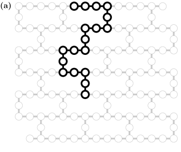
(a)

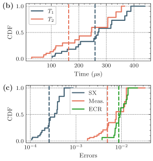
(b)

Figure 7: Experimental implementation details. In (a), we show the device layout of ibm_kyiv where 127 qubits are organized in a heavy-hex architecture. The chosen 18 qubit string is highlighted. In (b), we plot the cumulative distribution of $T_{1}$ and $T_{2}$ coherence times of the chosen qubits and in (c) we plot the single qubit gate (SX), two qubit entangling gate (ECR) and readout error rates.

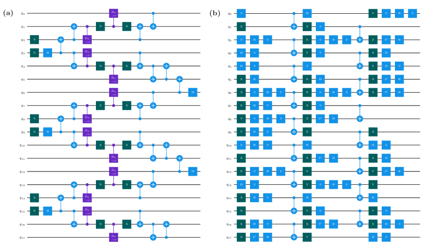
Figure 8: In (a), we show the AKLT resource state preparation circuit. In (b), we show one instance of a circuit sampled from our shallow circuit ensemble ($d=1$).

References

- Huang et al. [2020] H.-Y. Huang, R. Kueng, and J. Preskill, Nature Physics 16, 1050 (2020).
- Notarnicola et al. [2023] S. Notarnicola, A. Elben, T. Lahaye, A. Browaeys, S. Montangero, and B. Vermersch, New Journal of Physics 25, 10.1088/1367-2630/acfcd3 (2023).
- Elben et al. [2023] A. Elben, S. T. Flammia, H.-Y. Huang, R. Kueng, J. Preskill, B. Vermersch, and P. Zoller, Nature Reviews Physics 5, 9 (2023).
- Haah et al. [2017] J. Haah, A. W. Harrow, Z. Ji, X. Wu, and N. Yu, IEEE Transactions on Information Theory 10.1109/tit.2017.2719044 (2017).
- O’Donnell and Wright [2015] R. O’Donnell and J. Wright, Efficient quantum tomography (2015), arXiv:1508.01907 [quant-ph] .
- Flammia et al. [2012] S. T. Flammia, D. Gross, Y.-K. Liu, and J. Eisert, New Journal of Physics 14, 095022 (2012).
- Chen et al. [2021] S. Chen, W. Yu, P. Zeng, and S. T. Flammia, PRX Quantum 2, 030348 (2021).
- Enshan Koh and Grewal [2022] D. Enshan Koh and S. Grewal, Quantum 6, 776 (2022).
- Huang et al. [2021] H.-Y. Huang, R. Kueng, and J. Preskill, Phys. Rev. Lett. 127, 030503 (2021).
- Zhao et al. [2021] A. Zhao, N. C. Rubin, and A. Miyake, Phys. Rev. Lett. 127, 110504 (2021).
- Hu and You [2022] H.-Y. Hu and Y.-Z. You, Physical Review Research 4, 013054 (2022).
- Hu et al. [2023] H.-Y. Hu, S. Choi, and Y.-Z. You, Physical Review Research 5, 023027 (2023).
- Bu et al. [2024] K. Bu, D. E. Koh, R. J. Garcia, and A. Jaffe, npj Quantum Information 10, 6 (2024).
- Akhtar et al. [2023] A. A. Akhtar, H.-Y. Hu, and Y.-Z. You, Quantum 7, 1026 (2023).
- Bertoni et al. [2023] C. Bertoni, J. Haferkamp, M. Hinsche, M. Ioannou, J. Eisert, and H. Pashayan, Shallow shadows: Expectation estimation using low-depth random clifford circuits (2023), arXiv:2209.12924 [quant-ph] .
- Nguyen et al. [2022] H. C. Nguyen, J. L. Bönsel, J. Steinberg, and O. Gühne, Phys. Rev. Lett. 129, 220502 (2022).
- Zhou and Liu [2023] Y. Zhou and Q. Liu, Quantum 7, 1044 (2023).
- Zhou and Zhang [2023] T.-G. Zhou and P. Zhang, Efficient classical shadow tomography through many-body localization dynamics (2023), arXiv:2309.01258 [quant-ph] .
- Wu and Koh [2023] B. Wu and D. E. Koh, Error-mitigated fermionic classical shadows on noisy quantum devices (2023), arXiv:2310.12726 [quant-ph] .
- Elben et al. [2018] A. Elben, B. Vermersch, M. Dalmonte, J. I. Cirac, and P. Zoller, Phys. Rev. Lett. 120, 050406 (2018).
- Brydges et al. [2019] T. Brydges, A. Elben, P. Jurcevic, B. Vermersch, C. Maier, B. P. Lanyon, P. Zoller, R. Blatt, and C. F. Roos, Science 364, 260–263 (2019).
- Acharya et al. [2021] A. Acharya, S. Saha, and A. M. Sengupta, Informationally complete povm-based shadow tomography (2021), arXiv:2105.05992 [quant-ph] .
- Zhou and Liu [2023a] Y. Zhou and Z. Liu, A hybrid framework for estimating nonlinear functions of quantum states (2023a), arXiv:2208.08416 [quant-ph] .
- Garcia et al. [2021] R. J. Garcia, Y. Zhou, and A. Jaffe, Phys. Rev. Res. 3, 033155 (2021).
- Helsen and Walter [2023] J. Helsen and M. Walter, Phys. Rev. Lett. 131, 240602 (2023).
- Zhou and Liu [2023b] Y. Zhou and Q. Liu, Quantum 7, 1044 (2023b).
- Wan et al. [2023] K. Wan, W. J. Huggins, J. Lee, and R. Babbush, Communications in Mathematical Physics 404, 629 (2023), arXiv:2207.13723 [quant-ph] .
- Tran et al. [2023] M. C. Tran, D. K. Mark, W. W. Ho, and S. Choi, Phys. Rev. X 13, 011049 (2023).
- McGinley and Fava [2023] M. McGinley and M. Fava, Phys. Rev. Lett. 131, 160601 (2023).
- Denzler et al. [2023] J. Denzler, A. A. Mele, E. Derbyshire, T. Guaita, and J. Eisert, Learning fermionic correlations by evolving with random translationally invariant hamiltonians (2023), arXiv:2309.12933 [quant-ph] .
- Imai et al. [2023] S. Imai, G. Tóth, and O. Gühne, Collective randomized measurements in quantum information processing (2023), arXiv:2309.10745 [quant-ph] .
- Kirk et al. [2022] K. V. Kirk, J. Cotler, H.-Y. Huang, and M. D. Lukin, Hardware-efficient learning of quantum many-body states (2022), arXiv:2212.06084 [quant-ph] .
- Liu et al. [2023] Z. Liu, Z. Hao, and H.-Y. Hu, Predicting arbitrary state properties from single hamiltonian quench dynamics (2023), arXiv:2311.00695 [quant-ph] .
- Elben et al. [2020a] A. Elben, R. Kueng, H.-Y. R. Huang, R. van Bijnen, C. Kokail, M. Dalmonte, P. Calabrese, B. Kraus, J. Preskill, P. Zoller, and B. Vermersch, Phys. Rev. Lett. 125, 200501 (2020a).
- Fawzi et al. [2024] O. Fawzi, R. Kueng, D. Markham, and A. Oufkir, Learning properties of quantum states without the i.i.d. assumption (2024), arXiv:2401.16922 [quant-ph] .
- Fischer et al. [2024] L. E. Fischer, T. Dao, I. Tavernelli, and F. Tacchino, Dual frame optimization for informationally complete quantum measurements (2024), arXiv:2401.18071 [quant-ph] .
- Lukens et al. [2021] J. M. Lukens, K. J. H. Law, and R. S. Bennink, npj Quantum Information 7, 113 (2021).
- Morris et al. [2022] J. Morris, V. Saggio, A. Gočanin, and B. Dakić, Advanced Quantum Technologies 5, 10.1002/qute.202100118 (2022).
- Levy et al. [2024] R. Levy, D. Luo, and B. K. Clark, Physical Review Research 6, 013029 (2024).
- Kunjummen et al. [2023] J. Kunjummen, M. C. Tran, D. Carney, and J. M. Taylor, Phys. Rev. A 107, 042403 (2023).
- Helsen et al. [2023] J. Helsen, M. Ioannou, J. Kitzinger, E. Onorati, A. H. Werner, J. Eisert, and I. Roth, Nature Communications 14, 5039 (2023).
- Zhu et al. [2022] D. Zhu, Z. P. Cian, C. Noel, A. Risinger, D. Biswas, L. Egan, Y. Zhu, A. M. Green, C. H. Alderete, N. H. Nguyen, Q. Wang, A. Maksymov, Y. Nam, M. Cetina, N. M. Linke, M. Hafezi, and C. Monroe, Nature Communications 13, 6620 (2022).
- Carrasco et al. [2021] J. Carrasco, A. Elben, C. Kokail, B. Kraus, and P. Zoller, PRX Quantum 2, 010102 (2021).
- Elben et al. [2020b] A. Elben, B. Vermersch, R. van Bijnen, C. Kokail, T. Brydges, C. Maier, M. K. Joshi, R. Blatt, C. F. Roos, and P. Zoller, Phys. Rev. Lett. 124, 010504 (2020b).
- Hadfield et al. [2022] C. Hadfield, S. Bravyi, R. Raymond, and A. Mezzacapo, Communications in Mathematical Physics 391, 951 (2022).
- McNulty et al. [2023] D. McNulty, F. B. Maciejewski, and M. Oszmaniec, Phys. Rev. Lett. 130, 100801 (2023).
- Dutt et al. [2023] A. Dutt, W. Kirby, R. Raymond, C. Hadfield, S. Sheldon, I. L. Chuang, and A. Mezzacapo, Practical benchmarking of randomized measurement methods for quantum chemistry hamiltonians (2023), arXiv:2312.07497 [quant-ph] .
- Kokail et al. [2021a] C. Kokail, R. van Bijnen, A. Elben, B. Vermersch, and P. Zoller, Nature Physics 17, 936 (2021a).
- Kokail et al. [2021b] C. Kokail, B. Sundar, T. V. Zache, A. Elben, B. Vermersch, M. Dalmonte, R. van Bijnen, and P. Zoller, Phys. Rev. Lett. 127, 170501 (2021b).
- Hu et al. [2022] H.-Y. Hu, R. LaRose, Y.-Z. You, E. Rieffel, and Z. Wang, Logical shadow tomography: Efficient estimation of error-mitigated observables (2022), arXiv:2203.07263 [quant-ph] .
- Seif et al. [2023] A. Seif, Z.-P. Cian, S. Zhou, S. Chen, and L. Jiang, PRX Quantum 4, 010303 (2023).
- Jnane et al. [2023] H. Jnane, J. Steinberg, Z. Cai, H. C. Nguyen, and B. Koczor, Quantum error mitigated classical shadows (2023), arXiv:2305.04956 [quant-ph] .
- Zhao and Miyake [2023] A. Zhao and A. Miyake, Group-theoretic error mitigation enabled by classical shadows and symmetries (2023), arXiv:2310.03071 [quant-ph] .
- Jerbi et al. [2023] S. Jerbi, C. Gyurik, S. C. Marshall, R. Molteni, and V. Dunjko, Shadows of quantum machine learning (2023), arXiv:2306.00061 [quant-ph] .
- Huang et al. [2022a] H.-Y. Huang, R. Kueng, G. Torlai, V. V. Albert, and J. Preskill, Science 377, 10.1126/science.abk3333 (2022a).
- Haug et al. [2023] T. Haug, C. N. Self, and M. S. Kim, Machine Learning: Science and Technology 4, 015005 (2023).
- Ippoliti et al. [2023] M. Ippoliti, Y. Li, T. Rakovszky, and V. Khemani, Physical Review Letters 130, 10.1103/physrevlett.130.230403 (2023).
- Huang et al. [2022b] H.-Y. Huang, M. Broughton, J. Cotler, S. Chen, J. Li, M. Mohseni, H. Neven, R. Babbush, R. Kueng, J. Preskill, and J. R. McClean, Science 376, 1182–1186 (2022b).
- Struchalin et al. [2021] G. Struchalin, Y. A. Zagorovskii, E. Kovlakov, S. Straupe, and S. Kulik, PRX Quantum 2, 10.1103/prxquantum.2.010307 (2021).
- Zhang et al. [2021] T. Zhang, J. Sun, X.-X. Fang, X.-M. Zhang, X. Yuan, and H. Lu, Phys. Rev. Lett. 127, 200501 (2021).
- van den Berg et al. [2022] E. van den Berg, Z. K. Minev, A. Kandala, and K. Temme, Probabilistic error cancellation with sparse pauli-lindblad models on noisy quantum processors (2022), arXiv:2201.09866 [quant-ph] .
- Aaronson and Gottesman [2004] S. Aaronson and D. Gottesman, Physical Review A 70, 10.1103/physreva.70.052328 (2004).
- Jozsa and Miyake [2008] R. Jozsa and A. Miyake, Proceedings of the Royal Society A: Mathematical, Physical and Engineering Sciences 464, 3089–3106 (2008).
- Brod [2016] D. J. Brod, Phys. Rev. A 93, 062332 (2016).
- Vidal [2004] G. Vidal, Phys. Rev. Lett. 93, 040502 (2004).
- White and Feiguin [2004] S. R. White and A. E. Feiguin, Phys. Rev. Lett. 93, 076401 (2004).
- Bennett et al. [1996] C. H. Bennett, D. P. DiVincenzo, J. A. Smolin, and W. K. Wootters, Physical Review A 54, 3824–3851 (1996).
- Knill et al. [2008] E. Knill, D. Leibfried, R. Reichle, J. Britton, R. B. Blakestad, J. D. Jost, C. Langer, R. Ozeri, S. Seidelin, and D. J. Wineland, Physical Review A 77, 10.1103/physreva.77.012307 (2008).
- Magesan et al. [2011] E. Magesan, J. M. Gambetta, and J. Emerson, Physical Review Letters 106, 10.1103/physrevlett.106.180504 (2011).
- Cai et al. [2023] Z. Cai, R. Babbush, S. C. Benjamin, S. Endo, W. J. Huggins, Y. Li, J. R. McClean, and T. E. O’Brien, Rev. Mod. Phys. 95, 045005 (2023).
- Betancourt [2018] M. Betancourt, A conceptual introduction to hamiltonian monte carlo (2018), arXiv:1701.02434 [stat.ME] .
- Phan et al. [2019] D. Phan, N. Pradhan, and M. Jankowiak, Composable effects for flexible and accelerated probabilistic programming in numpyro (2019), arXiv:1912.11554 [stat.ML] .
- Smith et al. [2023] K. C. Smith, E. Crane, N. Wiebe, and S. Girvin, PRX Quantum 4, 020315 (2023).
- Zhan et al. [2023] Y. Zhan, A. Elben, H.-Y. Huang, and Y. Tong, Learning conservation laws in unknown quantum dynamics (2023), arXiv:2309.00774 [quant-ph] .
- Lu et al. [2024] J. Z. Lu, L. Jiao, K. Wolinski, M. Kornjača, H.-Y. Hu, S. Cantu, F. Liu, S. F. Yelin, and S.-T. Wang, Digital-analog quantum learning on rydberg atom arrays (2024), arXiv:2401.02940 [quant-ph] .
- Gu et al. [2024] A. Gu, L. Cincio, and P. J. Coles, Nature Communications 15, 10.1038/s41467-023-44008-1 (2024).
- Li et al. [2020] Z. Li, L. Zou, and T. H. Hsieh, Phys. Rev. Lett. 124, 160502 (2020).
- Shen et al. [2023] Y. Shen, D. Camps, A. Szasz, S. Darbha, K. Klymko, D. B. Williams-Young, N. M. Tubman, and R. V. Beeumen, Estimating eigenenergies from quantum dynamics: A unified noise-resilient measurement-driven approach (2023), arXiv:2306.01858 [quant-ph] .
- Liao et al. [2023] H. Liao, D. S. Wang, I. Sitdikov, C. Salcedo, A. Seif, and Z. K. Minev, Machine learning for practical quantum error mitigation (2023), arXiv:2309.17368 [quant-ph] .
- Onorati et al. [2024] E. Onorati, J. Kitzinger, J. Helsen, M. Ioannou, A. H. Werner, I. Roth, and J. Eisert, Noise-mitigated randomized measurements (2024), In preparation.
- Choi et al. [2023] J. Choi, A. L. Shaw, I. S. Madjarov, X. Xie, R. Finkelstein, J. P. Covey, J. S. Cotler, D. K. Mark, H.-Y. Huang, A. Kale, H. Pichler, F. G. S. L. Brandão, S. Choi, and M. Endres, Nature 613, 468 (2023).
- Hu et al. [2024] H.-Y. Hu, C. Zhao, T. L. Patti, A. Gu, A. M. Gomez, F. Abney-McPeek, Y.-Z. You, and S. F. Yelin, Pyclifford: Efficient clifford circuit simulation in python, https://github.com/hongyehu/PyClifford (2024), In preparation.
- Roberts et al. [2019] C. Roberts, A. Milsted, M. Ganahl, A. Zalcman, B. Fontaine, Y. Zou, J. Hidary, G. Vidal, and S. Leichenauer, Tensornetwork: A library for physics and machine learning (2019), arXiv:1905.01330 [physics.comp-ph] .
- ibm [2024] IBM Quantum Platform (2024), https://quantum.ibm.com/services/resources?tab=systems&system=ibm_kyiv [Accessed: (Feb. 15th 2024)].
- Wack et al. [2021] A. Wack, H. Paik, A. Javadi-Abhari, P. Jurcevic, I. Faro, J. M. Gambetta, and B. R. Johnson, Quality, speed, and scale: three key attributes to measure the performance of near-term quantum computers (2021), arXiv:2110.14108 [quant-ph] .