Weakly Supervised Co-training with Swapping Assignments
for Semantic Segmentation

Abstract

Class activation maps (CAMs) are commonly employed in weakly supervised semantic segmentation (WSSS) to produce pseudo-labels. Due to incomplete or excessive class activation, existing studies often resort to offline CAM refinement, introducing additional stages or proposing offline modules. This can cause optimization difficulties for single-stage methods and limit generalizability. In this study, we aim to reduce the observed CAM inconsistency and error to mitigate reliance on refinement processes. We propose an end-to-end WSSS model incorporating guided CAMs, wherein our segmentation model is trained while concurrently optimizing CAMs online. Our method, Co-training with Swapping Assignments (CoSA), leverages a dual-stream framework, where one sub-network learns from the swapped assignments generated by the other. We introduce three techniques: i) soft perplexity-based regularization to penalize uncertain regions; ii) a threshold-searching approach to dynamically revise the confidence threshold; and iii) contrastive separation to address the coexistence problem. CoSA demonstrates exceptional performance, achieving mIoU of 76.2% and 51.0% on VOC and COCO validation datasets, respectively, surpassing existing baselines by a substantial margin. Notably, CoSA is the first single-stage approach to outperform all existing multi-stage methods including those with additional supervision.

1 Introduction

The objective of weakly supervised semantic segmentation (WSSS) is to train a segmentation model without relying on pixel-level labels but utilizing only weak and cost-effective annotations, such as image-level classification labels [3, 26, 50], object points [4, 45], and bounding boxes [16, 28, 57, 36]. In particular, image-level classification labels have commonly been employed as weak labels due to their minimal or negligible annotation effort involved [2, 60]. With the absence of precise localization information, image-level WSSS often necessitates the use of the coarse localization offered by class activation maps (CAMs) [72]. CAMs pertain to the intermediate outputs derived from a classification network. They can visually illustrate the activation regions corresponding to each individual class. Thus, they are often used to generate pseudo masks for training. However, CAMs suffer from i) Inconsistent Activation: CAMs demonstrate variability and lack robustness in accommodating geometric transformations of input images [60], resulting in inconsistent activation regions for the same input. ii) Inaccurate Activation: activation region accuracy is often compromised, resulting in incomplete or excessive class activation, only covering the discriminative object regions [1]. Despite enhanced localization mechanisms in the variants GradCAM [55] and GradCAM++ [7], they still struggle to generate satisfactory pseudo-labels for WSSS [60]. Thus, many WSSS works are dedicated to studying CAM refinement or post-processing [1, 15, 31].

In general, WSSS methods [2, 65, 18, 50] comprise three stages: CAM generation, refinement, and segmentation training with pseudo-labels. This multi-stage framework is known to be time-consuming and complex as several models must be trained at different stages. In contrast, single-stage models [3, 70, 52], which include a unified network of all stages, are more efficient. They are trained to optimize the segmentation and classification tasks at the same time; however, their CAMs are not explicitly trained. As a result, they need refinement to produce high-quality pseudo-labels, often leveraging hand-crafted modules, such as CRF in [70], PAMR in [3], PAR in [52, 53]. As the refinement modules are predefined and offline, they decouple the CAMs from the primary optimization. When the refined CAMs are employed as learning objectives for segmentation, the optimization of the segmentation branch may deviate from that of the classification branch. Hence, it is difficult for a single-stage model to optimize its segmentation task while yielding satisfactory CAM pseudo-labels. This optimization difficulty underlies the inferior performance in single-stage approaches compared to multi-stage ones. Further, such hand-crafted refinement modules require heuristic tuning and empirical changes, thereby limiting their adaptability to novel datasets. Despite the potential benefits of post-refinement in addressing the aforementioned two issues associated with CAMs, which have been extensively discussed in WSSS studies, there has been limited exploration in explicit online optimization for CAMs.

The absence of fully optimized CAMs is an important factor in the existing indispensability of this refinement. In this paper, we take a different approach, proposing a model that optimizes CAMs in an end-to-end fashion, resulting in reliable, consistent and accurate CAMs for WSSS without the necessity for subsequent refinements in two respects. First, we note that even though CAM is differentiable, it is not robust to variation. As the intermediate output of a classification model, CAMs are not fully optimized for segmentation purpose since the primary objective is to minimize classification error. This implies that within an optimized network, numerous weight combinations exist that can yield accurate classification outcomes, while generating CAMs of varying qualities. To investigate this, we conduct oracle experiments, training a classification model while simultaneously guiding the CAMs with segmentation ground truth. A noticeable enhancement in quality is observed in guided compared to vanilla CAMs, without compromising classification accuracy. Second, we demonstrate the feasibility of substituting the oracle with segmentation pseudo-labels (SPL) in the context of weak supervision. Consequently, we harness the potential of SPL for WSSS by co-training both CAMs and segmentation through mutual learning.

We explore an effective way to substitute the CAM refinement process, i.e. guiding CAMs in an end-to-end fashion. Our method optimizes the CAMs and segmentation prediction simultaneously thanks to the differentiability of CAMs. To achieve this, we adopt a dual-stream framework that includes an online network (ON) and an assignment network (AN), inspired by self-supervised frameworks [5, 22]. The AN is responsible for producing CAM pseudo-labels (CPL) and segmentation pseudo-labels (SPL) to train the ON. Since CPL and SPL are swapped for supervising segmentation and CAMs, respectively, our method is named Co-training with Swapping Assignments (CoSA).

Our end-to-end framework enables us to leverage the quantified reliability of pseudo-labels for training online, as opposed to relying on offline hard pseudo-labels as the existing methodologies [2, 65, 15, 50]. Thus, our model can incorporate soft regularization driven by uncertainty, where the CPL perplexity is continually assessed throughout training. This regularization is designed to adaptively weight the segmentation loss, considering the varying reliability levels of different regions. By incorporating the soft CPL, CoSA enables dynamic learning at different time-steps rather than the performance being limited by the predefined CPL.

The threshold is a key parameter for generating the CPL [60, 50, 53]. It not only requires tuning but also necessitates dynamic adjustment to align with the model’s learning state at various time-steps. CoSA integrates threshold searching to dynamically adapt its learning state, as opposed to the commonly used hard threshold scheme [18, 13, 52]. With the proposed dynamic thresholding, we eliminate the laborious task of manual parameter tuning and enhance performance.

We further address a common issue in WSSS with CAMs, known as the coexistence problem, whereby certain class activations display extensive false positive regions that inaccurately merge the objects with their surroundings. In response, we introduce a technique to leverage low-level CAMs enriched with object-specific details to contrastively separate the foreground regions from the background.

The proposed CoSA greatly surpasses existing WSSS methods. Our approach achieves 76.2% and 75.1% mIoU on the VOC val and test splits, and 51.0% on the COCO val split, which are +5.1%, +3.9%, and +8.7% ahead of the previous single-stage SOTA [53].

The contributions of this paper are as follows: 1) We are the first to propose SPL as a substitute for guiding CAMs in WSSS. We present compelling evidence showcasing its potential to produce more reliable, consistent and accurate CAMs. 2) We introduce a dual-stream framework with swapped assignments in WSSS, which co-optimizes the CAMs and segmentation predictions in an end-to-end fashion. 3) We develop a reliability-based adaptive weighting in accommodating the learning dynamics. 4) We incorporate threshold searching to automatically adjust the threshold, ensuring alignment with the learning state at different training time-steps. 5) We address the CAM coexistence issue and propose a contrastive separation approach to regularize CAMs. This greatly alleviates the coexistence problem, significantly enhancing the results of affected classes. 6) We demonstrate CoSA’s SOTA results on key challenging WSSS benchmarks, significantly surpassing existing methods. Our source code and model weights will be available.

2 Related Work

Multi-Stage WSSS. The majority of image-level WSSS work is multi-stage, typically comprising three stages: classification training (CAM generation), CAM refinement, and segmentation training. Some approaches employ heuristic strategies to address incomplete activation regions. For example, adversarial erasing [71, 58, 30, 68], feature map optimization [32, 14, 13, 12], self-supervised learning [60, 11, 56], and contrastive learning [27, 64, 73, 15] are employed. Some methods focus on post-refining the CAMs by propagating object regions from the seeds to their semantically similar pixels. AffinityNet [2], for instance, learns pixel-level affinity to enhance CPL. This has motivated other work [1, 20, 9, 38] that utilize additional networks to generate more accurate CPL. Other work is dedicated to studying optimization given the coarse pseudo-labels: [40] explores uncertainty of noisy labels, [43] adaptively corrects CPL during early learning, and [50] enhances boundary prediction through co-training. Since image-level labels alone do not yield satisfactory results, several methods incorporate additional modalities, such as saliency maps [37, 38, 73, 18] and CLIP models [67, 42, 63]. More recently, vision transformers [17] have emerged as prominent models for various vision tasks. Several WSSS studies benefit from vision transformers: [21] enhance CAMs by incorporating the attention map from ViT; [65] introduces class-specific attention for discriminative object localization; [42] and [67] leverage multi-modal transformers to enhance performance.

Single-Stage WSSS. In contrast, single-stage methods are much more efficient. They contain a shared backbone with heads for classification and segmentation [3, 70, 52, 53]. The pipeline involves generating and refining the CAMs, leveraging an offline module, such as PAMR [3], PAR [52], or CRF [70]. Subsequently, the refined CPL are used for segmentation. Single-stage methods exhibit faster speed and a lower memory footprint but are challenging to optimize due to the obfuscation in offline refinement. As a result, they often yield inferior performance compared to multi-stage methods. More recently, with the success of ViT, single-stage WSSS has been greatly advanced. AFA [52] proposes learning reliable affinity from attention to refine the CAMs. Similarly, ToCo [53] mitigates the problem of over-smoothing in vision transformers by contrastively learning from patch tokens and class tokens.

The existing works depend heavily on offline refinement of CAMs. In this study, we further explore the potential of single-stage approaches and showcase the redundancy of offline refinement. We propose an effective alternative for generating consistent, and accurate CAMs in WSSS.

3 Method

3.1 Guiding Class Activation Maps

Class activation maps are determined by the feature map $F$ and the weights $W_{\text{fc}}$ for the last FC layer [72]. Let us consider a $C$ classes classification problem:

$$\small\mathcal{L}_{\text{cls}}(Z,Y)\!=\!\frac{-1}{C}\sum_{c=1}^{C}\!\Big{[}Y^{c}\log\sigma_{Z}^{c}+(1-Y^{c})\log\left(1-\sigma_{Z}^{c}\right)\Big{]},$$ (1)

where $\sigma_{Z}^{c}\triangleq\sigma({Z^{c}})$ represents Sigmoid activation, $Y\triangleq Y_{\text{gt}}$ denotes the one-hot multi-class label, and $Z\triangleq GW_{\text{fc}}^{\top}\!\in\!\mathbb{R}^{C}$ represents the prediction logits, derived from the final FC layer, where $G\!=\!\texttt{Pooling}(F)\!\in\!\mathbb{R}^{D}$ is a spatial pooled feature from $F\!\in\!\mathbb{R}^{HW\times D}$. During training, Eq. 1 is optimized with respect to the learnable parameters $\theta$ in the backbone. When gradients flow backwards from $G$ to $F$, only a fraction of elements in $F$ get optimized, implying that a perturbation in $F$ does not guarantee corresponding response in $G$ due to the spatial pooling, resulting in non-determinism in the feature map $F$. This indeterminate nature can lead to stochasticity of the generated CAMs.

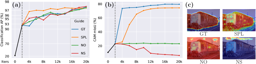
Figure 1: Oracle Experiments on VOC. CAMs are guided by the ground truth (GT), proposed segmentation pseudo-labels (SPL), no guidance (NO) and random noise (NS). (a): classification performance; (b): CAM quality; (c) CAMs visualization. All experiments employ 2k-iters warm-up before guidance is introduced.

To demonstrate this, we conduct oracle experiments in which we supervise the output CAMs from a classifier directly with the ground truth segmentation (GT). This enables all elements in $F$ to be optimized. For comparison, we conduct experiments wherein the CAMs are (i) not guided (NO), (ii) guided with masks of random noise (NS).

Results, shown in Fig. 1, demonstrate that different guidance for $M$ does not affect classification even for the NS group, as all experiment groups achieved over 97% classification precision. However, drastic differences can be observed w.r.t. the quality of the CAMs. The GT group results in a notable quality improvement over the NO group, as shown in Fig. 1(b)(c). In contrast, the NS group sabotages the CAMs. This suggests the stochasticity of CAMs and explains their variability and lack robustness, something also observed in [2, 60, 13].

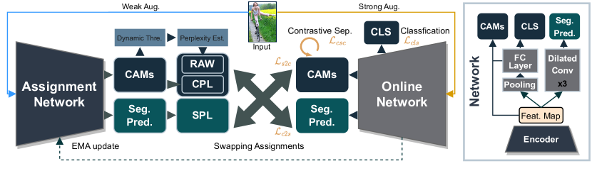
Figure 2: Co-training with Swapping Assignments (CoSA). We propose an end-to-end dual-stream weakly-supervised segmentation framework, capable of co-optimizing the segmentation prediction and CAMs by leveraging the swapped assignments, namely CAM pseudo-labels (CPL) and segmentation pseudo-labels (SPL). Our framework comprises two networks: an assignment network (AN) and an online network (ON), where the AN is responsible for generating pseudo-labels for training the ON. While the AN has identical architecture to the ON, it is updated through exponential moving average (EMA) of the ON. The diagram on the right provides an illustration of the architecture. Given weak-augmented images as input, the AN produces CPL to supervise segmentation in the ON ($\mathcal{L}_{\text{c2s}}$). During training, the CPL is softened by reliability-based adaptive weighting (RAW), formed based on CAM perplexity estimation and dynamic thresholding. The AN also generates SPL which is utilized to supervise the CAMs ($\mathcal{L}_{\text{s2c}}$). Further, the CAMs are regularized to contrastively separate the foreground from the background regions ($\mathcal{L}_{\text{csc}}$). Note that the ON is also trained for classification using the image-level class labels ($\mathcal{L}_{\text{cls}}$).

Since relying on GT segmentation is not feasible in WSSS, we propose an alternative for guiding CAMs, employing mask predictions as segmentation pseudo-labels (SPL). As shown in Fig. 1, an SPL-guided classifier yields CAMs that significantly outperform vanilla CAMs (NO group), performing close to the oracle trained with the GT. Motivated by this, we introduce a co-training mechanism in which CAMs and mask predictions are optimized mutually without any additional CAM refinement.

3.2 Co-training with Swapping Assignments

Overall Framework. As shown in Fig. 2, CoSA contains two networks: an online network (ON) and an assignment network (AN). ON, parameterized by $\Theta$, comprises three parts: a backbone encoder, FC layers, and a segmentation head. AN has the same architecture as ON but uses different weights, denoted $\Theta^{\prime}$. ON is trained with the pseudo assignments generated by AN, while AN is updated by the exponential moving average of ON: $\Theta^{\prime}\leftarrow m\Theta^{\prime}+(1-m)\Theta,$ where $m\in[0,1]$ denotes a momentum coefficient. Consequently, the weights of AN represent a delayed and more stable version of the weights of ON, which helps to yield a consistent and stabilized learning target [22].

An image and class label pair $(x,Y_{\text{gt}})$ is randomly sampled from a WSSS dataset $\mathcal{D}$. CoSA utilizes two augmented views $\mathcal{T}_{s}(x)$ and $\mathcal{T}_{w}(x)$ as input for ON and AN, respectively, representing strong and weak image transformations. During training, AN produces CAMs $\mathcal{M}^{\prime}$ and segmentation predictions $\mathcal{S}^{\prime}$. The CAM pseudo-labels (CPL) and segmentation pseudo-labels (SPL) are generated by $\mathcal{M}^{\prime}$ and $\mathcal{S}^{\prime}$ after filtering with respect to $Y_{\text{gt}}$. CPL and SPL are subsequently used as learning targets for supervising the segmentation predictions $\mathcal{S}$ and CAMs $\mathcal{M}$ from ON, respectively.

Swapping Assignments. Our objective is to co-optimize $\mathcal{S}$ and $\mathcal{M}$. A naive approach could enforce the learning objectives $\mathcal{S}\triangleq\mathcal{S}^{\prime}$ and $\mathcal{M}\triangleq\mathcal{M}^{\prime}$ as a knowledge distillation process [25], where AN and ON play the roles of teacher and student. However, this assumes availability of a pretrained teacher which is not possible in WSSS settings. Instead, we setup a swapped self-distillation with the objective:

$$\small\mathcal{L}_{\text{swap}}=\mathcal{L}_{\text{c2s}}(\mathcal{S},\mathcal{M}^{\prime})+\mathcal{L}_{\text{s2c}}(\mathcal{M},\mathcal{S}^{\prime})~{},\vspace{-5pt}$$ (2)

where $\mathcal{L}_{\text{c2s}}$ optimizes the segmentation performance given the CPL, and $\mathcal{L}_{\text{s2c}}$ considers the CAM quality with respect to SPL. Building on self-distillation [6, 48], we present this swapped self-distillation framework tailored to facilitate information exchange between the CAMs and segmentation.

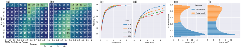
Figure 3: CPL Analysis on val splits of VOC (a, c, e) and COCO (b, d, f). (a) and (b): heatmap of CPL accuracy vs. confident ranges (x-axis) for different time-steps (y-axis). (c) and (d): correlation between perplexity and accuracy of CPL for different time-steps. (e) and (f): distribution of CAMs’ confidence categorized by the proposed dynamic threshold. (best viewed under zoom)

3.3 Segmentation Optimization.

CAM2Seg Learning. As the CAMs in CoSA are inherently guided, extra refinement [29, 2, 52] is not required, and they can be directly employed as learning targets. Nonetheless, CAMs primarily concentrate on the activated regions of the foreground while disregarding the background. As per the established convention [60, 15, 53], a threshold value $\xi$ is employed for splitting the foreground and the background. Formally, the CAM pseudo-label (CPL) is given by:

$$\small\hat{\mathcal{Y}}^{\text{CPL}}_{x,y}=\left\{\begin{aligned} &\mathtt{argmax}(\mathcal{M}_{x,y}^{\prime})+1,&\text{if $\nu\geq\xi$,}\\ &0,&\text{if $\nu<\xi$,}\\ \end{aligned}\right.,\vspace{-5pt}$$ (3)

where $\nu\triangleq\mathtt{max}(\mathcal{M}_{x,y}^{\prime})$ denotes the the maximum activation, $0$ denotes the background index. Then, the CAM2seg learning objective $\mathcal{L}_{\text{c2s}}$ is cross entropy between ${\mathcal{Y}}^{\text{CPL}}$ and $\mathcal{S}$, as with the general supervised segmentation loss [10].

Reliability based Adaptive Weighting. Segmentation performance depends heavily on the pseudo-labels. Despite the high-quality CPL generated by our guided CAMs, their reliability must be assessed, particularly in the initial training phases. Existing methods use post-refinement to increase reliability [70, 3]. As CoSA can generate online pseudo-labels, we propose to leverage confidence information to compensate the CAM2Seg loss during training.

Specifically, we propose to assess the perplexity scores for each pixel in $\hat{\mathcal{Y}}^{\text{CPL}}$ and leverage these scores to re-weight $\mathcal{L}_{\text{c2s}}$ for penalizing unreliable regions. However, estimating per-pixel perplexity is non-trivial. Through empirical analysis, we observe a noteworthy association between the confidence values of CAMs and their accuracy at each time-step. This correlation suggests that regions with extremely low or high confidence exhibit higher accuracy throughout training, as shown in Fig. 3(a)(b). To quantitatively model perplexity, we make two assumptions: i) the reliability of pseudo-labels is positively correlated with their accuracy, and ii) the perplexity score is negatively correlated with the reliability. Then, per-pixel perplexity of $\hat{\mathcal{Y}}^{\text{CPL}}_{x,y}$ is defined as:

$$\small\mathcal{P}_{x,y}=\left\{\begin{aligned} &\left[-\log\left(\lambda_{\alpha}(\nu-\xi)/(1-\xi)\right)\right]^{\lambda_{\beta}}&\text{if $\nu\geq\xi$,}\\ &\left[-\log\left(\lambda_{\alpha}(\xi-\nu)/\xi\right)\right]^{\lambda_{\beta}}&\text{if $\nu<\xi$,}\\ \end{aligned}\right.$$ (4)

where the term within the logarithm denotes the normalized distance to $\xi$ in $[0,1]$. The logarithm ensures $\mathcal{P}_{x,y}\!\rightarrow\!+\infty$ as distance $\!\rightarrow\!0$, and $\mathcal{P}_{x,y}\!\rightarrow\!0$ as distance $\rightarrow\!1$. $\lambda_{\alpha}\in\mathbb{R}^{+}$ controls the perplexity score’s minimum value and $\lambda_{\beta}\in\mathbb{R}^{+}$ determines the sharpness or smoothness of the distribution. Higher $\mathcal{P}_{x,y}$ indicates confidence of $\hat{\mathcal{Y}}^{\text{CPL}}_{x,y}$ closer to threshold $\xi$. This observation is substantiated by Fig. 3 (a)(b), where confidence values near $\xi\!=\!0.5$ exhibit lower reliability. Furthermore, the correlation between perplexity and accuracy remains significant across various training time-steps and datasets, as depicted in Fig. 3(c)(d).

Since we hypothesize negative reliability-perplexity correlation, the reliability score can be defined as the reciprocal of perplexity. To accommodate reliability variation for different input, we use the normalized reliability as the per-pixel weights for $\mathcal{L}_{\text{c2s}}$. Thus, Reliability based Adaptive Weighting (RAW) is defined as: $\mathcal{W}_{x,y}^{\text{raw}}=|\mathcal{R}|/\sum_{i,j\in\mathcal{R}}{(\mathcal{P}_{i,j}\mathcal{P}_{x,y})}^{-1}$, where $|\mathcal{R}|$ represents total number of pixels in a batch. Then, the re-weighted CAM2seg loss for each position $(x,y)$ can be defined as

$$\small\mathcal{L}_{\text{c2s}}(x,y)\!\!=\!\!-\mathcal{W}_{x,y}^{\text{raw}}\!\sum_{c=0}^{C}\!\Bigg{[}\!\mathbbm{1}\!\big{[}\hat{\mathcal{Y}}^{\text{CPL}}_{x,y}\!\!=\!\!c\big{]}\!\!\log\!\!\Bigg{(}\!\frac{\exp{\mathcal{S}^{c}_{x,y}}}{\sum_{k=0}^{C}\exp\mathcal{S}^{k}_{x,y}}\!\!\Bigg{)}\!\!\Bigg{]}.$$ (5)

Dynamic Threshold. Existing WSSS work [52, 53] prescribes a fixed threshold to separate foreground and background, which neglects inherent variability due to prediction confidence fluctuation during training. Obviously, applying a fixed threshold in Fig. 3(a)(b) is sub-optimal. To alleviate this, we introduce dynamic thresholding. As shown in Fig. 3(e)(f), the confidence distribution reveals discernible clusters. We assume the foreground and background pixels satisfy a bimodal Gaussian Mixture distribution. Then, the optimal dynamic threshold $\xi^{\star}$ is determined by maximizing the Gaussian Mixture likelihood:

$$\xi^{\star}=\underset{\xi}{\mathtt{argmax}} \prod_{x\in\{\mathcal{M}^{\prime}\geq\xi\}}\tilde{\pi}_{fg}\mathcal{N}\left(x\mid\tilde{\mu}_{fg},\tilde{\Sigma}_{fg}\right)$$ (6)

$$+ \prod_{x\in\{\mathcal{M}^{\prime}<\xi\}}\tilde{\pi}_{bg}\mathcal{N}\left(x\mid\tilde{\mu}_{bg},\tilde{\Sigma}_{bg}\right)~{},$$

where $\mathcal{N}(x\mid\mu,\Sigma)$ denotes the Gaussian function and $\pi$, $\mu$, $\Sigma$ represent the weight, mean and covariance. To avoid mini-batch bias, we maintain a queue to fit GMM, with the current $\mathcal{M}^{\prime}$ batch enqueued and the oldest dequeued. This practice facilitates the establishment of a gradually evolving threshold, contributing to learning stabilization.

3.4 CAM Optimization.

Seg2CAM Learning. To generate SPL, segmentation predictions $\mathcal{S}^{\prime}$ are filtered by the weak labels $Y_{\text{gt}}$ and transformed into probabilities:

$$\small\mathcal{S}^{\prime~{}c}_{x,y}=\left\{\begin{aligned} &-\infty,\!\!\!&\text{if $Y_{\text{gt}}^{c}=0$,}\\ &\mathcal{S}^{\prime~{}c}_{x,y},\!\!\!&\text{if $Y_{\text{gt}}^{c}\neq 0$,}\\ \end{aligned}\right.\;\;\;\;\hat{\mathcal{Y}}^{\text{SPL}}_{x,y}=\mathtt{Softmax}(\frac{\mathcal{S}^{\prime}_{x,y}}{\tau})~{},\vspace{-5pt}$$ (7)

where $\tau$ represents the softmax temperature to sharpen the $\hat{\mathcal{Y}}^{\text{SPL}}$. Then, we arrive Seg2CAM learning objective:

$$\mathcal{L}_{\text{s2c}}=-\frac{1}{C|\mathcal{R}|} \sum_{c=1}^{C}\sum_{x,y\in\mathcal{R}}\bigg{[}\hat{\mathcal{Y}}^{\text{SPL}}_{x,y}[c]\log(\sigma(\mathcal{M}^{c}_{x,y}))$$ (8)

$$+ (1-\hat{\mathcal{Y}}^{\text{SPL}}_{x,y}[c])\log(1-\sigma(\mathcal{M}^{c}_{x,y}))\bigg{]}~{},$$

where $\mathcal{R}$ represents all the positions in SPL.

Coexistence Problem in CAMs. Certain class activations often exhibit large false positive regions, where objects are incorrectly merged with surroundings, as shown in Fig. 8 (1st row). For instance, the classes ’bird’ and ’tree branches’, ’train’ and ’railways’, etc. frequently appear together in VOC. We refer to this issue as the coexistence problem. We hypothesize that the coexistence problem is attributed to three factors: i) Objects that coexist in images, such as ’tree branches’, are not annotated w.r.t. weak labels, which makes it challenging for a model to semantically distinguish coexistence. ii) Training datasets lack sufficient samples for such classes. iii) High-level feature maps, though rich in abstract representations and semantic information, lack essential low-level features such as edges, textures, and colors [24]. Thus, CAMs generated from the last layer are poor in low-level information for segmenting objects. Conversely, segmenting objects with high-level semantics is hindered due to factors i) and ii).

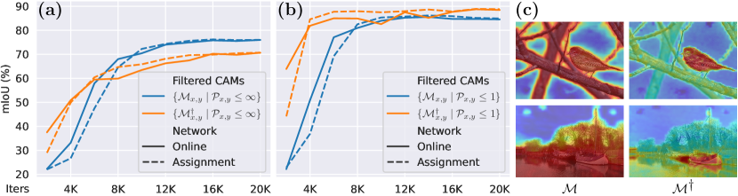
Figure 4: $\mathcal{M}$ and $\mathcal{M}^{\dagger}$ Comparisons. (a): mIoU vs. time-steps for $\mathcal{M}$ and $\mathcal{M}^{\dagger}$ on VOC val. (b): same as (a) but filtered by perplexity. (c): cases of coexistence issue in $\mathcal{M}$ but not in $\mathcal{M}^{\dagger}$.

Contrastive Separation in CAMs. We posit that the effective usage of low-level information can alleviate the coexistence problem. Since shallower-layer feature maps contain more low-level information, we propose to extract CAMs from earlier in the backbone, denoted $\mathcal{M}^{\dagger}$, and present a comparison with $\mathcal{M}$ in Fig. 4, showing that substituting $\mathcal{M}$ with $\mathcal{M}^{\dagger}$ is not feasible due to the lower mIoU upperbound of $\mathcal{M}^{\dagger}$. If we consider the confident regions in $\mathcal{M}$ and $\mathcal{M}^{\dagger}$, i.e. filter by a low-pass perplexity $\mathcal{P}$, $\{\mathcal{M}^{\dagger}_{x,y}\!\mid\!\mathcal{P}_{x,y}\!\leq\!\epsilon\}$ are better than $\{\mathcal{M}_{x,y}\!\mid\!\mathcal{P}_{x,y}\!\leq\!\epsilon\}$, as shown in Fig. 4(b), where $\epsilon$ represents a low-pass coefficient. Fig. 4(c) illustrates the presence of coexistence issues in $\mathcal{M}$ but absence in $\mathcal{M}^{\dagger}$. Those findings suggest that $\mathcal{M}^{\dagger}$ is worse than $\mathcal{M}$ in general, but better for those regions with low perplexity.

In CoSA, we propose to regularize $\mathcal{M}$ by $\mathcal{M}^{\dagger\prime}$ (from AN). We define positive $\mathcal{R}^{+}_{i,j}$ and negative $\mathcal{R}^{-}_{i,j}$ regions as

$$\mathcal{R}^{+}_{i,j} =\Big{\{}(x,y)\mid\mathcal{P}_{x,y}\leq\epsilon,~{}\hat{y}^{\text{CPL}}_{x,y}=\hat{y}^{\text{CPL}}_{i,j},(x,y)\neq(i,j)\Big{\}}$$ (9)

$$\mathcal{R}^{-}_{i,j} =\Big{\{}(x,y)\mid\mathcal{P}_{x,y}\leq\epsilon,~{}\hat{y}^{\text{CPL}}_{x,y}\neq\hat{y}^{\text{CPL}}_{i,j}\Big{\}}~{},$$

where $(i,j)\!\in\!\Omega$, $\Omega\!=\!\{(x,y)\!\mid\!\mathcal{P}_{x,y}\!\leq\!\epsilon\}$ is low-perplexity region in $\mathcal{M}^{\dagger\prime}$, and $\hat{y}^{\text{CPL}}$ represents the CPL of $\mathcal{M}^{\dagger\prime}$. Then, we arrive the contrastive separation loss for $\mathcal{M}$:

$$\small\mathcal{L}_{\text{csc}}=-\frac{1}{\lvert\Omega\rvert}\sum_{i,j\in\Omega}\frac{1}{\lvert\mathcal{R}^{+}_{i,j}\rvert}\sum_{x,y\in\mathcal{R}^{+}_{i,j}}\log\frac{L_{x,y}^{i,j}}{L_{x,y}^{i,j}+K_{n,m}^{i,j}}~{},$$ (10)

where $L_{x,y}^{i,j}\!=\!\exp(l_{d}(\mathcal{M}_{i,j},\mathcal{M}_{x,y})/\tau)$, $l_{d}(a,b)$ measures the (a,b) distance, $\tau$ denotes the InfoNCE loss [47] temperature, and $K_{n,m}^{i,j}\!=\!\sum_{n,m\in\mathcal{R}^{-}_{i,j}}L_{n,m}^{i,j}$.

Overall Objectives. The objectives encompass the aforementioned losses and a further $\mathcal{L}_{\text{c2s}}^{\mathcal{M}^{\dagger}}$ to stabilize training and accelerate convergence, resulting in the CoSA objective:

$$\small\mathcal{L}_{\text{CoSA}}\!\!=\!\mathcal{L}_{\text{cls}}\!+\mathcal{L}_{\text{cls}}^{\mathcal{M}^{\dagger}}\!\!+\!\lambda_{\text{c2s}}\big{(}\mathcal{L}_{\text{c2s}}\!+\!\mathcal{L}_{\text{c2s}}^{\mathcal{M}^{\dagger}}\big{)}\!+\!\lambda_{\text{s2c}}\mathcal{L}_{\text{s2c}}+\!\lambda_{\text{csc}}\mathcal{L}_{\text{csc}}.$$ (11)

4 Experiments

4.1 Experiment Details and Results

Datasets. We evaluate on two benchmarks: PASCAL VOC 2012 [19] and MS-COCO 2014 [41]. VOC encompasses 20 categories with train, val, and test splits of 1464, 1449, and 1456 images. Following WSSS practice [2, 3, 65], SBD [23] is used to augment the train split to 10,582. COCO contains 80 categories with train and val splits of approx. 82K and 40K images. Our model is trained and evaluated using only the image-level classification labels, and employing mIoU as evaluation metrics.

Implementation Details. Following [53], we use ImageNet pretrained ViT-base (ViT-B) [17] as the encoder. For classification, we use global max pooling (GMP) [51] and the CAM approach [72]. For the segmentation decoder, we use LargeFOV [10], as with [53]. ON is trained with AdamW [46]. The learning rate is set to 6E-5 in tandem with polynomial decay. AN is updated with a momentum of $0.9994$. For preprocessing, the images are cropped to $448^{2}$, then weak/strong augmentations are applied (see Supp. Materials). The perplexity constants $(\lambda_{\alpha},\lambda_{\beta})$ are set to $(0.8,1)$, GMM-fitting queue length is $100$, and softmax temperature $\tau$ is $0.01$. The low perplexity threshold $\epsilon$ is set to $1$ and the loss weight factors $(\lambda_{\text{c2s}},\lambda_{\text{s2c}},\lambda_{\text{csc}})$ to $(0.1,0.05,0.1)$.

Method	Backbone	train	val
RRM [70] AAAI’2020	WR38	–	65.4
1Stage [3] CVPR’2020	WR38	66.9	65.3
AFA [52] CVPR’2022	MiT-B1	68.7	66.5
MCT [65] CVPR’2022	MCT	69.1	–
ViT-PCM [51] ECCV’2022	ViT-B	71.4	69.3
Xu et al. [66] CVPR’2023	ViT-B	66.3	–
ACR-ViT [31] CVPR’2023	ViT-B	70.9	–
CLIP-ES [42] CVPR’2023	ViT-B	75.0	–
ToCo [53] CVPR’2023	ViT-B	73.6	72.3
CoSA	ViT-B	78.5	76.4
CoSA∙	ViT-B	78.9	77.2

Table 1: Comparisons of CPL. CAM pseudo-labels evaulation on VOC dataset. Backbone denotes the encoder used for generating the CAMs. $\bullet$ represents the ensemble of $\mathcal{M}^{\prime}$ and $\mathcal{M}^{\dagger\prime}$ in CoSA.

Methods	Sup.	Net.	VOC		COCO
			val	test	val
Supervised Upperbounds.
Deeplab [10] TPAMI’2017	$\mathcal{F}$	R101	77.6	79.7	–
WideRes38 [61] PR’2019	$\mathcal{F}$	WR38	80.8	82.5	–
ViT-Base [17] ICLR’2021	$\mathcal{F}$	ViT-B	80.5	81.0	–
UperNet-Swin [44] ICCV’2021	$\mathcal{F}$	SWIN	83.4	83.7	–
Multi-stage Methods.
L2G [26] CVPR’2022	$\mathcal{I}+\mathcal{S}$	R101	72.1	71.7	44.2
Du et al. [18] CVPR’2022	$\mathcal{I}+\mathcal{S}$	R101	72.6	73.6	–
CLIP-ES [42] CVPR’2023	$\mathcal{I}+\mathcal{L}$	R101	73.8	73.9	45.4
ESOL [39] NeurIPS’2022	$\mathcal{I}$	R101	69.9	69.3	42.6
BECO [50] CVPR’2023	$\mathcal{I}$	R101	72.1	71.8	45.1
Mat-Label [59] ICCV’2023	$\mathcal{I}$	R101	73.0	72.7	45.6
CoSA-MS	$\mathcal{I}$	R101	76.5	75.3[1]	50.9
Xu et al. [66] CVPR’2023	$\mathcal{I}+\mathcal{L}$	WR38	72.2	72.2	45.9
W-OoD [35] CVPR’2022	$\mathcal{I}$	WR38	70.7	70.1	–
MCT [65] CVPR’2022	$\mathcal{I}$	WR38	71.9	71.6	42.0
ex-ViT [69] PR’2023	$\mathcal{I}$	WR38	71.2	71.1	42.9
ACR-ViT [31] CVPR’2023	$\mathcal{I}$	WR38	72.4	72.4	–
MCT+OCR [15] CVPR’2023	$\mathcal{I}$	WR38	72.7	72.0	42.0
CoSA-MS	$\mathcal{I}$	WR38	76.6	74.9[2]	50.1
ReCAM [14] CVPR’2022	$\mathcal{I}$	SWIN	70.4	71.7	47.9
LPCAM [12] CVPR’2023	$\mathcal{I}$	SWIN	73.1	73.4	48.3
CoSA-MS	$\mathcal{I}$	SWIN	81.4	78.4[3]	53.7
Single-stage (End-to-end) Methods.
1Stage [3] CVPR’2020	$\mathcal{I}$	WR38	62.7	64.3	–
RRM [70] AAAI’2020	$\mathcal{I}$	WR38	62.6	62.9	–
AFA [52] CVPR’2022	$\mathcal{I}$	MiT-B1	66.0	66.3	38.9
RRM [70]† AAAI’2020	$\mathcal{I}$	ViT-B	63.1	62.4	–
ViT-PCM [51] ECCV’2022	$\mathcal{I}$	ViT-B	69.3	–	45.0
ToCo [53] CVPR’2023	$\mathcal{I}$	ViT-B	71.1	72.2	42.3
CoSA	$\mathcal{I}$	ViT-B	76.2	75.1[4]	51.0
CoSA∗	$\mathcal{I}$	ViT-B	76.4	75.2[5]	51.1

Table 2: Weakly Supervised Semantic Segmentation Results. Sup.: supervision type. Net.: segmentation backbone. $\mathcal{F}$: Fully supervised, $\mathcal{I}$: Image-level labels, $\mathcal{S}$: Saliency maps, $\mathcal{L}$: language models. $*$ represents CRF [10] postprocessing results.

CAM Quality Comparison. Tab. 1 shows CoSA CPL results on VOC compared with existing WSSS methods, using our $\hat{\mathcal{Y}}^{\text{CPL}}$ ($\xi\!\!=\!\!0.5$). Our method yields 78.5% and 76.4% mIoU on train and val. Notably, an ensemble of $\mathcal{M}^{\prime}$ and $\mathcal{M}^{\dagger\prime}$ improves performance to 78.9% and 77.2%, suggesting the activation of $\mathcal{M}^{\prime}$ is orthogonal to that of $\mathcal{M}^{\dagger\prime}$.

Semantic Segmentation Comparison. We compare our method with existing SOTA WSSS methods on VOC and COCO for semantic segmentation in Tab. 2. CoSA achieves 76.2% and 75.1% on VOC12 val and test, respectively, surpassing the highest-performing single-stage model (ToCo) by 5.1% and 2.9%, as well as all multi-stage methods, including those with additional supervision. In the COCO evaluation, CoSA consistently outperforms other approaches, demonstrating a significant increase of 8.7% over the top-performing single-stage methods. Further, there is a also 2.7% improvement over the leading multi-stage method [12]. While our primary goal is to provide an end-to-end WSSS solution, we also offer a multi-stage version of CoSA, denoted as CoSA-MS in Tab. 2, where various standalone segmentation networks are trained using our CPL. Our CoSA-MS models can also attains SOTA performance in multi-stage scenarios.

Qualitative Comparison. Fig. 5 presents CAMs and segmentation visualizations, comparing with recent methods: MCT, BECO, and ToCo. As shown, our method can generate improved CAMs and produce well-aligned segmentation, exhibiting superior results in challenging segmentation problems with intra-class variation and occlusions. In addition, CoSA performs well w.r.t. the coexistence cases (Fig. 5 R1, R2), while existing methods struggle. Moreover, CoSA reveals limitations in the GT segmentation (Fig. 5 R4).

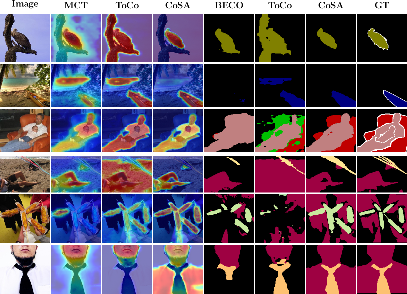
Figure 5: Qualitative Comparison. The results are reported on the val splits of VOC (in R1 - R3) and COCO (in R4 - R6). The official codebases and provided weights for MCT [65], BECO [50], and ToCo [53] are used for this comparison. (best viewed under zoom; see Supp. Materials for more high-res Comparisons).

4.2 Ablation Studies

CoSA Module Analysis. We begin by employing CAMs directly as the supervision signal for segmentation, akin to [70], albeit without refinement, and gradually apply CoSA modules to this baseline. As shown in Tab. 3(a), the mIoUs progressively improve with addition of our components. Further, we examine the efficacy of each CoSA component. As shown in Tab. 3(b), the elimination of each component results in deteriorated performance, most notably for CSC.

(a)
mIoU (inc.) Base. GC SA RAW CSC DT VOC COCO ✓ 55.96 37.32 ✓ ✓ 63.09 (+7.13) 42.55 (+5.23) ✓ ✓ ✓ 64.41 (+8.45) 43.92 (+6.60) ✓ ✓ ✓ ✓ 68.22 (+12.26) 45.39 (+8.07) ✓ ✓ ✓ ✓ 71.66 (+15.70) 47.10 (+9.78) ✓ ✓ ✓ ✓ ✓ 75.54 (+19.58) 49.67 (+12.35) ✓ ✓ ✓ ✓ ✓ ✓ 76.19 (+20.23) 51.00 (+13.68)

(b)
mIoU (dec.) CoSA GC SA RAW CSC DT VOC COCO ✓ 76.19 51.00 ✓ ✗ 75.54 (-0.65) 49.67 (-1.33) ✓ ✗ 69.89 (-6.30) 45.95 (-5.05) ✓ ✗ 72.45 (-3.74) 47.83 (-3.17) ✓ ✗ 72.10 (-4.09) 49.04 (-1.96) ✓ ✗ 74.12 (-2.07) 49.67 (-1.33)

Table 3: Ablation Study on Contribution of Each Component. (a): gradually add proposed components to baseline. (b): systematically exclude components from CoSA. GC: Guided CAMs, SA: Swapping Assignments, RAW: Reliability based Adaptive Weighting, CSC: Contrastive Separation in CAMs, and DT: Dynamic Threshold. mIoU is reported on PASCAL VOC12 and COCO val splits.

(a) Source Detach train val GT None 83.99 80.16 NO – 72.28 71.38 SPL $F$ 74.19 73.36 SPL $W_{\text{fc}}$ 78.05 76.15 SPL None 78.54 76.37

(b) Method C-mIoU mIoU FPR [8] 53.09 53.34 MCT [65] 58.46 61.24 ToCo [53] 63.62 72.33 w/o CSC 62.61 67.82 w/ CSC 82.34 76.37

Table 4: Ablation Study of GC & CSC. (a): CPL performance comparison on VOC for CAMs. Detach: stop gradient in GC for feature map $F$ or FC weights $W_{\text{fc}}$. Source: guidance sources. (b): CPL performance comparison on VOC. FPR, MCT and ToCo results are based on provided code and weights. C-mIoU: mIoU for classes with coexistence issues.

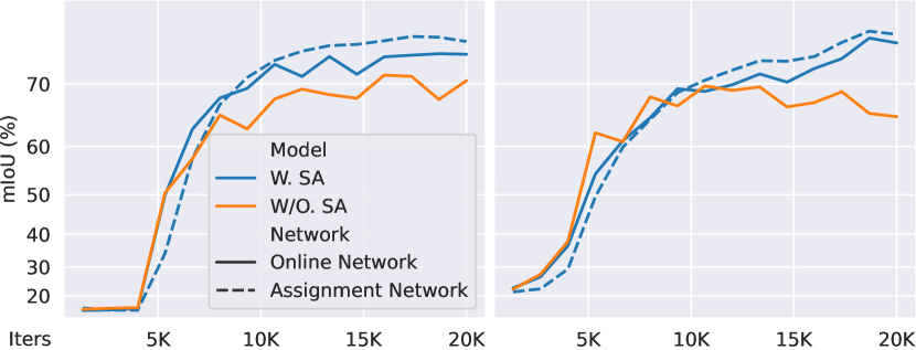
Figure 6: Ablative Study of SA. The performance of SPL (left) and CPL (right) w.r.t. iterations on VOC val set are shown for CoSA with or without SA.

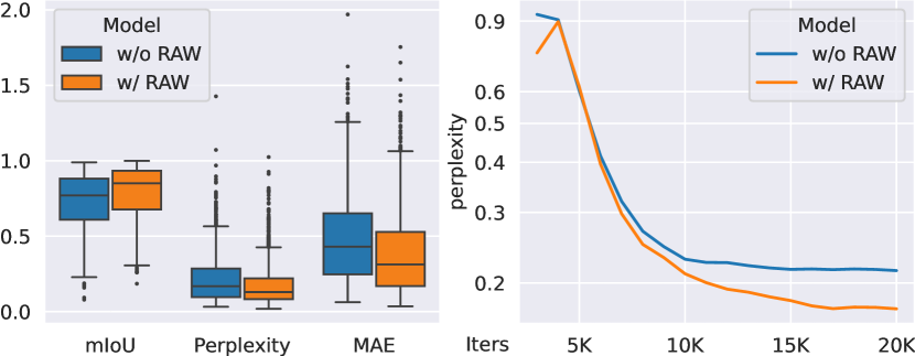
Figure 7: Ablation Study of RAW. (left) boxplot of mIoU, perplexity and MAE to (1,0) for individual CPLs on VOC val. (right) perplexity reduction over times.

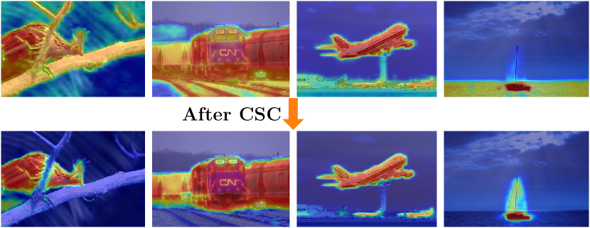
Figure 8: Coexistence Problems & Effect of CSC. The class activation for bird, train, airplane, and boat are presented from left to right. (best viewed under zoom)

Impact of Guided CAMs. We evaluate the impact of including guided CAMs w.r.t. CAM quality, comparing a baseline using vanilla CAMs [72] as CPL following [70, 52] with the proposed guided CAMs. As shown in Tab. 4(a), our guided CAMs notably enhance CPL quality by 6.26% and 4.99% for train and val splits. Further, we conduct experiments to ascertain the extent to which the two CAM components, feature map $F$ and classification weights $W_{\text{fc}}$, exert greater impact on guiding CAMs. As shown, disconnection of $F$ from the gradient chains results in 74.19% and 73.36%, while the detachment of $W_{\text{fc}}$ decrease the results slightly to 78.05% and 76.37%. This suggests that guiding CAMs primarily optimizes the feature maps, verifying our initial hypothesis of the inherent non-deterministic feature map contributing to the stochasticity of CAMs in Sec. 3.1.

Impact of Swapping Assignments (SA). Tab. 3(b) suggests that eliminating SA results in significant mIoU decreases, highlighting the importance of this training strategy. Further examination of the ON and AN w.r.t. SPL and CPL indicates that, in later training stages, AN consistently outperforms ON for both SPL and CPL, as shown in Fig. 8, due to AN performing a form of model ensembling similar to Polyak-Ruppert averaging [49, 54]. We observe a noticeable disparity of mIoUs between two ONs (solid orange line vs. solid blue line in Fig. 8), which may be attributed to the superior quality of CPL and SPL from the AN facilitating a more robust ON for CoSA. The momentum framework, originally introduced to mitigate noise and fluctuations of the online learning target [22, 6], is used for information exchange across CAMs and segmentation in CoSA. To the best of our knowledge, we are the first to apply and demonstrate the efficacy of this type of training scheme in WSSS.

Impact of RAW. Tab. 3(b) shows notable mIoU reduction without RAW. We conduct further studies to investigate its effect on perplexity reduction. The boxplot in Fig. 8 suggests that RAW leads to higher mIoU but lower perplexity. Fig. 8(right) illustrates a faster decrease in perplexity when RAW is used, affirming its impact on perplexity reduction.

Impact of CSC. Our CSC is introduced to address the coexistence issue. We establish C-mIoU to measure the CAM quality for those coexistence-affected classes. As shown in Tab. 4(b), applying CSC sees a boost in C-mIoU and mIoU, which surpass the existing methods. Some visual examples demonstrating these enhancements are given in Fig. 8.

Impact of Dynamic Threshold. We evaluate CoSA using some predetermined thresholds, comparing them with one employing dynamic threshold on VOC val split (see Supp. Materials for results). The performance is sensitive to the threshold, but dynamic thresholding achieves 0.65% increased performance over the best manual finetuning while saving 80% of hyper-parameter searching time.

5 Conclusion

This paper presents an end-to-end WSSS method: Co-training with Swapping Assignments (CoSA), which eliminates the need for CAM refinement and enables concurrent CAM and segmentation optimization. Our empirical study reveals the non-deterministic behaviors of CAMs and that proper guidance can mitigate such stochasticity, leading to substantial quality enhancement. We propose explicit CAM optimization leveraging segmentation pseudo-labels in our approach, where a dual-stream model comprising an online network for predicting CAMs and segmentation masks, and an ancillary assignment network providing swapped assignments (SPL and CPL) for training, is introduced. We further propose three techniques within this framework: RAW, designed to mitigate the issue of unreliable pseudo-labels; contrastive separation, aimed at resolving coexistence problems; and a dynamic threshold search algorithm. Incorporating these techniques, CoSA outperforms all SOTA methods on both VOC and COCO WSSS benchmarks while achieving exceptional speed-accuracy trade-off.

Appendix A Additional Results

A.1 Hyper-parameter Finetuning

Here, we examine the impact of hyper-parameter variation with CoSA resulting from our finetuning. The fine-tuning of each hyper-parameter is demonstrate with the remaining parameters fixed at their determined optimal values.

Loss Weights. We demonstrate the finetuning of the Seg2CAM and CAM2Seg loss weights in Tab. 5(a)(b). A significant mIoU decrease is observed as $\lambda_{c2s}$ reduces the influence of the segmentation branch, as expected. The mIoU reaches its peak when $\lambda_{\text{s2c}}\!=\!0.05$ and $\lambda_{\text{c2s}}\!=\!0.1$.

Low-perplexity Filter. We finetune the coefficient for the low-pass perplexity filter $\epsilon$, described in eq. (9) of the main paper. The corresponding findings are illustrated in Tab. 5(c). Optimum performance is obtained when $\epsilon$ is set to $1$, either decreasing or increasing this value can impair the performance of our model.

EMA Momentum. Here, the momentum used for updating the assignment network is finetuned. Results presented in Tab. 5(d) indicate that the optimal performance is achieved when $m=0.9994$. Additionally, we find that setting $m=1$ freezes the assignment network, breaking the training of online network and leading to framework collapse.

Fixed Threshold vs. Dynamic Threshold. In this study, we evaluate CoSA with predetermined thresholds. The results are presented in Fig. 9. As shown, the performance peaks when this threshold is set to $0.45$, with an mIoU of $75.54\%$. However, our dynamic threshold can outperform the best manual finetuning by $0.65\%$. Despite the incurred additional $10\%$ computation overhead, our threshold searching algorithm obviates time-consuming finetuning efforts, resulting in nearly 80% reduction in hyper-parameter searching time in this case and $(1-1.1n^{-1})\%$ in general where $n$ thresholds are considered. In addition, the adoption of dynamic thresholding can enhance the generalizability to novel datasets.

(a) Seg2CAM weight $\lambda_{\text{s2c}}$

$\lambda_{\text{s2c}}$	mIoU
$0.2$	73.79
$0.1$	74.67
$0.05$	76.19
$0.025$	75.25
$0.0125$	74.33

(b) CAM2Seg weight $\lambda_{\text{c2s}}$

$\lambda_{\text{c2s}}$	mIoU
$0.4$	74.67
$0.2$	75.56
$0.1$	76.19
$0.05$	73.95
$0.025$	61.55

(c) Perplexity filter $\epsilon$

$\epsilon$	mIoU
$\infty$	73.66
$2$	75.52
$1$	76.19
$0.5$	74.30
$0.1$	70.63

(d) Momentum $m$

$m$	mIoU
$0.9990$	73.79
$0.9992$	75.40
$0.9994$	76.19
$0.9996$	75.58
$0.9999$	71.42
$1.0000$	15.99

Table 5: Hyper-parameters Finetuning Results. Parameter searching for (a) Loss weight for CAM2Seg $\lambda_{\text{c2s}}$; (b) Loss weight for Seg2CAM $\lambda_{\text{s2c}}$; (c) Low-pass perplexity filter coefficient $\epsilon$; (e) EMA Momentum $m$ for updating assignment network. mIoU represents semantic segmentation result on PASCAL VOC val split.

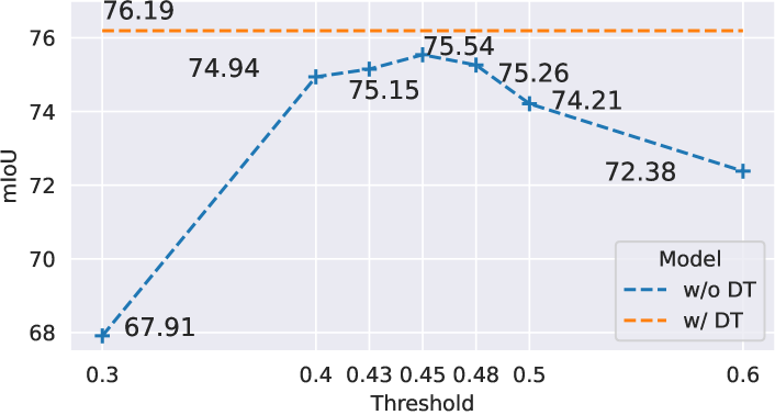
Figure 9: Threshold finetuning. (left) determined dynamic threshold during training. (right) mIoU comparison of fixed threshold vs. the purposed dynamic threshold on VOC val.

A.2 Per-class Segmentation Comparisons

We show the per-class semantic segmentation results on VOC val and test splits as well as COCO val split.

Comparisons on VOC. Tab. 12 illustrates the CoSA per-class mIoU results compared with recent works: AdvCAM [33], MCT [65], ToCo [53], Xu et al. [66], BECO [50]. To be fair in comparison, we include CoSA with CRF [10] postprocessing results, denoted as CoSA^∗, same as other SOTA models. Notably, CoSA dominates in 10 out of 21 classes. In particular, categories like boat ($5.9\%\!\uparrow$), chair ($8.2\%\!\uparrow$), and sofa ($17.2\%\!\uparrow$), demonstrate substantial lead over the SOTA models. In the VOC test split (depicted in Tab. 12), we still observe its superiority over other SOTA methods, where CoSA dominates in 15 out of 21 classes.

Comparisons on COCO. We compare CoSA with recent WSSS works for individual class performance on the COCO val set. As illustrated in Tab. 13, CoSA outperforms its counterparts in 56 out of 81 classes. Particularly, classes such as truck ($10.6\%\!\uparrow$), tie ($14.3\%\!\uparrow$), kite ($12.4\%\!\uparrow$), baseball glove ($20.3\%\!\uparrow$), knife ($14.5\%\!\uparrow$), ($10.6\%\!\uparrow$), carrot ($13.0\%\!\uparrow$), donuts ($10.0\%\!\uparrow$), couch ($13.9\%\!\uparrow$), oven ($13.0\%\!\uparrow$), and toothbrush ($10.0\%\!\uparrow$) exhibit remarkable leading performance.

A.3 Further Qualitative Comparisons

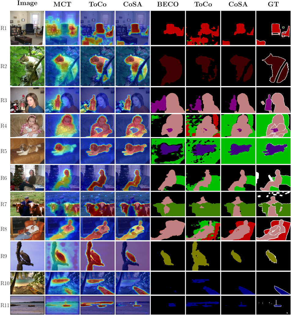
Figure 10: Qualitative Comparisons on VOC Dataset. CoSA exhibits 1) better foreground-background separation (R1–R3); 2) more robust to inter-class variation and occlusion (R4–R7); 3) limitations in the ground troth annotations (R8); 4) less coexistence problem (R9–R11). Different colors represent different categories: black: background; white: ignore areas; : chair; : plant; : cat; : person; : bottle; : sofa; : dog; : cow. : bird; : boat; The activated classes in the demonstration from top to bottom are: chair, cat, bottle, person, dog, person, cow, person, bird, boat, boat.

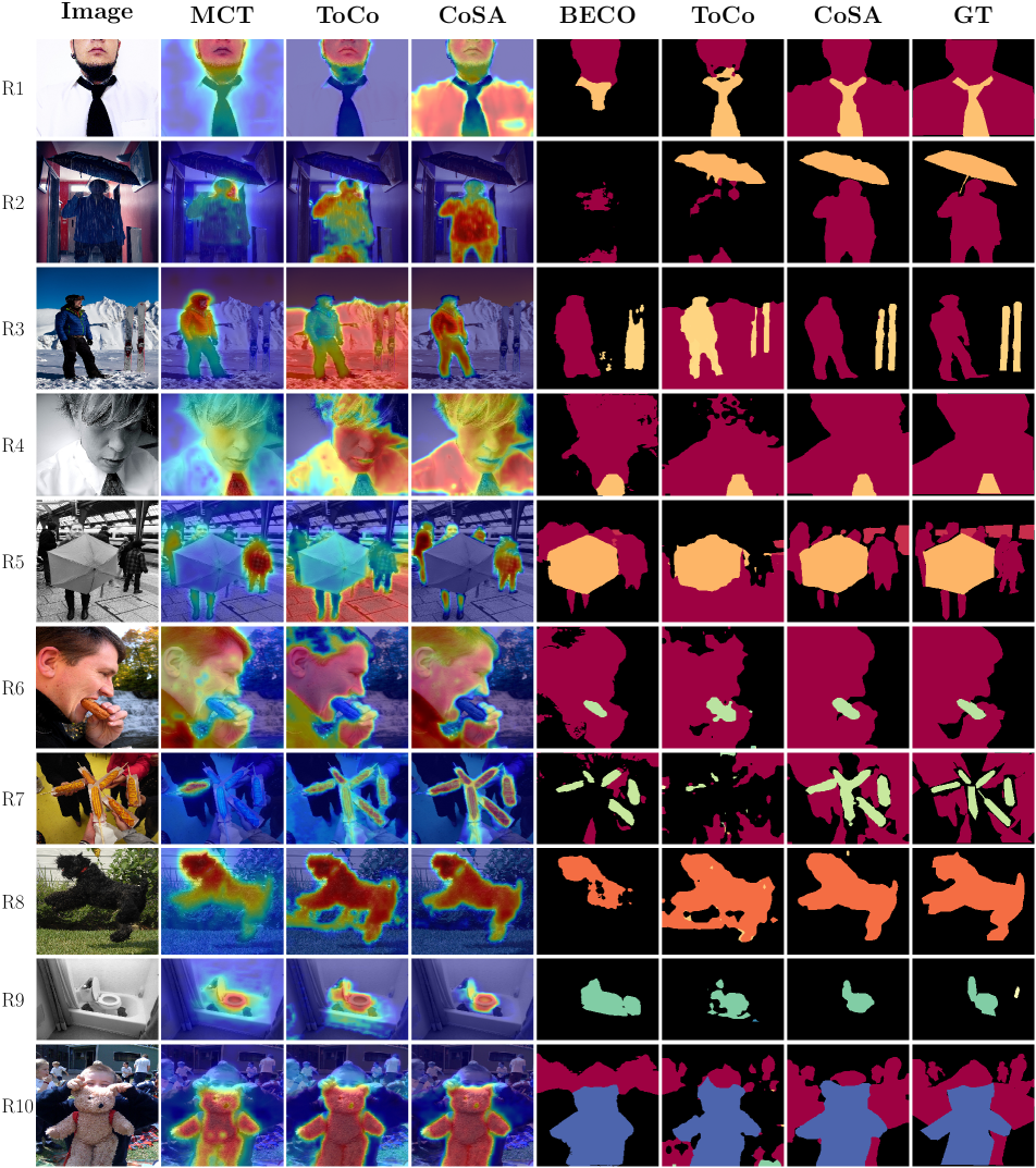
Figure 11: Qualitative Comparisons on COCO Dataset. CoSA demonstrates superior quality in terms of foreground-background separation (R1–R10). Categories involved – R1: person, tie; R2: person, umbrella; R3: person, skis; R4: person, tie; R5: person, train, umbrella; R6: person, hot dog; R7: person, hot dog; R8: dog, frisbee; R9: bottle, toilet; R10: person, teddy bear; Categories in Bold denotes the activated classes in CAMs.

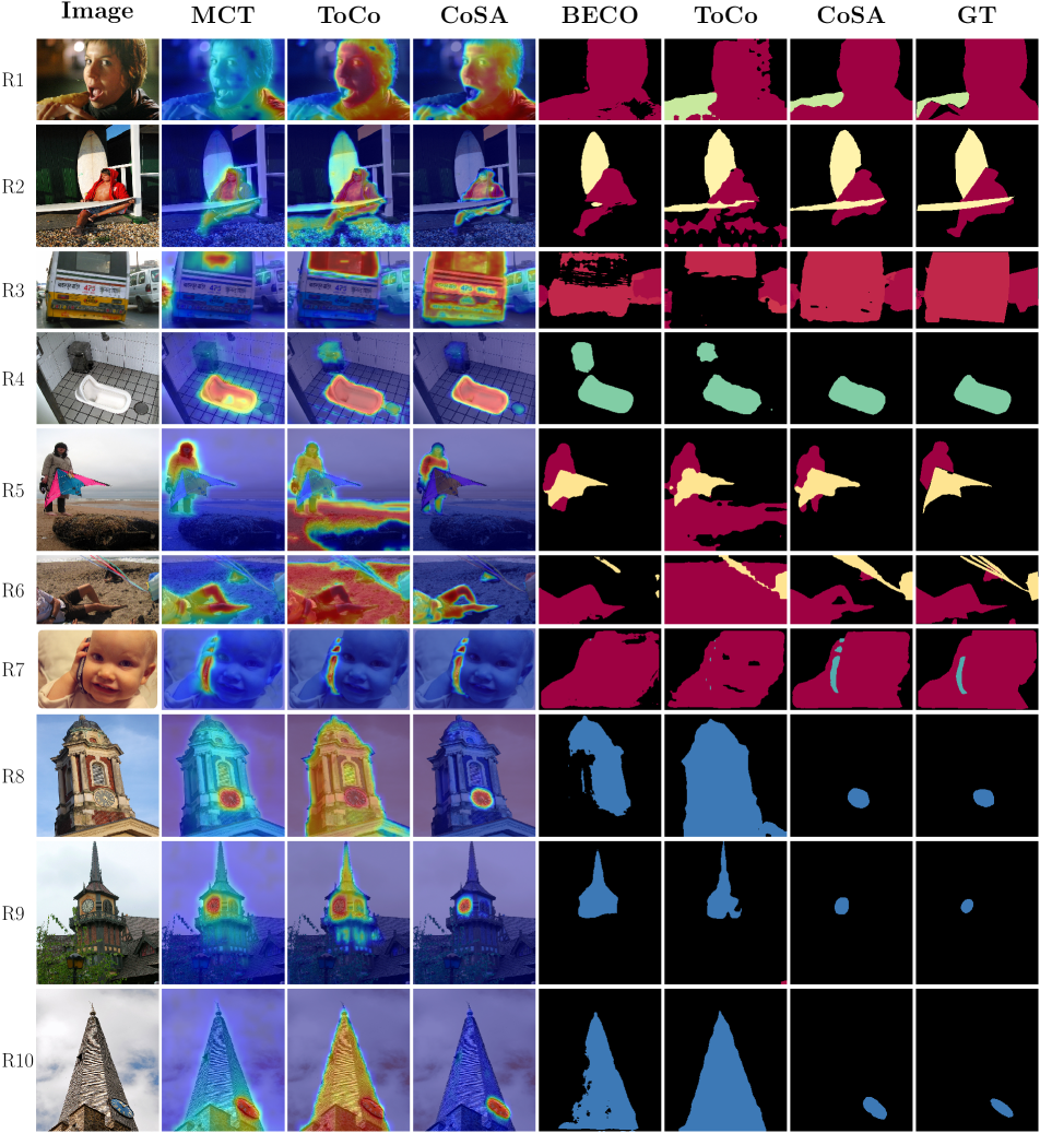
Figure 12: More Qualitative Comparisons on COCO Dataset. CoSA shows 1) more robust to inter-class variation and occlusion (R1–R4); 2) limitations in the ground troth annotations (R5–R7); 3) less coexistence problem (R8–R10). Categories involved – R1: person, donuts; R2: person, surfboard. R3: person, car, motorcycle, bus; R4: toilet; R5: person, kite; R6: person, kite; R7: person, cell phone; R8: clock; R9: clock; R10: clock. Categories in Bold denotes the activated classes in CAMs.

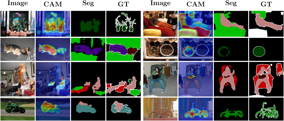
Figure 14: Illustrations of CoSA failure Cases. Different colors represent different categories: black: background; white: ignore areas; : plant; : person; : sofa; : dog; : cat; : chair; : motorbike; : bicycle. The activated classes in the demonstration from left to right and from top to bottom are: plant, sofa, dog, plant, person, cat, person, bicycle.

More visualizations of our CoSA results are given in Fig. 10 for VOC and Fig. 11, Fig. 12 for COCO. When compared to other SOTA models, CoSA exhibits i) better foreground-background separation (evidenced in R2–R3 in Fig. 10 and R1–R10 in Fig. 11); ii) more robust to inter-class variation and occlusion (affirmed in R4–R7 in Fig. 10 and R1–R4 in Fig. 12). iii) less coexistence problem (demonstrated in R9–R11 in Fig. 10 and R8– R10 in Fig. 12); Last but not least, our CoSA can reveal certain limitations in manual GT segmentation, as depicted in R8 in Fig. 10 and R5–R7 in Fig. 12. We also show our CoSA results on VOC test set in Fig. 14 and some failure cases in Fig. 14.

Appendix B Further Analysis

Impact of CRF. The conditional random field (CRF) proposes to optimize the segmentation by utilizing the low-level information obtained from the local interactions of pixels and edges [10]. Traditionally, a manually designed CRF postprocessing step has been widely adopted for refining segmentation [15, 50] or CAMs [51, 65, 70] in WSSS. As our aim is to develop a fully end-to-end WSSS solution, incorporating CRF postprocessing contradicts this principal. Through our experiments, we demonstrate that CoSA, unlike other single-stage methods, does not heavily depend on CRF. Our results indicate that incorporating CRF results in marginal improvement of $0.2\%$, $0.1\%$, and $0.1\%$ for VOC val, VOC test, and COCO val, respectively, as presented in Tab. 2 of the main paper. Tab. 6(a) suggests that in comparison to other SOTA models, our CoSA exhibits a lesser dependency on the CRF postprocessing. On the contrary, eliminating the CRF step leads to a noteworthy enhancement of 165% in terms of inference speed, as demonstrated in Tab. 6(b).

(a)
Method w/o CRF w/ CRF AFA [52] 63.8 66.0 (+2.2) VIT-PCM [51] 67.7 71.4 (+3.7) ToCo [53] 69.2 71.1 (+0.9) CoSA 76.2 76.4 (+0.2)

(b)
CoSA Speed w/o CRF 4.11 imgs/s w/ CRF 1.83 imgs/s

Table 6: CRF Impact. (a): Comparisons of CRF impact on SOTA single-stage WSSS methods on VOC val. (b): Inference speed with and without CRF. Speed tested using a single 3090 GPU.

	CAMs	CAMs	Seg.	Total	mIoU
	Generation	Refinement	Training
MCT [65]	2.2hrs (21M)	11.1hrs (106M)	15.5hrs (124M)	28.8hrs (251M)	71.6
BECO [50]	0.9hrs (23M)	6.5hrs  (24M)	22.2hrs  (91M)	29.6hrs (138M)	71.8
ToCo [53]	9.9hrs  (98M)			9.9hrs  (98M)	72.2
	CAMs and Seg. Co-optimization
CoSA	8.7hrs  (92M)			8.7hrs (92M)	75.1

Table 7: Training Speed and Parameters Comparisons. We report the detailed training time, parameters and final mIoU on VOC test split for MCT, BECO, ToCo and our CoSA. All methods are tested using the same machine with a single 3090 GPU. The official MCT, BECO and ToCo code repositories are utilized in this study.

Transformation	Description	Parameter Setting
RandomRescale	Rescale the image by $r$ times, $r$ randomly sampled from $r\sim U(r_{min},r_{max})$.	$r_{min}=0.5,r_{max}=2$
RandomFlip	Randomly horizontally flip a image with probability of $p$.	$p=0.5$
RandomCrop	Randomly crop a image by a hight $h$ and a width $w$.	$w=448,h=448$
GaussianBlur	Randomly blur a image with probability of $p$.	$p=0.5$

Table 8: Weak data augmentation $\mathcal{T}_{w}$ for the input of assignment network.

Transformation	Description	Parameter Setting
RandomRescale	Rescale the image by $r$ times, $r$ randomly sampled from $r\sim U(r_{min},r_{max})$.	$r_{min}=0.5,r_{max}=2$
RandomFlip	Randomly horizontally flip a image with probability of $p$.	$p=0.5$
RandomCrop	Randomly crop a image by a hight $h$ and a width $w$.	$w=448,h=448$
GaussianBlur	Randomly blur a image with probability of $p$.	$p=0.5$
OneOf	Select one of the transformation in a transformation set $T$.	$T=$ TransAppearance

Table 9: Strong data augmentation $\mathcal{T}_{s}$ for the input of online network image.

Transformation	Description	Parameter Setting
Identity	Returns the original image.
Autocontrast	Maximizes the image contrast by setting the darkest (lightest) pixel to black (white).
Equalize	Equalizes the image histogram.
RandSolarize	Invert all pixels above a threshold value $T$.	$T\in U(0,1)$
RandColor	Adjust the color balance. $C=0$ returns a black&white image, $C=1$ returns the original image.	$C\in U(0.05,0.95)$
RandContrast	Adjust the contrast. $C=0$ returns a solid grey image, $C=1$ returns the original image.	$C\in U(0.05,0.95)$
RandBrightness	Adjust the brightness. $C=0$ returns a black image, $C=1$ returns the original image.	$C\in U(0.05,0.95)$
RandSharpness	Adjust the sharpness. $C=0$ returns a blurred image, $C=1$ returns the original image.	$C\in U(0.05,0.95)$
RandPolarize	Reduce each pixel to $C$ bits.	$C\in U(4,8)$

Table 10: Appearance transformations, called TransAppearance, used in strong data augmentation.

Efficiency Study. Unlike multi-stage approaches, CoSA is extremely efficient in training. It can be trained end-to-end efficiently. When training a semantic segmentation model with weak labels on the VOC dataset, our method requires a mere 8.7 hours of training time and a total of 92M parameters. In contrast, MCT [65] would necessitate approximately 231% more time (20.1hrs $\uparrow$) and 173% more parameters (159M $\uparrow$) for the same task, and BECO [50] would require around 240% more time (20.9hrs $\uparrow$) and 50% more parameters (46M $\uparrow$). When compared to the single-stage method, CoSA also demonstrate its advantage in speed-accuracy trade-off. Further details regarding the efficiency study can be found in Tab. 7.

Algorithm 1 CoSA Training Pseudo Code

1:Require: $\mathcal{D}$ $\triangleright$ image-level classification dataset

2:Require: $\mathcal{F}_{\Theta},~{}\mathcal{F}_{\Theta^{\prime}}$ $\triangleright$ online network parameterized by $\Theta$ and assignment network by $\Theta^{\prime}$

3:$\mathcal{F}_{\Theta}$ $\leftarrow$ Init,   $\mathcal{F}_{\Theta^{\prime}}$ $\leftarrow$ Init $\triangleright$ initialize networks with pretrained backbone

4:do

5:     $x$, $Y_{\text{gt}}$ $\leftarrow$ Sample($\mathcal{D}$) $\triangleright$ sample a mini-batch of image and weak-label pairs

6:     $x_{s},x_{w}$ $\leftarrow$ $\mathcal{T}_{s}(x),\mathcal{T}_{w}(x)$ $\triangleright$ apply strong and weak augumentations

7:     $\{x_{w}^{s}\}$ $\leftarrow$ $\texttt{multiscale}(x_{w})$ $\triangleright$ generate a set of $x_{w}$ with different scales

8:     $\{\mathcal{M}^{\prime},~{}\mathcal{M}^{\dagger\prime},~{}\mathcal{S}^{\prime}\}$ $\leftarrow$ $\mathcal{F}_{\Theta^{\prime}}(\{x_{w}^{s}\})$ $\triangleright$ forward a set of $x_{w}$ in assignment network

9:     $\mathcal{M}^{\prime},~{}\mathcal{M}^{\dagger\prime},~{}\mathcal{S}^{\prime}$ $\leftarrow$ Maxpool$(\{\mathcal{M}^{\prime}\})$, Maxpool$(\{\mathcal{M}^{\dagger\prime}\})$, Avgpool$(\{\mathcal{S}^{\prime}\})$ $\triangleright$ ensemble multiscale outputs

10:     $\mathcal{M}^{\prime},~{}\mathcal{M}^{\dagger\prime},~{}\mathcal{S}^{\prime}$ $\leftarrow$ Filter$(\mathcal{M}^{\prime},~{}\mathcal{M}^{\dagger\prime},~{}\mathcal{S}^{\prime})$, $\triangleright$ filter CAMs and segmentation prediction with $Y_{\text{gt}}$

11:     $Z,~{}Z^{\dagger},~{}\mathcal{M},~{}\mathcal{M}^{\dagger},~{}\mathcal{S}$ $\leftarrow$ $\mathcal{F}_{\Theta}(x_{s})$ $\triangleright$ forward $x_{s}$ in online network

12:     $\mathcal{L}_{\text{cls}}+\mathcal{L}_{\text{cls}}^{\mathcal{M}^{\dagger}}$ $\leftarrow$ $\mathcal{L}_{\text{cls}}(Z,Y_{\text{gt}})+\mathcal{L}_{\text{cls}}(Z^{\dagger},Y_{\text{gt}})$ $\triangleright$ get classification losses for $\mathcal{M}$ and $\mathcal{M}^{\dagger}$ by eq. (1)

13:     $\xi^{\star}$ $\leftarrow$ solve eq. (6) with $\mathcal{M}^{\prime}$ $\triangleright$ get dynamic threshold

14:     $\hat{\mathcal{Y}}^{\text{CPL}}$ $\leftarrow$ eq. (2) with $\mathcal{M}^{\prime},~{}\xi^{\star}$ $\triangleright$ obtain CPL

15:     ${\mathcal{P}}$ $\leftarrow$ eq. (4) with $\mathcal{M}^{\prime},~{}\xi^{\star}$ $\triangleright$ estimate perplexity score

16:     ${\mathcal{L}_{\text{c2s}}}$ $\leftarrow$ eq. (5) with $\hat{\mathcal{Y}}^{\text{CPL}},\mathcal{S},~{}{\mathcal{P}}$ $\triangleright$ get CAM2seg loss

17:     ${\mathcal{L}_{\text{c2s}}^{\mathcal{M}^{\dagger}}}$ $\leftarrow$ follow 14 – 17 but with $\mathcal{M}^{\dagger\prime}$ $\triangleright$ get another CAM2seg loss

18:     $\hat{\mathcal{Y}}^{\text{SPL}}$ $\leftarrow$ eq. (7) with $\mathcal{S}^{\prime}$ $\triangleright$ obtain SPL

19:     ${\mathcal{L}_{\text{s2c}}}$ $\leftarrow$ eq. (8) with $\hat{\mathcal{Y}}^{\text{SPL}},~{}\mathcal{M}$ $\triangleright$ get Seg2CAM loss

20:     $\mathcal{R}^{+},~{}\mathcal{R}^{-}$ $\leftarrow$ eq. (9) with $\mathcal{P},~{}\hat{\mathcal{Y}}^{\text{CPL}}$ $\triangleright$ define positive and negative correlation matrix

21:     ${\mathcal{L}_{\text{csc}}}$ $\leftarrow$ eq. (10) with $\mathcal{M},~{}\mathcal{R}^{+},~{}\mathcal{R}^{-}$ $\triangleright$ get contrastive seperation loss

22:     $\mathcal{L}_{\text{CoSA}}$ $\leftarrow$ $\!\mathcal{L}_{\text{cls}}\!+\mathcal{L}_{\text{cls}}^{\mathcal{M}^{\dagger}}\!\!+\!\lambda_{\text{c2s}}\big{(}\mathcal{L}_{\text{c2s}}\!+\!\mathcal{L}_{\text{c2s}}^{\mathcal{M}^{\dagger}}\big{)}\!+\!\lambda_{\text{s2c}}\mathcal{L}_{\text{s2c}}+\!\lambda_{\text{csc}}\mathcal{L}_{\text{csc}}.$ $\triangleright$ weighted sum as the overall training objective

23:     $\Delta\Theta$ $\leftarrow$ $-\nabla_{\mathcal{L}_{\text{CoSA}}}\Theta$ $\triangleright$ backpropagate the overall loss

24:     $\Theta$ $\leftarrow$ $\Theta+\Delta\Theta$ $\triangleright$ undate online network with gradient

25:     $\Theta^{\prime}$ $\leftarrow$ $m\Theta^{\prime}+(1-m)\Theta$$\triangleright$ undate assignment network via EMA

26:until $\mathcal{L}_{\text{CoSA}}$ converge

27:end

Method	bkg	plane	bike	bird	boat	bottle	bus	car	cat	chair	cow
AdvCAM [34] CVPR21	90.0	79.8	34.1	82.6	63.3	70.5	89.4	76.0	87.3	31.4	81.3
MCT [65] CVPR22	91.9	78.3	39.5	89.9	55.9	76.7	81.8	79.0	90.7	32.6	87.1
ToCo [53] CVPR23	91.1	80.6	48.7	68.6	45.4	79.6	87.4	83.3	89.9	35.8	84.7
Xu et al. [66] CVPR23	92.4	84.7	42.2	85.5	64.1	77.4	86.6	82.2	88.7	32.7	83.8
BECO [50] CVPR23	91.1	81.8	33.6	87.0	63.2	76.1	92.3	87.9	90.9	39.0	90.2
CoSA* (Ours)	93.1	85.5	48.5	88.7	70.0	77.6	90.4	86.4	90.3	47.2	88.7
Method	table	dog	horse	mbike	person	plant	sheep	sofa	train	tv	mIoU
AdvCAM [34] CVPR21	33.1	82.5	80.8	74.0	72.9	50.3	82.3	42.2	74.1	52.9	68.1
MCT [65] CVPR22	57.2	87.0	84.6	77.4	79.2	55.1	89.2	47.2	70.4	58.8	71.9
ToCo [53] CVPR23	60.5	83.7	83.7	76.8	83.0	56.6	87.9	43.5	60.5	63.1	71.1
Xu et al. [66] CVPR23	59.0	82.4	80.9	76.1	81.4	48.0	88.2	46.4	70.2	62.5	72.2
BECO [50] CVPR23	41.6	85.9	86.3	81.8	76.7	56.7	89.5	54.7	64.3	60.6	72.9
CoSA* (Ours)	54.1	87.3	87.1	79.6	85.6	53.2	89.9	71.9	65.1	63.4	76.4

Table 11: Per-class Segmentation on VOC val Split. Comparison of per-class segmentation results on VOC val. CoSA is compared with AdvCAM, MCTformer, ToCo, Xu et al. and BECO. Best results are in bold.

Method	bkg	plane	bike	bird	boat	bottle	bus	car	cat	chair	cow
AdvCAM [34] CVPR21	90.1	81.2	33.6	80.4	52.4	66.6	87.1	80.5	87.2	28.9	80.1
MCT [65] CVPR22	90.9	76.0	37.2	79.1	54.1	69.0	78.1	78.0	86.1	30.3	79.5
ToCo [53] CVPR23	91.5	88.4	49.5	69.0	41.6	72.5	87.0	80.7	88.6	32.2	85.0
CoSA* (Ours)	93.3	88.1	47.0	84.2	60.2	75.0	87.7	81.7	92.0	34.5	87.8
Method	table	dog	horse	mbike	person	plant	sheep	sofa	train	tv	mIoU
AdvCAM [34] CVPR21	38.5	84.0	83.0	79.5	71.9	47.5	80.8	59.1	65.4	49.7	68.0
MCT [65] CVPR22	58.3	81.7	81.1	77.0	76.4	49.2	80.0	55.1	65.4	54.5	68.4
ToCo [53] CVPR23	68.4	81.4	85.6	83.2	83.4	68.2	88.9	55.0	49.3	65.0	72.2
CoSA* (Ours)	59.6	86.2	86.3	84.9	82.8	68.2	87.4	63.9	67.7	61.6	75.2

Table 12: Per-class Segmnetation on VOC test Split. Comparison of per-class segmentation results on VOC test. Results from AdvCAM, MCT, and ToCo are used for this comparison. Best results are in bold.

Class	MCT[65] (CVPR22)	Xu et al. [66] (CVPR23)	ToCo[53] (CVPR23)	CoSA (Ours)	Class	MCT[65] (CVPR22)	Xu et al. [66] (CVPR23)	ToCo[53] (CVPR23)	CoSA (Ours)
background	82.4	85.3	68.5	84.0	wine glass	27.0	33.8	20.6	42.1
person	62.6	72.9	28.1	70.3	cup	29.0	35.8	26.0	33.1
bicycle	47.4	49.8	39.7	52.4	fork	23.4	20.0	7.6	24.2
car	47.2	43.8	38.9	54.3	knife	12.0	12.6	18.4	32.9
motorcycle	63.7	66.2	55.1	71.9	spoon	6.6	6.7	3.0	9.0
airplane	64.7	69.2	62.1	74.0	bowl	22.4	23.7	19.8	22.8
bus	64.5	69.1	39.0	77.2	banana	63.2	64.4	71.5	69.3
train	64.5	63.7	48.7	60.0	apple	44.4	50.8	55.5	61.3
truck	44.8	43.4	37.3	55.4	sandwich	39.7	47.0	41.2	48.3
boat	42.3	42.3	49.1	52.1	orange	63.0	64.6	70.6	69.2
traffic light	49.9	49.3	47.3	55.1	broccoli	51.2	50.6	56.7	52.8
fire hydrant	73.2	74.9	69.6	78.8	carrot	40.0	38.6	46.4	59.4
stop sign	76.6	77.3	70.1	82.2	hot dog	53.0	54.0	60.1	59.9
parking meter	64.4	67.0	67.9	71.5	pizza	62.2	64.1	54.9	56.5
bench	32.8	34.1	43.9	50.2	donut	55.7	59.7	61.1	71.1
bird	62.6	63.1	58.6	65.4	cake	47.9	50.6	42.5	57.0
cat	78.2	76.2	74.0	79.8	chair	22.8	24.5	24.1	33.8
dog	68.2	70.6	64.0	72.8	couch	35.0	40.0	44.2	58.1
horse	65.8	67.1	66.1	71.4	potted plant	13.5	13.0	27.4	23.5
sheep	70.1	70.8	67.9	74.3	bed	48.6	53.7	54.0	61.5
cow	68.3	71.2	69.0	74.0	dining table	12.9	19.2	25.6	29.2
elephant	81.6	82.2	79.7	81.9	toilet	63.1	66.6	62.0	69.7
bear	80.1	79.6	76.8	85.3	tv	47.9	50.8	49.1	53.2
zebra	83.0	82.8	77.5	76.3	laptop	49.5	55.4	55.7	63.9
giraffe	76.9	76.7	66.1	68.5	mouse	13.4	14.4	8.6	16.4
backpack	14.6	17.5	20.3	28.6	remote	41.9	47.1	56.6	49.1
umbrella	61.7	66.9	70.9	73.4	keyboard	49.8	57.2	41.8	49.6
handbag	4.5	5.8	8.1	11.9	cellphone	54.1	54.9	58.5	66.2
tie	25.2	31.4	33.4	47.7	microwave	38.0	46.1	55.5	53.2
suitcase	46.8	51.4	55.3	63.8	oven	29.9	35.3	36.2	49.2
frisbee	43.8	54.1	39.6	63.1	toaster	0.0	2.0	0.0	0.0
skis	12.8	13.0	4.0	22.5	sink	28.0	36.1	19.0	41.9
snowboard	31.4	30.3	15.5	40.5	refrigerator	40.1	52.7	51.9	62.0
sports ball	9.2	36.1	11.0	33.1	book	32.2	34.8	31.5	37.8
kite	26.3	47.5	40.7	59.9	clock	43.2	51.5	32.9	55.2
baseball bat	0.9	7.0	1.8	3.8	vase	22.6	25.8	33.3	33.8
baseball glove	0.7	10.4	17.6	37.9	scissors	32.9	30.7	49.8	54.7
skateboard	7.8	15.2	13.3	12.5	teddy bear	61.9	61.4	67.5	69.3
surfboard	46.5	51.5	21.5	16.5	hair drier	0.0	1.3	10.0	0.3
tennis racket	1.4	26.4	6.8	7.2	toothbrush	12.2	19.0	29.3	39.3
bottle	31.1	37.1	25.7	35.1	mIoU	42.0	45.9	42.4	51.1

Table 13: Per-class Segmentation on COCO val Split. Comparison of per-class segmentation results on the COCO 2014 val set. CoSA is compared with MCTformer, Xu et al. and ToCo. Best results are in bold.

Appendix C Further Implementation Details

CoSA Implementation Details. For image preprocessing, weak transformation $\mathcal{T}_{w}$ and strong transformation $\mathcal{T}_{s}$ are employed in CoSA for the input of assignment network and online network, respectively. $\mathcal{T}_{w}$ and $\mathcal{T}_{s}$ details are given in Tab. 10 and Tab. 10. Following [53], we use the multi-scale inference in assignment network to produce CPL and SPL. For VOC training, CoSA is warmed up with 6K iterations, where $\lambda_{\text{c2s}}$, $\lambda_{\text{c2s}}$, and $\lambda_{\text{csc}}$ are set to $0$. In practice, we train CoSA for 20K iterations on 2 GPUs, with 2 images per GPU, or for 40K iterations on 1 GPU for some ablation experiments. For COCO training, CoSA is warmed up with 10K iterations and is trained on 2 GPUs, handling 4 images per GPU across 40K iterations.

CoSA-MS Implementation Details. Tab. 2 in the main paper presents the segmentation results of the multi-stage version of our approach, known as CoSA-MS. In those experiments, we leverage the CAM pseudo-labels generated by our CoSA to directly train standalone segmentation networks. It is important to note that we do not use PSA [2], which is widely used in [65, 15], nor IRN [1], extensively used in [50, 12, 59, 31], for CPL post-refinement. For our R101 segmentation network, we use a ResNet101 version of DeepLabV3+ model, same as BECO [50]. As for the CoSA-MS with WR38 network, we utilize a encoder-decoder framework, where encoder is WideResNet38 [61] and decoder is LargeFoV [10], following the final step described in MCT [65]. Regarding the SWIN implementation, we use the SWIN-Base encoder [44] in conjunction with UperNet decoder [62], following the description in [14, 12].

Training Pseudo Code. we present the pseudo code for training CoSA in Algorithm 1.

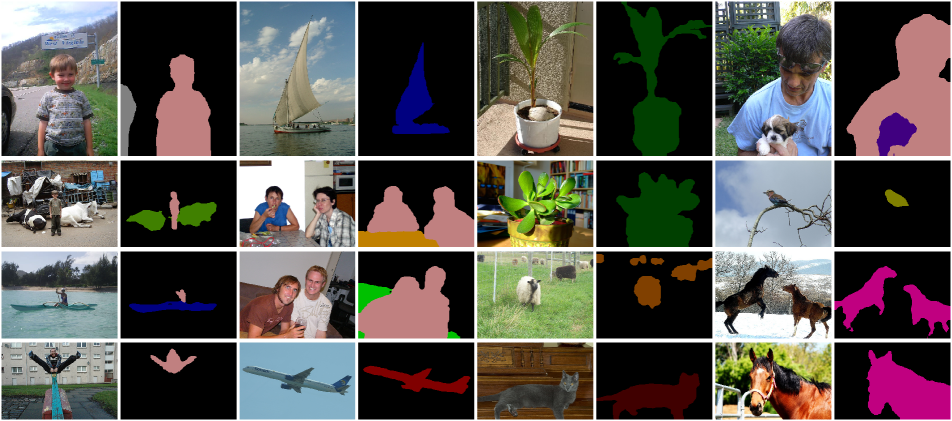
Figure 13: Visualization on VOC test. Different colors represent different categories: black: background; : car; : person; : boat; : plant; : dog; : cow. : dining-table. : bird; : sofa; : sheep; : house; : airplane; : cat.

References

- [1] Jiwoon Ahn, Sunghyun Cho, and Suha Kwak. Weakly supervised learning of instance segmentation with inter-pixel relations. In IEEE Computer Vision and Pattern Recognition (CVPR), pages 2209–2218, 2019.
- [2] Jiwoon Ahn and Suha Kwak. Learning pixel-level semantic affinity with image-level supervision for weakly supervised semantic segmentation. In IEEE Computer Vision and Pattern Recognition (CVPR), pages 4981–4990, 2018.
- [3] Nikita Araslanov and Stefan Roth. Single-stage semantic segmentation from image labels. In IEEE Computer Vision and Pattern Recognition (CVPR), pages 4253–4262, 2020.
- [4] Amy Bearman, Olga Russakovsky, Vittorio Ferrari, and Li Fei-Fei. What’s the point: Semantic segmentation with point supervision. In European Conference on Computer Vision (ECCV), pages 549–565. Springer, 2016.
- [5] Mathilde Caron, Ishan Misra, Julien Mairal, Priya Goyal, Piotr Bojanowski, and Armand Joulin. Unsupervised learning of visual features by contrasting cluster assignments. Neural Information Processing Systems (NeurIPS), 33:9912–9924, 2020.
- [6] Mathilde Caron, Hugo Touvron, Ishan Misra, Hervé Jégou, Julien Mairal, Piotr Bojanowski, and Armand Joulin. Emerging properties in self-supervised vision transformers. In IEEE Computer Vision and Pattern Recognition (CVPR), pages 9650–9660, 2021.
- [7] Aditya Chattopadhay, Anirban Sarkar, Prantik Howlader, and Vineeth N Balasubramanian. Grad-cam++: Generalized gradient-based visual explanations for deep convolutional networks. In IEEE Winter Conference on Applications of Computer Vision (WACV), pages 839–847. IEEE, 2018.
- [8] Liyi Chen, Chenyang Lei, Ruihuang Li, Shuai Li, Zhaoxiang Zhang, and Lei Zhang. Fpr: False positive rectification for weakly supervised semantic segmentation. In IEEE International Conference on Computer Vision (ICCV), pages 1108–1118, 2023.
- [9] Liyi Chen, Weiwei Wu, Chenchen Fu, Xiao Han, and Yuntao Zhang. Weakly supervised semantic segmentation with boundary exploration. In European Conference on Computer Vision (ECCV), pages 347–362. Springer, 2020.
- [10] Liang-Chieh Chen, George Papandreou, Iasonas Kokkinos, Kevin Murphy, and Alan L Yuille. Deeplab: Semantic image segmentation with deep convolutional nets, atrous convolution, and fully connected crfs. IEEE Transactions on Pattern Analysis and Machine Intelligence (TPAMI), 40(4):834–848, 2017.
- [11] Qi Chen, Lingxiao Yang, Jian-Huang Lai, and Xiaohua Xie. Self-supervised image-specific prototype exploration for weakly supervised semantic segmentation. In IEEE Computer Vision and Pattern Recognition (CVPR), pages 4288–4298, 2022.
- [12] Zhaozheng Chen and Qianru Sun. Extracting class activation maps from non-discriminative features as well. In IEEE Computer Vision and Pattern Recognition (CVPR), pages 3135–3144, 2023.
- [13] Zhang Chen, Zhiqiang Tian, Jihua Zhu, Ce Li, and Shaoyi Du. C-cam: Causal cam for weakly supervised semantic segmentation on medical image. In IEEE Computer Vision and Pattern Recognition (CVPR), pages 11676–11685, 2022.
- [14] Zhaozheng Chen, Tan Wang, Xiongwei Wu, Xian-Sheng Hua, Hanwang Zhang, and Qianru Sun. Class re-activation maps for weakly-supervised semantic segmentation. In IEEE Computer Vision and Pattern Recognition (CVPR), pages 969–978, 2022.
- [15] Zesen Cheng, Pengchong Qiao, Kehan Li, Siheng Li, Pengxu Wei, Xiangyang Ji, Li Yuan, Chang Liu, and Jie Chen. Out-of-candidate rectification for weakly supervised semantic segmentation. In IEEE Computer Vision and Pattern Recognition (CVPR), pages 23673–23684, 2023.
- [16] Jifeng Dai, Kaiming He, and Jian Sun. Boxsup: Exploiting bounding boxes to supervise convolutional networks for semantic segmentation. In IEEE International Conference on Computer Vision (ICCV), pages 1635–1643, 2015.
- [17] Alexey Dosovitskiy, Lucas Beyer, Alexander Kolesnikov, Dirk Weissenborn, Xiaohua Zhai, Thomas Unterthiner, Mostafa Dehghani, Matthias Minderer, Georg Heigold, Sylvain Gelly, et al. An image is worth 16x16 words: Transformers for image recognition at scale. In International Conference on Learning Representations (ICLR), 2021.
- [18] Ye Du, Zehua Fu, Qingjie Liu, and Yunhong Wang. Weakly supervised semantic segmentation by pixel-to-prototype contrast. In IEEE Computer Vision and Pattern Recognition (CVPR), pages 4320–4329, 2022.
- [19] Mark Everingham, Luc Van Gool, Christopher KI Williams, John Winn, and Andrew Zisserman. The pascal visual object classes (voc) challenge. International journal of computer vision (IJCV), 88:303–338, 2010.
- [20] Junsong Fan, Zhaoxiang Zhang, Tieniu Tan, Chunfeng Song, and Jun Xiao. Cian: Cross-image affinity net for weakly supervised semantic segmentation. In AAAI Conference on Artificial Intelligence (AAAI), volume 34, pages 10762–10769, 2020.
- [21] Wei Gao, Fang Wan, Xingjia Pan, Zhiliang Peng, Qi Tian, Zhenjun Han, Bolei Zhou, and Qixiang Ye. Ts-cam: Token semantic coupled attention map for weakly supervised object localization. In IEEE International Conference on Computer Vision (ICCV), pages 2886–2895, 2021.
- [22] Jean-Bastien Grill, Florian Strub, Florent Altché, Corentin Tallec, Pierre Richemond, Elena Buchatskaya, Carl Doersch, Bernardo Avila Pires, Zhaohan Guo, Mohammad Gheshlaghi Azar, et al. Bootstrap your own latent-a new approach to self-supervised learning. Neural Information Processing Systems (NeurIPS), 33:21271–21284, 2020.
- [23] Bharath Hariharan, Pablo Arbeláez, Lubomir Bourdev, Subhransu Maji, and Jitendra Malik. Semantic contours from inverse detectors. In IEEE International Conference on Computer Vision (ICCV), pages 991–998. IEEE, 2011.
- [24] Bharath Hariharan, Pablo Arbeláez, Ross Girshick, and Jitendra Malik. Hypercolumns for object segmentation and fine-grained localization. In IEEE Computer Vision and Pattern Recognition (CVPR), pages 447–456, 2015.
- [25] Geoffrey Hinton, Oriol Vinyals, and Jeff Dean. Distilling the knowledge in a neural network. arXiv preprint arXiv:1503.02531, 2015.
- [26] Peng-Tao Jiang, Yuqi Yang, Qibin Hou, and Yunchao Wei. L2g: A simple local-to-global knowledge transfer framework for weakly supervised semantic segmentation. In IEEE Computer Vision and Pattern Recognition (CVPR), pages 16886–16896, 2022.
- [27] Tsung-Wei Ke, Jyh-Jing Hwang, and Stella Yu. Universal weakly supervised segmentation by pixel-to-segment contrastive learning. In International Conference on Learning Representations (ICLR), 2020.
- [28] Anna Khoreva, Rodrigo Benenson, Jan Hosang, Matthias Hein, and Bernt Schiele. Simple does it: Weakly supervised instance and semantic segmentation. In IEEE Computer Vision and Pattern Recognition (CVPR), pages 876–885, 2017.
- [29] Philipp Krähenbühl and Vladlen Koltun. Efficient inference in fully connected crfs with gaussian edge potentials. Neural Information Processing Systems (NeurIPS), 24, 2011.
- [30] Hyeokjun Kweon, Sung-Hoon Yoon, Hyeonseong Kim, Daehee Park, and Kuk-Jin Yoon. Unlocking the potential of ordinary classifier: Class-specific adversarial erasing framework for weakly supervised semantic segmentation. In IEEE International Conference on Computer Vision (ICCV), pages 6994–7003, 2021.
- [31] Hyeokjun Kweon, Sung-Hoon Yoon, and Kuk-Jin Yoon. Weakly supervised semantic segmentation via adversarial learning of classifier and reconstructor. In IEEE Computer Vision and Pattern Recognition (CVPR), pages 11329–11339, 2023.
- [32] Jungbeom Lee, Eunji Kim, Sungmin Lee, Jangho Lee, and Sungroh Yoon. Ficklenet: Weakly and semi-supervised semantic image segmentation using stochastic inference. In IEEE Computer Vision and Pattern Recognition (CVPR), pages 5267–5276, 2019.
- [33] Jungbeom Lee, Eunji Kim, Jisoo Mok, and Sungroh Yoon. Anti-adversarially manipulated attributions for weakly supervised semantic segmentation and object localization. IEEE Transactions on Pattern Analysis and Machine Intelligence (TPAMI), 2022.
- [34] Jungbeom Lee, Eunji Kim, and Sungroh Yoon. Anti-adversarially manipulated attributions for weakly and semi-supervised semantic segmentation. In IEEE Computer Vision and Pattern Recognition (CVPR), pages 4071–4080, 2021.
- [35] Jungbeom Lee, Seong Joon Oh, Sangdoo Yun, Junsuk Choe, Eunji Kim, and Sungroh Yoon. Weakly supervised semantic segmentation using out-of-distribution data. In IEEE Computer Vision and Pattern Recognition (CVPR), pages 16897–16906, 2022.
- [36] Jungbeom Lee, Jihun Yi, Chaehun Shin, and Sungroh Yoon. Bbam: Bounding box attribution map for weakly supervised semantic and instance segmentation. In IEEE Computer Vision and Pattern Recognition (CVPR), pages 2643–2652, 2021.
- [37] Seungho Lee, Minhyun Lee, Jongwuk Lee, and Hyunjung Shim. Railroad is not a train: Saliency as pseudo-pixel supervision for weakly supervised semantic segmentation. In IEEE Computer Vision and Pattern Recognition (CVPR), pages 5495–5505, 2021.
- [38] Jing Li, Junsong Fan, and Zhaoxiang Zhang. Towards noiseless object contours for weakly supervised semantic segmentation. In IEEE Computer Vision and Pattern Recognition (CVPR), pages 16856–16865, 2022.
- [39] Jinlong Li, Zequn Jie, Xu Wang, Lin Ma, et al. Expansion and shrinkage of localization for weakly-supervised semantic segmentation. In Neural Information Processing Systems (NeurIPS), 2022.
- [40] Yi Li, Yiqun Duan, Zhanghui Kuang, Yimin Chen, Wayne Zhang, and Xiaomeng Li. Uncertainty estimation via response scaling for pseudo-mask noise mitigation in weakly-supervised semantic segmentation. In AAAI Conference on Artificial Intelligence (AAAI), volume 36, pages 1447–1455, 2022.
- [41] Tsung-Yi Lin, Michael Maire, Serge Belongie, James Hays, Pietro Perona, Deva Ramanan, Piotr Dollár, and C Lawrence Zitnick. Microsoft coco: Common objects in context. In European Conference on Computer Vision (ECCV), pages 740–755. Springer, 2014.
- [42] Yuqi Lin, Minghao Chen, Wenxiao Wang, Boxi Wu, Ke Li, Binbin Lin, Haifeng Liu, and Xiaofei He. Clip is also an efficient segmenter: A text-driven approach for weakly supervised semantic segmentation. In IEEE Computer Vision and Pattern Recognition (CVPR), pages 15305–15314, 2023.
- [43] Sheng Liu, Kangning Liu, Weicheng Zhu, Yiqiu Shen, and Carlos Fernandez-Granda. Adaptive early-learning correction for segmentation from noisy annotations. In IEEE Computer Vision and Pattern Recognition (CVPR), pages 2606–2616, 2022.
- [44] Ze Liu, Yutong Lin, Yue Cao, Han Hu, Yixuan Wei, Zheng Zhang, Stephen Lin, and Baining Guo. Swin transformer: Hierarchical vision transformer using shifted windows. In IEEE International Conference on Computer Vision (ICCV), pages 10012–10022, 2021.
- [45] Zhengzhe Liu, Xiaojuan Qi, and Chi-Wing Fu. One thing one click: A self-training approach for weakly supervised 3d semantic segmentation. In IEEE Computer Vision and Pattern Recognition (CVPR), pages 1726–1736, 2021.
- [46] Ilya Loshchilov and Frank Hutter. Decoupled weight decay regularization. arXiv preprint arXiv:1711.05101, 2017.
- [47] Aaron van den Oord, Yazhe Li, and Oriol Vinyals. Representation learning with contrastive predictive coding. arXiv preprint arXiv:1807.03748, 2018.
- [48] Maxime Oquab, Timothée Darcet, Théo Moutakanni, Huy Vo, Marc Szafraniec, Vasil Khalidov, Pierre Fernandez, Daniel Haziza, Francisco Massa, Alaaeldin El-Nouby, et al. Dinov2: Learning robust visual features without supervision. arXiv preprint arXiv:2304.07193, 2023.
- [49] Boris T Polyak and Anatoli B Juditsky. Acceleration of stochastic approximation by averaging. SIAM journal on control and optimization, 30(4):838–855, 1992.
- [50] Shenghai Rong, Bohai Tu, Zilei Wang, and Junjie Li. Boundary-enhanced co-training for weakly supervised semantic segmentation. In IEEE Computer Vision and Pattern Recognition (CVPR), pages 19574–19584, 2023.
- [51] Simone Rossetti, Damiano Zappia, Marta Sanzari, Marco Schaerf, and Fiora Pirri. Max pooling with vision transformers reconciles class and shape in weakly supervised semantic segmentation. In European Conference on Computer Vision (ECCV), pages 446–463. Springer, 2022.
- [52] Lixiang Ru, Yibing Zhan, Baosheng Yu, and Bo Du. Learning affinity from attention: end-to-end weakly-supervised semantic segmentation with transformers. In IEEE Computer Vision and Pattern Recognition (CVPR), pages 16846–16855, 2022.
- [53] Lixiang Ru, Heliang Zheng, Yibing Zhan, and Bo Du. Token contrast for weakly-supervised semantic segmentation. In IEEE Computer Vision and Pattern Recognition (CVPR), pages 3093–3102, 2023.
- [54] David Ruppert. Efficient estimations from a slowly convergent robbins-monro process. Technical report, Cornell University Operations Research and Industrial Engineering, 1988.
- [55] Ramprasaath R Selvaraju, Michael Cogswell, Abhishek Das, Ramakrishna Vedantam, Devi Parikh, and Dhruv Batra. Grad-cam: Visual explanations from deep networks via gradient-based localization. In IEEE International Conference on Computer Vision (ICCV), pages 618–626, 2017.
- [56] Wataru Shimoda and Keiji Yanai. Self-supervised difference detection for weakly-supervised semantic segmentation. In IEEE International Conference on Computer Vision (ICCV), pages 5208–5217, 2019.
- [57] Chunfeng Song, Yan Huang, Wanli Ouyang, and Liang Wang. Box-driven class-wise region masking and filling rate guided loss for weakly supervised semantic segmentation. In IEEE Computer Vision and Pattern Recognition (CVPR), pages 3136–3145, 2019.
- [58] Kunyang Sun, Haoqing Shi, Zhengming Zhang, and Yongming Huang. Ecs-net: Improving weakly supervised semantic segmentation by using connections between class activation maps. In IEEE Computer Vision and Pattern Recognition (CVPR), pages 7283–7292, 2021.
- [59] Changwei Wang, Rongtao Xu, Shibiao Xu, Weiliang Meng, and Xiaopeng Zhang. Treating pseudo-labels generation as image matting for weakly supervised semantic segmentation. In IEEE International Conference on Computer Vision (ICCV), pages 755–765, 2023.
- [60] Yude Wang, Jie Zhang, Meina Kan, Shiguang Shan, and Xilin Chen. Self-supervised equivariant attention mechanism for weakly supervised semantic segmentation. In IEEE Computer Vision and Pattern Recognition (CVPR), pages 12275–12284, 2020.
- [61] Zifeng Wu, Chunhua Shen, and Anton Van Den Hengel. Wider or deeper: Revisiting the resnet model for visual recognition. Pattern Recognition, 90:119–133, 2019.
- [62] Tete Xiao, Yingcheng Liu, Bolei Zhou, Yuning Jiang, and Jian Sun. Unified perceptual parsing for scene understanding. In European Conference on Computer Vision (ECCV), pages 418–434, 2018.
- [63] Jinheng Xie, Xianxu Hou, Kai Ye, and Linlin Shen. Clims: Cross language image matching for weakly supervised semantic segmentation. In IEEE Computer Vision and Pattern Recognition (CVPR), pages 4483–4492, 2022.
- [64] Jinheng Xie, Jianfeng Xiang, Junliang Chen, Xianxu Hou, Xiaodong Zhao, and Linlin Shen. C2am: Contrastive learning of class-agnostic activation map for weakly supervised object localization and semantic segmentation. In IEEE Computer Vision and Pattern Recognition (CVPR), pages 989–998, 2022.
- [65] Lian Xu, Wanli Ouyang, Mohammed Bennamoun, Farid Boussaid, and Dan Xu. Multi-class token transformer for weakly supervised semantic segmentation. In IEEE Computer Vision and Pattern Recognition (CVPR), pages 4310–4319, 2022.
- [66] Lian Xu, Wanli Ouyang, Mohammed Bennamoun, Farid Boussaid, and Dan Xu. Learning multi-modal class-specific tokens for weakly supervised dense object localization. In IEEE Computer Vision and Pattern Recognition (CVPR), pages 19596–19605, 2023.
- [67] Rongtao Xu, Changwei Wang, Jiaxi Sun, Shibiao Xu, Weiliang Meng, and Xiaopeng Zhang. Self correspondence distillation for end-to-end weakly-supervised semantic segmentation. In AAAI Conference on Artificial Intelligence (AAAI). AAAI Press, 2023.
- [68] Sung-Hoon Yoon, Hyeokjun Kweon, Jegyeong Cho, Shinjeong Kim, and Kuk-Jin Yoon. Adversarial erasing framework via triplet with gated pyramid pooling layer for weakly supervised semantic segmentation. In European Conference on Computer Vision (ECCV), pages 326–344. Springer, 2022.
- [69] Lu Yu, Wei Xiang, Juan Fang, Yi-Ping Phoebe Chen, and Lianhua Chi. ex-vit: A novel explainable vision transformer for weakly supervised semantic segmentation. Pattern Recognition, page 109666, 2023.
- [70] Bingfeng Zhang, Jimin Xiao, Yunchao Wei, Mingjie Sun, and Kaizhu Huang. Reliability does matter: An end-to-end weakly supervised semantic segmentation approach. In AAAI Conference on Artificial Intelligence (AAAI), volume 34, pages 12765–12772, 2020.
- [71] Xiaolin Zhang, Yunchao Wei, Jiashi Feng, Yi Yang, and Thomas S Huang. Adversarial complementary learning for weakly supervised object localization. In IEEE Computer Vision and Pattern Recognition (CVPR), pages 1325–1334, 2018.
- [72] Bolei Zhou, Aditya Khosla, Agata Lapedriza, Aude Oliva, and Antonio Torralba. Learning deep features for discriminative localization. In IEEE Computer Vision and Pattern Recognition (CVPR), pages 2921–2929, 2016.
- [73] Tianfei Zhou, Meijie Zhang, Fang Zhao, and Jianwu Li. Regional semantic contrast and aggregation for weakly supervised semantic segmentation. In IEEE Computer Vision and Pattern Recognition (CVPR), pages 4299–4309, 2022.