Zeroth-Order Sampling Methods for Non-Log-Concave Distributions: Alleviating Metastability by Denoising Diffusion

Abstract

This paper considers the problem of sampling from non-logconcave distribution, based on queries of its unnormalized density. It first describes a framework, Diffusion Monte Carlo (DMC), based on the simulation of a denoising diffusion process with its score function approximated by a generic Monte Carlo estimator. DMC is an oracle-based meta-algorithm, where its oracle is the assumed access to samples that generate a Monte Carlo score estimator. Then we provide an implementation of this oracle, based on rejection sampling, and this turns DMC into a true algorithm, termed Zeroth-Order Diffusion Monte Carlo (ZOD-MC). We provide convergence analyses by first constructing a general framework, i.e. a performance guarantee for DMC, without assuming the target distribution to be log-concave or satisfying any isoperimetric inequality. Then we prove that ZOD-MC admits an inverse polynomial dependence on the desired sampling accuracy, albeit still suffering from the curse of dimensionality. Consequently, for low dimensional distributions, ZOD-MC is a very efficient sampler, with performance exceeding latest samplers, including also-denoising-diffusion-based RDMC and RS-DMC. Last, we experimentally demonstrate the insensitivity of ZOD-MC to increasingly higher barriers between modes or discontinuity in non-convex potential.

Code at https://github.com/KevinRojas1499/ZOD-MC

1 Introduction

The problem of drawing samples from a distribution based on unnormalized density $\propto\exp(-V)$ (described by the potential $V$) is a fundamental statistical and algorithmic problem. This classical problem nevertheless remains as a research frontier, providing pivotal tools to applications such as decision making, statistical inference / estimation, uncertainty quantification, data assimilation, and molecular dynamics. Worth mentioning is that machine learning could benefit vastly from progress in sampling as well, not only because of its connection to inference, optimization and approximation, but also through modern domains such as diffusion generative modeling & differential privacy.

Recent years have seen rapid developments of sampling algorithms with quantitative and non-asymptotic theoretical guarantees. Many of the results are either based on discretizations of diffusion processes [11, 12, 33, 14, 24, 23] or gradient flows [27, 9, 16]. In order to develop such guarantees, it is necessary to make assumptions about the target distributions, for instance, that it satisfies an isoperimetric property, where standard requirements are log-concavity or functional inequalities [11, 36, 15, 7, 31]. However, there is empirical evidence that the corresponding algorithms struggle to sample from targets that have high barriers between modes that create metastability. Overcoming such issues is highly nontrivial and researchers have continued to develop new methods to tackle these problems.

Diffusion models have lately shown remarkable ability in the generative modeling setting, with applications including image, video, audio, and macromolecule generations. This created a wave of theoretical work that showed the ability of diffusion models to sample from distributions under minimal assumptions [13, 37, 4, 22, 20, 3, 10, 2]. However, these works all started with the assumption that there is access to an approximation of the score function with some accuracy. This is a reasonable assumption for the task of generative modeling when one spends enough efforts on the training of the score, but the task of sampling is different. A natural question is: can we leverage the insensitivity of diffusion models to multimodality to efficiently sample from unnormalized, non-log-concave density? This would require approximating the score, which is then used as an inner loop inside an outer loop that integrates reverse diffusion process to transport, e.g., Gaussian initial condition, to nearly the target distribution.

The seminal works by [18, 19] try to answer this question using Monte Carlo estimators of the score function and to provide theoretical guarantees. We also mention earlier work by [38, 29], whose theoretical guarantees are less clear but are based other interesting ideas. [18] proposed Reverse Diffusion Monte Carlo (RDMC), which estimates the score via LMC algorithm and relaxes the isoperimetric assumptions in the analysis of traditional sampling algorithms. However, their method relies on the usage of a small time window where isoperimetric properties hold. This leaves the problem of finding a good initialization for the diffusion process. To alleviate this issue, [19] developed an acceleration of RDMC, the Recursive Score Diffusion-based Monte Carlo (RS-DMC), which improves the non-asymptotic complexity to be quasi-polynomial in both dimension and inverse accuracy and gets rid of any isoperimetric assumption. Such work provides strong theoretical guarantees, however it requires a lot of computational power to get a high accuracy sampler. Additionally, both RDMC and RS-DMC are based on first-order queries (i.e. gradients of $V$), which brings extra computational and memory costs, in addition to requiring a continuous differentiable $V$. Motivated by these two observations, we create a sampler that only makes use of zeroth-order queries without assuming any isoperimetric conditions on the target distribution. Our contributions can be summarized as follows.

• We introduce an oracle-based meta-algorithm DMC (Diffusion Monte Carlo) and provide a non-asymptotic guarantee in KL-divergence in Theorem 1. Our result provides theoretical insight on the choice of optimal step-size in DMC as well as in denoising diffusion models (Sec. 3.2).

• We develop a novel algorithm ZOD-MC (Zeroth Order Diffusion-Monte Carlo) that uses zeroth-order queries and the global minimal value of the potential function to generate samples approximating the target distribution. In Corollary 1, we establish a zeroth-order query complexity upper bound for general target distributions satisfying mild smoothness and moment conditions. Our result is summarized and compared to other sampling algorithms in Table 1.

• The advantages of our algorithm are experimentally verified for non-log-concave target distributions. We demonstrate the insensitivity of our algorithm to various high barriers between modes, and the ability of correctly account for discontinuities in the potential.

Algorithms	Queries	Assumptions	Criterion	Oracle Complexity
LMC	first-order	LSI	KL	$\mathcal{O}(d\varepsilon^{-1})$
RDMC	first order	None	TV	$\exp(\mathcal{O}(\log(d))\tilde{\mathcal{O}}(\varepsilon^{-1}))$
RS-DMC	first-order	None	KL	$\exp(\mathcal{O}(\log^{3}(d\varepsilon^{-1})))$
Proximal Sampler	zeroth-order	log-concave	KL	$\mathcal{O}(d\varepsilon^{-1})$
ZOD-MC	zeroth-order	None	$\text{KL}+W_{2}$	$\exp(\tilde{\mathcal{O}}(d)\mathcal{O}(\log(\varepsilon^{-1})))$

Table 1: Comparison of ZOD-MC to LMC, RDMC, RS-DMC and the Proximal Sampler: Summary of isoperimetric assumptions and oracle complexities to generate a $\varepsilon$-accurate sample under different criterion. $\tilde{O}$ hides polylog$(d\varepsilon^{-1})$ factors. The zeroth-order oracle complexity of ZOD-MC is from Corollary 1 for achieving both $\varepsilon$ KL and $\varepsilon$ $W_{2}$ errors. These theoretical results suggest that in the absense of isoperimetric assumptions, ZOD-MC excels in low-dimensions.

2 Preliminaries

2.1 Diffusion Model

Diffusion model generates samples that are similar to training data, based on requiring the generated data to follow the same latent distribution $p$ as the training data. To do so, it considers a forward noising process that transforms a random variable into Gaussian noise. One most commonly used forward process is (a time reparameterization of) the Ornstein-Uhlenbeck (OU) process, given by the SDE:

$$\mathrm{d}X_{t}=-X_{t}\mathrm{d}t+\sqrt{2}\mathrm{d}B_{t},\quad X_{0}\sim p,$$ (1)

where $\{B_{t}\}_{t\geq 0}$ is the standard Brownian motion in $\mathbb{R}^{d}$. The OU process that solves (1) is in distribution equivalent to a sum of two independent random vectors: $X_{t}=e^{-t}X_{0}+\sqrt{1-e^{-2t}}Z,\quad\forall\ t\geq 0,$ where $(X_{0},Z)\sim p\otimes\gamma^{d}$ and $\gamma^{d}$ is the standard Gaussian distribution in $\mathbb{R}^{d}$. Denote $p_{t}=\text{Law}(X_{t})$ for all $t\geq 0$; if we consider a large, fixed terminal time $T$ of $\eqref{eq:FD OU}$, then $p_{T}$ is close to $\gamma^{d}$. Then, the denoising or backwards diffusion process, $\{\bar{X}_{t}\}_{0\leq 0\leq T}$, can be constructed by reversing the OU process from time $T$, meaning that $\text{Law}(\bar{X_{t}})\coloneqq\text{Law}(X_{T-t})$ for all $t\in[0,T]$. By doing so we obtain the denoising diffusion process which solves the following SDE:

$$\mathrm{d}\bar{X}_{t}=(\bar{X}_{t}+2\nabla\log p_{T-t}(\bar{X}_{t}))\mathrm{d}t+\sqrt{2}\mathrm{d}\bar{B}_{t},\quad\bar{X}_{0}\sim p_{T},\ 0\leq t\leq T,$$ (2)

where $\{\bar{B}_{t}\}_{0\leq t\leq T}$ is a Brownian motion in $\mathbb{R}^{d}$, independent of $\{B_{t}\}_{0\leq t\leq T}$ and $\nabla\ln p_{t}$ is usually referred as the score function for $p_{t}$. Although the denoising process initializes at $p_{T}$, we can’t generate exact samples from $p_{T}$. In practice, people consider the standard Gaussian initialization $\gamma^{d}$ due to the fact that $p_{T}$ is close to $\gamma^{d}$ when $T$ is large. The denosing process with the standard Gaussian initialization is given by

$$\mathrm{d}\tilde{X}_{t}=(\tilde{X}_{t}+2\nabla\log p_{T-t}(\tilde{X}_{t}))\mathrm{d}t+\sqrt{2}\mathrm{d}\bar{B}_{t},\quad\tilde{X}_{0}\sim\gamma^{d},\ 0\leq t\leq T.$$ (3)

By simulating this denoising process (3), we can achieve the goal of generating new samples. However, the denoising process (3) can’t be simulated directly due to the fact that the score function is not explicitly known. A widely applied method to solve this issue is to learn the score function through denoising score matching [34, 17, 35]. Given a learned score, denoted as $s(t,x)$, one can simulate the denoising diffusion process using discretizations like the Euler Maruyama or some exponential integrator.

From a theoretical perspective, assuming the learned score satisfies

$$\mathbb{E}_{x\sim p_{t}}\big{[}\left\lVert s(t,x)-\nabla\ln p_{t}(x)\right\rVert^{2}\big{]}\leq\epsilon_{\text{score}}^{2},\quad\forall\ 0\leq t\leq T,$$ (4)

non-asymptotic convergence guarantees for diffusion models are obtained in [4, 2, 3, 10]. For instance, in [2], polynomial iteration complexities were proved without assuming any isoperimetric property of the data distribution and only assuming the data distribution has a finite second moment and a score estimator satisfying (4) is available.

In this work, we consider instead the sampling setting, in which no existing samples from the target distribution are available. Our sampling algorithm and theoretical analysis are motivated from the denoising diffusion process given by (2) and its corresponding discretization through the exponential integrator in Algorithm 1. In particular, we first introduce an oracle-based meta-algorithm, DMC, which integrates Algorithm 1 and Algorithm 2, where the exponential integrator scheme of (2) is applied to generate samples and the score function is approximated by a Monte Carlo estimator assuming independent samples from a conditional distribution are available.

Input : $N\in\mathbb{Z}_{+}$, $0=t_{0}<\cdots<t_{N}=T-\delta$, score estimator $\{s(T-t_{k},\cdot)\}_{k=0}^{N-1}$.

Output : $x_{N}$.

generate a sample $x_{0}\sim\gamma^{d}$;

for $k=0,1,\cdots,N-1$ do

         generate $\xi_{k}\sim\gamma^{d}$ such that $\xi_{k}$ is independent to $\xi_{0},\cdots,\xi_{k-1}$;

       $x_{k+1}\leftarrow e^{t_{k+1}-t_{k}}x_{k}+2(e^{t_{k+1}-t_{k}}-1)s({T-t_{k}},x_{k})+\sqrt{e^{2(t_{k+1}-t_{k})}-1}\xi_{k}$.

end for

Algorithm 1 Denoising Diffusion Sampling via Exponential Integrator

2.2 Rejection Sampling

Rejection sampling is a popular Monte Carlo method for sampling a target distribution, $p$, based on the zeroth-order queries of the potential $V$. It requires that we have access to the potential function $V_{\mu}$ of some other distribution $\mu$, such that $\mu$ is easy to sample from and $\exp(-V)\leq\exp(-V_{\mu})$ globally. Such a distribution $\mu$ is typically called an envelope for the distribution $p$. With an envelope $\nu$, rejection sampling generates samples from $p$ by running the following algorithm till acceptance:

1. Sample $X\sim\mu$,

2. Accept $X$ with probability $\exp(-V(X)+V_{\mu}(X))$.

The rejection sampling is considered as a high-accuracy algorithm as it outputs a unbiased sample from the target distribution. However, despite such a remarkable property, it has drawbacks. First, it is a nontrivial task to find an envelope for a general target distribution. Second, rejection sampling usually suffers from “curse of dimensionality”. Even for strongly logconcave target distributions, the complexity of the rejection sampling increases exponentially fast with the dimension: in expectation it requires $\kappa^{d/2}$ many rejections before one acceptance, where $\kappa$ is the condition number for the potential $V$ [8].

2.3 Proximal Sampler

The proximal sampler is another high-accuracy algorithm which considers to sample the joint distribution $\pi(x,y)\propto\exp\big{(}-V(x)-\dfrac{1}{2\eta}\left\lVert x-y\right\rVert^{2}\big{)}$ whose $X$-marginal is the target distribution $p$. To generate the joint samples $(x_{k},y_{k})$, proximal sampler uses the Alternating Sampling Framework (ASF) which was first introduced in [21]. The algorithm works by initializing $x_{0}\sim\mu$ for some distribution $\mu$ that is easy to sample from and alternating sampling in the following way:

1. Sample $y_{k}\sim\pi(\cdot|x_{k})\propto\exp\big{(}-\frac{1}{2\eta}\left\lVert\cdot-x_{k}\right\rVert^{2}\big{)}$,

2. Sample $x_{k+1}\sim\pi(\cdot|y_{k})\propto\exp\big{(}-V(\cdot)-\frac{1}{2\eta}\left\lVert\cdot-y_{k}\right\rVert^{2}\big{)}$.

The first step reduces to sample Gaussian vectors, which is trivial. However the second step is a nontrivial task, as the corresponding potential $V$ can be non-convex. This second step is known in the literature as the Restricted Gaussian Oracle (RGO). Implementing the RGO is the main challenge for proximal algorithms and it is usually done by rejection sampling. However, most methods are only suitable for small $\eta$.

In our work, we propose a sampling algorithm, ZOD-MC, in which a rejection sampling algorithm (Algorithm 3) is applied to implement the RGO with a large value of $\eta$. Details on ZOD-MC will be introduced in Section 3.1.

3 Diffusion Monte Carlo Sampling

In this section, we first introduce DMC and ZOD-MC in Section 3.1. Then we provide a convergence guarantee for DMC in Section 3.2. Last, in Section 3.3, we establish the zeroth-order query complexity of ZOD-MC. Note DMC is a meta-algorithm that still requires an implementation of its oracle, and ZOD-MC is an actual algorithm that contains such an implementation. The theoretical guarantee of ZOD-MC (Sec. 3.3), therefore, is based on the analysis framework of DMC (Sec. 3.2).

3.1 Diffusion Monte Carlo and Zeroth-Order Diffusion Monte Carlo

Diffusion Monte Carlo. Let’s start with a known but helpful lemma on score representation, derivable from Tweedie’s formula [30].

Lemma 1.

Let $\{X_{t}\}_{t\geq 0}$ be the solution to the OU process (1) and $p_{t}=\text{Law}(X_{t})$. Then

$$\nabla\ln p_{t}(x)=\mathbb{E}_{x_{0}\sim p_{0|t}(\cdot|x)}\big{[}\tfrac{e^{-t}x_{0}-x}{1-e^{-2t}}\big{]},\qquad\forall\ t>0,$$ (5)

where $p_{0|t}(\cdot|x)$ is the distribution of $X_{0}$ conditioned on $\{X_{t}=x\}$ and

$$p_{0|t}(\cdot|x)\propto\exp\big{(}-V(\cdot)-\tfrac{1}{2}\tfrac{\left\lVert\cdot-e^{t}x\right\rVert^{2}}{e^{2t}-1}\big{)}.$$ (6)

This lemma was for example applied in [18] to do sampling based on the denoising diffusion process in (2). For the sake of completeness, we include its proof in Appendix A.5.

Due to (5), to approximate the score function $\nabla\ln p_{t}(x)$, it suffices to generate samples that approximate the conditional distribution $p_{0|t}(\cdot|x)$. [18, 19] proposed to use Langevin-based algorithms to sample from $p_{0|t}(\cdot|x)$. The first step of our work is to generalize this, with refined and more general theoretical analysis later on, by considering an oracle algorithm, DMC, which assumes independent samples $\{z_{t,i}\}_{i=1}^{n(t)}$ that approximate $p_{0|t}(\cdot|x)$ are available. The Monte Carlo score estimator in Algorithm 2 is given by

$$s(t,x)=\tfrac{1}{n(t)}\sum_{i=1}^{n(t)}\tfrac{e^{-t}z_{t,i}-x}{1-e^{-2t}},$$ (7)

Where $n(t)$ is the number of samples and $\delta(t)$ is such that $W_{2}(\mathrm{Law}(z_{t,i}),p_{0|t}(\cdot|x))\leq\delta(t)$ for all $i$. Section 3.2 will discuss how the performance of sampling depends on $n(t),\delta(t)$.

Input : $t\in(0,T]$, $x\in\mathbb{R}^{d}$, $n(t)\in\mathbb{Z}_{+}$, $\delta(t)>0$.

Output : $s(t,x)$.

Oracle :  generate independent $\{z_{t,i}\}_{i=1}^{n(t)}$ such that $W_{2}(\mathrm{Law}(z_{t,i}),p_{0|t}(\cdot|x))\leq\delta(t)$.

$s(t,x)\leftarrow\frac{1}{n(t)}\sum_{i=1}^{n(t)}\frac{x-e^{-t}z_{t,i}}{1-e^{-2t}}$ .

Algorithm 2 Monte Carlo Score Estimation

Zeroth-Order Diffusion Monte Carlo (ZOD-MC). Noticing that in Lemma 1, the conditional distribution has a structured potential function: a summation of the target potential and a quadratic function. Therefore, implementing the oracle in DMC is equivalent to implementing RGO in the proximal sampler with $y=e^{t}x$ and $\eta=e^{2t}-1$. Based on this, we propose ZOD-MC, a novel methodology based on rejection sampling, in Algorithm 3. In combination with DMC, it can efficiently sample from non-logconcave distributions. Construction of an envelope. If we have $V^{*}$ as a minimum value of $V$, then by noting that:

$$-V(z)-\tfrac{1}{2}\tfrac{\left\lVert z-e^{t}x\right\rVert^{2}}{e^{2t}-1}\leq-V^{*}-\tfrac{1}{2}\tfrac{\left\lVert z-e^{t}x\right\rVert^{2}}{e^{2t}-1},\quad\forall\ z\in\mathbb{R}^{d}.$$

We are able to construct an envelope for rejection sampling. In particular we propose a samples $z$ from $\mathcal{N}(\cdot\ ;e^{t}x,e^{2t}-1)$ and accept proposal $z$ with probability $\exp(-V(z)+V^{*})$.

Input :  $x\in\mathbb{R}^{d}$, zeroth-order queries of $V$.

Output : $z$.

while TRUE do

       Generate $(\xi,u)\sim\gamma^{d}\otimes U[0,1]$;

      $z\leftarrow e^{t}x+\sqrt{e^{2t}-1}\xi$;

      return $z$ if $u\leq\exp(-V(z)+V^{*})$;

end while

Algorithm 3 Rejection Sampling: generating $\{z_{t,i}\}_{i=1}^{n(t)}$ in Algorithm 2

Remark 1.

(Remark on the optimization step) In theory, we assume an oracle access to the minimum value of $V$. However, in practice we use Newton’s method to find a local minimum. Throughout the sampling process we update the local minimum as we explore the search space.

Remark 2.

(Parallelization) Notice that Algorithm 3 can be run in parallel to generate all the $n(t)$ samples required to compute the score. Contrary to methods like LMC that have a sequential nature, this allows our method to be more computationally efficient and reduce the running time. This is a feature that RDMC or RSDMC doesn’t benefit as much from.

Sampling from the target distribution. Alg. 3, implements the oracle in Alg. 2 with $\delta(t)=0$. When $n(t)$ increases, Alg. 2 outputs unbiased Monte Carlo score estimators with smaller variance, hence closer to the true score. We will quantify the convergence of DMC next and consequently demonstrate that ZOD-MC can sample general non-logconcave distributions.

3.2 Convergence of DMC

Our oracle-based meta-algorithm, DMC, provides a framework for designing and analyzing sampling algorithms that integrate the denoising diffusion model and the Monte Carlo score estimation. In this section, we first present an error analysis to the Monte Carlo score estimation in Algorithm 2 in Proposition 1. After that, we leverage our result in Proposition 1 and provide a non-asymptotic convergence result for DMC without assuming a specific choice of step-size. The non-asymptotic convergence result is presented in Theorem 1.

Proposition 1.

Let $\{X_{t}\}_{t\geq 0}$ be the solution of the OU process (1) and $p_{t}=\mathrm{Law}(X_{t})$ for all $t>0$. If we define $s(t,x)=\frac{1}{n(t)}\sum_{i=1}^{n(t)}\frac{e^{-t}z_{t,i}-x}{1-e^{-2t}}$ with $\{z_{t,i}\}_{i=1}^{n(t)}$ being a sequence of independent random vectors such that $W_{2}(\text{Law}(z_{t,1}),p_{0|t}(\cdot|x))\leq\delta(t)$ for all $t>0$, then we have

$$\mathbb{E}_{x\sim p_{t}}\big{[}\left\lVert\nabla\ln p_{t}(x)-s(t,x)\right\rVert^{2}\big{]}\leq\tfrac{e^{-2t}}{(1-e^{-2t})^{2}}\delta(t)^{2}+\tfrac{1}{n(t)}\tfrac{e^{-2t}}{(1-e^{-2t})^{2}}\mathrm{Cov}_{p}(x).$$ (8)

Choice of $\delta(t)$ and $n(t)$. The error bound in (8) helps choose the accuracy threshold $\delta(t)$ and the number of samples $n(t)$ to control the score estimation error over different time. In fact, when $t$ increases, it requires less samples and allows larger sample errors to get a good Monte Carlo score estimator. If we assume $\mathrm{Cov}_{p}(x)=\mathcal{O}(d)$ for simplicity, then when $t\ll 1$, the factor $\frac{e^{-2t}}{(1-e^{-2t})^{2}}=\mathcal{O}(t^{-2})$ and the choice of $\delta(t)=\mathcal{O}(t\varepsilon)$ and $n(t)=\Omega(dt^{-2}\varepsilon^{-2})$ will lead to the $L^{2}$-error being of order $\mathcal{O}(\varepsilon^{2})$. When $t\gg 1$, the factor $\frac{e^{-2t}}{(1-e^{-2t})^{2}}=\mathcal{O}(e^{-2t})$ and it only requires $\delta(t)=\mathcal{O}(e^{t}\varepsilon)$ and $n(t)=\Omega(de^{-2t}\varepsilon^{-2})$ to ensure the $L^{2}$-error is of order $\mathcal{O}(\varepsilon^{2})$. In the latter case, the $\delta(t)$ is of a larger order and $n(t)$ is of a smaller order than the first case.

We now analyze the convergence of DMC. To do so, we study the non-asymptotic convergence property of Algorithm 1 and then apply Proposition 1 to control the score estimation error in our analysis. Recall that Algorithm 1 is an exponential integrator discretization scheme of (2) with the time schedule $0=t_{0}<t_{1}<\cdots<t_{N}=T-\delta$ for some $\delta>0$. In each iteration, $x_{k+1}=e^{t_{k+1}-t_{k}}x_{k}+2(e^{t_{k+1}-t_{k}}-1)s({T-t_{k}},x_{k})+\sqrt{e^{2(t_{k+1}-t_{k})}-1}\xi_{k},$ where $\xi_{k}\sim\gamma^{d}$ and $s(T-t_{k},\cdot)$ is the Monte Carlo score estimator generated by Algorithm 2. The trajectory of Algorithm 1 can be piece-wisely characterized by the following SDEs:

$$\mathrm{d}\tilde{X}_{t}=(\tilde{X}_{t}+2s({T-t_{k}},\tilde{X}_{t_{k}})\mathrm{d}t+\sqrt{2}\mathrm{d}\tilde{B}_{t},\quad\tilde{X}_{0}\sim\gamma^{d},\ t\in[t_{k},t_{k+1}),$$ (9)

and $x_{k+1}=\tilde{X}_{t_{k+1}-t_{k}}$ in distribution for all $k=0,1,\cdots,N-1$. Therefore, the convergence of DMC is equivalent to the convergence of the process $\{\tilde{X}_{t}\}_{0\leq t\leq t_{N}}$. This could be quantified under mild assumptions on the target distribution. Next, we present the moment assumption on the target distribution and our non-asymptotic convergence theorem for $\{\tilde{X}_{t}\}_{t\geq 0}$.

Assumption 1.

The distribution $p$ has a finite second moment: $\mathbb{E}_{x\sim p}[\left\lVert x\right\rVert^{2}]=\mathrm{m}_{2}^{2}<\infty$.

Theorem 1.

Assume that the target distribution satisfies Assumption 1. Let $\{X_{t}\}_{t\geq 0}$ be the solution of (1) with $p_{t}\coloneqq\mathrm{Law}(X_{t})$ and $\{\tilde{X}_{t}\}_{t\geq 0}$ be the solution of (9) with $q_{t}\coloneqq\mathrm{Law}(\tilde{X}_{t})$. For any $\delta\in(0,1)$ and $T>1$, let $0=t_{0}<t_{1}<\cdots<t_{N}=T-\delta$ be a time schedule such that $\gamma_{k}=\Theta(\gamma_{k-1})$ for all $k=0,1,\cdots,N-1$, where $\gamma_{k}\coloneqq t_{k+1}-t_{k}$. Then

$$\text{KL}(p_{\delta}|q_{t_{N}}) \lesssim\underbrace{(d+\mathrm{m}_{2}^{2})e^{-2T}\vphantom{\tfrac{\gamma_{k}e^{-2(T-t_{k})}}{(1-e^{-2(T-t_{k})})^{2}}}}_{\text{\@slowromancap i@}}+\underbrace{\sum_{k=0}^{N-1}\tfrac{\gamma_{k}e^{-2(T-t_{k})}}{(1-e^{-2(T-t_{k})})^{2}}\bigg{(}\delta(T-t_{k})^{2}+\tfrac{d}{n(T-t_{k})}\bigg{)}}_{\text{\@slowromancap ii@}}$$

$$\quad+\underbrace{\tfrac{\mathbf{m}_{2}^{2}e^{-2T}\gamma_{0}}{(1-e^{-2T})^{2}}+\sum_{k=1}^{N-1}\tfrac{(d+\mathbf{m}_{2}^{2})\gamma_{k}\gamma_{k-1}^{2}}{(1-e^{-2(T-t_{k})})(1-e^{-2(T-t_{k-1})})^{2}}+\sum_{k=0}^{N-1}\tfrac{d\gamma_{k}^{2}}{(1-e^{-2(T-t_{k})})^{2}}}_{\text{\@slowromancap iii@}},$$ (10)

where $\delta(t),n(t)$ are parameters in Algorithm 2. In particular, if we set $\delta(T-t_{k})^{2}\leq d\gamma_{k}e^{2(T-t_{k})}$ and $n(T-t_{k})\geq\gamma_{k}^{-1}e^{-2(T-t_{k})}$ for all $k=0,1,\cdots,N-1$, we have

$$\text{KL}(p_{\delta}|q_{t_{N}}) \lesssim(d+\mathrm{m}_{2}^{2})e^{-2T}+\tfrac{\mathbf{m}_{2}^{2}e^{-2T}\gamma_{0}}{(1-e^{-2T})^{2}}+\sum_{k=1}^{N-1}\tfrac{(d+\mathbf{m}_{2}^{2})\gamma_{k}\gamma_{k-1}^{2}}{(1-e^{-2(T-t_{k})})(1-e^{-2(T-t_{k-1})})^{2}}+\sum_{k=0}^{N-1}\tfrac{d\gamma_{k}^{2}}{(1-e^{-2(T-t_{k})})^{2}}.$$ (11)

Remark 3.

In Theorem 1, we characterize $\text{KL}(p_{\delta}|q_{t_{N}})$ instead of $\text{KL}(p|q_{t_{N}})$ due to the fact that $\text{KL}(p|q_{t_{N}})$ is not well-defined when the target distribution $p$ is not smooth w.r.t. the Lebesgue measure. It turns out that $p_{\delta}$ is an alternative distribution to look at because $p_{\delta}$ is smooth for all $\delta>0$ and $p_{\delta}$ is close to $p$ when $\delta$ is small (see Proposition 3). This is a standard treatment, referred to as early stopping, in the score-based generative modeling literature [e.g., 4, 2].

The upper bound in (1) reflects three types of errors in our Algorithm 1,

1. the initialization error, term i@, arises from approximating the initial condition $p_{T}$ in (2), which is hard to sample, by Gaussian $\gamma^{d}$. Term i@ is obtained by introducing an intermediate process $\{\tilde{X}_{t}^{p_{T}}\}_{0\leq t\leq T}$ and applying the data processing inequality. $\text{KL}(p_{\delta}|q_{t_{N}})$ can then be decomposed into $\text{KL}(p_{T}|\gamma^{d})$ and the KL-divergence from the path measure of $\{\bar{X_{t}}\}_{0\leq t\leq T}$ to the path measure of $\{\tilde{X}_{t}^{p_{T}}\}_{0\leq t\leq T}$. The former quantity characterizes the initialization error and it is bounded according to the property of the OU-process. The later quantity gives rise to the other two types of errors.

2. the discretization error, term ii@, arises from the fact that we can only evaluate the scores at discrete times. According to [4, Section 5.2], the Girsanov’s theorem applies and the KL-divergence from the path measure of $\{\bar{X_{t}}\}_{0\leq t\leq T}$ to the path measure of $\{\tilde{X}_{t}^{p_{T}}\}_{0\leq t\leq T}$ can be decomposed into a quantity that reflects the discretization error, given by term ii@.1, and another quantity that reflects the score estimation error, given by term iii@.1. The upper bound of ii@.1 can then be obtained by carefully examine the dynamical property of the score $\nabla\ln p_{t}(X_{t})$, see Proposition 4. The same idea was introduced in [2] to study the denoising diffusion generative models. Without assuming the smoothness of the target potential, they proved that the discretization error is linear in dimension with exponential step-size. Our result achieves the the same linear dependence in dimension without assuming smoothness of the target potential and it applies to varies choices of step-size. In Theorem 1, by assuming $\gamma_{k}=\Theta(\gamma_{k-1})$, i.e., two consecutive step sizes are of the same order, we can perform asymptotic estimation on the accumulated discretization errors and obtain a bound that depends on the step-size. Such kind of result gives us error bounds under different choices of step-size and it help us to understand the optimal step-size, as we will discuss soon.

3. the score estimation error, term iii@, arises from the error accumulation by using the score estimator at each step. The score estimation error (term iii@.1) mentioned in the above paragraph depends on the $L^{2}$-error between the true score and the score estimator. For the class of Monte Carlo score estimator in Algorithm 2, such $L^{2}$-error is bound in Proposition 1.

Discussion on the choices of time schedule. [2] established a discretization error bound for the denoising diffusion generative model that is sharp and linearly dependent on the dimension, assuming exponentially-decaying step sizes. Our Theorem 1 expands their sharp result and allows a wide range of step sizes. In the following discussion, we show that under different choices of step-size, the discretization errors in the denoising diffusion model have the same linear dependence on $d$, but different dependence on $\delta$. It turns out that the exponential-decay step-size obtains the optimal $\delta$ dependence. For any choice of step-size, if we set $\delta(T-t_{k})\leq d\gamma_{k}e^{2(T-k\gamma)}$ and $n(T-t_{k})\geq\gamma_{k}^{-1}e^{2(T-k\gamma)}$, the score estimation error term iii@ is dominated by the discretization error term ii@ and the error bound can be simplified as in (11). Now we discuss the parameter dependence of the error bound in (11) under different choices of step-size.

1. constant step-size: the constant step-size is widely considered in sampling algorithms and denoising diffusion generative models. It requires $\gamma_{k}=\gamma$ for all $0\leq k\leq N-1$. Then

   $$\text{KL}(p_{\delta}|q_{t_{N}})\lesssim(d+\mathrm{m}_{2}^{2})e^{-2T}+{\color[rgb]{.75,0,.25}\tfrac{(d+\mathrm{m}_{2}^{2})T^{2}}{N^{2}}(T+\delta^{-2})+\tfrac{dT}{N}(T+\delta^{-1})}.$$

2. linear step-size: the linear step-size is considered by [5] as an interpretation of the uniform discretization of a diffusion model with non-constant diffusion coefficient [35]. It requires $t_{k}=T-(\delta+(N-k)\gamma)^{2}$ with $\gamma=\frac{\sqrt{T}-\delta}{N}$ for all $0\leq k\leq N-1$. Then

   $$\text{KL}(p_{\delta}|q_{t_{N}})\lesssim(d+\mathrm{m}_{2}^{2})e^{-2T}+{\color[rgb]{.75,0,.25}\tfrac{(d+\mathrm{m}_{2}^{2})T}{N^{2}}(T^{2}+\delta^{-1})+\tfrac{dT^{\frac{1}{2}}}{N}(T^{\frac{3}{2}}+\delta^{-\tfrac{1}{2}})}.$$

3. exponential-decay step-size: the exponential-decay step-size is considered to be optimal in SGMs [5, 2]. It requires $\gamma_{k}=\kappa\min(1,T-t_{k})$ for some $\kappa\in(0,1)$, then

   $$\text{KL}(p_{\delta}|q_{t_{N}})\lesssim(d+\mathrm{m}_{2}^{2})e^{-2T}+{\color[rgb]{.75,0,.25}\tfrac{(d+\mathrm{m}_{2}^{2})}{N^{2}}\big{(}T+\ln(\tfrac{1}{\delta})\big{)}^{3}+\tfrac{d}{N}\big{(}T+\ln(\tfrac{1}{\delta})\big{)}^{2}}.$$

4. The purple terms are denoting the discretization errors in the denoising diffusion model in Algorithm 1. For all of the above choices of step-size, in term of the dimension dependency, our result achieves $\mathcal{O}(d)$ upper bounds for the discretization errors. This improves the results in [3], where $\mathcal{O}(d^{2})$ discretization error bounds are proved for the same three choices of step-size. Our result is also a generalization of the result in [2], where $\mathcal{O}(d)$ discretization error is only proved for the exponential-decay step-size. In fact, Theorem 1 implies that the exponential-decay step-size induces an optimal discretization error up to some constant in term of the inverse early-stopping time $\delta^{-1}$. See Appendix A.5 for more discussions.

3.3 Complexity of ZOD-MC

Since ZOD-MC is an implementation of DMC via Algorithm 3, we quantify the zeroth-order query complexity of ZOD-MC by studying and combining the zeroth-order query complexity of Algorithm 3 and the iteration complexity of DMC.

Query complexity of Algorithm 3. The query complexity of Algorithm 3 is essentially the number of proposals we need so that $n(t)$ of them can be accepted. Intuitively, to get one sample accepted, the number of proposals we need is geometrically distributed with certain acceptance probability [8]. We state this formally in the following proposition, for which it suffices to assume a relaxation of the commonly used gradient-Lipschitz condition on the potential.

Assumption 2.

There exists a constant $L>0$ such that for any $x^{*}\in\operatorname*{arg\,min}_{y\in\mathbb{R}^{d}}V(y)$ and $x\in\mathbb{R}^{d}$, $V$ satisfies $V(x)-V(x^{*})\leq\frac{L}{2}\left\lVert x-x^{*}\right\rVert^{2}$.

Proposition 2.

Under Assumption 2, the expected number of proposals for obtaining $n(t)$ many exact samples from $p_{0|t}(\cdot|x)$ defined in (6) via Algorithm 3, is

$$N(t)=n(t)\bigg{(}\big{(}L(e^{2t}-1)+1\big{)}^{\frac{d}{2}}\exp\big{(}\frac{1}{2}\tfrac{\left\lVert Lx^{*}-e^{t}x\right\rVert^{2}}{L(e^{2t}-1)+1}\big{)}\bigg{)}.$$

Remark 4.

Our complexity bound in Proposition 2 exponentially depends on the dimension. This is due the curse of dimensionality phenomenon in the rejection sampling: the acceptance rate and algorithm efficiency decreases significantly when the dimension increases.

Query complexity of ZOD-MC. With the convergence result for DMC in Theorem 1 and the complexity bound for the rejection sampling in Proposition 2, we introduce the query complexity bound of ZOD-MC under the exponential-decay step-size in the following corollary.

Corollary 1.

Under the assumptions in Theorem 1 and Assumption 2, if we set $\gamma_{k}=\kappa\min(1,T-t_{k})$, $T=\frac{1}{2}\ln(\frac{d+\mathrm{m}_{2}^{2}}{\varepsilon_{\text{KL}}^{2}})$, $\delta=\Theta\big{(}\min(\frac{\varepsilon_{\text{W}_{2}}^{2}}{d},\frac{\varepsilon_{\text{W}_{2}}}{\mathrm{m}_{2}})\big{)}$, $N=\Theta\big{(}\max(\frac{(d+\mathrm{m}_{2}^{2})^{\frac{1}{2}}(T+\ln(\delta^{-1}))^{\frac{3}{2}}}{\varepsilon_{\text{KL}}},\frac{d(T+\ln(\delta^{-1}))^{2}}{\varepsilon_{\text{KL}}^{2}})\big{)}$ and $\kappa=\Theta\big{(}\frac{T+\ln(\delta^{-1})}{N}\big{)}$, then to obtain an output in Algorithm 1 via the rejection sampling in Algorithm 3 such that $W_{2}(p,p_{\delta})\leq\varepsilon_{\text{W}_{2}}$ and $\text{KL}(p_{\delta},q_{t_{N}})\leq\varepsilon_{\text{KL}}$, the zeroth-order oracle complexity $N$ is of order

$$N=\tilde{\mathcal{O}}\big{(}\max\big{(}\tfrac{d+\mathrm{m}_{2}^{2}}{\varepsilon_{\text{KL}}},\tfrac{d^{2}}{\varepsilon_{\text{KL}}^{2}}\big{)}\varepsilon_{\text{KL}}^{-(\tfrac{d}{2}-1)}L^{\tfrac{d}{2}}(d+\mathrm{m}_{2}^{2})^{\tfrac{d-2}{2}}d^{-1}\big{)}\max_{0\leq k\leq N-1}\exp\big{(}L\left\lVert x^{*}\right\rVert^{2}+{\left\lVert x_{k}\right\rVert^{2}}\big{)},$$ (12)

where the $\tilde{\mathcal{O}}$ hides polylog$(\frac{d+\mathrm{m}_{2}^{2}}{\varepsilon_{\text{W}_{2}}})$ factors.

Remark 5.

If we assume WLOG that the minimizer of the potential is at the origin, i.e., $x^{*}=0$, and further make reasonable assumptions that $\mathrm{m}_{2}^{2},L$ and the square-norm of $x_{1},\cdots,x_{k}$ are all of order $\mathcal{O}(d)$, where $x_{1},\cdots,x_{k}$ are the iterates in Algorithm 1, then the zeroth-order complexity of ZOD-MC is of order $\exp\big{(}\tilde{\mathcal{O}}(d)\big{)}\tilde{\mathcal{O}}(\varepsilon_{\text{KL}}^{-d/2-1})$. Even though this complexity bound has an exponential dimension dependence, it only depends polynomially on the inverse accuracy. Since it applies to any target distribution with finite second moment and satisfying a relaxed gradient Lipschitz assumption, this complexity bound suggests that with the same overall complexity, ZOD-MC can generate samples more accurate than other algorithms in Table 1, for a large class of low-dimensional non-logconcave target distributions.

Comparison to LMC, RDMC and RS-DMC. When no isoperimetric condition is assumed, we compare our convergence result for ZOD-MC to existing convergence results for LMC, RDMC and RS-DMC.

In the absence of the isoperimetric condition, [1] demonstrated that LMC is capable of producing samples that are close to the target in FI assuming the target potential is smooth. However, FI is a weaker divergence than KL divergence and the Wasserstein-2 distance. It has been observed that, in certain instances, the KL divergence or the Wasserstein-2 distance may still be significantly different from zero, despite a minimal FI value. This observation implies that the convergence criteria based on FI may not be as stringent as our result which is based on KL divergence/Wasserstein-2 distance.

[18] proved that RDMC produces samples that are $\varepsilon$-close to the target in KL divergence with high probability. Although they didn’t assume isoperimetric condition, they assume the target satisfy a tail-growth condition and the potential is smooth. Under these assumptions, the first order oracle complexity is shown to be of order $\exp(\varepsilon^{-1}\log d)$. [19] introduced RS-DMC as an acceleration of RDMC. They were able to show that if the potential is smooth, RS-DMC produces a sample that is $\varepsilon$-close to the target in KL divergence with high probability. The first order oracle complexity is shown to be of order $\exp(\log^{3}(d/\varepsilon))$. Compared to RDMC and RS-DMC, our result on ZOD-MC doesn’t require the potential to be smooth as our Assumption 2 is only a growth condition of the potential. This indicates that our convergence result applies to targets with non-smooth, or even discontinuous potentials. Since we don’t assume smoothness, we need to use a mix of KL divergence and the Wasserstein-2 distance to characterize the accuracy of our samples. Our result in Corollary 1 shows the zeroth-order oracle complexity for ZOD-MC is of order $\exp(d\log(\varepsilon^{-1}))$. ZOD-MC achieves the better $\varepsilon$-dependence compared to RDMC and RS-DMC, at the price of a worse dimension dependence. This suggests that, for any low-dimensional target, ZOD-MC produces a more accurate sample than RDMC/RS-DMC when the overall oracle complexity are the same. Last, zeroth-order queries cost less computationally than first-order queries in practice, which also makes ZOD-MC a more suitable sampling algorithm when the gradients of the potential are hard to compute.

4 Experiments

We will demonstrate ZOD-MC on three examples, namely Gaussian mixtures, Gaussian mixtures plus discontinuities, and Müller-Brown which is a highly-nonlinear, nonconvex test problem popular in computational chemistry and material sciences. Multiple Gaussian mixtures will be considered, for showcasing the robustness of our method under worsening isoperimetric properties. The baselines we consider include RDMC from [18], RSDMC from [19], the proximal sampler from [26], and naive unadjusted Langevin Monte Carlo.

4.1 Results of 2D Gaussian Mixtures

Figure 1: Accuracies of different methods for sampling Gaussian Mixture

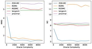
(a) Sampling accuracy against oracle complexity. For any fixed oracle complexity, ZOD-MC has the least error. Note diffusion based methods do not have an initialization and thus curves don’t start at the same $y$ coordinate.

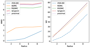
(b) Sampling accuracy against how separated modes are. ZOD-MC is the least sensitive to mode separation. The oracle complexity is fixed, independent of how modes are separated.

Matched Oracle Complexity. We modify a $2$D Gaussian mixture example frequently considered in the literature to make it more challenging, by making its modes unbalanced with non-isotropic variances, resulting in a highly asymmetrical, multi-modal problem. We include the full details of the parameters in Appendix B. We fix the same oracle complexity (total number of 0^th and 1^st order $V$ queries) for different methods, and show the generated samples in Figure 2. Note matching oracle complexity puts our method at a disadvantage, since other techniques require querying the gradient, which results in more function evaluations. Despite this, we see in Figure 1(a) that our method achieves both the lowest MMD and $W_{2}$ using the least number of oracle complexity.

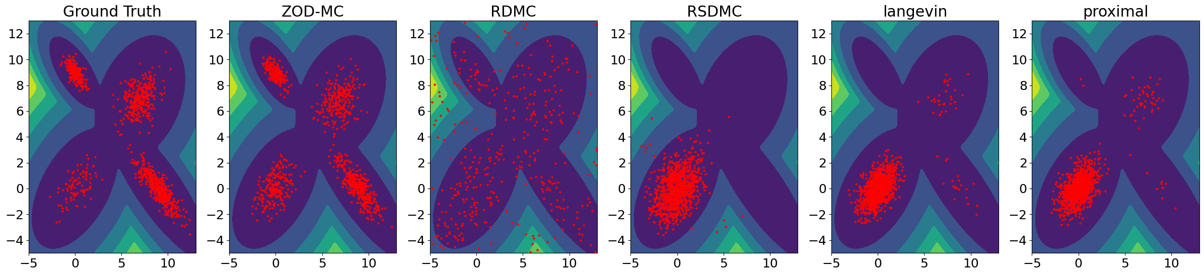
Figure 2: Sampling from asymmetric, unbalanced Gaussian Mixture. All diffusion-based methods (ZOD-MC, RDMC, RSDMC) use $2100$ oracles per score evaluation. Langevin and the proximal sampler are set to use the same total amount of oracles as diffusion based methods. While other methods suffer from metastability, ZOD-MC correctly samples all modes.

Robustness Against Mode Separation. Now let’s further separate the modes in the mixture to investigate the robustness of our method to increasing nonconvexity/metastability. More precisely, we multiply the mean of each mode by a constant factor $R$; doing so increases the barriers between the modes and exponentially worsens the isoperimetric properties of the target distribution [32]. Figure 1(b) shows our method is the most insensitive to mode separation. Being the only one that can successfully sample from all modes, as observed in Figure 3, ZOD-MC suffers less from metastability. Note there is still some dependence on mode separation due to the $x_{k}$ dependence in the complexity bound in Corollary 1.

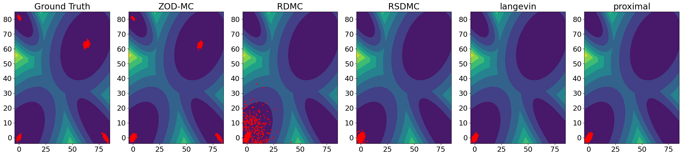
Figure 3: Gaussian Mixture with further separated modes (R=9). ZOD-MC can overcome strengthened metastability and sample from every mode, while other methods are stuck at the mode at the origin, where every method is initialized.

Discontinuous Potentials. The use of zeroth-order queries allows ZOD-MC to solve problems that would be completely infeasible to first order methods. To demonstrate this, we modify the potential by considering $V(x)+U(x)$ where $U$ is a discontinuous function given by $U(x)=8\lfloor\left\lVert x\right\rVert\rfloor\mathbbm{1}_{\{5<\left\lVert x\right\rVert<10\}}$ This creates an annulus of much lower probability and a strong potential barrier. In the original problem, the mode centered at the origin was chosen to have the smallest weight ($0.1$), but adding this discontinuity significantly changes the problem. As observed in Figure 4, our method is still able to correctly sample from the target distribution, while other methods not only continue to suffer from metastability but also fail to see the discontinuities.

We quantitatively evaluate the sampling accuracy by using rejection sampling (slow but unbiased) to obtain ground truth samples, and then compute MMD and $W_{2}$. See Appendix B.2 for details.

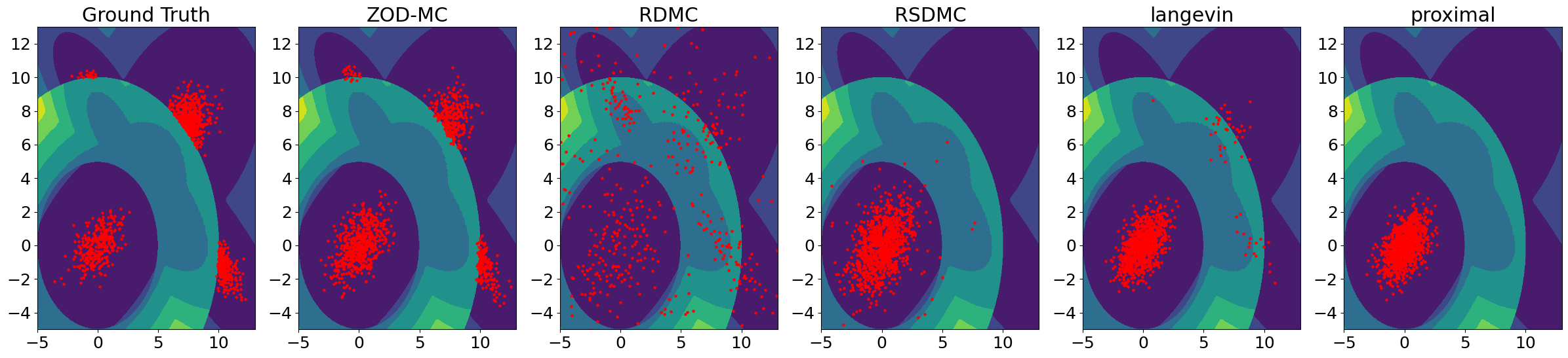
Figure 4: Generated samples for discontinuous Gaussian Mixture. Our method can recover the target distribution even under the presence of discontinuities. The same oracle complexity is again used in each method, $3100$ per score evaluation in diffusion-based approaches.

4.2 Results of Müller Brown Potential

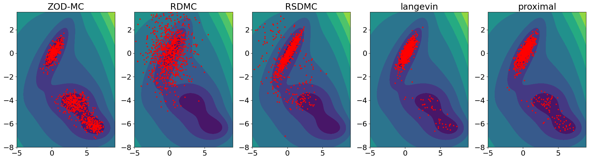
Figure 5: Generated samples for the Müller Brown potential. We overlay the generated samples on top of the level curves of $V(x)$. All methods use $1100$ oracles.

The Müller Brown potential is a toy model for molecular dynamics. Its highly nonlinear potential has 3 modes despite of being the sum of 4 exponentials. The original version has 2 of its modes corresponding to negligible probabilities when compared to the 3rd, which is not good to visualization and comparison across different methods, and we thus consider a balanced version [25] and further translate and dilate $x$ and $y$ so that one of the modes is centered near the origin. The details of the potential can be found in Appendix B.4. Our method is the only one that can correctly sample from all $3$ modes as observed in Figure 5 (note they are leveled).

Appendix A Proofs

A.1 Properties of the OU-Process

In this section, we introduce and prove some useful properties of the OU-process. Throughout this section, we denote $\{X_{t}\}_{t\geq 0}$ as the solution of (1) with $p_{t}\coloneqq\mathrm{Law}(X_{t})$. For any $s,t>0$, $p_{t|s}$ denotes the conditional probability measure of $X_{t}$ given the value of $X_{s}$.

Proposition 3.

(Decay along the OU-Process) Let $\{X_{t}\}_{t\geq 0}$ be the solution of (1) with $p_{t}\coloneqq\mathrm{Law}(X_{t})$. Assume that the initial distribution $p$ satisfies Assumption 1. Then we have

$$W_{2}(p_{t},p)^{2} \leq(1-e^{-t})^{2}\mathrm{m}_{2}^{2}+(1-e^{-2t})d,$$ (13)

$$\text{and}\quad\text{KL}(p_{t}|\gamma^{d}) \leq\frac{1}{2}\frac{e^{-4t}}{1-e^{-2t}}d+\frac{1}{2}e^{-2t}\mathrm{m}_{2}^{2}.$$ (14)

Proof of Proposition 3.

The proof for (13) is based on the fact that the solution to (1) can be represented by

$$X_{t}=e^{-t}X_{0}+\sqrt{1-e^{-2t}}Z,\quad\forall\ t\geq 0.$$ (15)

We have

$$W_{2}(p_{t},p)^{2} \leq\mathbb{E}\big{[}\left\lVert X_{t}-X_{0}\right\rVert^{2}\big{]}\leq\mathbb{E}_{(X_{0},Z)\sim p\otimes\gamma^{d}}\big{[}\lVert(e^{-t}-1)X_{0}+\sqrt{1-e^{-2t}}Z\rVert^{2}\big{]}$$

$$=(1-e^{-t})^{2}\mathrm{m}_{2}^{2}+(1-e^{-2t})d.$$

Next, to prove (14), we have

$$\text{KL}(p_{t}|\gamma^{d}) =\text{KL}(\int p_{t|0}(\cdot|y)p(\mathrm{d}y)|\gamma^{d}(\cdot))\leq\int\text{KL}(p_{t|0}(\cdot|y)|\gamma^{d})p(\mathrm{d}y),$$

where the inequality follows from the convexity of KL divergence. According to (15), $p_{t|0}(\cdot|y)$ is a Gaussian measure with mean $e^{-t}y$ and covariance matrix $(1-e^{-2t})I_{d}$. According to [28], we have

$$\text{KL}(p_{t|0}(\cdot|y)|\gamma^{d})=\text{KL}(\mathcal{N}(e^{-t}y,(1-e^{-2t)I_{d}})|\mathcal{N}(0,I_{d}))=\frac{1}{2}\big{(}-d\ln(1-e^{-2t})-e^{-2t}d+e^{-2t}\left\lVert y\right\rVert^{2}\big{)}.$$

As a result, we get

$$\text{KL}(p_{t}|\gamma^{d}) \leq-\frac{d}{2}\ln(1-e^{-2t})-\frac{d}{2}e^{-2t}+\frac{1}{2}e^{-2t}\int\left\lVert y\right\rVert^{2}p(\mathrm{d}y)\leq\frac{e^{-4t}}{2(1-e^{-2t})}d+\frac{1}{2}e^{-2t}\mathrm{m}_{2}^{2},$$

where the last inequality follows from the fact that $\ln(1+x)\leq x$ for all $x>0$. ∎

Proposition 4.

(Stochastic Dynamics along the OU-Process) Let $\{X_{t}\}_{t\geq 0}$ be the solution of (1). Define $m_{t}(X_{t})\coloneqq\mathbb{E}_{X_{0}\sim p_{0|t}(\cdot|X_{t})}[X_{0}]$ and $\Sigma_{t}(X_{t})\coloneqq\mathrm{Cov}_{X_{0}\sim p_{0|t}(\cdot|X_{t})}(X_{0})=\mathbb{E}_{X_{0}\sim p_{0|t}(\cdot|X_{t})}[(X_{0}-m_{t}(X_{t}))^{\otimes 2}]$. Then we have for all $t\geq 0$,

$$\frac{\mathrm{d}}{\mathrm{d}t}\mathbb{E}\big{[}\Sigma_{t}(X_{t})\big{]}=\frac{2e^{-2t}}{(1-e^{-2t})^{2}}\mathbb{E}\big{[}\Sigma_{t}(X_{t})^{2}\big{]}.$$

The above proposition is known in stochastic localization literatures [6] and diffusion model literatures [2]. We present its proof for the sake of completeness.

Proof of Proposition 4.

For any $T>0$, from (15), we have the conditional distribution

$$p_{0|t}(\mathrm{d}x|X_{t})\propto\exp\big{(}-\frac{1}{2}\frac{\lVert X_{t}-e^{-t}x\rVert^{2}}{1-e^{-2t}}\big{)}p(\mathrm{d}x),$$

where $\{X_{t}\}_{0\leq t\leq T}$ is the solution of (1). Noticing that the solution of (2), $\{\bar{X}_{t}\}_{0\leq t\leq T}$ is the reverse process of $\{X_{t}\}_{0\leq t\leq T}$ and it satisfies $\bar{X}_{t}=X_{T-t}$ in distribution for all $t\in[0,T]$. Therefore, it suffices to study

$$q_{0|t}(\mathrm{d}x|\bar{X}_{t}) \coloneqq Z^{-1}\exp\big{(}-\frac{1}{2}\frac{\lVert\bar{X}_{t}-e^{-(T-t)}x\rVert^{2}}{1-e^{-2(T-t)}}\big{)}p(\mathrm{d}x)$$

$$=Z_{t}^{-1}\exp\big{(}-\frac{1}{2}\frac{e^{-2(T-t)}}{1-e^{-2(T-t)}}\lVert x\rVert^{2}+\frac{e^{-(T-t)}}{1-e^{-2(T-t)}}\langle x,\bar{X}_{t}\rangle\big{)}p(\mathrm{d}x)$$

$$\coloneqq Z_{t}^{-1}\exp(h_{t}(x))p(\mathrm{d}x),$$ (16)

where the normalization constant $Z_{t}=\int_{\mathbb{R}^{d}}\exp(h_{t}(x))p(\mathrm{d}x)$. We have $q_{0|t}(\mathrm{d}x|\bar{X}_{t})=p_{0|T-t}(\mathrm{d}x|X_{T-t})$ in distribution for all $t\in[0,T]$ and

$$\bar{m}_{t}(\bar{X}_{t}) \coloneqq\mathbb{E}_{X_{0}\sim q_{0|t}(\cdot|\bar{X}_{t})}[X_{0}]=\mathbb{E}_{X_{0}\sim p_{0|T-t}(\cdot|X_{T-t})}[X_{0}]=m_{T-t}(X_{T-t}),$$ (17)

$$\bar{\Sigma}_{t}(\bar{X}_{t}) \coloneqq\mathrm{Cov}_{X_{0}\sim q_{0|t}(\cdot|\bar{X}_{t})}(X_{0})=\mathrm{Cov}_{X_{0}\sim p_{0|T-t}(\cdot|{X}_{T-t})}(X_{0})=\Sigma_{T-t}(X_{T-t}).$$ (18)

where the above two identities hold in distribution. For simplicity, we denote $\sigma_{t}=\sqrt{1-e^{-2t}}$. Then $h_{t}(x)=-\frac{1}{2}(\sigma_{T-t}^{-2}-1)\lVert x\rVert^{2}+\sigma_{T-t}^{-1}\sqrt{\sigma_{T-t}^{-2}-1}\langle x,\bar{X}_{t}\rangle$ is a stochastic process linearly depending on $\{\bar{X}_{t}\}_{t\geq 0}$. The conditional measure $\{q_{0|t}(x|\bar{X}_{t})\}_{t\geq 0}$ is a measure-valued stochastic process, its dynamics can be studied by applying Itô’s formula. First we have

$$\mathrm{d}h_{t}(x)=\sigma_{T-t}^{-3}\dot{\sigma}_{T-t}\left\lVert x\right\rVert^{2}\mathrm{d}t+(\sigma_{T-t}^{-2}-1)^{-\frac{1}{2}}\big{(}-2\sigma_{T-t}^{-4}\dot{\sigma}_{T-t}+\sigma_{T-t}^{-2}\dot{\sigma}_{T-t}\big{)}\langle x,\bar{X}_{t}\rangle\mathrm{d}t$$

$$\qquad\quad\quad+\sigma_{T-t}^{-1}(\sigma_{T-t}^{-2}-1)^{\frac{1}{2}}\langle x,\mathrm{d}\bar{X}_{t}\rangle,$$ (19)

$$\mathrm{d}[h(x),h(x)]_{t}=\sigma_{T-t}^{-2}(\sigma_{T-t}^{-2}-1)\left\lVert x\right\rVert^{2}\mathrm{d}[\bar{X},\bar{X}]_{t},$$ (20)

Since $\{\bar{X}_{t}\}_{0\leq t\leq T}$ solves (2), according to Lemma 1, it satisfies that

$$\mathrm{d}\bar{X}_{t} =\big{(}\bar{X_{t}}+2\mathbb{E}_{x\sim p_{0|T-t}(\cdot|\bar{X}_{t})}\big{[}\frac{e^{-(T-t)}x-\bar{X}_{t}}{1-e^{-2(T-t)}}\big{]}\big{)}\mathrm{d}t+\sqrt{2}\mathrm{d}\bar{B}_{t}$$

$$=\big{(}-\sigma_{T-t}^{-2}(2-\sigma_{T-t}^{-2})\bar{X}_{t}+2(1-\sigma_{T-t}^{2})^{\frac{1}{2}}\bar{m}_{t}(\bar{X}_{t})\big{)}\mathrm{d}t+\sqrt{2}\mathrm{d}\bar{B}_{t}.$$ (21)

Based on (19), (20) and (21), we have

$$\mathrm{d}Z_{t} =\int_{\mathbb{R}^{d}}\exp\big{(}h_{t}(x)\big{)}\big{(}\mathrm{d}h_{t}(x)+\frac{1}{2}\mathrm{d}[h(x),h(x)]_{t}\big{)}p(\mathrm{d}x)$$

$$=\big{(}\sigma_{T-t}^{-3}\dot{\sigma}_{T-t}+\sigma_{T-t}^{-2}(\sigma_{T-t}^{-2}-1)\big{)}\mathbb{E}_{q_{0|t}(\cdot|\bar{X}_{t})}\big{[}\left\lVert x\right\rVert^{2}\big{]}Z_{t}\mathrm{d}t$$

$$\quad+(\sigma_{T-t}^{-2}-1)^{-\frac{1}{2}}\big{(}-2\sigma_{T-t}^{-4}\dot{\sigma}_{T-t}+\sigma_{T-t}^{-2}\dot{\sigma}_{T-t}\big{)}\langle\bar{m}_{t}(\bar{X}_{t}),\bar{X}_{t}\rangle Z_{t}\mathrm{d}t$$

$$\quad+\sigma_{T-t}^{-1}(\sigma_{T-t}^{-2}-1)^{\frac{1}{2}}\langle\bar{m}_{t}(\bar{X}_{t}),\mathrm{d}\bar{X}_{t}\rangle Z_{t},$$

$$\text{and}\quad\mathrm{d}\ln Z_{t} =Z_{t}^{-1}\mathrm{d}Z_{t}-\frac{1}{2}Z_{t}^{-2}\mathrm{d}[Z,Z]_{t}$$

$$=\big{(}\sigma_{T-t}^{-3}\dot{\sigma}_{T-t}+\sigma_{T-t}^{-2}(\sigma_{T-t}^{-2}-1)\big{)}\mathbb{E}_{q_{0|t}(\cdot|\bar{X}_{t})}\big{[}\left\lVert x\right\rVert^{2}\big{]}\mathrm{d}t$$

$$\quad+(\sigma_{T-t}^{-2}-1)^{-\frac{1}{2}}\big{(}-2\sigma_{T-t}^{-4}\dot{\sigma}_{T-t}+\sigma_{T-t}^{-2}\dot{\sigma}_{T-t}\big{)}\langle\bar{m}_{t}(\bar{X}_{t}),\bar{X}_{t}\rangle\mathrm{d}t$$

$$\quad+\sigma_{T-t}^{-1}(\sigma_{T-t}^{-2}-1)^{\frac{1}{2}}\langle\bar{m}_{t}(\bar{X}_{t}),\mathrm{d}\bar{X}_{t}\rangle$$

$$\quad+\sigma_{T-t}^{-2}(\sigma_{T-t}^{-2}-1)\left\lVert\bar{m}_{t}(\bar{X}_{t})\right\rVert^{2}\mathrm{d}t.$$ (22)

If we define $R_{t}(x_{t})=\frac{q_{0|t}(\mathrm{d}x|\bar{X}_{t})}{p(\mathrm{d}x)}=Z_{t}^{-1}\exp(h_{t}(x))$, then apply Itô’s formula again and we have

$$\mathrm{d}R_{t}(X_{t}) =\mathrm{d}\exp\big{(}\ln R_{t}(X_{t})\big{)}$$

$$=R_{t}(X_{t})\mathrm{d}\big{(}\ln R_{t}(X_{t})\big{)}+\frac{1}{2}R_{t}(X_{t})\mathrm{d}\big{[}\ln R_{t}(X_{t}),\ln R_{t}(X_{t})\big{]}$$

$$=R_{t}(X_{t})\mathrm{d}h_{t}(x)-R_{t}(X_{t})\mathrm{d}\ln Z_{t}+\frac{1}{2}R_{t}(X_{t})\mathrm{d}\big{[}h_{t}(x)-\ln Z_{t},h_{t}(x)-\ln Z_{t}\big{]}.$$ (23)

Now combine the results in (19), (20), (22) and (23), we can derive the differential equation of $m_{t}(X_{t})$:

$$\mathrm{d}m_{t}(X_{t}) =\mathrm{d}\int_{\mathbb{R}^{d}}xR_{t}(X_{t})p(\mathrm{d}x)$$

$$=\int_{\mathbb{R}^{d}}x\big{(}\mathrm{d}h_{t}(x)-d\ln Z_{t}+\frac{1}{2}\mathrm{d}\big{[}h_{t}(x)-\ln Z_{t},h_{t}(x)-\ln Z_{t}\big{]}\big{)}p_{0|t}(\mathrm{d}x|X_{t})$$

$$=\sigma_{T-t}^{-3}\dot{\sigma}_{T-t}\mathbb{E}_{q_{0|t}(\cdot|\bar{X}_{t})}\big{[}\left\lVert x\right\rVert^{2}x\big{]}\mathrm{d}t$$

$$\quad+(\sigma_{T-t}^{-2}-1)^{-\frac{1}{2}}\big{(}-2\sigma_{T-t}^{-4}\dot{\sigma}_{T-t}+\sigma_{T-t}^{-2}\dot{\sigma}_{T-t}\big{)}\mathbb{E}_{q_{0|t}(\cdot|\bar{X}_{t})}\big{[}x^{\otimes 2}\big{]}\bar{X}_{t}\mathrm{d}t$$

$$\quad+\sigma_{T-t}^{-1}(\sigma_{T-t}^{-2}-1)^{\frac{1}{2}}\mathbb{E}_{q_{0|t}(\cdot|\bar{X}_{t})}\big{[}x^{\otimes 2}\mathrm{d}\bar{X}_{t}\big{]}$$

$$\quad-\sigma_{T-t}^{-3}\dot{\sigma}_{T-t}\mathbb{E}_{q_{0|t}(\cdot|\bar{X}_{t})}\big{[}\left\lVert x\right\rVert^{2}\big{]}\bar{m}_{t}(\bar{X}_{t})\mathrm{d}t$$

$$\quad-(\sigma_{T-t}^{-2}-1)^{-\frac{1}{2}}\big{(}-2\sigma_{T-t}^{-4}\dot{\sigma}_{T-t}+\sigma_{T-t}^{-2}\dot{\sigma}_{T-t}\big{)}\bar{m}_{t}(\bar{X}_{t})^{\otimes 2}\bar{X}_{t}\mathrm{d}t$$

$$\quad-\sigma_{T-t}^{-1}(\sigma_{T-t}^{-2}-1)^{\frac{1}{2}}\bar{m}_{t}(\bar{X}_{t})^{\otimes 2}\mathrm{d}\bar{X}_{t}$$

$$\quad-\sigma_{T-t}^{-2}(\sigma_{T-t}^{-2}-1)\left\lVert\bar{m}_{t}(\bar{X}_{t})\right\rVert^{2}\bar{m}_{t}(\bar{X}_{t})\mathrm{d}t$$

$$\quad+\sigma_{T-t}^{-2}(\sigma_{T-t}^{-2}-1)\mathbb{E}_{q_{0|t}(\cdot|\bar{X}_{t})}\big{[}\lVert x-\bar{m}_{t}(\bar{X}_{t})\rVert^{2}x\big{]}\mathrm{d}t.$$ (24)

Utilize (21) and the definition of $\sigma_{t}$, all terms with factor $\mathrm{d}t$ in the above equation cancel and (24) can be simplified as

$$\mathrm{d}\bar{m}_{t}(\bar{X}_{t}) =\frac{\sqrt{2}e^{-(T-t)}}{1-e^{-2(T-t)}}\mathbb{E}_{q_{0|t}(\cdot|\bar{X}_{t})}\big{[}x\otimes(x-\bar{m}_{t}(\bar{X}_{t}))\mathrm{d}B_{t}\big{]}$$

$$=\frac{\sqrt{2}e^{-(T-t)}}{1-e^{-2(T-t)}}\bar{\Sigma}_{t}(\bar{X}_{t})\mathrm{d}\bar{B}_{t}.$$ (25)

Last, we derive the differential equation that $\mathbb{E}_{X_{t}\sim p_{t}}\big{[}\Sigma_{t}(X_{t})\big{]}$ satisfies. Let $f(t)\coloneqq\mathbb{E}_{X_{t}\sim p_{t}}\big{[}\Sigma_{t}(X_{t})\big{]}$ and $g(t)\coloneqq\mathbb{E}_{X_{t}\sim p_{t}}\big{[}\Sigma_{t}(X_{t})^{2}\big{]}$ be two deterministic functions on $[0,T]$. According to (18) and (25), we have

$$\frac{\mathrm{d}}{\mathrm{d}t}f(T-t) =\frac{\mathrm{d}}{\mathrm{d}t}\mathbb{E}_{X_{T-t}\sim p_{T-t}}\left[\Sigma_{T-t}(X_{T-t})\right]$$

$$=\frac{\mathrm{d}}{\mathrm{d}t}\mathbb{E}_{\bar{X}_{t}\sim p_{T-t}}\big{[}\bar{\Sigma}_{t}(\bar{X}_{t})\big{]}$$

$$=\frac{\mathrm{d}}{\mathrm{d}t}\mathbb{E}_{\bar{X}_{t}\sim p_{T-t}}\big{[}\mathbb{E}_{q_{0|t}(\cdot|\bar{X}_{t})}[x^{\otimes}2]-\bar{m}_{t}(\bar{X}_{t})^{\otimes 2}\big{]}$$

$$=\frac{\mathrm{d}}{\mathrm{d}t}\mathbb{E}_{x\sim p}[x^{\otimes}2]-\frac{\mathrm{d}}{\mathrm{d}t}\mathbb{E}_{X_{t}\sim p_{t}}\big{[}\bar{m}_{t}(\bar{X}_{t})^{\otimes 2}\big{]}$$

$$=-\frac{2e^{-2(T-t)}}{(1-e^{-2(T-t)})^{2}}\mathbb{E}_{\bar{X}_{t}\sim p_{T-t}}\big{[}\bar{\Sigma}_{t}(\bar{X}_{t})^{2}\big{]}$$

$$=-\frac{2e^{-2(T-t)}}{(1-e^{-2(T-t)})^{2}}g(T-t).$$

where the last inequality follows from the Itô isometry. Proposition 4 is then proved by reverse the time in $f$ and $g$. ∎

A.2 Proofs of Section 3.1

Proof of Lemma 1.

Based on (15), we have $p_{t}=(e^{-t})_{\#p}\ast(\sqrt{1-e^{-2t}})_{\#\gamma^{d}}$ where $(e^{-t})_{\#p}$ is the pushforward measure of $p$ via map $x\in\mathbb{R}^{d}\mapsto e^{-t}x$ and $(\sqrt{1-e^{-2t}})_{\#\gamma^{d}}$ is the pushforward measure of $\gamma^{d}$ via map $x\in\mathbb{R}^{d}\mapsto\sqrt{1-e^{-2t}}x\in\mathbb{R}^{d}$. The pushforward measures $(e^{-t})_{\#p}$ and $(\sqrt{1-e^{-2t}})_{\#\gamma^{d}}$ can be written as

$$(e^{-t})_{\#p}(\mathrm{d}x) =e^{td}p(e^{t}\mathrm{d}x)\quad\text{and}$$

$$(\sqrt{1-e^{-2t}})_{\#\gamma^{d}}(\mathrm{d}x) =\big{(}2\pi(1-e^{-2t})\big{)}^{-\frac{d}{2}}\exp\big{(}-\frac{\left\lVert x\right\rVert^{2}}{2(1-e^{-2t})}\big{)}\mathrm{d}x,$$

respectively. Therefore the score function $\nabla\ln p_{t}(x)$ can be written as

$$\nabla\ln p_{t}(x) =p_{t}(x)^{-1}e^{td}\big{(}2\pi(1-e^{-2t})\big{)}^{-\frac{d}{2}}\nabla_{x}\int\exp\big{(}-\frac{\left\lVert x-z\right\rVert^{2}}{2(1-e^{-2t})}\big{)}p(e^{t}\mathrm{d}z)$$

$$=p_{t}(x)^{-1}\big{(}2\pi(1-e^{-2t})\big{)}^{-\frac{d}{2}}\nabla_{x}\int\exp\big{(}-\frac{\left\lVert x-e^{-t}z\right\rVert^{2}}{2(1-e^{-2t})}\big{)}p(\mathrm{d}z)$$

$$=\int\frac{x-e^{-t}z}{1-e^{-2t}}\frac{p_{t|0}(x|z)p(\mathrm{d}z)}{p_{t}(x)}$$

$$=\int\frac{x-e^{-t}z}{1-e^{-2t}}p_{0|t}(\mathrm{d}z|x),$$

where the last step follows from the Bayesian rule and

$$p_{0|t}(\cdot|x)\propto p_{t|0}(x|\cdot)p(\cdot)\propto\exp\big{(}-V(\cdot)-\frac{1}{2}\frac{\left\lVert x-e^{-t}\cdot\right\rVert^{2}}{1-e^{-2t}}\big{)}.$$

∎

A.3 Proofs of Section 3.2

Proof of Proposition 1.

With the score estimator given in Algorithm 2, we have

$$\mathbb{E}_{x\sim p_{t}}\big{[}\left\lVert\nabla\ln p_{t}(x)-s(t,x)\right\rVert^{2}\big{]} =\mathbb{E}_{x\sim p_{t}}\big{[}\lVert\nabla\ln p_{t}(x)-\frac{1}{n(t)}\sum_{i=1}^{n(t)}\frac{e^{-t}z_{t,i}-x}{1-e^{-2t}}\rVert^{2}\big{]}$$

$$=\mathbb{E}_{x\sim p_{t}}\big{[}\lVert\nabla\ln p_{t}(x)-\frac{1}{n(t)}\sum_{i=1}^{n(t)}\frac{e^{-t}x_{t,i}-x}{1-e^{-2t}}+\frac{1}{n(t)}\sum_{i=1}^{n(t)}\frac{x_{t,i}-z_{t,i}}{1-e^{-2t}}\rVert^{2}\big{]},$$

where $\{x_{t,i}\}_{i=1}^{n(t)}$ is a sequence of i.i.d. samples following $p_{0|t}(\cdot|x)$ that are chosen such that $\mathbb{E}[\left\lVert x_{t,i}-z_{t,i}\right\rVert^{2}]=W_{2}(p_{t},\mathrm{Law}(z_{t,i}))$ for all $t>0$ and $i=1,2,\cdots,n(t)$. Based on Lemma 1, $\{\frac{e^{-t}x_{t,i}-x}{1-e^{-2t}}\}_{i=1}^{n(t)}$ is a sequence of unbiased i.i.d. Monte Carlo estimator of $\nabla\ln p_{t}(x)$ for all $t>0$ and $x\in\mathbb{R}^{d}$. Therefore, we get

$$\quad\mathbb{E}_{x\sim p_{t}}\big{[}\left\lVert\nabla\ln p_{t}(x)-s(t,x)\right\rVert^{2}\big{]}$$

$$=\mathbb{E}_{x\sim p_{t}}\big{[}\lVert\nabla\ln p_{t}(x)-\frac{1}{n(t)}\sum_{i=1}^{n(t)}\frac{e^{-t}x_{t,i}-x}{1-e^{-2t}}+\rVert^{2}\big{]}+\mathbb{E}\big{[}\lVert\frac{1}{n(t)}\sum_{i=1}^{n(t)}\frac{x_{t,i}-z_{t,i}}{1-e^{-2t}}\rVert^{2}\big{]}$$

$$=\underbrace{\frac{1}{n(t)^{2}}\sum_{i=1}^{n(t)}\mathbb{E}_{x\sim p_{t}}\big{[}\lVert\frac{e^{-t}x_{t,i}-x}{1-e^{-2t}}-\mathbb{E}_{x_{t,i}\sim p_{0|t}(\cdot|x)}[\frac{e^{-t}x_{t,i}-x}{1-e^{-2t}}]\rVert^{2}]\big{]}}_{N_{1}}$$

$$\quad+\underbrace{\frac{e^{-2t}}{(1-e^{-2t})^{2}}\frac{1}{n(t)^{2}}\sum_{i,j=1}^{n(t)}\mathbb{E}\big{[}\langle x_{t,i}-z_{t,i},x_{t,j}-z_{t,j}\rangle\big{]}}_{N_{2}}.$$

The first term in the above equation, $N_{1}$, is related to the covariance of $p_{0|t}(\cdot|X_{t})$, which is studied in Proposition 4. We have

$$N_{1} =\frac{e^{-2t}}{(1-e^{-2t})^{2}}\frac{1}{n(t)^{2}}\sum_{i=1}^{n(t)}\mathbb{E}_{x\sim p_{t}}\big{[}\text{trace}\big{(}\mathrm{Cov}_{x_{t,i}\sim p_{0|t}(\cdot|x)}(x_{t,i})\big{)}\big{]}$$

$$=\frac{e^{-2t}}{(1-e^{-2t})^{2}}\frac{1}{n(t)}\mathbb{E}_{x\sim p_{t}}\big{[}\text{trace}\big{(}\Sigma_{t}(x)\big{)}\big{]}$$

$$\leq\frac{e^{-2t}}{(1-e^{-2t})^{2}}\frac{1}{n(t)}\mathbb{E}_{x\sim\gamma^{d}}\big{[}\text{trace}\big{(}\Sigma_{\infty}(x)\big{)}\big{]}$$

$$=\frac{e^{-2t}}{(1-e^{-2t})^{2}}\frac{1}{n(t)}\mathrm{Cov}_{p}(x),$$

where the inequality follows from Proposition 4 indicating that $t\mapsto\mathbb{E}_{x\sim p_{t}}\big{[}\text{trace}\big{(}\Sigma_{t}(x)\big{)}\big{]}$ is a increasing function.

The second term $N_{2}$ characterize the bias from the Monte Carlo samples and the bias can be measured by the Wasserstein-2 distance:

$$N_{2} \leq\frac{e^{-2t}}{(1-e^{-2t})^{2}}\frac{1}{n(t)^{2}}\sum_{i,j=1}^{n(t)}\mathbb{E}\big{[}\lVert x_{t,i}-z_{t,i}\rVert^{2}\big{]}^{\frac{1}{2}}\mathbb{E}\big{[}\lVert x_{t,j}-z_{t,j}\rVert^{2}\big{]}^{\frac{1}{2}}$$

$$=\frac{e^{-2t}}{(1-e^{-2t})^{2}}\frac{1}{n(t)^{2}}\sum_{i,j=1}^{n(t)}W_{2}(\mathrm{Law}(z_{t,i}),p_{0|t}(\cdot|x))W_{2}(\mathrm{Law}(z_{t,j}),p_{0|t}(\cdot|x))$$

$$\leq\frac{e^{-2t}}{(1-e^{-2t})^{2}}{\delta(t)^{2}}.$$

(4) follows from the estimation on $N_{1}$ and $N_{2}$. ∎

A.4 Proof of Theorem 1

In this section, we introduce the proof of our main convergence results, Theorem 1. Recall that in the convergence result in Theorem 1, three types of errors appear in the upper bound: the initialization error, the discretization error and the score estimation error. Our proof compares the trajectory of $\{\tilde{X}_{t}\}_{0\leq t\leq T}$ that solves (9) and the trajectory of $\{\bar{X}_{t}\}_{0\leq t\leq T}$ that solves (2). We denote the path measures of $\{\bar{X}_{t}\}_{0\leq t\leq T}$ and $\{\tilde{X}_{t}\}_{0\leq t\leq T}$ by ${P}^{p_{T}}$, and ${Q}^{\gamma^{d}}$, respectively. Next, we introduce a high level idea on how the three types of errors are handled .

1. Initialization error: the initialization error comes from the comparison between $\{\tilde{X}_{t}\}_{0\leq t\leq T}$ and $\{\tilde{X}_{t}^{p_{T}}\}_{0\leq t\leq T}$. To characterize this error, we introduce the intermediate process $\{\tilde{X}_{t}^{p_{T}}\}_{0\leq t\leq T}$

   $$\mathrm{d}\tilde{X}_{t}^{p_{T}}=(\tilde{X}_{t}^{p_{T}}+2s({T-t_{k}},\tilde{X}_{t_{k}}^{p_{T}})\mathrm{d}t+\sqrt{2}\mathrm{d}\tilde{B}_{t},\quad\tilde{X}_{0}\sim p_{T},\ t\in[t_{k},t_{k+1}),$$ (26)

   in (26) and denote the path measure of $\{\tilde{X}_{t}^{p_{T}}\}_{0\leq t\leq T}$ by ${Q}^{p_{T}}$. Both processes are driven by the estimated scores and only the initial conditions are different. We factor out the initialization error from $\text{KL}(p_{\delta}|q_{t_{N}})$ by the following argument:

   $$\text{KL}(p_{\delta}|q_{t_{N}}) =\text{KL}(p_{\delta}|q_{T-\delta})$$

   $$\leq\int\ln\frac{\mathrm{d}P^{p^{T}}}{\mathrm{d}Q^{\gamma^{d}}}\mathrm{d}P^{p_{T}}=\int\ln\big{(}\frac{\mathrm{d}P^{p^{T}}}{\mathrm{d}Q^{p_{T}}}\frac{\mathrm{d}Q^{p_{T}}}{\mathrm{d}Q^{\gamma^{d}}}\big{)}\mathrm{d}P^{p_{T}}$$

   $$=\text{KL}(P^{p_{T}}|Q^{p_{T}})+\int\ln\frac{\mathrm{d}Q^{p_{T}}}{\mathrm{d}Q^{\gamma^{d}}}\mathrm{d}P^{p_{T}}$$

   $$=\text{KL}(P^{p_{T}}|Q^{p_{T}})+\text{KL}(p_{T}|\gamma^{d}),$$

   where the inequality follows from the data processing inequality and the last identity follows from the fact that $\frac{\mathrm{d}Q^{p_{T}}}{\mathrm{d}Q^{\gamma^{d}}}=\frac{\mathrm{d}Q^{p_{T}}_{0}}{\mathrm{d}Q^{\gamma^{d}}_{0}}=\frac{\mathrm{d}p_{T}}{\mathrm{d}\gamma^{d}}$, which is true because the processes $\{\tilde{X}_{t}\}_{0\leq t\leq T}$ and $\{\tilde{X}_{t}^{p_{T}}\}_{0\leq t\leq T}$ have the same transition kernel function. $\text{KL}(p_{T}|\gamma^{d})$ is the initialization error and it is bounded based on (14) in Proposition 3.

2. Discretization error: the dicretization error arises from the evaluations of the scores at the discrete times. We factor out the discretization error from the $\text{KL}(P^{p_{T}}|Q^{p_{T}})$ via the Girsanov’s Theorem.

   $$\text{KL}(P^{p_{T}}|Q^{p_{T}}) \leq\sum_{k=0}^{N-1}\int_{t_{k}}^{t_{k+1}}\mathbb{E}_{P^{p_{T}}}\big{[}\left\lVert\nabla\ln p_{T-t}(\bar{X}_{t})-s(T-t_{k},\bar{X}_{t_{k}})\right\rVert^{2}\big{]}\mathrm{d}t$$

   $$\lesssim\underbrace{\sum_{k=0}^{N-1}\int_{t_{k}}^{t_{k+1}}\mathbb{E}_{P^{p_{T}}}\big{[}\left\lVert\nabla\ln p_{T-t}(\bar{X}_{t})-\nabla\ln p_{T-t_{k}}(\bar{X}_{t_{k}})\right\rVert^{2}\big{]}\mathrm{d}t}_{\text{discretization error}}$$

   $$\quad+\underbrace{\sum_{k=0}^{N-1}\gamma_{k}\mathbb{E}_{P^{p_{T}}}\big{[}\left\lVert\nabla\ln p_{T-t_{k}}(\bar{X}_{t_{k}})-s(T-t_{k},\bar{X}_{t_{k}})\right\rVert^{2}\big{]}}_{\text{score estimation error}}$$

   We bound the discretization error term in the above equation by checking the dynamical properties of the process $\{\nabla\ln p_{t}(\bar{X}_{t})\}_{0\leq t\leq T}$. Similar approach was used in the analysis of denoising diffusion models, see [2]. For the sake of completeness, we include the proof in Appendix A.7.

3. Score estimation error: as discussed in the discretization error, the score estimation error is the accumulation of the $L^{2}$-error between the true score and score estimator at the time schedules $\{T-t_{k}\}_{k=0}^{N-1}$. In the analysis of denoising diffusion models, [4, 3, 2], it is usually assumed that such a $L^{2}$ score error is small. In this paper, we consider to do sampling via the Reverse OU-process and score estimation. One of our main contribution is that we prove the $L^{2}$ score error can be guaranteed small for the class of Monte Carlo score estimators given in Algorithm 2. The $L^{2}$ score error upper bound is stated in Proposition 1.

Proof of Theorem 1.

First we can decompose $\text{KL}(p_{\delta}|q_{t_{N}})$ into summation of the three types of error.

$$\text{KL}(p_{\delta}|q_{t_{N}}) =\text{KL}(p_{\delta}|q_{T-\delta})$$

$$\leq\int\ln\frac{\mathrm{d}P^{p^{T}}}{\mathrm{d}Q^{\gamma^{d}}}\mathrm{d}P^{p_{T}}=\int\ln\big{(}\frac{\mathrm{d}P^{p^{T}}}{\mathrm{d}Q^{p_{T}}}\frac{\mathrm{d}Q^{p_{T}}}{\mathrm{d}Q^{\gamma^{d}}}\big{)}\mathrm{d}P^{p_{T}}$$

$$=\text{KL}(P^{p_{T}}|Q^{p_{T}})+\int\ln\frac{\mathrm{d}Q^{p_{T}}}{\mathrm{d}Q^{\gamma^{d}}}\mathrm{d}P^{p_{T}}$$

$$=\text{KL}(P^{p_{T}}|Q^{p_{T}})+\text{KL}(p_{T}|\gamma^{d})$$

$$\leq\text{KL}(p_{T}|\gamma^{d})+\sum_{k=0}^{N-1}\int_{t_{k}}^{t_{k+1}}\mathbb{E}_{P^{p_{T}}}\big{[}\left\lVert\nabla\ln p_{T-t}(\bar{X}_{t})-s(T-t_{k},\bar{X}_{t_{k}})\right\rVert^{2}\big{]}\mathrm{d}t$$

$$\lesssim\underbrace{\text{KL}(p_{T}|\gamma^{d})\vphantom{\sum_{k=0}^{N-1}\int_{t_{k}}^{t_{k+1}}\mathbb{E}_{P^{p_{T}}}\big{[}\left\lVert\nabla\ln p_{T-t}(\bar{X}_{t})-\nabla\ln p_{T-t_{k}}(\bar{X}_{t_{k}})\right\rVert^{2}\big{]}\mathrm{d}t}}_{\text{initialization error}}+\underbrace{\sum_{k=0}^{N-1}\int_{t_{k}}^{t_{k+1}}\mathbb{E}_{P^{p_{T}}}\big{[}\left\lVert\nabla\ln p_{T-t}(\bar{X}_{t})-\nabla\ln p_{T-t_{k}}(\bar{X}_{t_{k}})\right\rVert^{2}\big{]}\mathrm{d}t}_{\text{discretization error}}$$

$$\quad+\underbrace{\sum_{k=0}^{N-1}\gamma_{k}\mathbb{E}_{P^{p_{T}}}\big{[}\left\lVert\nabla\ln p_{T-t_{k}}(\bar{X}_{t_{k}})-s(T-t_{k},\bar{X}_{t_{k}})\right\rVert^{2}\big{]}}_{\text{score estimation error}},$$

where the first inequality follows from the data processing inequality. The second inequality follows from [4, Section 5.2]. According to Proposition 3 and the assumption that $T>1$, the initialization error satisfies

$$\text{KL}(p_{T}|\gamma^{d})\leq\frac{1}{2}\frac{e^{-4T}}{1-e^{-2T}}d+\frac{1}{2}e^{-2T}\mathrm{m}_{2}^{2}\lesssim(d+\mathrm{m}_{2}^{2})e^{-2T}.$$ (27)

According to Lemma 2, the discretization error satisfies

$$\quad\sum_{k=0}^{N-1}\int_{t_{k}}^{t_{k+1}}\mathbb{E}_{P^{p_{T}}}\big{[}\left\lVert\nabla\ln p_{T-t}(\bar{X}_{t})-\nabla\ln p_{T-t_{k}}(\bar{X}_{t_{k}})\right\rVert^{2}\big{]}\mathrm{d}t$$

$$\lesssim d\sum_{k=0}^{N}\frac{\gamma_{k}^{2}}{(1-e^{-2(T-t_{k})})^{2}}+\sum_{k=0}^{N}\frac{e^{-2(T-t_{k})}\gamma_{k}}{(1-e^{-2(T-t_{k})})^{2}}\bigg{(}\mathbb{E}\big{[}\text{trace}\big{(}\Sigma_{T-t_{k}}(X_{T-t_{k}})\big{)}\big{]}-\mathbb{E}\big{[}\text{trace}\big{(}\Sigma_{T-t_{k+1}}(X_{T-t_{k+1}})\big{)}\big{]}\bigg{)}.$$ (28)

Reordering the summation in the second term and we have

$$\quad\sum_{k=0}^{N}\frac{e^{-2(T-t_{k})}\gamma_{k}}{(1-e^{-2(T-t_{k})})^{2}}\bigg{(}\mathbb{E}\big{[}\text{trace}\big{(}\Sigma_{T-t_{k}}(X_{T-t_{k}})\big{)}\big{]}-\mathbb{E}\big{[}\text{trace}\big{(}\Sigma_{T-t_{k+1}}(X_{T-t_{k+1}})\big{)}\big{]}\bigg{)}$$

$$\leq\sum_{k=1}^{N-1}\bigg{(}\frac{e^{-2(T-t_{k})}\gamma_{k}}{(1-e^{-2(T-t_{k})})^{2}}-\frac{e^{-2(T-t_{k-1})}\gamma_{k-1}}{(1-e^{-2(T-t_{k-1})})^{2}}\bigg{)}\mathbb{E}\big{[}\text{trace}\big{(}\Sigma_{T-t_{k}}(X_{T-t_{k}})\big{)}\big{]}+\frac{e^{-2T}\gamma_{0}}{(1-e^{-2T})^{2}}\mathbb{E}\big{[}\text{trace}\big{(}\Sigma_{T}(X_{T})\big{)}\big{]}$$

$$\lesssim\sum_{k=1}^{N-1}\frac{\gamma_{k}\gamma_{k-1}^{2}}{(1-e^{-2(T-t_{k})})^{2}(1-e^{-2(T-t_{k-1})})^{2}}\mathbb{E}\big{[}\text{trace}\big{(}\Sigma_{T-t_{k}}(X_{T-t_{k}})\big{)}\big{]}+\frac{e^{-2T}\gamma_{0}}{(1-e^{-2T})^{2}}\mathbb{E}\big{[}\text{trace}\big{(}\Sigma_{T}(X_{T})\big{)}\big{]}.$$ (29)

Recall that $\Sigma_{t}(X_{t})=\mathrm{Cov}(X_{0}|X_{t})$ for all $0\leq t\leq T$. We have

$$\mathbb{E}\big{[}\text{trace}\big{(}\Sigma_{t}(X_{t})\big{)}\big{]} =\mathbb{E}\big{[}\mathrm{Cov}(X_{0}|X_{t})\big{]}\leq\mathbb{E}\big{[}\left\lVert X_{0}\right\rVert^{2}\big{]}\leq\mathbf{m}_{2}^{2},$$ (30)

$$\text{and}\quad\mathbb{E}\big{[}\text{trace}\big{(}\Sigma_{t}(X_{t})\big{)}\big{]} =\mathbb{E}\big{[}\mathrm{Cov}(X_{0}|X_{t})\big{]}=\mathbb{E}\big{[}\mathrm{Cov}(X_{0}-e^{t}X_{t}|X_{t})\big{]}$$

$$\leq\mathbb{E}\big{[}\mathbb{E}\big{[}\left\lVert X_{0}-e^{t}X_{t}\right\rVert^{2}|X_{t}\big{]}\big{]}$$

$$=(e^{2t}-1)d.$$ (31)

where the last identity follows from (15). (31) and (30) implies that $\mathbb{E}\big{[}\text{trace}\big{(}\Sigma_{t}(X_{t})\big{)}\big{]}\lesssim(1-e^{-2t})(d+\mathbf{m}_{2}^{2})$ for all $0\leq t\leq T$. Therefore, from (28) and (29), the overall discretization error can be bounded as

$$\quad\sum_{k=0}^{N-1}\int_{t_{k}}^{t_{k+1}}\mathbb{E}_{P^{p_{T}}}\big{[}\left\lVert\nabla\ln p_{T-t}(\bar{X}_{t})-\nabla\ln p_{T-t_{k}}(\bar{X}_{t_{k}})\right\rVert^{2}\big{]}\mathrm{d}t$$

$$\lesssim\sum_{k=0}^{N-1}\frac{d\gamma_{k}^{2}}{(1-e^{-2(T-t_{k})})^{2}}+\sum_{k=1}^{N-1}\frac{(d+\mathbf{m}_{2}^{2})\gamma_{k}\gamma_{k-1}^{2}}{(1-e^{-2(T-t_{k})})(1-e^{-2(T-t_{k-1})})^{2}}+\frac{\mathbf{m}_{2}^{2}e^{-2T}\gamma_{0}}{(1-e^{-2T})^{2}}.$$ (32)

Last, according to Proposition 1, the score estimation error satisfies

$$\sum_{k=0}^{N-1}\gamma_{k}\mathbb{E}_{P^{p_{T}}}\big{[}\left\lVert\nabla\ln p_{T-t_{k}}(\bar{X}_{t_{k}})-s(T-t_{k},\bar{X}_{t_{k}})\right\rVert^{2}\big{]}\leq\sum_{k=0}^{N-1}\frac{\gamma_{k}e^{-2(T-t_{k})}}{(1-e^{-2(T-t_{k})})^{2}}\bigg{(}\delta(T-t_{k})^{2}+\frac{d}{n(T-t_{k})}\bigg{)},$$ (33)

and (1) follows from (27), (32) and (33). ∎

A.5 Discussion on the Step-size

In this section, we first provide detailed calculations for error bounds of DMC under different choices of step-size. Then we compare our results in Theorem 1 to existing results on convergence of denoising diffusion models.

1. Constant step-size: when $\gamma_{k}=\gamma$ for all $k=0,1,\cdots,N-1$, we have $T-t_{k}=\delta+(N-k)\gamma$ and

   $$\frac{\gamma_{k}}{1-e^{-2(T-t_{k})}}=\left\{\begin{aligned} &\Theta(\gamma),\quad&\text{if }T-t_{k}>1,\\ &\Theta(\frac{\gamma}{T-t_{k}}),\quad&\text{if }T-t_{k}<1.\end{aligned}\right.$$

   Therefore

   $$\quad\sum_{k=1}^{N-1}\frac{(d+\mathbf{m}_{2}^{2})\gamma_{k}\gamma_{k-1}^{2}}{(1-e^{-2(T-t_{k})})(1-e^{-2(T-t_{k-1})})^{2}}+\sum_{k=0}^{N-1}\frac{d\gamma_{k}^{2}}{(1-e^{-2(T-t_{k})})^{2}}$$

   $$=\Theta\bigg{(}\sum_{1<T-t_{k}<T}(d+\mathrm{m}_{2}^{2})\gamma^{3}+d\gamma^{2}+\sum_{\delta<T-t_{k}<1}\frac{(d+\mathrm{m}_{2}^{2})\gamma^{3}}{(T-t_{k})(T-t_{k-1}^{2})}+\frac{d\gamma^{2}}{(T-t_{k})^{2}}\bigg{)}$$

   $$=\Theta\bigg{(}\frac{(d+\mathrm{m}_{2}^{2})T^{3}}{N^{2}}+\frac{dT^{2}}{N}+(d+\mathrm{m}_{2}^{2})\gamma^{2}\int_{\delta}^{1}t^{-3}\mathrm{d}t+d\gamma\int_{\delta}^{1}t^{-2}\mathrm{d}t\bigg{)}$$

   $$=\Theta\bigg{(}\frac{(d+\mathrm{m}_{2}^{2})T^{3}}{N^{2}}+\frac{dT^{2}}{N}+\frac{(d+\mathrm{m}_{2}^{2})T^{2}}{N^{2}\delta^{2}}+\frac{dT}{N\delta}\bigg{)}.$$

2. Linear step-size: when $T-t_{k}=(\delta+(N-k)\gamma)^{2}$ with $\gamma=\frac{\sqrt{T}-\delta}{N}$, we have $\gamma_{k}=(2\delta+(2N-2k-1)\gamma)\gamma=\Theta(\sqrt{T-t_{k}}\gamma)$ and

   $$\frac{\gamma_{k}}{1-e^{-2(T-t_{k})}}=\left\{\begin{aligned} &\Theta(\gamma\sqrt{T-t_{k}}),\quad&\text{if }T-t_{k}>1,\\ &\Theta(\frac{\gamma}{\sqrt{T-t_{k}}}),\quad&\text{if }T-t_{k}<1.\end{aligned}\right.$$

   Therefore

   $$\quad\sum_{k=1}^{N-1}\frac{(d+\mathbf{m}_{2}^{2})\gamma_{k}\gamma_{k-1}^{2}}{(1-e^{-2(T-t_{k})})(1-e^{-2(T-t_{k-1})})^{2}}+\sum_{k=0}^{N-1}\frac{d\gamma_{k}^{2}}{(1-e^{-2(T-t_{k})})^{2}}$$

   $$=\Theta\bigg{(}\sum_{1<T-t_{k}<T}(d+\mathrm{m}_{2}^{2})\gamma^{3}\sqrt{T-t_{k}}(T-t_{k-1})+d\gamma^{2}(T-t_{k-1})\bigg{)}$$

   $$\quad+\Theta\bigg{(}\sum_{\delta<T-t_{k}<1}\frac{(d+\mathrm{m}_{2}^{2})\gamma^{3}}{\sqrt{T-t_{k}}(T-t_{k-1})}+\frac{d\gamma^{2}}{T-t_{k}}\bigg{)}$$

   $$=\Theta\bigg{(}\gamma^{2}(d+\mathrm{m}_{2}^{2})\int_{1}^{T}t\mathrm{d}t+\gamma d\int_{1}^{T}t^{\frac{1}{2}}\mathrm{d}t+\gamma^{2}(d+\mathrm{m}_{2}^{2})\int_{\delta}^{1}t^{-2}\mathrm{d}t+\gamma d\int_{\delta}^{1}t^{-\frac{3}{2}}\mathrm{d}t\bigg{)}$$

   $$=\Theta\bigg{(}\frac{(d+\mathrm{m}_{2}^{2})T^{3}}{N^{2}}+\frac{dT^{2}}{N}+\frac{(d+\mathrm{m}_{2}^{2})T}{N^{2}\delta}+\frac{dT^{\frac{1}{2}}}{N\delta^{\frac{1}{2}}}\bigg{)}.$$

3. Exponential-decay step-size: when $\gamma_{k}=\kappa\min(1,T-t_{k})$ with $\kappa=\frac{T+\ln(1/\delta)}{N}$, we have

   $$\frac{\gamma_{k}}{1-e^{-2(T-t_{k})}}=\left\{\begin{aligned} &\Theta(\kappa),\quad&\text{if }T-t_{k}>1,\\ &\Theta(\kappa{\sqrt{T-t_{k}}}),\quad&\text{if }T-t_{k}<1.\end{aligned}\right.$$

   Therefore

   $$\quad\sum_{k=1}^{N-1}\frac{(d+\mathbf{m}_{2}^{2})\gamma_{k}\gamma_{k-1}^{2}}{(1-e^{-2(T-t_{k})})(1-e^{-2(T-t_{k-1})})^{2}}+\sum_{k=0}^{N-1}\frac{d\gamma_{k}^{2}}{(1-e^{-2(T-t_{k})})^{2}}$$

   $$=\Theta\bigg{(}\sum_{1<T-t_{k}<T}(d+\mathrm{m}_{2}^{2})\kappa^{3}+d\kappa^{2}+\sum_{\delta<T-t_{k}<1}(d+\mathrm{m}_{2}^{2})\kappa^{3}\sqrt{T-t_{k}}(T-t_{k-1})+d\kappa^{2}(T-t_{k})\bigg{)}$$

   $$=\Theta\bigg{(}(d+\mathrm{m}_{2}^{2})\kappa^{3}N+d\kappa^{2}N+\kappa^{2}(d+\mathrm{m}_{2}^{2})\int_{\delta}^{1}t^{\frac{1}{2}}\mathrm{d}t+\kappa d\int_{\delta}^{1}1\mathrm{d}t\bigg{)}$$

   $$=\Theta\bigg{(}\frac{(d+\mathrm{m}_{2}^{2})(T+\ln(1/\delta))^{3}}{N^{2}}+\frac{d(T+\ln(1/\delta))^{2}}{N}+\frac{(d+\mathrm{m}_{2}^{2})(T+\ln(1/\delta))^{2}}{N^{2}}+\frac{d(T+\ln(1/\delta))}{N}\bigg{)}$$

   $$=\Theta\bigg{(}\frac{(d+\mathrm{m}_{2}^{2})(T+\ln(1/\delta))^{3}}{N^{2}}+\frac{d(T+\ln(1/\delta))^{2}}{N}\bigg{)}.$$

4. Optimality of the exponential step-size: assuming that $\gamma_{k}=\Theta(\gamma_{k-1})$ for all $k=0,1,\cdots,N-1$, the exponential step-size actually provides the optimal order estimation for the error terms. Noticing that the error terms all depend on the quantity $\frac{\gamma_{k}}{1-e^{-2(T-t_{k})}}$ which is of order

   $$\frac{\gamma_{k}}{1-e^{-2(T-t_{k})}}=\left\{\begin{aligned} &\Theta(\gamma_{k}),\quad&\text{if }T-t_{k}>1,\\ &\Theta(\frac{\gamma_{k}}{T-t_{k}}),\quad&\text{if }T-t_{k}<1.\end{aligned}\right.$$

   Therefore

   $$\quad\sum_{k=1}^{N-1}\frac{(d+\mathbf{m}_{2}^{2})\gamma_{k}\gamma_{k-1}^{2}}{(1-e^{-2(T-t_{k})})(1-e^{-2(T-t_{k-1})})^{2}}+\sum_{k=0}^{N-1}\frac{d\gamma_{k}^{2}}{(1-e^{-2(T-t_{k})})^{2}}$$

   $$=\Theta\bigg{(}\sum_{1<T-t_{k}<T}(d+\mathrm{m}_{2}^{2})\gamma_{k}^{3}+d\gamma_{k}^{2}+\sum_{\delta<T-t_{k}<1}\frac{(d+\mathrm{m}_{2}^{2})\gamma_{k}^{3}}{(T-t_{k})^{3}}+\frac{d\gamma_{k}^{2}}{(T-t_{k})^{2}}\bigg{)}$$

   Noticing that $x\mapsto x^{2}$ and $x\mapsto x^{3}$ are both convex functions on the domain $x\in(0,\infty)$. Since $\sum_{1<T-t_{k}<T}\gamma_{k}=T-1$ is fixed, according to Jensen’s inequality, $\sum_{1<T-t_{k}<T}\gamma_{k}^{2}$ and $\sum_{1<T-t_{k}<T}\gamma_{k}^{3}$ reach their minimum when $\gamma_{k}$ are constant-valued for all $k$ such that $T-t_{k}>1$. Similarly, let $\beta_{k}=\ln\big{(}\frac{T-t_{k}}{T-t_{k+1}}\big{)}\in(0,\infty)$. Then $\frac{\gamma_{k}}{T-t_{k}}=1-e^{-\beta_{k}}$ and $\sum_{\delta<T-t_{k}<1}\beta_{k}=\ln(1/\delta)$ is fixed. Since $x\mapsto(1-e^{-x})^{2}$ and $x\mapsto(1-e^{-x})^{3}$ are both convex functions on the domain $x\in(0,\infty)$, according the Jensen’s inequality, $\sum_{\delta<T-t_{k}<1}\frac{\gamma_{k}^{2}}{(T-t_{k})^{2}}$ and $\sum_{\delta<T-t_{k}<1}\frac{\gamma_{k}^{3}}{(T-t_{k})^{3}}$ reach their minimum when $\beta_{k}$ are constant-valued for all $k$ such that $T-t_{k}<1$.

5. Comparison to convergence results in denoising diffusion models. (1) in Theorem 1 bounds the error of DMC by i@, ii@, iii@, which reflect the initialization error, the discretization error and the score estimation error, respectively. Assuming the score estimation error is small, (1) reduces to the same type of results that study the error bound for the denoising diffusion models (Algorithm 1). In [4], the discretization error is proved to be of order $\mathcal{O}(d)$ assuming the score function is smooth along the trajectory and a constant step-size. In [3], they get rid of the trajectory smoothness assumption and prove a $\mathcal{O}(d^{2})$ discretization error bound with early-stopping. In [2], the discretization error bound is improved to $\mathcal{O}(d)$ with early-stopping and exponential-decay step-size, and without the trajectory smoothness assumption. Compared to these works, our result in Theorem 1 also implies a $\mathcal{O}(d)$ discretization error without the trajectory smoothness assumption and it applies to any choice of step-size with early stopping, as we discussed above. As shown in [2], the $\mathcal{O}(d)$ is the optimal for the discretization error. Therefore, our results indicates that with early-stopping, the denoising diffusion model achieves the optimal linear dimension dependent error bound.

A.6 Proofs of Section 3.3

Proof of Proposition 2.

For each $t\in[0,T]$, the expected number of iterations in the rejection sampling to get one accepted sample is

$$M(t) =\bigg{(}\int_{\mathbb{R}^{d}}e^{-V(z)+V(x^{*})}\mathcal{N}\big{(}z;e^{t}x,(e^{2t}-1)I_{d}\big{)}\mathrm{d}z\bigg{)}^{-1}$$

$$\leq\bigg{(}\int_{\mathbb{R}^{d}}\exp\big{(}-\frac{L}{2}\left\lVert z-x^{*}\right\rVert^{2}\big{)}\mathcal{N}\big{(}z;e^{t}x,(e^{2t}-1)I_{d}\big{)}\mathrm{d}z\bigg{)}^{-1}$$

$$=\big{(}L(e^{2t}-1)+1\big{)}^{\frac{d}{2}}\exp\big{(}\frac{1}{2}\frac{\left\lVert Lx^{*}-e^{t}x\right\rVert^{2}}{L(e^{2t}-1)+1}\big{)}.$$

To get $n(t)$ many samples, the expected number of iterations we need is $N(t)=n(t)M(t)$. ∎

Proof of Corollary 1.

First, for $\delta=\Theta\big{(}\min(\frac{\varepsilon_{\text{W}_{2}}^{2}}{d},\frac{\varepsilon_{\text{W}_{2}}}{\mathrm{m}_{2}})\big{)}$, it follows from Proposition 3 that $W_{2}(p,p_{\delta})\leq\varepsilon_{\text{W}_{2}}$.

Next, under the exponential-decay step size, according to Theorem 1, if we set $n(T-t_{k})=\gamma_{k}^{-1}e^{-2(T-t_{k})}$, then

$$\text{KL}(p_{\delta}|q_{t_{N}})\lesssim(d+\mathrm{m}_{2}^{2})e^{-2T}+{\tfrac{(d+\mathrm{m}_{2}^{2})}{N^{2}}\big{(}T+\ln(\tfrac{1}{\delta})\big{)}^{3}+\tfrac{d}{N}\big{(}T+\ln(\tfrac{1}{\delta})\big{)}^{2}}.$$

By choosing $T=\frac{1}{2}\ln(\frac{d+\mathrm{m}_{2}^{2}}{\varepsilon_{\text{KL}}})$, $N=\Theta\big{(}\max(\frac{(d+\mathrm{m}_{2}^{2})^{\frac{1}{2}}(T+\ln(\delta^{-1}))^{\frac{3}{2}}}{\varepsilon_{\text{KL}}^{\frac{1}{2}}},\frac{d(T+\ln(\delta^{-1}))^{2}}{\varepsilon_{\text{KL}}})\big{)}$ and $\kappa=\Theta\big{(}\frac{T+\ln(\delta^{-1})}{N}\big{)}$, we have $\text{KL}(p_{\delta}|q_{t_{N}})\lesssim\varepsilon_{\text{KL}}$. Last, it follows from Proposition 2 that

$$N=\sum_{k=0}^{N-1}\gamma_{k}^{-1}e^{-2(T-t_{k})}\bigg{(}\big{(}L(e^{2(T-t_{k})}-1)+1\big{)}^{\frac{d}{2}}\exp\big{(}\frac{1}{2}\tfrac{\left\lVert Lx^{*}-e^{T-t_{k}}x_{k}\right\rVert^{2}}{L(e^{2(T-t_{k})}-1)+1}\big{)}\bigg{)}.$$

By plugging in $\delta,T,t_{k}$ and $N$, (12) is proved.

∎

A.7 Side Lemmas

Lemma 2.

Let $\{\bar{X}_{t}\}_{0\leq t\leq T}$ be the solution to (2). Then for any $0\leq k\leq N-1$, we have

$$\quad\int_{t_{k}}^{t_{k+1}}\mathbb{E}\big{[}\left\lVert\nabla\ln p_{T-t}(\bar{X}_{t})-\nabla\ln p_{T-t_{k}}(\bar{X}_{t_{k}})\right\rVert^{2}\big{]}\mathrm{d}t$$

$$\lesssim\frac{d\gamma_{k}^{2}}{(1-e^{-2(T-t_{k})})^{2}}+\frac{e^{-2(T-t_{k})}\gamma_{k}}{(1-e^{-2(T-t_{k})})^{2}}\bigg{(}\mathbb{E}\big{[}\text{trace}\big{(}\Sigma_{T-t_{k}}(X_{T-t_{k}})\big{)}\big{]}-\mathbb{E}\big{[}\text{trace}\big{(}\Sigma_{T-t_{k+1}}(X_{T-t_{k+1}})\big{)}\big{]}\bigg{)},$$

where $\{\Sigma_{t}(X_{t})\}_{0\leq t\leq T}$ is defined in Proposition 4.

Proof of Lemma 2.

For fixed $s$, consider the process $\{\nabla\ln p_{T-t}(\bar{X}_{t})\}_{0\leq t\leq T}$, denoted as $\{L_{t}\}_{0\leq t\leq T}$, and a function $E_{s,t}\coloneqq\mathbb{E}[\left\lVert L_{t}-L_{s}\right\rVert^{2}]$. It is shown by Itô’s formula in [2, Lemma 3] that

$$\mathrm{d}L_{t}=-L_{t}\mathrm{d}t+\sqrt{2}\nabla^{2}\ln q_{T-t}(\bar{X}_{t})\mathrm{d}\bar{B}_{t},$$ (34)

and as a result, (34) implies that

$$\mathrm{d}E_{s,t}=-2E_{s,t}\mathrm{d}t-2\mathbb{E}\big{[}\langle L_{t}-L_{s},L_{s}\rangle\big{]}\mathrm{d}t+2\mathbb{E}\big{[}\left\lVert\nabla^{2}\ln p_{T-t}(\bar{X}_{t})\right\rVert_{F}^{2}\big{]}\mathrm{d}t,$$ (35)

Apply (34) and Itô’s formula again, we have

$$\mathrm{d}\mathbb{E}\big{[}\langle L_{t},L_{s}\rangle\big{]}=-\mathbb{E}\big{[}\langle L_{t},L_{s}\rangle\big{]}\mathrm{d}t\quad\implies\quad\mathbb{E}\big{[}\langle L_{t},L_{s}\rangle\big{]}=e^{-(t-s)}\mathbb{E}\big{[}\left\lVert L_{s}\right\rVert^{2}\big{]}.$$

Therefore (35) can be rewritten as

$$\frac{\mathrm{d}}{\mathrm{d}t}E_{s,t}=-2E_{s,t}+2(1-e^{-(t-s)})\mathbb{E}\big{[}\left\lVert L_{s}\right\rVert^{2}\big{]}+2\mathbb{E}\big{[}\left\lVert\nabla^{2}\ln p_{T-t}(\bar{X}_{t})\right\rVert_{F}^{2}\big{]}.$$ (36)

Let $\{X_{t}\}_{0\leq t\leq T}$ be the solution of (1). Since $\bar{X}_{t}=X_{T-t}$ in distribution for all $t\in[0,T]$, $\mathbb{E}\big{[}\left\lVert L_{s}\right\rVert^{2}\big{]}$ and $\mathbb{E}\big{[}\left\lVert\nabla^{2}\ln p_{T-t}(\bar{X}_{t})\right\rVert_{F}^{2}\big{]}$ can both be represented by the covariance matrix defined in Proposition 4. It is proved in [2, Lemma 6] that

$$\mathbb{E}\big{[}\left\lVert L_{s}\right\rVert^{2}\big{]}=\mathbb{E}\big{[}\left\lVert\nabla\ln p_{T-s}(\bar{X}_{s})\right\rVert^{2}\big{]}=\frac{d}{1-e^{-2(T-s)}}-\frac{e^{-2(T-s)}}{(1-e^{-2(T-s)})^{2}}\mathbb{E}\big{[}\text{trace}\big{(}\Sigma_{T-s}(X_{T-s})\big{)}\big{]}$$ (37)

and

$$\mathbb{E}\big{[}\left\lVert\nabla^{2}\ln p_{T-t}(\bar{X}_{t})\right\rVert_{F}^{2}\big{]} =\frac{d}{(1-e^{-2(T-t)})^{2}}-\frac{e^{-2(T-t)}}{2(1-e^{-2(T-t)})^{2}}\frac{\mathrm{d}}{\mathrm{d}t}\bigg{(}\mathbb{E}\big{[}\text{trace}\big{(}\Sigma_{T-t}(X_{T-t})\big{)}\big{]}\bigg{)}$$ (38)

$$\quad-\frac{2e^{-2(T-t)}}{(1-e^{-2(T-t)})^{3}}\mathbb{E}\big{[}\text{trace}\big{(}\Sigma_{T-t}(X_{T-t})\big{)}\big{]}.$$ (39)

Now we choose $s=t_{k}$ in (36) and integrate from $t_{k}$ to $t$. According to (37) and (38), we have

$$\frac{1}{2}e^{2t}E_{t_{k},t_{k+1}} =d\int_{t_{k}}^{t}\frac{e^{2u}-e^{u+t_{k}}}{1-e^{-2(T-t_{k})}}+\frac{e^{2u}}{(1-e^{-2(T-u)})^{2}}\mathrm{d}u$$

$$\quad-\frac{e^{-2(T-t_{k})}}{(1-e^{-2(T-t_{k})})^{2}}\mathbb{E}\big{[}\text{trace}\big{(}\Sigma_{T-t_{k}}(X_{T-t_{k}})\big{)}\big{]}\int_{t_{k}}^{t}e^{2u}-e^{u+t_{k}}\mathrm{d}u$$

$$\quad-\int_{t_{k}}^{t}\frac{e^{-2(T-u)+2u}}{2(1-e^{-2(T-u)})^{2}}\mathrm{d}\mathbb{E}\big{[}\text{trace}\big{(}\Sigma_{T-u}(X_{T-u})\big{)}\big{]}$$

$$\quad-2\int_{t_{k}}^{t}\frac{e^{-2(T-u)+2u}}{(1-e^{-2(T-u)})^{3}}\mathbb{E}\big{[}\text{trace}\big{(}\Sigma_{T-u}(X_{T-u})\big{)}\big{]}\mathrm{d}u$$

$$=\frac{d}{2}\bigg{(}\frac{e^{2t}+e^{2t_{k}}-2e^{t_{k}+t}}{1-e^{-2(T-t_{k})}}+\frac{e^{2t}-e^{2t_{k}}}{(1-e^{-2(T-t_{k})})(1-e^{-2(T-t)})}\bigg{)}$$

$$\quad-\frac{e^{-2(T-t_{k})}}{(1-e^{-2(T-t_{k})})^{2}}\mathbb{E}\big{[}\text{trace}\big{(}\Sigma_{T-t_{k}}(X_{T-t_{k}})\big{)}\big{]}\big{(}e^{2t}+e^{2t_{k}}-2e^{t_{k}+t}\big{)},$$

$$\quad+\frac{e^{-2(T-t_{k})+2t_{k}}}{(1-e^{-2(T-t_{k})})^{2}}\mathbb{E}\big{[}\text{trace}\big{(}\Sigma_{T-t_{k}}(X_{T-t_{k}})\big{)}\big{]}-\frac{e^{-2(T-t)+2t}}{(1-e^{-2(T-t)})^{2}}\mathbb{E}\big{[}\text{trace}\big{(}\Sigma_{T-t}(X_{T-t})\big{)}\big{]}$$

$$\quad-\int_{t_{k}}^{t}\frac{e^{-2(T-u)+2u}}{(1-e^{-2(T-u)})^{2}}\mathbb{E}\big{[}\text{trace}\big{(}\Sigma_{T-u}(X_{T-u})\big{)}\big{]}\mathrm{d}u,$$

where the last identity follows from integration by parts. According to Proposition 4, $t\mapsto\mathbb{E}\big{[}\text{trace}\big{(}\Sigma_{T-t}(X_{T-t})\big{)}\big{]}$ is positive and decreasing. Therefore, we have for all $t\in[t_{k},t_{k+1}]$,

$$E_{t_{k},t} \leq d\bigg{(}\frac{1+e^{-2(t-t_{k})}-2e^{-(t-t_{k})}}{1-e^{-2(T-t_{k})}}+\frac{1-e^{-2(t-t_{k})}}{(1-e^{-2(T-t_{k})})(1-e^{-2(T-t)})}\bigg{)}$$

$$\quad+2\frac{e^{-2(T-t_{k})}}{(1-e^{-2(T-t_{k})})^{2}}\big{(}2e^{-(t-t_{k})}-1\big{)}\mathbb{E}\big{[}\text{trace}\big{(}\Sigma_{T-t_{k}}(X_{T-t_{k}})\big{)}\big{]}$$

$$\quad-\bigg{(}\frac{2e^{-2(T-t)}}{(1-e^{-2(T-t)})^{2}}+2\int_{t_{k}}^{t}\frac{e^{-2(T-t_{k})-2(t-u)}}{(1-e^{-2(T-t_{k})})^{2}}\mathrm{d}u\bigg{)}\mathbb{E}\big{[}\text{trace}\big{(}\Sigma_{T-t}(X_{T-t})\big{)}\big{]}.$$

Integrate again from $t=t_{k}$ to $t=t_{k+1}$, we get

$$\int_{t_{k}}^{t_{k+1}}E_{t_{k},t}\mathrm{d}t \leq\frac{d\gamma_{k}^{3}}{1-e^{-2(T-t_{k})}}+\frac{2d\gamma_{k}^{2}}{(1-e^{-2(T-t_{k})})^{2}}+\frac{2e^{-2(T-t_{k})}}{(1-e^{-2(T-t_{k})})^{2}}\big{(}2-2e^{-\gamma_{k}}-\gamma_{k}\big{)}\mathbb{E}\big{[}\text{trace}\big{(}\Sigma_{T-t_{k}}(X_{T-t_{k}})\big{)}\big{]}$$

$$\quad-\frac{e^{-2(T-t_{k})}}{(1-e^{-2(T-t_{k})})^{2}}\big{(}3\gamma_{k}+\frac{1}{2}e^{-\gamma_{k}}-\frac{1}{2}\big{)}\mathbb{E}\big{[}\text{trace}\big{(}\Sigma_{T-t_{k+1}}(X_{T-t_{k+1}})\big{)}\big{]}$$

$$\leq\frac{3d\gamma_{k}^{2}}{(1-e^{-2(T-t_{k})})^{2}}+\frac{2e^{-2(T-t_{k})}\gamma_{k}}{(1-e^{-2(T-t_{k})})^{2}}\big{(}\mathbb{E}\big{[}\text{trace}\big{(}\Sigma_{T-t_{k}}(X_{T-t_{k}})\big{)}\big{]}-\mathbb{E}\big{[}\text{trace}\big{(}\Sigma_{T-t_{k+1}}(X_{T-t_{k+1}})\big{)}\big{]}\big{)}.$$

∎

Appendix B More Experiments

B.1 Samples from 2D GMM at different Oracle Complexities

We sample from a Gaussian Mixture model with $4$ modes, the following summarizes the parameters of the GMM.

$$\text{Weights, }\boldsymbol{w} :\begin{bmatrix}0.1&0.2&0.3&0.4\end{bmatrix},$$

$$\text{Means, }\boldsymbol{\mu_{k}} :\begin{bmatrix}0\\ 0\end{bmatrix},\begin{bmatrix}0\\ 9\end{bmatrix},\begin{bmatrix}7\\ 7\end{bmatrix},\begin{bmatrix}9\\ 0\end{bmatrix},$$

$$\text{Covariances, }\boldsymbol{\Sigma_{k}} :\begin{bmatrix}1&0.5\\ 0.5&1\end{bmatrix},\begin{bmatrix}0.3&-0.2\\ -0.2&0.3\end{bmatrix},\begin{bmatrix}1&0.3\\ 0.3&1\end{bmatrix},\begin{bmatrix}1.2&-1\\ -1&1.2\end{bmatrix}.$$

We display the generated samples at different oracle complexities in Figures 6, 7, 8. Notice that the mode located at the origin holds less weight, and as the oracle complexity increases our method becomes better at sampling from other modes, as opposed to the corresponding baselines.

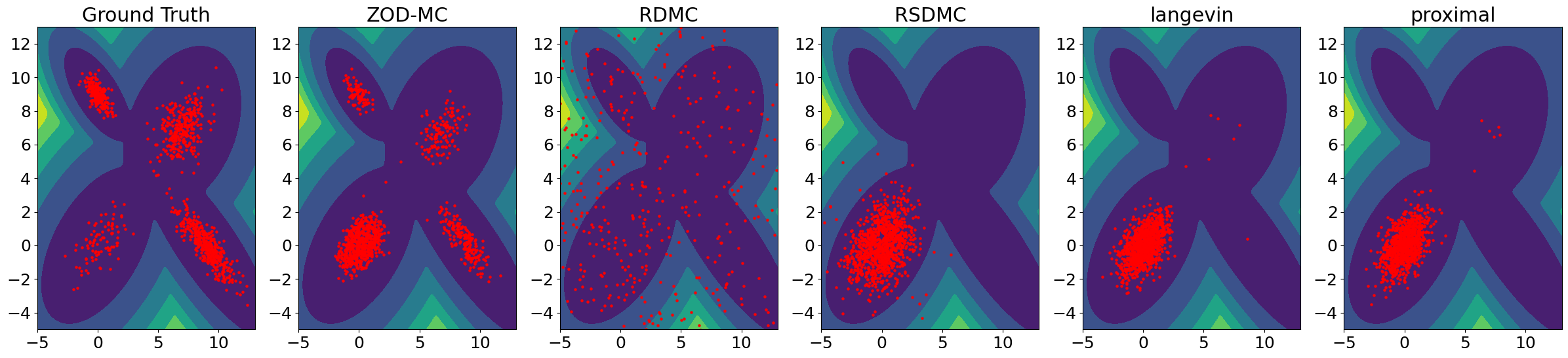
(a) Generated samples at $100$ oracle complexity per score evaluation

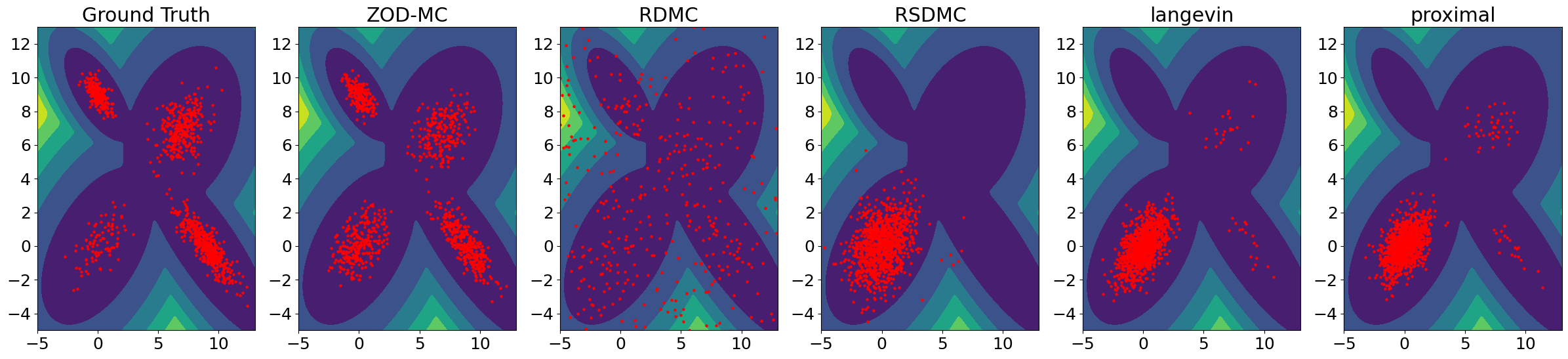
(b) Generated samples at $1100$ oracle complexity per score evaluation

(c) Generated samples at $2100$ oracle complexity per score evaluation

Figure 6: Generated Samples for GMM at different oracle complexity

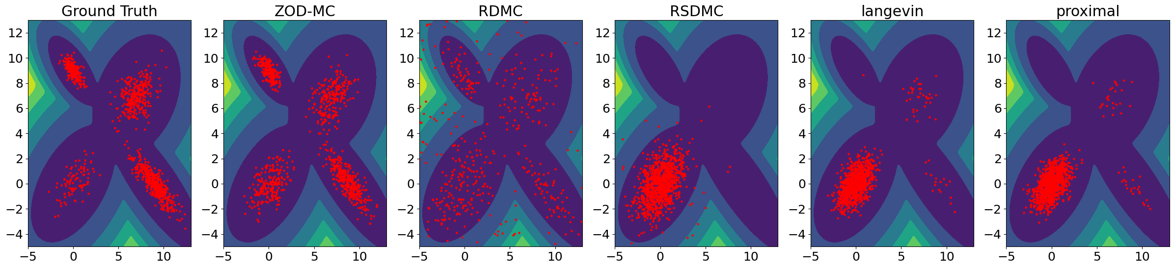
(a) Generated samples at $3100$ oracle complexity per score evaluation

(b) Generated samples at $4100$ oracle complexity per score evaluation

(c) Generated samples at $5100$ oracle complexity per score evaluation

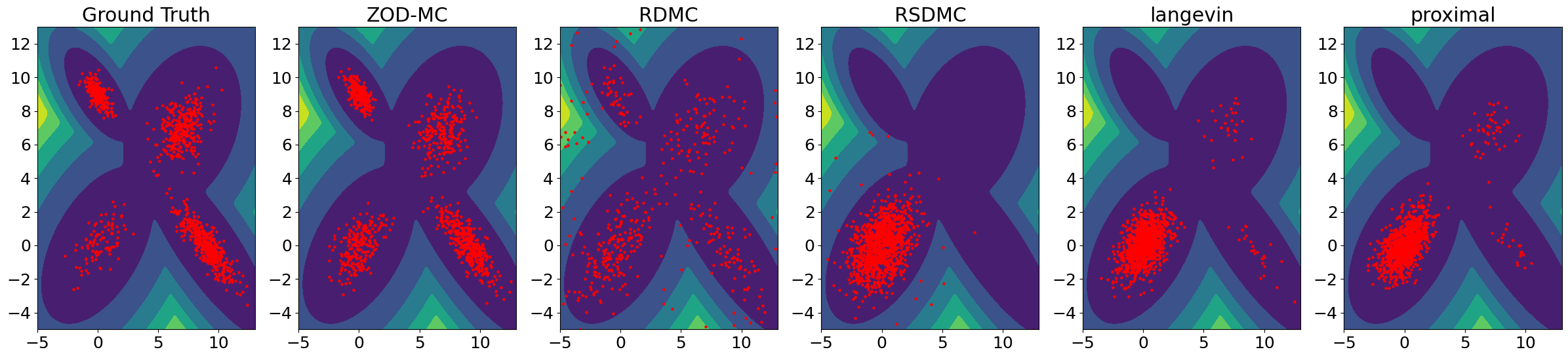
(d) Generated samples at $6100$ oracle complexity per score evaluation

Figure 7: Generated Samples for GMM at different oracle complexity

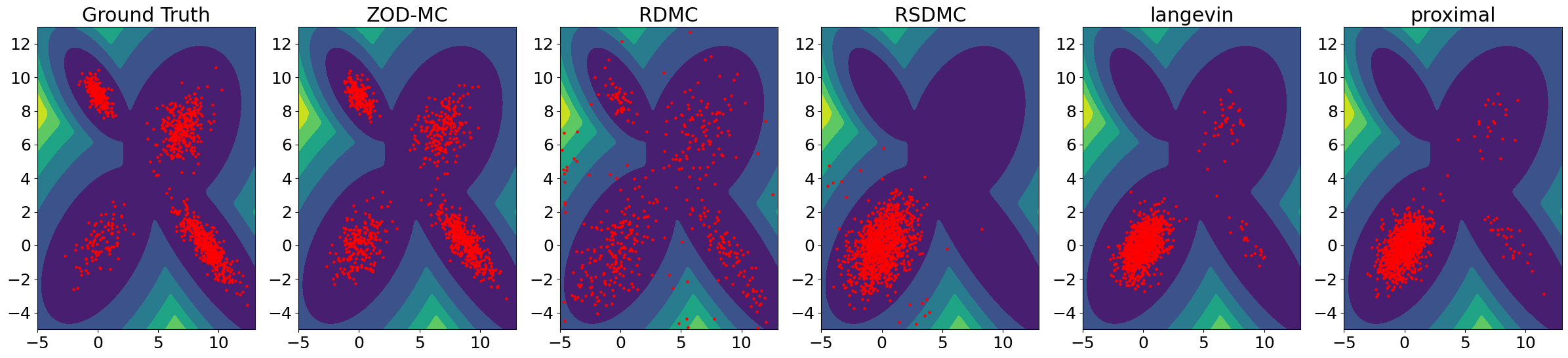
(a) Generated samples at $7100$ oracle complexity per score evaluation

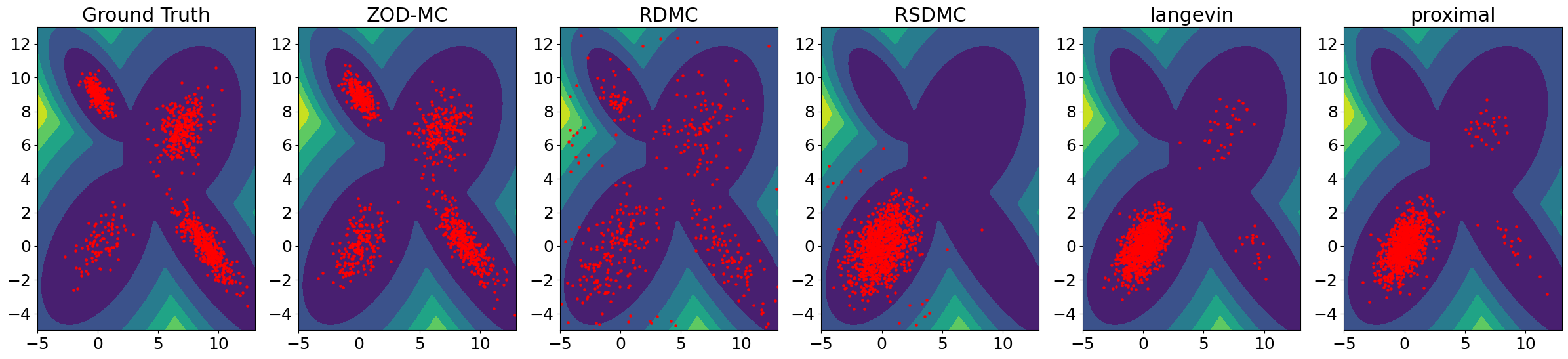
(b) Generated samples at $8100$ oracle complexity per score evaluation

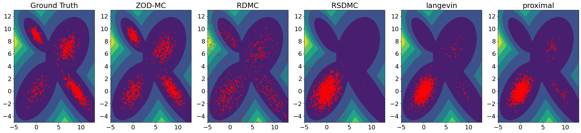
(c) Generated samples at $9100$ oracle complexity per score evaluation

Figure 8: Generated Samples for GMM at different oracle complexity

B.2 Samples from Discontinuous 2D GMM at different Oracle Complexities

We display the generated samples at different oracle complexities in Figures 9 ,10, 11. At the end we show the $W_{2}$ and MMD for this example in Figure 12.

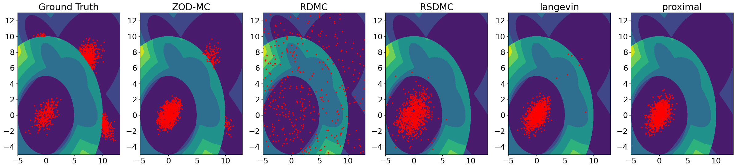
(a) Generated samples at $100$ oracle complexity per score evaluation

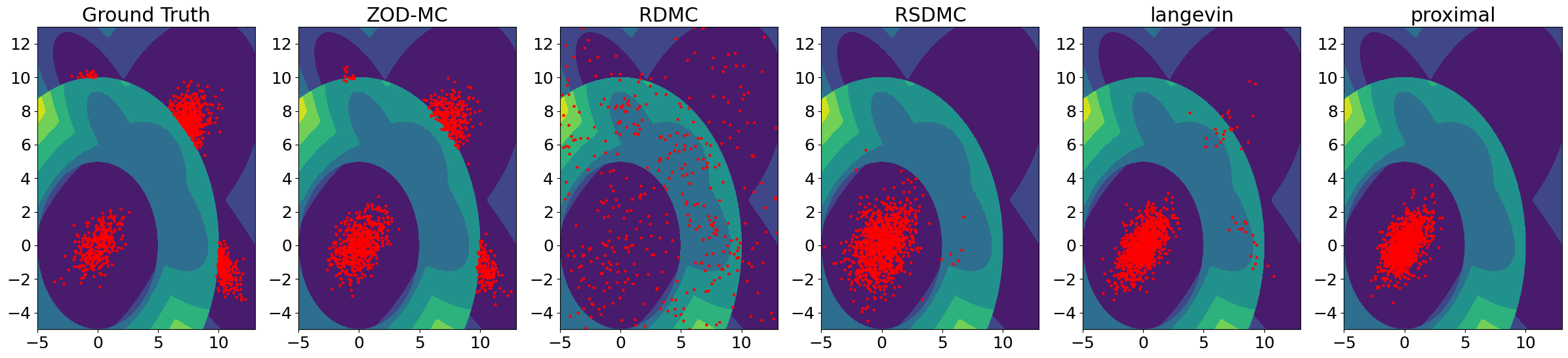
(b) Generated samples at $1100$ oracle complexity per score evaluation

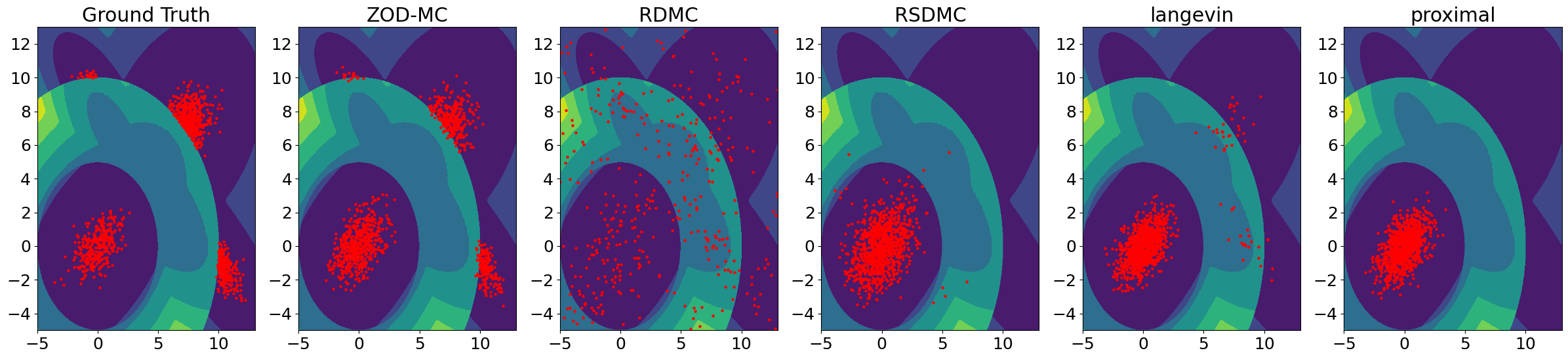
(c) Generated samples at $2100$ oracle complexity per score evaluation

Figure 9: Generated Samples for discontinuous GMM at different oracle complexity

(a) Generated samples at $3100$ oracle complexity per score evaluation

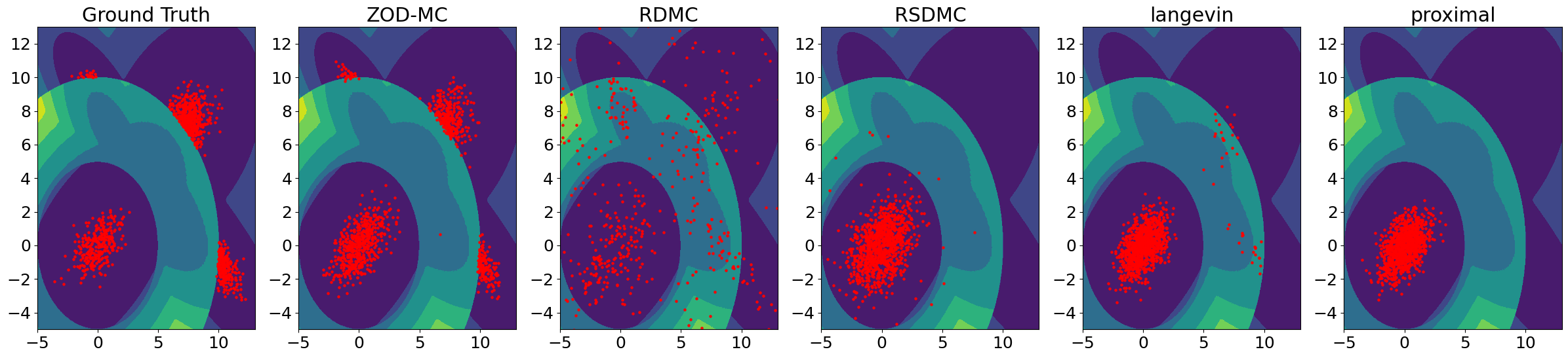
(b) Generated samples at $4100$ oracle complexity per score evaluation

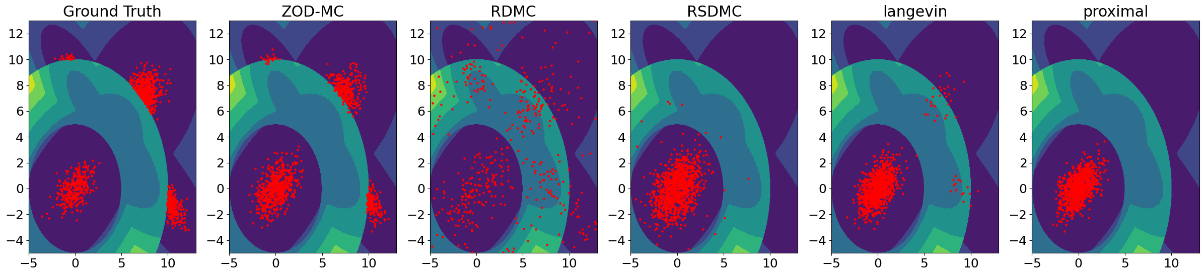
(c) Generated samples at $5100$ oracle complexity per score evaluation

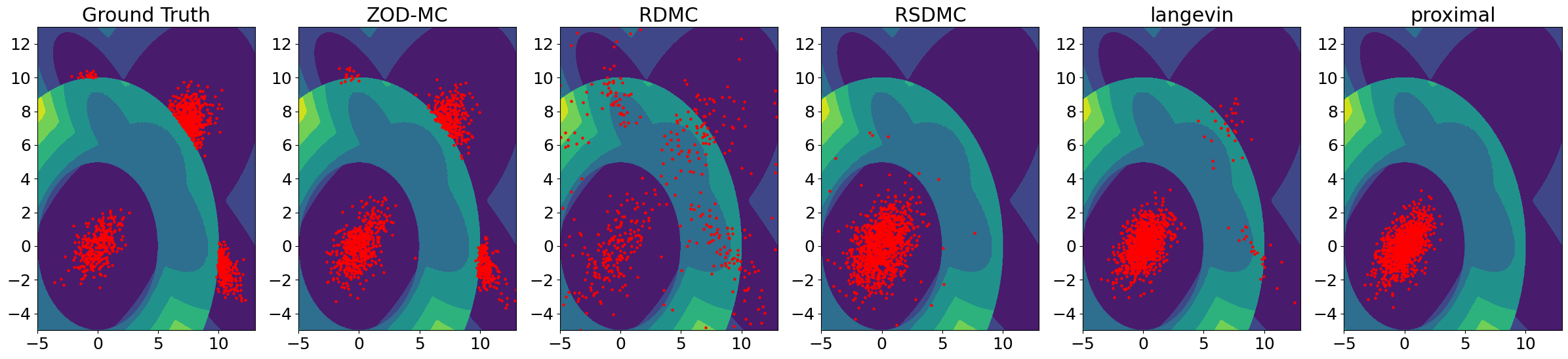
(d) Generated samples at $6100$ oracle complexity per score evaluation

Figure 10: Generated Samples for discontinuous GMM at different oracle complexity

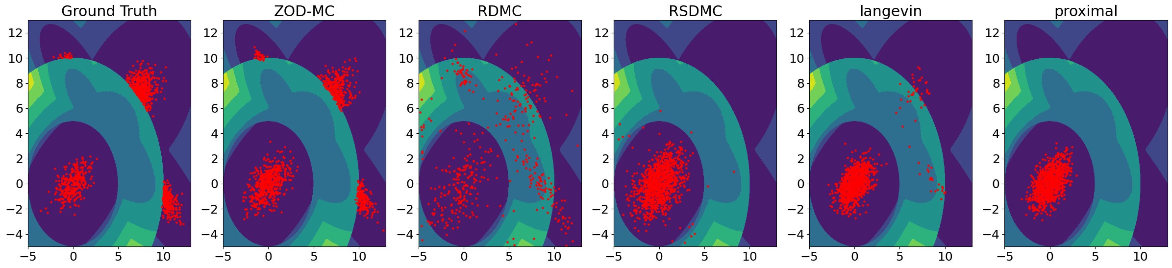
(a) Generated samples at $7100$ oracle complexity per score evaluation

(b) Generated samples at $8100$ oracle complexity per score evaluation

(c) Generated samples at $9100$ oracle complexity per score evaluation

Figure 11: Generated Samples for discontinuous GMM at different oracle complexity

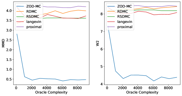
Figure 12: $W_{2}$ and MMD at different oracle complexities for discontinuous potential

B.3 Samples from different radius

We display the generated samples at different radius in Figures 13, 14.

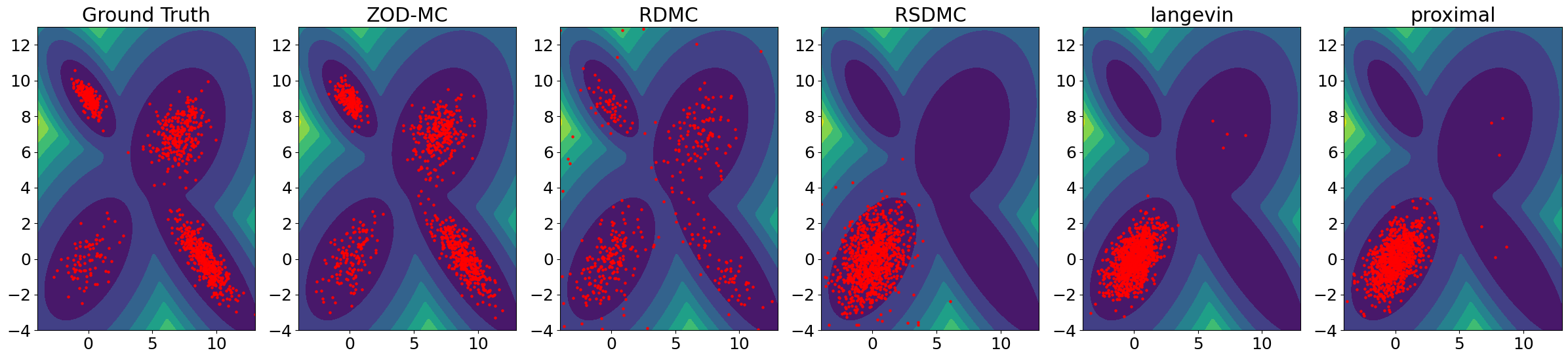
(a) Generated samples at $R=1$

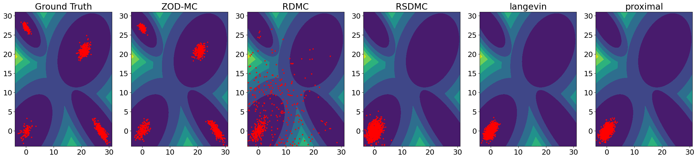
(b) Generated samples at $R=3$

Figure 13: Generated samples at different radius

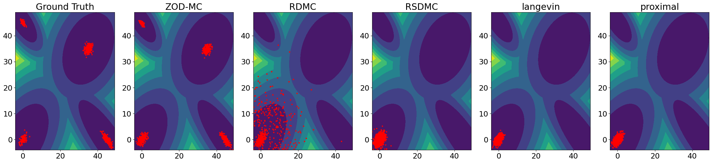
(a) Generated samples at $R=5$

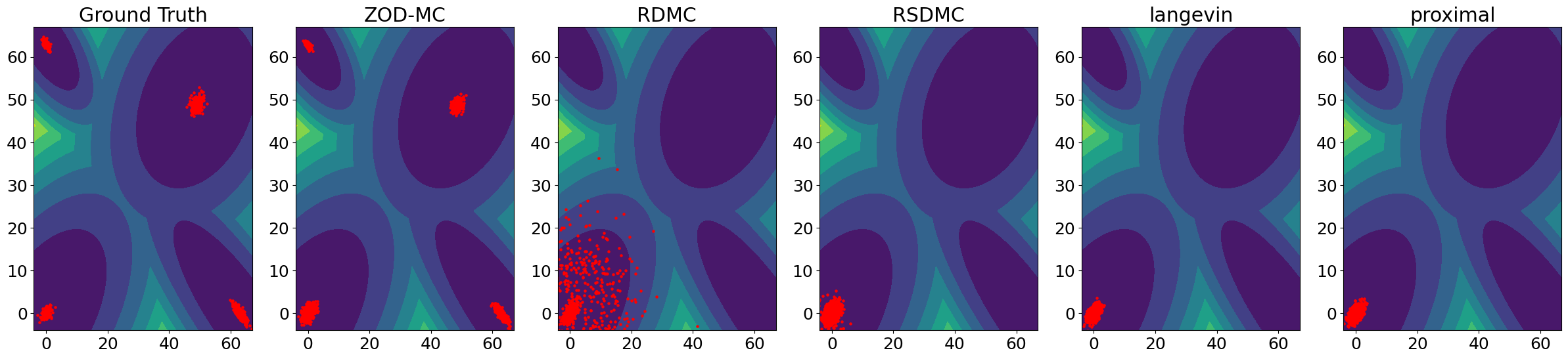
(b) Generated samples at $R=7$

(c) Generated samples at $R=9$

Figure 14: Generated samples at different radius

B.4 Muller Brown Potential Details

The potential is given by $V(x,y)=\beta\,\cdot\,(V_{m}(x,y)+V_{q}(x,y))$

$$V_{m}(x,y)=-200\exp\big{(}-(x-1)^{2}-10y^{2}\big{)}-170\exp\big{(}-6.5(x+0.5)^{2}+11(x+0.5)(y-1.5)-6.5(y-1.5)^{2}\big{)}$$

$$-100\exp\big{(}-x^{2}-10(y-0.5)^{2}\big{)}+15\exp\big{(}0.7(x+1)^{2}+0.6(x+1)(y-1)+0.7(y-1)^{2}\big{)}$$

where $V_{m}$ corresponds to the original Müller Brown and $V_{q}(x,y)=35.0136(x-x_{c}^{*})^{2}+59.8399(y-y_{c}^{*})^{2}$, with $(x_{c}^{*},y_{c}^{*})$ is approximately the minimizer at the center of the middle potential well, and $V_{q}$ is a correction introduced so that the depths of all three wells are.

References

• [1] K. Balasubramanian, S. Chewi, M. A. Erdogdu, A. Salim, and S. Zhang. Towards a theory of non-log-concave sampling: first-order stationarity guarantees for langevin monte carlo. In Conference on Learning Theory, pages 2896–2923. PMLR, 2022.
• [2] J. Benton, V. De Bortoli, A. Doucet, and G. Deligiannidis. Linear convergence bounds for diffusion models via stochastic localization. arXiv preprint arXiv:2308.03686, 2023.
• [3] H. Chen, H. Lee, and J. Lu. Improved analysis of score-based generative modeling: User-friendly bounds under minimal smoothness assumptions. In International Conference on Machine Learning, pages 4735–4763. PMLR, 2023.
• [4] S. Chen, S. Chewi, J. Li, Y. Li, A. Salim, and A. Zhang. Sampling is as easy as learning the score: theory for diffusion models with minimal data assumptions. ICLR, 2022.
• [5] Y. Chen, S. Chewi, A. Salim, and A. Wibisono. Improved analysis for a proximal algorithm for sampling. In Conference on Learning Theory, pages 2984–3014. PMLR, 2022.
• [6] Y. Chen and R. Eldan. Localization schemes: A framework for proving mixing bounds for markov chains. In 2022 IEEE 63rd Annual Symposium on Foundations of Computer Science (FOCS), pages 110–122. IEEE, 2022.
• [7] Y. Chen and K. Gatmiry. A simple proof of the mixing of metropolis-adjusted langevin algorithm under smoothness and isoperimetry. arXiv preprint arXiv:2304.04095, 2023.
• [8] S. Chewi. Log-concave sampling. 2023. Book draft available at https://chewisinho.github.io/.
• [9] S. Chewi, T. Le Gouic, C. Lu, T. Maunu, and P. Rigollet. Svgd as a kernelized wasserstein gradient flow of the chi-squared divergence. Advances in Neural Information Processing Systems, 33:2098–2109, 2020.
• [10] G. Conforti, A. Durmus, and M. G. Silveri. Score diffusion models without early stopping: finite fisher information is all you need. arXiv preprint arXiv:2308.12240, 2023.
• [11] A. S. Dalalyan and A. Karagulyan. User-friendly guarantees for the langevin monte carlo with inaccurate gradient. Stochastic Processes and their Applications, 129(12):5278–5311, 2019.
• [12] A. S. Dalalyan and L. Riou-Durand. On sampling from a log-concave density using kinetic langevin diffusions. Bernoulli, 26(3):1956–1988, 2020.
• [13] V. De Bortoli. Convergence of denoising diffusion models under the manifold hypothesis. arXiv preprint arXiv:2208.05314, 2022.
• [14] R. Dwivedi, Y. Chen, M. J. Wainwright, and B. Yu. Log-concave sampling: Metropolis-hastings algorithms are fast. Journal of Machine Learning Research, 20(183):1–42, 2019.
• [15] Y. He, K. Balasubramanian, and M. A. Erdogdu. On the ergodicity, bias and asymptotic normality of randomized midpoint sampling method. Advances in Neural Information Processing Systems, 33:7366–7376, 2020.
• [16] Y. He, K. Balasubramanian, B. K. Sriperumbudur, and J. Lu. Regularized stein variational gradient flow. arXiv preprint arXiv:2211.07861, 2022.
• [17] J. Ho, A. Jain, and P. Abbeel. Denoising diffusion probabilistic models. Advances in Neural Information Processing Systems, 33:6840–6851, 2020.
• [18] X. Huang, H. Dong, Y. Hao, Y. Ma, and T. Zhang. Monte carlo sampling without isoperimetry: A reverse diffusion approach. arXiv preprint arXiv:2307.02037, 2023.
• [19] X. Huang, D. Zou, H. Dong, Y. Ma, and T. Zhang. Faster sampling without isoperimetry via diffusion-based monte carlo. arXiv preprint arXiv:2401.06325, 2024.
• [20] H. Lee, J. Lu, and Y. Tan. Convergence of score-based generative modeling for general data distributions. In International Conference on Algorithmic Learning Theory, pages 946–985. PMLR, 2023.
• [21] Y. T. Lee, R. Shen, and K. Tian. Structured logconcave sampling with a restricted gaussian oracle. In M. Belkin and S. Kpotufe, editors, Proceedings of Thirty Fourth Conference on Learning Theory, volume 134 of Proceedings of Machine Learning Research, pages 2993–3050. PMLR, 15–19 Aug 2021.
• [22] G. Li, Y. Wei, Y. Chen, and Y. Chi. Towards faster non-asymptotic convergence for diffusion-based generative models. arXiv preprint arXiv:2306.09251, 2023.
• [23] R. Li, M. Tao, S. S. Vempala, and A. Wibisono. The mirror Langevin algorithm converges with vanishing bias. In International Conference on Algorithmic Learning Theory, pages 718–742. PMLR, 2022.
• [24] R. Li, H. Zha, and M. Tao. Sqrt(d) Dimension Dependence of Langevin Monte Carlo. In ICLR, 2021.
• [25] X. H. Li and M. Tao. Automated construction of effective potential via algorithmic implicit bias. arXiv preprint arXiv:2401.03511, 2024.
• [26] J. Liang and Y. Chen. A proximal algorithm for sampling. arXiv preprint arXiv:2202.13975, 2022.
• [27] Q. Liu. Stein variational gradient descent as gradient flow. Advances in neural information processing systems, 30, 2017.
• [28] L. Pardo. Statistical inference based on divergence measures. CRC press, 2018.
• [29] L. Richter, J. Berner, and G.-H. Liu. Improved sampling via learned diffusions. ICLR, 2024.
• [30] H. E. Robbins. An empirical bayes approach to statistics. In Breakthroughs in Statistics: Foundations and basic theory, pages 388–394. Springer, 1992.
• [31] A. Salim, L. Sun, and P. Richtarik. A convergence theory for svgd in the population limit under talagrand’s inequality t1. In International Conference on Machine Learning, pages 19139–19152. PMLR, 2022.
• [32] A. Schlichting. Poincaré and log–sobolev inequalities for mixtures. Entropy, 21(1):89, 2019.
• [33] R. Shen and Y. T. Lee. The randomized midpoint method for log-concave sampling. Advances in Neural Information Processing Systems, 32, 2019.
• [34] J. Sohl-Dickstein, E. Weiss, N. Maheswaranathan, and S. Ganguli. Deep unsupervised learning using nonequilibrium thermodynamics. ICML, 2015.
• [35] Y. Song, J. Sohl-Dickstein, D. P. Kingma, A. Kumar, S. Ermon, and B. Poole. Score-based generative modeling through stochastic differential equations. In International Conference on Learning Representations, 2021.
• [36] S. Vempala and A. Wibisono. Rapid convergence of the unadjusted langevin algorithm: Isoperimetry suffices. Advances in neural information processing systems, 32, 2019.
• [37] K. Yingxi Yang and A. Wibisono. Convergence of the inexact langevin algorithm and score-based generative models in kl divergence. arXiv e-prints, pages arXiv–2211, 2022.
• [38] Q. Zhang and Y. Chen. Path integral sampler: a stochastic control approach for sampling. ICLR, 2022.