Randomized Matrix Computations:
Themes and Variations

Abstract.

This short course offers a new perspective on randomized algorithms for matrix computations. It explores the distinct ways in which probability can be used to design algorithms for numerical linear algebra. Each design template is illustrated by its application to several computational problems. This treatment establishes conceptual foundations for randomized numerical linear algebra, and it forges links between algorithms that may initially seem unrelated.

1. Motivation

Numerical analysis and probability theory have not always been on the best interpersonal terms. Although Monte Carlo methods date back to the earliest days of numerical computation [Met87:Beginning-Monte], researchers have often been skeptical about their performance. For example, Monte Carlo algorithms for approximating integrals [QSS07:Numerical-Mathematics-2ed, Sect. 9.9.3] can only achieve low precision and their output is highly variable. This fact about this particular procedure inspired a general sentiment that randomized algorithms are unreliable tools for numerical problems:

“Our experience suggests that many practitioners of scientific computing view randomized algorithms as a desperate and final resort.”

—Halko et al. [HMT11:Finding-Structure, Rem. 1.1].

Over the last 20 years, the numerical analysis community has come to appreciate the value of probabilistic algorithms. This sea change can be attributed to the development and popularization of randomized methods that can solve large-scale problems efficiently, reliably, and robustly. In particular, the randomized SVD [HMT11:Finding-Structure, TW23:Randomized-Algorithms] has become a workhorse algorithm for obtaining low-rank matrix approximations in scientific computing and machine learning. By now, the numerical analysis literature contains a diverse collection of randomized algorithms.

This short course offers a new perspective on randomized algorithms for matrix computations. Our goal has been to identify distinct conceptual ways that probability can be used for algorithm design in numerical linear algebra. We refer to these design templates as themes. For each theme, we describe how it allows us to solve a number of basic computational problems. We refer to these examples as variations. It is our hope that this treatment highlights connections between approaches that may seem different in spirit.

1.1. The role of randomness

Common problems in numerical linear algebra include linear systems, least-squares problems, eigenvalue problems, matrix approximation, and more. Before we discuss computational approaches to these problems, we would like to clarify what we mean by a randomized algorithm and how it differs from statistical randomness.

1.1.1. Algorithmic randomness

Recall that a computer algorithm is a finite sequence of well-defined elementary steps that provably returns a solution to a well-specified computational problem. In numerical analysis, we allow approximate solutions that achieve a specified error tolerance. A randomized algorithm solves each fixed problem instance by generating random variables and using them as part of the computational procedure.

Example 1.1 (Checking matrix multiplication).

There is a simple randomized algorithm for testing whether we have correctly multiplied two matrices. Given square $n\times n$ matrices $(\bm{A},\bm{B},\bm{C})$ with integer entries, we would like to confirm whether $\bm{C}=\bm{AB}$ without performing a matrix multiplication. An inexpensive algorithm is to draw a random vector $\bm{x}\sim\textsc{uniform}\{\pm 1\}^{n}$ and form the matrix–vector products $\bm{C}\bm{x}$ and $\bm{A}(\bm{B}\bm{x})$. If the two vectors are unequal, then we can confidently report false. If the two vectors are equal, then we report true even though it is possible that our judgment is wrong.

Since this procedure can fail with nonzero probability, it is called a Monte Carlo-style randomized algorithm. Most of the algorithms we discuss are Monte Carlo-style methods where the outcome is random. Fortunately, it is often inexpensive to check whether they have returned the correct answer.

Example 1.2 (Maximum eigenvalue).

The randomized power method is a familiar algorithm for approximating the maximum eigenvalue of a positive-semidefinite matrix $\bm{A}$ to a specified relative error. It begins with a random vector $\bm{x}\sim\textsc{normal}(\bm{0},\mathbf{I})$ and repeatedly applies the matrix to the vector to obtain a sequence of maximum eigenvalue estimates:

$$\xi_{t}=\bm{x}^{*}(\bm{A}^{t}\bm{x})/\bm{x}^{*}\bm{x}\quad\text{for $t=0,1,2,3,\dots$.}$$

After a sufficient number of steps, we hope that the estimate $\xi_{t}$ approximates the maximum eigenvalue within a specified relative error tolerance. We will see that this approach succeeds with probability one. See Section 3.1 for more details about the randomized power method.

Although this method eventually succeeds, its runtime is a random variable. A procedure with a random runtime is called a Las Vegas-style randomized algorithm. We will encounter several more algorithms of this type.

1.1.2. Statistical randomness

In sharp contrast, statistical randomness is the idea of using probability to model a computational problem or to describe the behavior of an algorithm. Aside from a short overview here, this course does not consider the role of statistical randomness in numerical analysis.

Statisticians often model observations as independent samples from an underlying population. This perspective leads to the concept of average-case analysis, where we ask how an algorithm performs for a problem instance drawn at random from some distribution. For examples in numerical linear algebra, see Demmel’s paper [Dem88:Probability-Numerical].

In many scientific fields, data collection involves both measurement errors and uncertainty. To address these issues, numerical analysts study the sensitivity of mathematical problem formulations to perturbations of the data. They also study the stability of algorithms under changes in the input. Historically, these analyses dealt with the worst choice of perturbation of a given magnitude. See [Hig02:Accuracy-Stability] for discussion.

As another application of statistical randomness to numerical analysis, we can model perturbations of problem data using probability. We can try to understand how much the answer to a computational problem is likely to change under a random perturbation. We can also try to assess how a random perturbation of the problem data impacts the performance of a particular algorithm, which is called a smoothed analysis of the algorithm [ST02:Smoothed-Analysis]. We will see that smoothed analysis has computational implications for linear algebra (LABEL:sec:smoothed-analysis).

Numerical analysts have also worked hard to understand the effects of rounding errors on the output of numerical algorithms. The worst-case analysis is quite pessimistic, which motivates us to consider statistical models for rounding errors. This idea was already considered in 1951 by Goldstine & von Neumann [GvN51:Numerical-Inverting-II] in their work on solving linear systems. Higham and coauthors have recently revisited the probabilistic analysis of rounding errors [HM19:New-Approach, CH23:Probabilistic-Rounding]. Computationally, we can also exploit the beneficial effects of random rounding errors by using stochastic rounding procedures [CHM21:Stochastic-Rounding].

Analysis based on statistical randomness has been a useful paradigm for understanding numerical computation. Nevertheless, statistical randomness imposes the modeling assumption that the problem data, perturbations to the problem data, or errors made during computations can be treated as random quantities. By contrast, algorithmic randomness is injected into the computational procedure in a controlled manner by the algorithm designer, allowing for numerical methods that are provably effective for arbitrary inputs.

1.1.3. Statistical behavior of randomized algorithms

Keep in mind that randomized algorithms for matrix computations produce statistical output. Therefore, we can use tools from statistical theory to understand the distribution of the output or even to develop more effective algorithms.

Example 1.3 (Majority vote).

Consider a randomized algorithm for a decision problem that gives the correct result with probability $p>0.5$. Although we may not have a lot of confidence in the output from a single run of the algorithm, we can run the algorithm $n$ times and take a majority vote. (Were the trials more often true or false?) To obtain failure probability $\delta\in(0,1)$, it is sufficient to perform $n\geq(p-0.5)^{-2}\log(1/\delta)$ independent repetitions. This approach can dramatically increase the reliability of the basic algorithm.

Statistical theory can also be used to equip the output of a randomized algorithm with a confidence interval; see Section 2.1.6 for an application to the problem of trace estimation. We can also use insights from the design of statistical estimators to develop better algorithms, e.g., whose output is less variable; see Section 2.1.7 for some discussion.

We will not emphasize the nexus between statistics and computation, but this link offers potential opportunities for supercharging the methods that we discuss.

1.2. Prerequisites

This course is intended for advanced undergraduates, beginning graduate students, and curious researchers in the mathematical sciences. On the mathematical side, we assume a thorough knowledge of linear algebra, matrix analysis, applied probability, and basic statistics. On the computational side, you should understand the basic principles of computer algorithms, and we expect that you have taken a first course on numerical linear algebra. If you have followed everything in the introduction so far, you’re probably in good shape.

1.3. Other resources

As a classical reference on matrix computations, the book of Golub & Van Loan [GVL13:Matrix-Computations-4ed] is a comprehensive and trusted source.

The second author has written several surveys and sets of lecture notes on aspects of randomized matrix computations. These resources are available from the website https://tropp.caltech.edu/. The current notes borrow heavily from this body of work.

• Finding structure with randomness [HMT11:Finding-Structure]. This survey provides a framework for randomized SVD algorithms for low-rank matrix approximation. The paper includes pseudocode for reliable algorithms, a number of applications in scientific computing and machine learning, and the first theoretical analysis that can predict the detailed behavior of these algorithms.

• An introduction to matrix concentration inequalities [Tro15:Introduction-Matrix]. This monograph provides a comprehensive introduction to matrix concentration inequalities, which are basic tools for studying random matrices. It explains how these results can be used to analyze probabilistic methods for matrix computation, including matrix Monte Carlo methods and randomized dimension reduction schemes. These notes support a tutorial given at NeurIPS 2012.

• Matrix concentration and computational linear algebra [Tro19:Matrix-Concentration-LN]. These notes accompany a short course taught at École Normale Supérieure in Paris in July 2019. They present some foundational results on matrix concentration for independent sums and martingales, and they include detailed applications to quantum state tomography, sparsification of graphs, and the analysis of the near-linear-time graph Laplacian solver of Kyng & Sachdeva [KS16:Approximate-Gaussian].

• Randomized algorithms for matrix computations [Tro20:Randomized-Algorithms-LN]. These notes were written to support a quarter class on randomized matrix computations taught at Caltech in the Winter 2020 term. The material includes trace estimation, eigenvalue computations, low-rank matrix approximation, matrix concentration, matrix Monte Carlo methods, randomized dimension reduction, and more.

• Randomized numerical linear algebra [MT20:Randomized-Numerical]. This survey was invited to the 2020 volume of Acta Numerica. It covers a significant proportion of the literature on randomized matrix computations, with a focus on methods that are reliable in practice.

• Randomized algorithms for low-rank matrix approximation [TW23:Randomized-Algorithms]. This survey updates the randomized SVD paper [HMT11:Finding-Structure] to include more modern approaches based on Krylov subspace methods. It also treats Nyström approximations of psd matrices. In addition, the paper showcases scientific applications in genetics and in molecular biophysics.

  There are several other treatises on randomized matrix computations. For a theoretical computer science perspective, see the notes [Woo14:Sketching-Tool, KV17:Randomized-Algorithms, DM18:Lectures-Randomized]. The monograph [MDM+23:Randomized-Numerical] discusses the RandBLAS primitives and the RandLAPack library that are currently under development.

  1.4. Notation

  We employ standard notation that, hopefully, is self-explanatory. In most places, the initial appearance of a symbol is accompanied by a reminder about what it means. If you want to gird yourself first, this section will acquaint you with the main pieces of notation.

  We work primarily in the real field $\mathbb{R}$, although large parts of the discussion extend to matrices with entries in the complex field $\mathbb{C}$. All logarithms have the natural base $\mathrm{e}$. The Pascal notation $\coloneqq$ or $\eqqcolon$ generates a definition.

  We use lowercase italic letters ($a,b,c$) for scalar variables. Lowercase bold italic letters ($\bm{a},\bm{b},\bm{c}$) refer to vectors, which are always column vectors. Uppercase bold italic letters ($\bm{A},\bm{B},\bm{C}$) denote matrix variables. The symbol $\mathbf{e}_{j}$ is the $j$th standard basis vector. The letter $\mathbf{I}$ or $\mathbf{I}_{n}$ represents a square identity matrix; the subscript specifies the dimension. The symbol ${}^{*}$ is the (conjugate) transpose of a vector or matrix. The dagger ${}^{\dagger}$ refers to the Moore–Penrose pseudoinverse of a matrix.

  We equip the Euclidean space $\mathbb{R}^{n}$ with the standard inner product $\langle{\cdot},\ {\cdot}\rangle$ and the norm $\|{\cdot}\|_{2}$. There are several ways to express the coordinates of a vector or a matrix. To denote the $(j,k)$ entry of a matrix $\bm{A}$, we may write $a_{jk}$ or use the functional notation $\bm{A}(j,k)$. The symbol $\bm{A}(i,:)$ refers to the $i$th row of the matrix, while $\bm{A}(:,j)$ refers to the $j$th row of the matrix. As a warning, $\bm{a}_{k}$ may refer to either the $k$th row or the $k$th column of the matrix, depending on context. In some settings, we must extract components with respect to bases other than the standard basis.

  The linear space $\mathbb{M}_{n}(\mathbb{R})$ comprises all square $n\times n$ matrices. The real-linear subspace $\mathbb{H}_{n}(\mathbb{R})$ comprises the real, symmetric matrices with dimension $n$. Each of these matrices has $n$ real eigenvalues, arranged in decreasing order: $\lambda_{1}\geq\lambda_{2}\geq\dots\geq\lambda_{n}$. The cone $\mathbb{H}_{n}^{+}(\mathbb{R})$ contains the positive-semidefinite (psd) matrices, those symmetric matrices whose eigenvalues are all nonnegative. For a pair $(\bm{A},\bm{B})$ of symmetric matrices, the semidefinite relation $\bm{A}\preccurlyeq\bm{B}$ means that $\bm{B}-\bm{A}$ is a psd matrix.

  For a general matrix $\bm{B}\in\mathbb{R}^{m\times n}$, we list the singular values in decreasing order:

  $$\sigma_{\max}\coloneqq\sigma_{1}\geq\sigma_{2}\geq\dots\geq\sigma_{n}\eqqcolon\sigma_{\min}.$$

  The spectral condition number is the matrix function $\kappa\coloneqq\sigma_{\max}/\sigma_{\min}$. We frequently use the Frobenius norm $\|{\cdot}\|_{\mathrm{F}}$, the spectral norm $\|{\cdot}\|$, and the trace norm $\|{\cdot}\|_{*}$.

  Everything takes place in an (unspecified) probability space that is big enough to support all of the random variables we consider. We often use letters at the end of the alphabet to refer to random variables, while maintaining our other conventions. For instance, $X$ is a scalar random variable, $\bm{x}$ is a vector-valued random variable, and $\bm{X}$ is a random matrix. The symbol $\sim$ means “has the distribution”. Small capitals are reserved for named distributions (normal, uniform). The abbreviation “i.i.d.” means independent and identically distributed. Random variables with hats, such as $\widehat{\bm{x}}$, generally refer to estimators.

  The symbol $\mathbb{P}$ reports the probability of an event. The operator $\operatorname{\mathbb{E}}$ returns the expectation of a random variable, computed entrywise for vectors or matrices. We use subscripts to denote partial expectations, so $\operatorname{\mathbb{E}}_{X}$ is the expectation with respect to the randomness in $X$. The partial expectation is only used when there is no possibility for confusion (e.g., $X$ is independent from everything else).

  We use the computer science interpretation of the $\mathcal{O}$ symbol. For example, $\mathcal{O}(n)$ is the class of functions that grow no more quickly than $n$ as $n\to\infty$.

  2. Monte Carlo approximation

  Already in the earliest days of numerical computation, scientists were exploring randomized algorithms for approximating complicated physical models [Met87:Beginning-Monte]. Enrico Fermi is credited with using statistical sampling methods to simulate neutron diffusion in the 1930s. Instead of tracking the full dynamical process, he randomly constructed the next segment of an individual neutron trajectory. The computations were often performed with a mechanical adding machine. Independently, in 1946 and 1947, Stanislaw Ulam and John von Neumann proposed a similar model for neutron diffusion as a trial problem for the newly constructed ENIAC computer. In late 1947, Nick Metropolis and Klari von Neumann designed an implementation, and they performed the first tests of the Monte Carlo method on the ENIAC.

  Today, every student of numerical analysis learns about Monte Carlo methods as a technique for approximating a complicated integral, especially of a high-dimensional function [QSS07:Numerical-Mathematics-2ed, Sect. 9.9.3]. In this application, we draw a random variable that has the same distribution as the integrand. To reduce the variance of this simple estimator, we can draw independent samples and average them together.

  Although Monte Carlo methods are an ancient part of numerical analysis, their advent in numerical linear algebra is more recent.

  Theme (Monte Carlo approximation).

  Construct a simple unbiased estimator of a complicated linear-algebraic quantity. Reduce the variance by averaging independent copies of the estimator.

  This section describes how Monte Carlo approximation can be applied to two problems in matrix computations. In Section 2.1, we consider how to estimate a specific scalar quantity, the trace of a square matrix. In Section 2.2, we explain how related ideas allow us to estimate a matrix quantity, such as the product of two matrices. We also provide citations to papers that formulate other applications of Monte Carlo approximation in numerical linear algebra.

  2.1. Trace estimation

  Let us begin with an approachable example of scalar Monte Carlo approximation in linear algebra. The goal is to estimate the trace of a square matrix using as few matrix–vector products as possible. We will introduce a randomized algorithm for this task and describe some elements of the analysis. This approach, due to Girard [Gir89:Fast-Monte-Carlo], stands among the oldest examples of probability in matrix computations. Our treatment follows [MT20:Randomized-Numerical, Tro20:Randomized-Algorithms-LN].

  2.1.1. Implicit trace estimation

  Suppose that we are given a square matrix $\bm{A}\in\mathbb{M}_{n}(\mathbb{R})$. Our goal is to compute the trace:

  $$\operatorname{tr}(\bm{A})\coloneqq\sum_{i=1}^{n}a_{ii}.$$

  Of course, the problem is trivial if we can access the diagonal entries of $\bm{A}$ at low computational cost. In this case, revealing and summing the diagonal entries takes about $\mathcal{O}(n)$ arithmetic operations.

  Instead, assume that we have access to the matrix via matrix–vector products (matvecs). That is, given a vector $\bm{x}\in\mathbb{R}^{n}$, we can form the product $\bm{x}\mapsto\bm{A}\bm{x}$ at a reasonable cost. We will justify this model in Section 2.1.2. For now, our task is to determine $\operatorname{tr}(\bm{A})$ using as few matvecs as possible.

  As before, we can complete this job by using matvecs to read off the diagonal entries of the matrix:

  $$a_{ii}=\mathbf{e}_{i}^{*}(\bm{A}\mathbf{e}_{i})\quad\text{for each $i=1,2,3,\dots,n$.}$$

  The symbol $\mathbf{e}_{i}$ denotes the $i$th standard basis vector in $\mathbb{R}^{n}$. This procedure provides an exact value for the trace, but it requires fully $n$ matvec operations. The cost may be prohibitive when $n$ is large.

  Fortunately, in many settings, it is acceptable to produce an approximation for the trace if we can reduce the number of matvecs substantially.

  Problem (Implicit trace estimation).

  Suppose that $\bm{A}$ is a square matrix, accessible via matvecs: $\bm{x}\mapsto\bm{A}\bm{x}$. The task is to approximate $\operatorname{tr}(\bm{A})$ while limiting the number of matvecs.

  2.1.2. Applications of trace estimation

  Although the implicit trace estimation problem may seem unnatural, it arises in a wide range of applications. These domains include statistical computation, network science, chemical graph theory, and quantum statistical mechanics.

  • Smoothing splines [Gir89:Fast-Monte-Carlo, Hut90:Stochastic-Estimator]. When fitting a smoothing spline to scattered data, we need to estimate $\operatorname{tr}(\bm{A}^{-1})$, the trace of a matrix inverse, to perform generalized cross-validation for the smoothing parameter. In this context, the matrix $\bm{A}$ is a tridiagonal matrix that models a second-difference operator. We can apply the inverse to a vector in $\mathcal{O}(n)$ arithmetic operations using a Cholesky factorization and triangular substitution.

  • Social network analysis [al2018triangle]. We can count triangles in a graph to measure the centrality of nodes in a social network. This task reduces to computing $\operatorname{tr}(\bm{A}^{3})$, where $\bm{A}$ is the adjacency matrix of the graph. We can apply the third power $\bm{A}^{3}$ to a vector by repeated multiplication.

  • Chemical graph theory [estrada2022many]. The folding degree of long-chain proteins can be measured using the Estrada index, which is defined as $\operatorname{tr}(\mathrm{e}^{\bm{A}})$. In this setting, $\bm{A}$ is a tridiagonal matrix whose diagonal is related to the dihedral angles between planes in the folded protein.

  • Quantum statistical mechanics [CH23:Krylov-Aware, ETW24:XTrace]. We can use trace estimation to compute the partition function $\operatorname{tr}(\mathrm{e}^{-\beta\bm{H}})$ and the (unnormalized) average energy $\operatorname{tr}(\bm{H}\mathrm{e}^{-\beta\bm{H}})$ of a quantum mechanical system described by a Hamiltonian matrix $\bm{H}$. We can approximate these exponentials efficiently using low-degree polynomials or Krylov subspace methods.

    See the survey [US17:Applications-Trace] for further discussion and examples.

    2.1.3. The role of randomness

    In 1989, Girard [Gir89:Fast-Monte-Carlo] proposed an elegant Monte Carlo approximation algorithm for the implicit trace estimation problem. Hutchinson [Hut90:Stochastic-Estimator] described a variant of Girard’s method that has become popular. Both of these authors were concerned with cross-validation for smoothing splines. Here is the idea.

    Suppose that $\bm{x}\in\mathbb{R}^{n}$ is a random test vector whose distribution is isotropic:

    $$\operatorname{\mathbb{E}}[\bm{xx}^{*}]=\mathbf{I}_{n}.$$

    Many familiar distributions are isotropic:

    • Standard normal. A random vector $\bm{x}\sim\textsc{normal}(\bm{0},\mathbf{I}_{n})$ with independent standard normal entries is isotropic.

    • Uniform on a sphere. A random vector $\bm{x}\sim\textsc{uniform}(\sqrt{n}\mathbb{S}^{n-1})$ distributed uniformly on the Euclidean sphere with radius $\sqrt{n}$ is isotropic.

    • Independent signs. A random vector $\bm{x}\sim\textsc{uniform}\{\pm 1\}^{n}$ whose entries are independent and take values $\pm 1$ with equal probability is isotropic.

      These distributions all have a lot of randomness, which helps us build estimators with low variance.

      Let $\bm{A}\in\mathbb{M}_{n}(\mathbb{R})$ be a square input matrix. Taking one matvec with the matrix $\bm{A}$, we can form the scalar random variable

      $$Y\coloneqq\bm{x}^{*}(\bm{A}\bm{x}).$$

      Observe that $Y$ is an unbiased estimator for the trace of the matrix:

      $$\operatorname{\mathbb{E}}[Y]=\operatorname{\mathbb{E}}[\operatorname{tr}(\bm{x}^{*}\bm{A}\bm{x})]=\operatorname{\mathbb{E}}[\operatorname{tr}(\bm{A}\bm{xx}^{*})]=\operatorname{tr}(\bm{A}\cdot\operatorname{\mathbb{E}}[\bm{xx}^{*}])=\operatorname{tr}(\bm{A}).$$

      We have used the cyclic property of the trace, the linearity of the trace and the expectation, and the assumption that the test vector $\bm{x}$ has an isotropic distribution.

      Although the simple trace estimator $Y$ is correct on average, its fluctuations may be large in comparison with $\operatorname{tr}(\bm{A})$. A standard remedy is to average independent copies of the simple trace estimator. Taking $s$ matvecs with the matrix $\bm{A}$, we can form the Monte Carlo trace estimator:

      $$\widehat{\operatorname{tr}}_{s}\coloneqq\frac{1}{s}\sum_{i=1}^{s}Y_{i}\quad\text{where $Y_{i}\sim Y$ i.i.d.}$$

      By linearity, the trace estimator $\widehat{\operatorname{tr}}_{s}$ remains unbiased. By independence of the summands, we have reduced the variance by a factor of $s$ over the simple estimator. Altogether,

      $$\operatorname{\mathbb{E}}[\widehat{\operatorname{tr}}_{s}]=\operatorname{tr}(\bm{A})\quad\text{and}\quad\operatorname{Var}[\widehat{\operatorname{tr}}_{s}]=\frac{1}{s}\operatorname{Var}[Y].$$ (2.1)

      Of course, we still need to control $\operatorname{Var}[Y]$, the variance of the simple estimator, to confirm that the trace estimator $\widehat{\operatorname{tr}}_{s}$ is precise enough to employ in practice. Algorithm 1 presents pseudocode for the basic method.

      1Input matrix $\bm{A}\in\mathbb{M}_{n}(\mathbb{R})$, number $s$ of samples

      2Trace estimate $\widehat{\operatorname{tr}}_{s}$, an estimate $\widehat{v}_{s}$ for the variance of $\widehat{\operatorname{tr}}_{s}$  

      3function TraceEstimate($\bm{A}$, $s$)

      4     for $i=1,\dots,s$ do

      5         Sample isotropic random vector $\bm{x}_{i}\in\mathbb{R}^{n}$ $\triangleright$ For example, $\bm{x}_{i}\sim\textsc{uniform}\{\pm 1\}^{n}$

      6         $Y_{i}={\bm{x}_{i}}^{*}(\bm{A}\bm{x}_{i})$ $\triangleright$ One matvec      

      7     $\widehat{\operatorname{tr}}_{s}=s^{-1}\sum_{i=1}^{s}Y_{i}$ $\triangleright$ Trace estimator

      8     $\widehat{v}_{s}=(s(s-1))^{-1}\sum_{i=1}^{s}(Y_{i}-\widehat{\operatorname{tr}}_{s})^{2}$ $\triangleright$ Variance estimate for trace estimator

      Algorithm 1 Trace estimation: Simplest Monte Carlo method.

      2.1.4. Trace estimation: A priori bounds

      It remains to assess how many samples $s$ are sufficient for the Monte Carlo estimator $\widehat{\operatorname{tr}}_{s}$ to approximate $\operatorname{tr}(\bm{A})$ within a specified tolerance. This analysis hinges on the variance of the simple trace estimator.

      For ease of exposition, assume that the input matrix $\bm{A}\in\mathbb{H}_{n}^{+}(\mathbb{R})$ is a real symmetric positive-semidefinite (psd) matrix that is not zero. We also assume that the test vector follows the independent sign distribution: $\bm{x}\sim\textsc{uniform}\{\pm 1\}^{n}$.

      With these assumptions, the simple trace estimator $Y=\bm{x}^{*}(\bm{A}\bm{x})$ remains unbiased: $\operatorname{\mathbb{E}}[Y]=\operatorname{tr}(\bm{A})$. We can also obtain an exact expression for the variance:

      $$\operatorname{Var}[Y]=2\sum_{i\neq j}a_{ij}^{2}\leq 2\|{\bm{A}}\|_{\mathrm{F}}^{2}.$$

      Here and elsewhere, $\|{\cdot}\|_{\mathrm{F}}$ is the Frobenius norm. Since $\bm{A}$ is psd, its eigenvalues $\lambda_{1},\dots,\lambda_{n}$ are nonnegative. Therefore, we have the upper bound

      $$\operatorname{Var}[Y]=2\|{\bm{A}}\|_{\mathrm{F}}^{2}=2\sum_{i=1}^{n}\lambda_{i}^{2}\leq 2\big{(}\max\nolimits_{j=1,\dots,n}\lambda_{j}\big{)}\sum_{i=1}^{n}\lambda_{i}=2\|{\bm{A}}\|\operatorname{tr}(\bm{A}).$$

      As usual, $\|{\cdot}\|$ is the spectral norm. This inequality compares the variance of the estimator with the trace that we are trying to estimate.

      The variance is a quadratic functional, so we would like to place it on the scale of the squared trace. This step yields the bound

      $$\frac{\operatorname{Var}[Y]}{\operatorname{tr}(\bm{A})^{2}}\leq\frac{2\|{\bm{A}}\|}{\operatorname{tr}(\bm{A})}.$$

      To interpret this result, let us make a definition.

      Definition 2.1 (Intrinsic dimension).

      For a nonzero psd matrix $\bm{A}\in\mathbb{H}_{n}^{+}(\mathbb{R})$, the intrinsic dimension is the quantity

      $$\operatorname*{int\,dim}(\bm{A})\coloneqq\frac{\operatorname{tr}(\bm{A})}{\|{\bm{A}}\|}.$$

      We define $\operatorname*{int\,dim}(\bm{0})\coloneqq 0$.

      If $\bm{A}\in\mathbb{H}_{n}^{+}(\mathbb{R})$ is nonzero, then $1\leq\operatorname*{int\,dim}(\bm{A})\leq n$. The lower bound is attained if and only if $\bm{A}$ has rank one. The upper bound is attained if and only if $\bm{A}$ is a scalar matrix: $\bm{A}=\alpha\mathbf{I}_{n}$ for $\alpha>0$. More generally, we think about the intrinsic dimension as a continuous proxy for the rank of the matrix.

      It follows that the variance of the simple trace estimator $Y$ is inversely proportional to the intrinsic dimension of the target matrix:

      $$\frac{\operatorname{Var}[Y]}{\operatorname{tr}(\bm{A})^{2}}\leq\frac{2}{\operatorname*{int\,dim}(\bm{A})}.$$

      As a consequence of (2.1), the Monte Carlo estimator $\widehat{\operatorname{tr}}_{s}$ with $s$ independent sign vectors satisfies the variance bound

      $$\frac{\operatorname{Var}[\widehat{\operatorname{tr}}_{s}]}{\operatorname{tr}(\bm{A})^{2}}\leq\frac{2}{s\cdot\operatorname*{int\,dim}(\bm{A})}.$$ (2.2)

      Let us emphasize that this calculation depends on the distribution of the test vector $\bm{x}$. We arrive at the following statement.

      Proposition 2.2 (Monte Carlo trace estimation).

      Assume that $\bm{A}\in\mathbb{H}_{n}^{+}(\mathbb{R})$ is a nonzero psd matrix. Form the Monte Carlo trace estimator $\widehat{\operatorname{tr}}_{s}$ with $s$ independent sign vectors:

      $$\widehat{\operatorname{tr}}_{s}\coloneqq\frac{1}{s}\sum_{i=1}^{s}\bm{x}_{i}^{*}(\bm{A}\bm{x}_{i})\quad\text{where $\bm{x}_{i}\sim{\textup{{uniform}}}\{\pm 1\}^{n}$ i.i.d.}$$

      For any tolerance $\varepsilon>0$, the estimator satisfies the probability bound

      $$\mathbb{P}\left\{|{\widehat{\operatorname{tr}}_{s}-\operatorname{tr}(\bm{A})}|\geq\varepsilon\operatorname{tr}(\bm{A})\right\}\leq\frac{2}{\varepsilon^{2}s\cdot\operatorname*{int\,dim}(\bm{A})}.$$ (2.3)

      In particular, the probability bound is nontrivial as soon as the number $s$ of samples satisfies

      $$s\geq 2\varepsilon^{-2}(\operatorname*{int\,dim}(\bm{A}))^{-1}.$$ (2.4)

      Proof.

      This result follows from an easy application of Chebyshev’s inequality:

      $$\mathbb{P}\left\{|{\widehat{\operatorname{tr}}_{s}-\operatorname{tr}(\bm{A})}|\geq\varepsilon\operatorname{tr}(\bm{A})\right\}\leq\frac{\operatorname{\mathbb{E}}|{\widehat{\operatorname{tr}}_{s}-\operatorname{tr}(\bm{A})}|^{2}}{\varepsilon^{2}\cdot\operatorname{tr}(\bm{A})^{2}}=\frac{\operatorname{Var}[\widehat{\operatorname{tr}}_{s}]}{\varepsilon^{2}\cdot\operatorname{tr}(\bm{A})^{2}}\leq\frac{2}{\varepsilon^{2}s\cdot\operatorname*{int\,dim}(\bm{A})}.$$

      The equality holds because $\operatorname{\mathbb{E}}[\widehat{\operatorname{tr}}_{s}]=\operatorname{tr}(\bm{A})$, and the last inequality is (2.2). ∎

      2.1.5. Discussion

      Let us unpack the statement of Proposition 2.2. A surprising feature of the bound (2.4) is that we can reliably estimate the trace of a psd matrix within a factor of two using just a constant number of samples, say, $s=16$. This holds true regardless of the dimension of the matrix! For example, if we can perform a matvec with $\mathcal{O}(n)$ arithmetic operations, then the cost of coarse trace estimation is also $\mathcal{O}(n)$ operations.

      Second, observe that the quality of the trace estimator increases with the intrinsic dimension, the number of energetic dimensions in the range of the matrix. Our intuition suggests that a random sample provides more information about a high-rank matrix because it is more likely to be aligned with an energetic direction. Thus, it is easier to approximate the trace of high-rank matrix.

      Third, the expression (2.4) for the number $s$ of samples scales with $\varepsilon^{-2}$. Thus, it may require an exorbitant number of samples to achieve a small relative error. For instance, $\varepsilon=1/10$ already introduces a factor of $100$ into the bound. The scaling is an inexorable consequence of the central limit theorem, rather than an artifact of the analysis. This is the curse of Monte Carlo estimation (but see Section 2.1.7!).

      We can obtain probability bounds much stronger than (2.3) by using exponential concentration inequalities in place of Chebyshev’s inequality; for example, see [AT11:Randomized-Algorithms, GT18:Improved-Bounds]. While this analysis can tighten the bound on the failure probability, the basic scaling for the number $s$ of samples in (2.4) remains the same.

      Finally, let us mention that the best distribution for the test vector depends on the application. The independent sign distribution and the spherical distribution are both excellent candidates. The Gaussian distribution leads to trace estimates with higher variance than both the independent sign distribution and the spherical distribution, so it should usually be avoided. See [MT20:Randomized-Numerical, Sec. 4] for discussion of some alternative distributions.

      2.1.6. Trace estimation: A posteriori bounds

      We have obtained a prior theoretical bound (2.4) for the number of samples $s$ that suffice to achieve relative error $\varepsilon$. Unfortunately, this bound depends on the intrinsic dimension, $\operatorname*{int\,dim}(\bm{A})$, of the target matrix, which is usually not available to the user of an algorithm. Lacking this information, how can we determine the number $s$ of samples we need?

      Luckily, the Monte Carlo trace estimator is a statistical method, so we can bring statistical tools to bear. In particular, the sample variance $\widehat{v}_{s}$ provides an unbiased estimator for the variance of the trace estimator. Recall the definition:

      $$\widehat{v}_{s}\coloneqq\frac{1}{s(s-1)}\sum_{i=1}^{s}(Y_{i}-\widehat{\operatorname{tr}}_{s})^{2}.$$

      If the distribution of the test vector $\bm{x}$ has four finite moments ($\operatorname{\mathbb{E}}\|{\bm{x}}\|_{2}^{4}<+\infty$), then we have the relation

      $$\operatorname{\mathbb{E}}[\widehat{v}_{s}]=\operatorname{Var}[\widehat{\operatorname{tr}}_{s}].$$

      Therefore, we can employ the sample variance to construct a stopping rule for the trace estimator. For a psd input matrix $\bm{A}$, to attain a relative error tolerance $\varepsilon>0$, we can continue drawing samples until

      $$\widehat{v}_{s}\leq(\varepsilon\cdot\widehat{\operatorname{tr}}_{s})^{2}.$$

      We can also construct confidence intervals for the trace using classical techniques (e.g., Student’s $t$ confidence intervals) or simulation-based methods (e.g., the bootstrap). See the survey [MT20:Randomized-Numerical, Sec. 4] or the paper [ET24:Efficient-Error] for some discussion.

      2.1.7. Monte Carlo trace estimation: Improvements

      We can refine the simplest Monte Carlo methods by exploiting other insights from the theory of statistical estimation. Collectively, these ideas are called variance reduction techniques [Liu04:Monte-Carlo].

      At present, the most accurate implicit trace estimators layer several variance reduction strategies [MMMW21:Hutch++, ETW24:XTrace]. The main idea is to use random matvecs to build a low-rank approximation of the input matrix. The trace of this approximation serves as an initial estimate for the trace of the input matrix (called a “control variate”). We estimate the trace of the residual by forming additional random matvecs. A second key idea is to design an exchangeable estimator that employs the random matvecs in a symmetrical fashion.

      2.1.8. Scalar Monte Carlo: Further examples

      Several other core problems in numerical linear algebra reduce to trace estimation [MT20:Randomized-Numerical, Secs. 4, 5]. First, we can estimate the squared Frobenius norm of a rectangular matrix $\bm{B}\in\mathbb{R}^{m\times n}$ by applying a Monte Carlo trace estimator to the Gram matrix:

      $$\|{\bm{B}}\|_{\mathrm{F}}^{2}=\operatorname{tr}(\bm{B}^{*}\bm{B}).$$

      Similarly, we can estimate the Schatten-4 norm $\|{\bm{B}}\|_{S_{4}}^{4}$ by calculating the sample variance of the trace estimator for $\bm{B}^{*}\bm{B}$ based on standard normal test vectors.

      Estimating higher-order Schatten norms is significantly harder, but the literature [LNW14:Sketching-Matrix, KV17:Spectrum-Estimation] describes some elegant strategies based on Monte Carlo approximation. The paper [KV17:Spectrum-Estimation] extends these techniques to estimate the spectral density of a large matrix.

      We can also use Monte Carlo methods to approximate the trace of a matrix function $\operatorname{tr}(f(\bm{A}))$ where $\bm{A}$ is a self-adjoint matrix and $f$ is a spectral function. In particular, there is a remarkable technique called stochastic Lanczos quadrature [GM10:Matrices-Moments, UCS17:Fast-Estimation] that addresses this problem by combining the Lanczos tridiagonalization method with stochastic trace esimation. See [MT20:Randomized-Numerical, Sec. 6] for an overview. The paper [CH23:Krylov-Aware] proposes a method that combines the virtues of stochastic Lanczos quadrature with the variance reduction techniques mentioned in Section 2.1.7.

      2.2. Matrix approximation by sampling

      Monte Carlo approximation is often used to estimate scalar quantities, such as the value of an integral or the trace of a matrix. The same strategy is valid in any linear space, including a space of matrices. In this section, we investigate how to use Monte Carlo methods to approximate a “complicated” matrix. This problem can arise in settings where we want to reduce the cost of computing the matrix exactly. It also allows us to construct a matrix approximation that has more regularity than the target matrix.

      We begin with an abstract treatment of matrix Monte Carlo before turning to some more concrete examples, including approximate matrix multiplication and matrix sparsification. Our presentation follows [Tro15:Introduction-Matrix].

      2.2.1. Matrix approximation by sampling

      Consider a rectangular target matrix $\bm{B}\in\mathbb{R}^{m\times n}$. Suppose that the target matrix can be represented as a sum:

      $$\bm{B}=\sum_{j=1}^{J}\bm{B}_{j}\quad\text{where each $\bm{B}_{j}\in\mathbb{R}^{m\times n}$.}$$ (2.5)

      We can imagine that each summand $\bm{B}_{j}$ has a simpler structure than the target matrix $\bm{B}$. For example, we might assume that each $\bm{B}_{j}$ is sparse or that each $\bm{B}_{j}$ has low rank. Of course, we can decompose any matrix into a sum of sparse matrices or into a sum of low-rank matrices.

      We can exploit the decomposition (2.5) to design a Monte Carlo estimator for the target matrix $\bm{B}$. The key idea is to sample one of the simple matrices $\bm{B}_{j}$ according to a carefully chosen probability distribution $(p_{j}:j=1,\dots,J)$ on the indices. More precisely, we construct a random matrix $\bm{Y}\in\mathbb{R}^{m\times n}$ with the distribution

      $$\mathbb{P}\left\{\bm{Y}=\smash{p_{j}^{-1}}\bm{B}_{j}\right\}=p_{j}\quad\text{for each $j=1,\dots,J$.}$$ (2.6)

      It is easy to check that $\bm{Y}$ is an unbiased estimator for the target matrix $\bm{B}$. Indeed,

      $$\operatorname{\mathbb{E}}[\bm{Y}]=\sum_{j=1}^{J}\big{(}p_{j}^{-1}\bm{B}_{j}\big{)}\cdot p_{j}=\sum_{j=1}^{J}\bm{B}_{j}=\bm{B}.$$

      Furthermore, the random matrix $\bm{Y}$ inherits properties shared by the summands, such as sparsity or low rank.

      As with scalar Monte Carlo methods, the simple estimator $\bm{Y}$ can be a poor approximation of the target matrix $\bm{B}$. To address this concern, we apply the same Monte Carlo approximation strategy: sample independent copies of $\bm{Y}$, and average to reduce the variance. For a given number $s$ of samples, the matrix Monte Carlo estimator takes the form

      $$\widehat{\bm{B}}_{s}\coloneqq\frac{1}{s}\sum_{i=1}^{s}\bm{Y}_{i}\quad\text{where $\bm{Y}_{i}\sim\bm{Y}$ i.i.d.}$$ (2.7)

      When the number $s$ of samples is small, we anticipate that the Monte Carlo approximation can be computed inexpensively. Moreover, the approximation may enjoy a simpler structure than the target matrix. For example, if each $\bm{B}_{j}$ has rank one, then the approximation $\widehat{\bm{B}}_{s}$ has rank $s$.

      2.2.2. Matrix sampling: A priori bounds

      We are interested in determining the number $s$ of samples that suffice to achieve a precise approximation of the target matrix. For a tolerance $\varepsilon>0$, we would like to ensure that the expected relative error satisfies

      $$\operatorname{\mathbb{E}}\left[\frac{\|{\widehat{\bm{B}}_{s}-\bm{B}}\|}{\|{\bm{B}}\|}\right]\leq\varepsilon.$$ (2.8)

      The desideratum (2.8) is analogous with the variance bound (2.2) for the trace estimator. The spectral-norm error provides very strong control on the quality of the matrix approximation. It allows us to compare linear functionals of the two matrices, their singular values, their singular vectors, and more [TW23:Randomized-Algorithms, Sec. 4.2].

      To analyze the dependence of the relative error (2.8) on the number $s$ of samples, we rely on the matrix Monte Carlo theorem [Tro15:Introduction-Matrix, Cor. 6.2.1].

      Theorem 2.3 (Matrix Monte Carlo; Tropp 2015).

      Define $\bm{B}\in\mathbb{R}^{m\times n}$ and $\bm{Y}\in\mathbb{R}^{m\times n}$ as in Section 2.2.1. For the random matrix $\bm{Y}$, define the per-sample second moment $v(\bm{Y})$ and the uniform norm bound $L(\bm{Y})$:

      $$v(\bm{Y})\coloneqq\max\{\|{\operatorname{\mathbb{E}}[\bm{Y}\bm{Y}^{*}]}\|,\|{\operatorname{\mathbb{E}}[\bm{Y}^{*}\bm{Y}]}\|\}\quad\text{and}\quad L(\bm{Y})\coloneqq\sup\|{\bm{Y}}\|.$$

      Then the randomized matrix approximation $\widehat{\bm{B}}_{s}$ based on $s$ samples (2.7) satisfies the error bound

      $$\operatorname{\mathbb{E}}\|{\widehat{\bm{B}}_{s}-\bm{B}}\|\leq\sqrt{\frac{2v(\bm{Y})\log(m+n)}{s}}+\frac{L(\bm{Y})\log(m+n)}{s}.$$

      For a tolerance $\varepsilon\in(0,1]$, the relative error bound (2.8) holds when the sample complexity $s$ satisfies

      $$s\geq 4\max\left\{\frac{\varepsilon^{-2}v(\bm{Y})}{\|{\bm{B}}\|^{2}},\frac{\varepsilon^{-1}L(\bm{Y})}{\|{\bm{B}}\|}\right\}\cdot\log(m+n).$$ (2.9)

      Theorem 2.3 is a corollary of the matrix Bernstein inequality [Tro15:Introduction-Matrix, Thm. 6.1.1], a fundamental tool from nonasymptotic random matrix theory.

      To understand this result, observe that the sample complexity $s$ depends on the two statistics $v(\bm{Y})/\|{\bm{B}}\|^{2}$ and $L(\bm{Y})/\|{\bm{B}}\|$. These scale-free quantities reflect the fluctuations of the simple approximation $\bm{Y}$ relative to the spectral norm $\|{\bm{B}}\|$ of the target matrix. To obtain an accurate approximation, we must tune the probability distribution $(p_{j}:j=1,\dots,J)$ on the indices to control both quantities.

      Next, compare the sample complexity (2.9) for matrix approximation with the sample complexity (2.4) for trace estimation. As $\varepsilon\to 0$, the first term in the matrix case exhibits the same quadratic growth $\varepsilon^{-2}$ as we see in the scalar case. Once again, this phenomenon reflects the central limit theorem. On the other hand, when $\varepsilon\geq v(\bm{Y})/L(\bm{Y})$, the linear term $\varepsilon^{-1}$ dominates. This feature of the bound results from the possibility that a few samples with large norm can ruin the approximation.

      We also pay a small factor $\log(m+n)$ that is logarithmic in the total dimension of the target matrix. This term arises because we are bounding the spectral-norm error, and it cannot be removed in general. The factor can often be replaced with a quantity that reflects the intrinsic dimension of the target matrix $\bm{B}$; see [Tro15:Introduction-Matrix, Chap. 7].

      1Input matrix $\bm{A}\in\mathbb{R}^{n\times d}$, number $s$ of samples

      2Approximation $\widehat{\bm{B}}_{s}$ for the product $\bm{B}=\bm{AA}^{*}$  

      3function ApproxMatrixMult($\bm{A}$, $s$)

      4     $c_{j}=\|{\bm{a}_{j}}\|_{2}^{2}$ for $j=1,\dots,d$ $\triangleright$ $\bm{a}_{j}$ is $j$th column of matrix

      5     $p_{j}=c_{j}/\sum_{i=1}^{d}c_{i}$ for $j=1,\dots,d$ $\triangleright$ Sampling probabilities

      6     for $i=1,\dots,s$ do

      7         Sample $k_{i}$ from distribution $(p_{j}:j=1,\dots,d)$

      8         $\bm{Y}_{i}=p_{k_{i}}^{-1}\bm{a}_{k_{i}}\smash{\bm{a}_{k_{i}}^{*}}$ $\triangleright$ Sample random matrix      

      9     $\widehat{\bm{B}}_{s}=s^{-1}\sum_{i=1}^{s}\bm{Y}_{i}$ $\triangleright$ Estimate for matrix product

      Algorithm 2 Approximate matrix multiplication: Monte Carlo method.

      2.2.3. Example: Approximate matrix multiplication

      As an illustrative example of matrix Monte Carlo approximation, we study a randomized algorithm for approximate matrix multiplication (Algorithm 2). This approach was initially proposed by Drineas & Kannan [DK01:Fast-Monte-Carlo], who were inspired by [FKV98:Fast-Monte-Carlo]. The paper [HI15:Randomized-Approximation] contains a more detailed investigation of the special case that we present here.

      Consider a rectangular matrix $\bm{A}\in\mathbb{R}^{n\times d}$. Heuristically, we think of the case where the number $d$ of columns is much larger than number $n$ of rows. Suppose we want to approximate the outer product $\bm{B}\coloneqq\bm{A}\bm{A}^{*}$. A direct computation expends $\mathcal{O}(n^{2}d)$ arithmetic operations. By approximating the product, we can try to reduce the cost of the computation.

      Problem (Approximate matrix multiplication).

      Let $\bm{A}$ be a (rectangular) matrix. The task is to approximate the outer product $\bm{B}=\bm{AA}^{*}$ while limiting the number of arithmetic operations.

      We will see that the approximate matrix multiplication problem fits into the framework for matrix approximation by sampling that we introduced in Section 2.2.1.

      Observe that we can express the product as a sum of rank-one matrices:

      $$\bm{B}=\bm{AA}^{*}=\sum_{j=1}^{d}\bm{a}_{j}\bm{a}_{j}^{*}=:\sum_{j=1}^{d}\bm{B}_{j}.$$ (2.10)

      We have written $\bm{a}_{j}$ for the $j$th column of the matrix $\bm{A}$. Explicitly, $\bm{B}_{j}=\bm{a}_{j}\smash{\bm{a}_{j}^{*}}$. Using $s$ samples, the Monte Carlo approximation of the product $\bm{B}$ takes the form

      $$\widehat{\bm{B}}_{s}\coloneqq\frac{1}{s}\sum_{i=1}^{s}\bm{a}_{k_{i}}\bm{a}_{k_{i}}^{*}$$

      where $k_{1},\dots,k_{s}$ are chosen independently at random from the column indices $\{1,\dots,d\}$.

      To design the Monte Carlo approximation algorithm, we must construct a sampling distribution $(p_{j}:j=1,\dots,d)$ on the indices. It is natural to sample the matrices $\bm{B}_{j}$ in proportion to their norms, as bigger summands contribute more to the sum. Thus, we select

      $$p_{j}\coloneqq\frac{\|{\bm{B}_{j}}\|}{\sum_{j=1}^{d}\|{\bm{B}_{j}}\|}=\frac{\|{\bm{a}_{j}}\|_{2}^{2}}{\|{\bm{A}}\|_{\mathrm{F}}^{2}}.$$ (2.11)

      These probabilities can be computed with one pass over the matrix $\bm{A}$, at a cost of $\mathcal{O}(nd)$ arithmetic operations.

      With the sampling probabilities in place, define the random matrix $\bm{Y}$ as in (2.6). We can easily find a uniform upper bound for the norm of $\bm{Y}$. Indeed,

      $$L\coloneqq\sup\|{\bm{Y}}\|=\max\nolimits_{j}\|{p_{j}^{-1}\bm{B}_{j}}\|=\|{\bm{A}}\|_{\mathrm{F}}^{2}.$$

      To compute the per-sample second moment, we need to work a little harder. Since $\bm{Y}$ is a symmetric matrix,

      $$v(\bm{Y}) \coloneqq\|{\operatorname{\mathbb{E}}[\bm{Y}^{2}]}\|=\left\|{\sum_{j=1}^{d}\big{(}p_{j}^{-2}\bm{B}_{j}^{2}\big{)}\cdot p_{j}}\right\|=\left\|{\sum_{j=1}^{d}p_{j}^{-1}\|{\bm{a}_{j}}\|^{2}\cdot\bm{a}_{j}\bm{a}_{j}^{*}}\right\|$$

      $$=\|{\bm{A}}\|_{\mathrm{F}}^{2}\cdot\left\|{\sum_{j=1}^{d}\bm{a}_{j}\bm{a}_{j}^{*}}\right\|=\|{\bm{A}}\|_{\mathrm{F}}^{2}\cdot\|{\bm{B}}\|.$$

      In the first line, we have used the definition (2.10) of the matrices $\bm{B}_{j}$. To reach the second line, we introduced the sampling probabilities (2.11). Note that the two statistics satisfy the identities

      $$\frac{v(\bm{Y})}{\|{\bm{B}}\|^{2}}=\frac{L(\bm{Y})}{\|{\bm{B}}\|}=\frac{\|{\bm{A}}\|_{\mathrm{F}}^{2}}{\|{\bm{B}}\|}=\frac{\operatorname{tr}(\bm{B})}{\|{\bm{B}}\|}=\operatorname*{int\,dim}(\bm{B}).$$

      In other words, the statistics that control the quality of the Monte Carlo approximation both coincide with the intrinsic dimension of the product. This is a consequence of the thoughtful choice of sampling probabilities.

      Applying the matrix Monte Carlo theorem (Theorem 2.3), we obtain a bound for the number $s$ of terms that we need to sample to approximate the matrix product. Let $\varepsilon\in(0,1)$ be an error tolerance. Suppose that

      $$s\geq 4\varepsilon^{-2}\cdot\operatorname*{int\,dim}(\bm{B})\cdot\log(2n){\color[rgb]{1,0,0}\textst{}}{\color[rgb]{0,0,1}.}$$

      Then the approximation $\widehat{\bm{B}}_{s}$ of the product $\bm{B}$ using $s$ samples satisfies the relative error bound (2.8). In other words, we obtain an accurate relative approximation when the number $s$ of samples is roughly proportional to $\operatorname*{int\,dim}(\bm{B})$, the intrinsic dimension of the product. After forming the sampling probabilities with $\mathcal{O}(nd)$ operations, the cost of approximating the product is $\mathcal{O}(n^{2}s)$ operations. For contrast, forming the full product costs $\mathcal{O}(n^{2}d)$ operations. When $\operatorname*{int\,dim}(\bm{B})\ll d$, we obtain a significant reduction in the computational effort.

      It is interesting to investigate the performance of approximate matrix multiplication with alternative sampling probabilities. The adaptive sampling probabilities (2.11) are the most natural, but some applications force us to use uniform sampling probabilities: $p_{j}=1/d$ for each $j$. As an exercise, you should work out sample complexity of approximate matrix multiplication with uniform sampling.

      To avoid complications, we only considered multiplication of a matrix with its own transpose. Nevertheless, a similar algorithm is valid for approximating the product of two different matrices. For more details, see [Tro15:Introduction-Matrix, Secs. 6.4 and 7.3.3].

      2.2.4. Example: Matrix sparsification

      As another simple example of matrix Monte Carlo approximation, consider the problem of replacing a matrix by a sparse proxy. This is called “matrix sparsification”; its nominal applications include compression or acceleration of downstream computations. Randomized sparsification methods were first studied by Achlioptas & McSherry [AM01:Fast-Computation].

      We can apply the same framework as before. Observe that every matrix $\bm{B}\in\mathbb{R}^{m\times n}$ admits the entrywise decomposition

      $$\bm{B}=\sum_{j=1}^{m}\sum_{k=1}^{n}b_{jk}\mathbf{E}_{jk},$$

      where $b_{jk}$ denotes the $(j,k)$ entry of matrix $\bm{B}$ and the $\mathbf{E}_{jk}$ are the elements of the standard basis for matrices. It requires some cleverness to identify an effective choice for the sampling probabilities. Kundu & Drineas [KD14:Note-Randomized] proposed the distribution

      $$p_{jk}=\frac{1}{2}\left(\frac{|{b_{jk}}|^{2}}{\|{\bm{B}}\|_{\mathrm{F}}^{2}}+\frac{|{b_{jk}}|}{\|{\bm{B}}\|_{\ell_{1}}}\right)\quad\text{for $j=1,\dots,m$ and $k=1,\dots,n$.}$$

      In this expression, $\|{\cdot}\|_{\ell_{1}}$ reports the sum of the absolute values of the entries of a matrix. With these probabilities, we can obtain an approximation with spectral-norm relative error $\varepsilon>0$ with sample complexity

      $$s\geq 8\varepsilon^{-2}\cdot\operatorname*{int\,dim}(\bm{BB}^{*})\cdot\max\{m,n\}\log(m+n)$$

      Thus, the sparsity of the approximation is roughly the rank of $\bm{B}$ times the maximum number of entries in a row or column. We leave the detailed analysis of this scheme as an exercise for the reader.

      2.2.5. Matrix Monte Carlo: Improvements

      In practice, the sampling complexity of a matrix Monte Carlo approximation often depends on information that is not easily accessible. Fortunately, we can obtain a posteriori bounds on the quality of the approximation using simulation methods, such as the jackknife [ET24:Efficient-Error] or the bootstrap [Lop19:Estimating-Algorithmic].

      As with scalar Monte Carlo, the sampling complexity of matrix Monte Carlo approximation scales as $s\approx\varepsilon^{-2}$. To address this problem, we may need to incorporate variance reduction techniques [Tro15:Introduction-Matrix, Sec. 6.2.3]. A simple idea is to adjust the sampling strategy so that “significant” terms always appear in the approximation. At the cost of introducing a bias into the approximation, we can also avoid sampling “insignificant” terms that generate a lot of variability. Beyond these first steps, the literature does not really discuss more sophisticated approaches for variance reduction in the matrix setting.

      2.2.6. Matrix Monte Carlo: Further examples

      Our examples of matrix Monte Carlo approximation are intended primarily for illustration, rather than as serious numerical methods. Nevertheless, these techniques can serve as ingredients in more sophisticated algorithms. The matrix Monte Carlo method can also be used to address other challenges in numerical linear algebra.

      • Graph sparsification [SS11:Graph-Sparsification]. We can approximate the Laplacian of an undirected graph by sampling edges in proportion to their effective resistances. By this procedure, every graph on $n$ vertices admits a spectrally accurate approximation with $\mathcal{O}(n\log n)$ edges.

      • Sparse Cholesky factorization [KS16:Approximate-Gaussian]. Inside their algorithm for solving Laplacian linear systems, Kyng & Sachdeva rely on a method for replacing a clique in a combinatorial graph with a sparser graph. This amounts to a matrix Monte Carlo approximation of the subgraph. See LABEL:sec:kyng for more discussion, or see [Tro19:Matrix-Concentration-LN] for a full exposition of this algorithm and its analysis.

      • Random features [RR08:Random-Features]. We can approximate certain types of kernel matrices efficiently using a sum of random rank-one matrices. This method is called a random features approximation. The benefit is that the random features for each data point can be computed independently of the other data points. The analysis of random features as a matrix Monte Carlo method appears in [LSS+14:Randomized-Nonlinear, Tro15:Introduction-Matrix, Tro19:Matrix-Concentration-LN].

      • Quantum state tomography [GKKT20:Fast-State-Tomography]. By the laws of quantum mechanics, measuring (copies of) a quantum state results produces a sequence of random numbers. We can use these random measurement values and the matrix elements of the measurement ensemble to construct a matrix Monte Carlo approximation of the quantum state.

        The literature contains many further examples of matrix approximation by sampling.

        3. Random initialization

        As you know, the performance of an iterative algorithm often depends on the initialization. By starting an iterative algorithm at a randomly chosen point, we can encourage the algorithm to converge more rapidly to a solution. Alternatively, we can avoid bad starting points that may result in slow convergence or outright failure.

        Theme (Random initialization).

        Initialize an (iterative) algorithm at a random point to make a favorable trajectory likely.

        This technique has played a role in numerical linear algebra and optimization for decades. But researchers did not succeed in quantifying the benefits of the random initialization until much later. We now recognize that the random start plays a fundamental role in the performance of certain numerical methods. Let us tell part of this story.

        This section begins with a classical randomized algorithm for computing the maximum eigenvalue of a psd matrix. Afterward, we study a more recent randomized algorithm for producing a low-rank approximation of a rectangular matrix. Both of these algorithms depend on a random initialization to support their performance.

        3.1. The randomized power method

        A basic problem in spectral computation is to find the maximum eigenvalue of a psd matrix. In many applications, we have access to the matrix via the matvec operation. For example, consider the case where the matrix describes the discretization of an integral operator. The challenge is to determine the maximum eigenvalue of the matrix.

        Problem (Maximum eigenvalue).

        Suppose that $\bm{A}$ is a psd matrix, accessible via matvecs $\bm{x}\mapsto\bm{A}\bm{x}$. The task is to compute the maximum eigenvalue $\lambda_{1}(\bm{A})$ while limiting the number of matvecs.

        By Abel’s theorem, we cannot solve this problem using a finite number of arithmetic operations; we must resort to approximation. Consequently, we study iterative methods that repeatedly refine an estimate for the maximum eigenvalue.

        3.1.1. The power method

        To approximate the maximum eigenvalue of a psd matrix using matvecs, we can employ the power method. This venerable algorithm was developed in the early 20th century by Müntz and by von Mises. See Golub & van der Vorst [GV00:Eigenvalue-Computation] for some history and citations.

        Let $\bm{A}\in\mathbb{H}_{n}^{+}(\mathbb{R})$ be a real symmetric psd matrix that is nonzero. Our goal is to approximate the maximum eigenvalue $\lambda_{1}\coloneqq\lambda_{1}(\bm{A})>0$ using matvecs with $\bm{A}$.

        The power method requires a nonzero starting vector $\bm{\omega}\in\mathbb{R}^{n}$. We set the initial iterate $\bm{x}_{0}\coloneqq\bm{\omega}$ equal to the starting vector. At each iteration, the power method updates the iterate $\bm{x}_{t}$ using one matvec with the matrix $\bm{A}$:

        $$\bm{q}_{t}\coloneqq\bm{x}_{t}/\|{\bm{x}_{t}}\|_{2}\quad\text{and}\quad\bm{x}_{t+1}\coloneqq\bm{A}\bm{q}_{t}\quad\text{for $t=0,1,2,\dots$.}$$ (3.1)

        Each iteration provides a new estimate $\xi_{t}$ for the maximum eigenvalue:

        $$\xi_{t}\coloneqq\bm{q}_{t}^{*}\bm{x}_{t+1}=\bm{q}_{t}^{*}(\bm{A}\bm{q}_{t})\quad\text{for $t=0,1,2,\dots$.}$$ (3.2)

        We continue this process indefinitely, or until a stopping criterion is triggered.

        To measure how well the estimate $\xi_{t}$ approximates the maximum eigenvalue $\lambda_{1}$, we use relative error:

        $$\mathrm{err}(\xi_{t})\coloneqq\frac{\lambda_{1}-\xi_{t}}{\lambda_{1}}.$$ (3.3)

        It is easy to check that $\mathrm{err}(\xi_{t})\in[0,1]$ since $\xi_{t}\in[0,\lambda_{1}]$. The bounds on $\xi_{t}$ hold because it is a Rayleigh quotient of the psd matrix $\bm{A}$.

        3.1.2. Power method: Intuition

        To understand why the power method procedure might work, we introduce an eigenvalue decomposition of the input matrix:

        $$\bm{A}=\sum_{i=1}^{n}\lambda_{i}\,\bm{v}_{i}\bm{v}_{i}^{*}\quad\text{where}\quad\lambda_{1}\geq\lambda_{2}\geq\dots\geq\lambda_{n}\geq 0.$$

        The family $(\bm{v}_{i}:i=1,\dots,n)$ of eigenvectors composes an orthonormal basis for $\mathbb{R}^{n}$.

        Unroll the iteration (3.1) to confirm that

        $$\bm{q}_{t}=\frac{\bm{A}^{t}\bm{\omega}}{\|{\bm{A}^{t}\bm{\omega}}\|_{2}}\quad\text{for $t=0,1,2,\dots$.}$$ (3.4)

        In terms of the spectral decomposition of the matrix $\bm{A}$, it is clear that the power amplifies the largest eigenvalue:

        $$\bm{A}^{t}=\sum_{i=1}^{n}\lambda_{i}^{t}\,\bm{v}_{i}\bm{v}_{i}^{*}.$$

        Eventually, as $t$ increases, the power damps the eigenvalues strictly smaller than $\lambda_{1}$, and $\bm{A}^{t}/\|{\bm{A}^{t}}\|$ converges to an orthogonal projector onto the eigenspace associated with the eigenvalue $\lambda_{1}$. Provided that the starting vector $\bm{\omega}$ has a nonzero component in this subspace, then the iterate $\bm{q}_{t}$ will converge toward a unit vector in this subspace. As a consequence, the associated eigenvector estimate $\xi_{t}$ will converge toward $\lambda_{1}$.

        3.1.3. Power method: Convergence

        The classical analysis of the power method allows us to sharpen this intuition. To simplify the presentation, we rescale the nonzero matrix $\bm{A}$ so that the maximum eigenvalue $\lambda_{1}=1$. We will express the starting vector $\bm{\omega}$ in the orthonormal basis of eigenvectors:

        $$\bm{\omega}=\sum_{i=1}^{n}\omega_{i}\,\bm{v}_{i}\quad\text{where}\quad\omega_{i}=\bm{v}_{i}^{*}\bm{\omega}.$$

        This notation for the components for the starting vector remains in force throughout the section. If you prefer, you could instead change basis so that $\bm{A}$ is diagonal.

        Let us develop an expression for the relative error (3.3). A short calculation yields

        $$\mathrm{err}(\xi_{t}) =1-\bm{q}_{t}^{*}(\bm{A}\bm{q}_{t})=\frac{(\bm{\omega}^{*}\bm{A}^{t})(\bm{A}^{t}\bm{\omega})}{\|{\bm{A}^{t}\bm{\omega}}\|^{2}_{2}}-\frac{(\bm{\omega}^{*}\bm{A}^{t})(\bm{A}^{t+1}\bm{\omega})}{\|{\bm{A}^{t}\bm{\omega}}\|^{2}_{2}}$$ (3.5)

        $$=\frac{\bm{\omega}^{*}\bm{A}^{2t}(\mathbf{I}_{n}-\bm{A})\bm{\omega}}{\|{\bm{A}^{t}\bm{\omega}}\|^{2}_{2}}=\frac{\sum_{i=1}^{n}\omega_{i}^{2}\lambda_{i}^{2t}(1-\lambda_{i})}{\sum_{i=1}^{n}\omega_{i}^{2}\lambda_{i}^{2t}}.$$

        The first line relies on the definition (3.2) of the eigenvalue estimate $\xi_{t}$, along with the representation (3.4) of the iterate $\bm{q}_{t}$. In the second line, we calculate in the eigenvector basis.

        The expression (3.5) for the relative error exposes the influence of the eigenvalues and the components of the starting vector in the eigenvector basis. From here, we can easily confirm the asymptotic convergence of the power method under minimal conditions.

        Proposition 3.1 (Power method: Convergence).

        Assume that the psd matrix $\bm{A}$ is nonzero. If the starting vector $\bm{\omega}$ satisfies $\omega_{1}\neq 0$, then the power method produces maximum eigenvalue estimates $\xi_{t}$ whose relative errors (3.3) satisfy $\mathrm{err}(\xi_{t})\to 0$ as $t\to\infty$. In particular, $\xi_{t}\to\lambda_{1}$.

        Proof.

        Impose the normalization $\lambda_{1}=1$. For the scalar matrix $\bm{A}=\mathbf{I}$, we can easily check that $\mathrm{err}(\xi_{t})=0$ for all $t=0,1,2,\dots$.

        Otherwise, let $m<\dim(\bm{A})$ be the multiplicity of the largest eigenvalue: $1=\lambda_{1}=\dots=\lambda_{m}>\lambda_{m+1}$. Then the identity (3.5) for the error ensures that

        $$\mathrm{err}(\xi_{t})=\frac{\sum_{i}\omega_{i}^{2}\lambda_{i}^{2t}(1-\lambda_{i})}{\sum_{i}\omega_{i}^{2}\lambda_{i}^{2t}}=\frac{\sum_{i>m}\omega_{i}^{2}\lambda_{i}^{2t}(1-\lambda_{i})}{(\omega_{1}^{2}+\dots+\omega_{m}^{2})+\sum_{i>m}\omega_{i}^{2}\lambda_{i}^{2t}}.$$

        Since $\omega_{1}^{2}>0$, the parenthesis in the denominator is strictly positive. For each $i>m$, we have the limit $\lambda_{i}^{2t}\to 0$ as $t\to\infty$. We conclude that $\mathrm{err}(\xi_{t})\to 0$. ∎

        The proof of Proposition 3.1 emphasizes that $\xi_{t}\to\lambda_{1}$, the estimates for the maximum eigenvalue converge to the correct value, if and only if the starting vector has a nonzero component in the eigenspace associated with the maximum eigenvalue.

        3.1.4. Power method: Convergence rate

        As an aside, we can also exploit (3.5) to derive asymptotic convergence rates for the power method. These results enforce a spectral gap: $\lambda_{1}>\lambda_{2}$.

        Proposition 3.2 (Power method: Asymptotic convergence rate).

        Assume that the psd matrix $\bm{A}$ satisfies $\lambda_{1}>\lambda_{2}>\lambda_{3}$. Assume that the first two components of the starting vector $\bm{\omega}$ are nonzero: $\omega_{1},\omega_{2}\neq 0$. Then the power method produces eigenvalue estimates $\xi_{t}$ whose relative errors (3.3) satisfy

        $$\frac{\mathrm{err}(\xi_{t+1})}{\mathrm{err}(\xi_{t})}\to\left(\frac{\lambda_{2}}{\lambda_{1}}\right)^{2}\quad\text{as $t\to\infty$.}$$

        This result states that $\xi_{t}\to\lambda_{1}$ exponentially fast with a rate that depends on the spectral gap. Let us stress that this is an asymptotic rate of convergence that only prevails in the limit. As with Proposition 3.1, it is both necessary and sufficient that $\omega_{1},\omega_{2}\neq 0$ to achieve this rate.

        Proof.

        As before, we may rescale so that $\lambda_{1}=1$. Using the identity (3.5), we can form the ratio of the relative errors:

        $$\frac{\mathrm{err}(\xi_{t+1})}{\mathrm{err}(\xi_{t})} =\frac{\sum_{i}\omega_{i}^{2}\lambda_{i}^{2t+2}(1-\lambda_{i})}{\sum_{i}\omega_{i}^{2}\lambda_{i}^{2t}(1-\lambda_{i})}\cdot\frac{\sum_{i}\omega_{i}^{2}\lambda_{i}^{2t}}{\sum_{i}\omega_{i}^{2}\lambda_{i}^{2t+2}}$$

        $$=\frac{\lambda_{2}^{2}\cdot\omega_{2}^{2}\lambda_{2}^{2t}(1-\lambda_{2})+\sum_{i>2}\omega_{i}^{2}\lambda_{i}^{2t+2}(1-\lambda_{i})}{\omega_{2}^{2}\lambda_{2}^{2t}(1-\lambda_{2})+\sum_{i>2}\omega_{i}^{2}\lambda_{i}^{2t}(1-\lambda_{i})}\cdot\frac{\omega_{1}^{2}+\sum_{i>1}\omega_{i}^{2}\lambda_{i}^{2t}}{\omega_{1}^{2}+\sum_{i>1}\omega_{i}^{2}\lambda_{i}^{2t+2}}\to\lambda_{2}^{2}\cdot 1.$$

        In the second line, we have extracted the dominant term from each sum. As $t\to\infty$, each sum converges to zero faster than this dominant term because $\lambda_{1}>\lambda_{2}>\lambda_{3}$. We can cancel the effects of $\omega_{1},\omega_{2}$ because they are both nonzero. ∎

        3.1.5. The role of randomness

        Propositions 3.1 and 3.2 demand that the starting vector $\bm{\omega}$ for the power method have nonzero components in the direction of the leading eigenspaces of the matrix $\bm{A}$. How can we secure this property if we do not know anything about the eigenvectors? The classical prescription is to select the starting vector at random.

        Using the structure of the maximum eigenvalue problem, we can design a distribution for the random starting vector in the power method. Since we do not have access to the eigenvector basis of the input matrix, we should select a distribution for the starting vector that is indifferent to the eigenvector basis. The natural choice is a rotationally invariant distribution. The power method is invariant to the scale of the starting vector, so the distribution of the radial component is at our option.

        Recognizing these principles, we will draw the starting vector from the standard normal distribution: $\bm{\omega}\sim\textsc{normal}(\bm{0},\mathbf{I}_{n})$. In particular, the components $(\omega_{1},\dots,\omega_{n})$ of the starting vector in the eigenvector basis compose an independent family of real standard normal variables: $\omega_{i}\sim\textsc{normal}(0,1)$. Algorithm 3 lists pseudocode for this version of the power method with a random initialization.

        This random starting vector has a valuable feature that has long been appreciated by numerical analysts [Dem97:Applied-Numerical, p. 155]. Almost surely, each component of the standard normal starting vector is nonzero: $\mathbb{P}\left\{\omega_{i}\neq 0\right\}=1$. Thus, we can activate Propositions 3.1 and 3.2 to deduce that the randomized power method converges to the maximum eigenvalue with probability one!

        In fact, the random starting vector provides additional benefits that were first recognized [KW92:Estimating-Largest] in the early 1990s. With a careful probabilistic analysis, we can derive several beautiful results about the randomized power method. These theorems appear in the upcoming subsections.

        For intuition, a closer examination of the relative error (3.5) suggests that the power method converges most quickly when the first component $\omega_{1}$ of the starting vector is large, while the remaining components $\omega_{2},\dots,\omega_{n}$ are small. Since the components are independent random variables with $\operatorname{\mathbb{E}}[\omega_{i}^{2}]=1$, the typical size of each coordinate $\omega_{i}$ is about one. In other words, the standard normal distribution does a reasonable job at achieving our goals for the components of the starting vector. This is the best we can hope for, absent knowledge about the leading eigenspace.

        1Psd input matrix $\bm{A}\in\mathbb{H}_{n}^{+}(\mathbb{R})$, number $T$ of iterations

        2Maximum eigenvalue estimate $\xi_{T}$  

        3function RandPowerMethod($\bm{A}$; $T$)

        4     Sample $\bm{x}_{0}\sim\textsc{normal}(\bm{0},\mathbf{I}_{n})$ $\triangleright$ Standard normal starting vector

        5     for $t=0,\dots,T$ do

        6         $\bm{q}_{t}=\bm{x}_{t}/\|{\bm{x}_{t}}\|_{2}$ $\triangleright$ Normalize the iterate

        7         $\bm{x}_{t+1}=\bm{A}\bm{q}_{t}$ $\triangleright$ One matvec

        8         $\xi_{t}=\bm{q}_{t}^{*}\bm{x}_{t+1}$ $\triangleright$ Eigenvalue estimate      

        Algorithm 3 Randomized power method.

        3.1.6. Randomized power method: Spectral gap

        The next step is to quantify how quickly the randomized power method converges to the maximum eigenvalue. This theory adapted from a remarkable paper of Kuczyński & Woźniakowski [KW92:Estimating-Largest]. As observed in [Tro20:Randomized-Algorithms-LN, Lec. 2], we can dramatically simplify their calculations using the properties of the standard normal distribution.

        Echoing the classical analysis, we begin with a result that imposes an assumption on the spectral gap of the input matrix. The next section will show how to remove this condition.

        Theorem 3.3 (Randomized power method: Spectral gap).

        Assume that $\bm{A}\in\mathbb{H}_{n}^{+}(\mathbb{R})$ is a psd matrix with a spectral gap: $\lambda_{1}>\lambda_{2}$. Then the randomized power method (Algorithm 3) produces eigenvalue estimates $\xi_{t}$ whose relative errors (3.3) satisfy

        $$\operatorname{\mathbb{E}}\mathrm{err}(\xi_{t})\leq\sqrt{2n}\cdot\left(\frac{\lambda_{2}}{\lambda_{1}}\right)^{t}\quad\text{for $t=0,1,2,\dots$.}$$ (3.6)

        In contrast with the classical convergence result Proposition 3.2, Theorem 3.3 offers a nonasymptotic error bound that is valid in each iteration $t$. It may be disappointing that the expected error (3.6) only improves by a factor of $(\lambda_{2}/\lambda_{1})$ at each iteration, which is substantially worse than the asymptotic rate $(\lambda_{2}/\lambda_{1})^{2}$. The bound (3.6) reflects the possibility that the first component $\omega_{1}$ of the starting vector is unusually small. For the randomized power method, Theorem 3.3 is essentially sharp [KW92:Estimating-Largest, Thm. 3.1(b)], but see [Tro22:Randomized-Block] for more texture.

        What else does the bound (3.6) tell us about the performance of the randomized power method? Let us rewrite the error in terms of the relative spectral gap, defined as

        $$\gamma\coloneqq\frac{\lambda_{1}-\lambda_{2}}{\lambda_{1}}\in[0,1].$$

        Theorem 3.3 yields the exponential convergence rate

        $$\operatorname{\mathbb{E}}\mathrm{err}(\xi_{t})\leq\sqrt{2n}\cdot\mathrm{e}^{-\gamma t}\quad\text{for $t=0,1,2,\dots$.}$$

        For any tolerance $\varepsilon\in(0,1)$, we can achieve a relative error $\varepsilon$ after a predictable number $t$ of iterations:

        $$t\geq\frac{\log\sqrt{2n}+\log\left(1/\varepsilon\right)}{\gamma}\quad\text{implies}\quad\operatorname{\mathbb{E}}\mathrm{err}(\xi_{t})\leq\varepsilon.$$

        This formula reveals that the randomized power method exhibits a burn-in period. It may not make any progress for the first $\log(2n)/(2\gamma)$ iterations. Afterward, it begins to converge at an exponential rate that depends on the relative spectral gap $\gamma$. The logarithmic dependence $\log(1/\varepsilon)$ on the tolerance $\varepsilon$ indicates that we can achieve very small relative errors after a modest number of iterations, relative to the spectral gap $\gamma$. For comparison, recall that a simple Monte Carlo approximation suffers an $\varepsilon^{-2}$ dependence on the tolerance.

        Proof of Theorem 3.3.

        As always, we may normalize the matrix so $\lambda_{1}=1$. Start with the expectation of the bound (3.5) on the relative error:

        $$\operatorname{\mathbb{E}}\mathrm{err}(\xi_{t})=\operatorname{\mathbb{E}}\left[\frac{\sum_{i}\omega_{i}^{2}\lambda_{i}^{2t}(1-\lambda_{i})}{\sum_{i}\omega_{i}^{2}\lambda^{2t}}\right]\leq\operatorname{\mathbb{E}}_{\omega_{2},\dots,\omega_{n}}\operatorname{\mathbb{E}}_{\omega_{1}}\left[\frac{\sum_{i>1}\omega_{i}^{2}\lambda_{i}^{2t}}{\omega_{1}^{2}+\sum_{i>1}\omega_{i}^{2}\lambda^{2t}}\right].$$ (3.7)

        To bound the numerator, note that $0\leq 1-\lambda_{i}\leq 1$. Since the components $\omega_{1},\dots,\omega_{n}$ are independent standard normal variables, we can take the expectation $\operatorname{\mathbb{E}}_{\omega_{1}}$ with respect to the first component before averaging over the remaining components.

        To continue, we rely on an expectation bound for a standard normal variable [Tro20:Randomized-Algorithms-LN, Fact 2.8].

        Fact 3.4 (A Gaussian integral).

        Fix $c\geq 0$. For a real standard normal variable $g\sim{\textup{{normal}}}(0,1)$,

        $$\operatorname{\mathbb{E}}_{g}\left[\frac{c}{g^{2}+c}\right]\leq\sqrt{\frac{\pi}{2}\cdot c}.$$

        Employing Fact 3.4 with $c=\sum_{i>1}\omega_{i}^{2}\lambda_{i}^{2t}$ and $g=\omega_{1}$, we can bound the error as

        $$\operatorname{\mathbb{E}}\mathrm{err}(\xi_{t})\leq\operatorname{\mathbb{E}}_{\omega_{2},\dots,\omega_{n}}\sqrt{\frac{\pi}{2}\sum_{i>1}\omega_{i}^{2}\lambda_{i}^{2t}}\leq\sqrt{\frac{\pi}{2}\sum_{i>1}\operatorname{\mathbb{E}}[\omega_{i}^{2}]\cdot\lambda_{i}^{2t}}\leq\sqrt{\frac{\pi}{2}(n-1)}\cdot\lambda_{2}^{t}$$

        The second inequality is Jensen’s. Third, we recall that $\operatorname{\mathbb{E}}[\omega_{i}^{2}]=1$ and introduce the bound $\lambda_{i}\leq\lambda_{2}$ for $i>1$. Finally, invoke the numerical inequality $\pi/2<2$ and remove the normalization. ∎

        3.1.7. Randomized power method: No spectral gap

        The probabilistic analysis of the randomized power method also points to new phenomena that are invisible to the classical analysis. Without assuming a spectral gap, we can still obtain a convergence rate for the randomized power method. This result is also due to Kuczyński & Woźniakowski [KW92:Estimating-Largest], with roots in the work of Dixon [Dix83:Estimating-Extremal]. The proof here is adapted from [Tro20:Randomized-Algorithms-LN, Lec. 2].

        Theorem 3.5 (Randomized power method: No spectral gap).

        Assume that $\bm{A}\in\mathbb{H}_{n}^{+}(\mathbb{R})$ is a nonzero psd matrix. Then the randomized power method (Algorithm 3) produces eigenvalue estimates $\xi_{t}$ whose relative errors (3.3) satisfy

        $$\operatorname{\mathbb{E}}\mathrm{err}(\xi_{t})\leq\frac{1+\log\sqrt{2n}+\log t}{t}\quad\text{for $t=1,2,3,\dots$.}$$

        In particular, for any tolerance $\varepsilon\in(0,1)$,

        $$t\geq\frac{1+\log\sqrt{2n}+\log t}{\varepsilon}\quad\text{implies}\quad\operatorname{\mathbb{E}}\mathrm{err}(\xi_{t})\leq\varepsilon.$$

        Before turning to the proof, a few remarks. Theorem 3.5 is a nonasymptotic result that holds in each iteration. It reveals a burn-in period of about $\log\smash{\sqrt{2n}}$ steps before the randomized power method starts to make progress. Afterward, the error decays at the polynomial rate of $1/t$. This is far worse than the exponential rate attained when we have a spectral gap, but it requires no assumptions. Keep in mind that Theorems 3.3 and 3.5 are both valid, so we can employ whichever bound is strongest.

        Proof of Theorem 3.5.

        Normalize the matrix so that $\lambda_{1}=1$. Nominate a parameter $\beta\in[0,1]$, which will be determined later. As compared with the proof of Theorem 3.3, the key new insight is to split the sum in the numerator into terms where $\lambda_{i}\geq\beta$ and where $\lambda_{i}<\beta$.

        Proceeding in this way, the expected relative error (3.5) satisfies the bound

        $$\operatorname{\mathbb{E}}\mathrm{err}(\xi_{t}) =\operatorname{\mathbb{E}}\left[\frac{\sum_{i}\omega_{i}^{2}\lambda_{i}^{2t}(1-\lambda_{i})}{\sum_{i}\omega_{i}^{2}\lambda_{i}^{2t}}\right]\leq\operatorname{\mathbb{E}}\left[\frac{(1-\beta)\sum_{\lambda_{i}\geq\beta}\omega_{i}^{2}\lambda_{i}^{2t}+\sum_{\lambda_{i}<\beta}\omega_{i}^{2}\lambda_{i}^{2t}}{\sum_{i}\omega_{i}^{2}\lambda_{i}^{2t}}\right]$$

        $$\leq(1-\beta)+\operatorname{\mathbb{E}}_{\omega_{2},\dots,\omega_{n}}\operatorname{\mathbb{E}}_{\omega_{1}}\left[\frac{\sum_{\lambda_{i}<\beta}\omega_{i}^{2}\lambda_{i}^{2t}}{\omega_{1}^{2}+\sum_{\lambda_{i}<\beta}\omega_{i}^{2}\lambda_{i}^{2t}}\right]$$

        Invoke 3.4 with $$c=\sum_{\lambda_{i}<\beta}\omega_{i}^{2}\lambda_{i}^{2t} g=\omega_{1}$$ and to obtain

        $$\operatorname{\mathbb{E}}\mathrm{err}(\xi_{t}) \leq(1-\beta)+\operatorname{\mathbb{E}}_{\omega_{2},\dots,\omega_{n}}\sqrt{\frac{\pi}{2}\sum_{\lambda_{i}<\beta}\omega_{i}^{2}\lambda_{i}^{2t}}\leq(1-\beta)+\sqrt{\frac{\pi}{2}\sum_{\lambda_{i}<\beta}\lambda_{i}^{2t}}$$

        $$\leq(1-\beta)+\sqrt{\frac{\pi}{2}(n-1)}\cdot\beta^{t}\leq(1-\beta)+\sqrt{2n}\cdot\mathrm{e}^{-(1-\beta)t}.$$

        The second inequality is Jensen’s. Then we made the coarse bound $\lambda_{i}\leq\beta$ for each eigenvalue that participates in the sum. The last inequality is numerical. Finally, minimize the right-hand side over $\beta\in[0,1]$ to arrive at advertised result. ∎

        3.1.8. Discussion

        By exploiting the properties of the standard normal starting vector, we can systematically establish a body of results on the behavior of the randomized power method. We can reproduce classical facts [Par98:Symmetric-Eigenvalue, Thm. 4.2.1] about the performance in the presence of a spectral gap, including the burn-in period and nonasymptotic exponential convergence rates. We can also identify the surprising phenomenon that the randomized power method makes progress even without a spectral gap. To the best of our knowledge, this result first emerged from the probabilistic analysis of the algorithm.

        This section focuses on the randomized power method because it is both familiar and simple. In practice, however, we typically rely on more powerful algorithms for estimating maximum eigenvalues. Kuczyński & Woźniakowski [KW92:Estimating-Largest] also proposed a probabilistic analysis of the Lanczos method with a random starting vector. Their work demonstrates that the randomized Lanczos method has a burn-in period, nonasymptotic exponential convergence in the presence of a spectral gap, and nonasymptotic polynomial convergence even without a spectral gap. Related results [Tro22:Randomized-Block] are also available for the randomized block power method and the randomized block Lanczos method; these variants use multiple starting vectors to enhance convergence. In all of these cases, the probabilistic analysis reveals new insights about the performance of these fundamental numerical algorithms.

        3.2. The randomized SVD

        We have seen that random initialization can play a role in the computation of scalar quantities, such as the maximum eigenvalue of a psd matrix. In this section, we develop a second example where random initialization supports an algorithm for a matrix computation: the randomized SVD for low-rank matrix approximation.

        Consider a rectangular matrix that we can access with via matvec operations. A basic task in numerical linear algebra is to produce a low-rank approximation of the matrix. For example, principal component analysis reduces to low-rank approximation. We frame the following problem:

        Problem (Low-rank matrix approximation).

        Suppose $\bm{B}$ is a rectangular matrix, accessible via matvecs $\bm{x}\mapsto\bm{B}\bm{x}$ and $\bm{y}\mapsto\bm{B}^{*}\bm{y}$. The task is to produce a low-rank approximation of $\bm{B}$ that is competitive with a best approximation of similar rank.

        3.2.1. Singular-value decompositions and low-rank approximations

        We begin with some deep background on low-rank approximation of matrices. Consider a rectangular matrix $\bm{B}\in\mathbb{R}^{m\times n}$, and recall that $m\wedge n\coloneqq\min\{m,n\}$. We introduce a singular-value decomposition (SVD) of the matrix:

        $$\bm{B}=\sum_{i=1}^{m\wedge n}\sigma_{i}\,\bm{u}_{i}\bm{v}_{i}^{*}\quad\text{where}\quad\sigma_{1}\geq\sigma_{2}\geq\dots\geq\sigma_{m\wedge n}\geq 0.$$ (3.8)

        The right singular vectors $(\bm{v}_{i}:i=1,\dots,m\wedge n)$ compose an orthonormal system in $\mathbb{R}^{n}$, while the left singular vectors $(\bm{u}_{i}:i=1,\dots,m\wedge n)$ compose an orthonormal system in $\mathbb{R}^{m}$. As usual, the singular values $\sigma_{i}$ are listed in decreasing order. Geometrically, the SVD tells us that the matrix $\bm{B}$ maps the unit sphere in $\mathbb{R}^{n}$ to an ellipsoid in $\mathbb{R}^{m}$; see Figure 3.1(a).

        

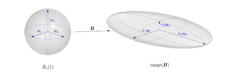
        (a) Geometry of the SVD. The linear map $\bm{B}\in\mathbb{R}^{n\times m}$ transforms the unit sphere in $\mathbb{R}^{n}$ to an ellipsoid in $\mathbb{R}^{m}$ with semiaxes determined by the singular values and the singular vectors of $\bm{B}$.

        

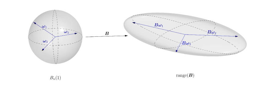
        (b) Images of random vectors. A normalized Gaussian vector $\bm{\omega}/\|{\bm{\omega}}\|_{2}$ is distributed uniformly on the unit sphere. The image $\bm{B}\bm{\omega}$ tends to align with the major semiaxes of the ellipsoid defined by $\bm{B}$. To cover the leading $r$ directions, we need to use slightly more than $r$ random test vectors.

        Figure 3.1. Randomized SVD: Intuition. These schematics illustrate the geometric ideas behind the SVD and the randomized SVD.

        What can we say about the optimal low-rank approximation of the matrix $\bm{B}$? Given a rank parameter $r\leq\min\{m,n\}$, define the orthogonal projector $\bm{P}_{r}$ onto the span of the leading $r$ left singular vectors:

        $$\bm{P}_{r}\coloneqq\sum_{i=1}^{r}\bm{u}_{i}\bm{u}_{i}^{*}.$$

        The Eckart–Young theorem [EY36:Approximation-One] identifies the best rank-$r$ approximation with respect to the Frobenius norm:

        $$\min\nolimits_{\operatorname{rank}(\bm{M})\leq r}\|{\bm{B}-\bm{M}}\|_{\mathrm{F}}^{2}=\|{\bm{B}-\bm{P}_{r}\bm{B}}\|_{\mathrm{F}}^{2}=\sum_{i>r}\sigma_{i}^{2}.$$ (3.9)

        In words, the best approximation is achieved by projecting the target matrix onto the $r$-dimensional subspace that captures most of the action of the matrix. Throughout this discussion, we focus on the Frobenius-norm error to obtain more transparent results.

        In some applications, it is unnecessary to compute the best approximation to high accuracy. Instead, we can relax our requirements. Let $s=r+\ell$ for a small natural number $\ell$. For a tolerance $\varepsilon>0$, we seek a rank-$s$ approximation $\widehat{\bm{B}}_{s}$ that competes with the best rank-$r$ approximation (3.9):

        $$\|{\bm{B}-\widehat{\bm{B}}_{s}}\|_{\mathrm{F}}^{2}\leq(1+\varepsilon)\cdot\|{\bm{B}-\bm{P}_{r}\bm{B}}\|_{\mathrm{F}}^{2}=(1+\varepsilon)\cdot\sum_{i>r}\sigma_{i}^{2}.$$ (3.10)

        When the best rank-$r$ approximation error is tiny, it is not a big deal to pay a modest factor $(1+\varepsilon)$ more. This situation occurs in scientific computing applications where the singular values of the matrix decay exponentially fast [HMT11:Finding-Structure, Sec. 7.1].

        3.2.2. Randomized SVD: Intuition

        Our goal is to produce an estimate for the best rank-$r$ approximation $\bm{P}_{r}\bm{B}$ of the input matrix. Instead of computing the projector $\bm{P}_{r}$ onto the $r$ leading left singular vectors, we will use randomness to estimate these directions. We can trace this insight to work of Frieze et al. [FKV98:Fast-Monte-Carlo]. Martinsson et al. [MRT06:Randomized-Algorithm] developed this idea into a practical algorithm, which was crystallized in the paper [HMT11:Finding-Structure].

        The method is to multiply random test vectors into the matrix $\bm{B}$ to identify salient directions. We have the intuition that the image of a random vector tends to be aligned with the leading left singular vectors. By repetition, we can cover most of the significant directions in the range of the projector $\bm{P}_{r}$. Since we do not know the orthonormal basis of right singular vectors, it is natural to draw the random vectors from a rotationally invariant distribution. See Figure 3.1(b) for an illustration.

        We can describe this approach mathematically [TW23:Randomized-Algorithms, Sec. 2.1]. Draw a standard normal test vector $\bm{\omega}\in\mathbb{R}^{n}$. The image of the random vector satisfies

        $$\bm{B}\bm{\omega}=\sum_{i=1}^{m\wedge n}\sigma_{i}\,\bm{u}_{i}(\bm{v}_{i}^{*}\bm{\omega})\eqqcolon\sum_{i=1}^{m\wedge n}\omega_{i}\sigma_{i}\,\bm{u}_{i}$$

        As before, the component $\omega_{i}\coloneqq\bm{v}_{i}^{*}\bm{\omega}$ of the random vector along the $i$th right singular vector follows a standard normal distribution, and the components $(\omega_{i}:i=1,\dots,m\wedge n)$ compose an independent family. On average, $\operatorname{\mathbb{E}}[\omega_{i}^{2}]=1$. Therefore, the image $\bm{B}\bm{\omega}$ tends to align with the left singular vectors associated with large singular values.

        By repeating this process with a statistically independent family $(\bm{\omega}^{(j)}:j=1,\dots,s)$ of random test vectors, we can obtain a family $(\bm{B}\bm{\omega}^{(j)}:j=1,\dots,s)$ of vectors whose span contains most of ${P}_{r})$. The number $s=r+\ell$ of test vectors needs to be a bit larger than the target rank $r$ to obtain coverage of the subspace with high probability.

        3.2.3. Randomized SVD: Algorithm

        Let us forge this intuition into an algorithm [HMT11:Finding-Structure, p. 227], called the randomized SVD. For a rank parameter $s$, we draw a random test matrix:

        $$\bm{\Omega}=\begin{bmatrix}\bm{\omega}^{(1)}&\dots&\bm{\omega}^{(s)}\end{bmatrix}\in\mathbb{R}^{n\times s}\quad\text{where $\bm{\omega}^{(j)}\sim\textsc{normal}(\bm{0},\mathbf{I}_{n})$ i.i.d.}$$

        We obtain the images of the test vectors using a matrix–matrix product with the input matrix:

        $$\bm{Y}\coloneqq\bm{B\Omega}.$$

        This step requires $s$ matvecs with $\bm{B}$. The orthogonal projector $\bm{P}_{\bm{Y}}$ onto the range of $\bm{Y}$ serves as a proxy for the ideal projector $\bm{P}_{r}$. Computationally,

        $$\bm{P}_{\bm{Y}}\coloneqq\bm{QQ}^{*}\quad\text{where}\quad\bm{Q}\coloneqq\texttt{orth}(\bm{Y}).$$

        The function orth returns an orthonormal basis for the range of a matrix, and it costs $\mathcal{O}(s^{2}m)$ arithmetic operations. Finally, we report the approximation $\widehat{\bm{B}}_{s}$ in factored form:

        $$\widehat{\bm{B}}_{s}\coloneqq\bm{P}_{\bm{Y}}\bm{B}=\bm{Q}(\bm{Q}^{*}\bm{B})$$

        This step requires $s$ matvecs with the transpose $\bm{B}^{*}$. If desired, we can report the SVD of the approximation after a small amount of additional work:

        $$\widehat{\bm{B}}_{s}=(\bm{Q}\widehat{\bm{U}}_{0})\widehat{\bm{\Sigma}}\widehat{\bm{V}}^{*}\quad\text{where}\quad(\widehat{\bm{U}}_{0},\widehat{\bm{\Sigma}},\widehat{\bm{V}})=\texttt{svd}(\bm{Q}^{*}\bm{B}).$$

        This step costs another $\mathcal{O}(s^{2}n)$ arithmetic operations.

        See Algorithm 4 for pseudocode for the randomized SVD algorithm. For a dense unstructured matrix $\bm{B}$, the total cost is $\mathcal{O}(smn)$. To compare, recall that a dense, economy-size SVD costs $\mathcal{O}(mn(m\wedge n))$. Classic Krylov subspace methods are competitive in cost with the randomized SVD, but they often fail for challenging problem instances [LLS+17:Algorithm-971]. In contrast, the randomized SVD and its relatives are bulletproof.

        1Input matrix $\bm{B}\in\mathbb{R}^{m\times n}$, number $s$ of samples

        2Factors $\bm{Q}\in\mathbb{R}^{m\times s}$ and $\bm{C}\in\mathbb{R}^{s\times n}$ of the approximation $\widehat{\bm{B}}_{s}=\bm{QC}$  

        3function RandSVD($\bm{B}$)

        4     Sample $\bm{\Omega}\sim\textsc{normal}(\bm{0},\mathbf{I}_{m}\otimes\mathbf{I}_{n})\in\mathbb{R}^{m\times n}$ $\triangleright$ Standard normal test matrix

        5     $\bm{Y}=\bm{B}\bm{\Omega}$ $\triangleright$ $s$ matvecs with $\bm{B}$

        6     $\bm{Q}=\texttt{orth}(\bm{Y})$ $\triangleright$ Orthonormal basis for range of $\bm{Y}$

        7     $\bm{C}=\bm{Q}^{*}\bm{B}$ $\triangleright$ $s$ matvecs with $\bm{B}^{*}$

        8     $(\widehat{\bm{U}}_{0},\widehat{\bm{\Sigma}},\widehat{\bm{V}})=\texttt{svd}(\bm{C})$ $\triangleright$ Optional: Report SVD of approximation

        9     $\widehat{\bm{U}}=\bm{Q}\widehat{\bm{U}}_{0}$ $\triangleright$ $\widehat{\bm{B}}_{s}=\widehat{\bm{U}}\widehat{\bm{\Sigma}}\widehat{\bm{V}}^{*}$

        Algorithm 4 Randomized SVD.

        3.2.4. Randomized SVD: Analysis

        Concerning the randomized SVD, the main question is how many test vectors $s$ are needed to obtain a rank-$r$ approximation that satisfies (3.10). We present a result from Halko et al. [HMT11:Finding-Structure, Thm. 10.5] that accurately predicts the performance of the randomized SVD algorithm.

        Theorem 3.6 (Randomized SVD; Halko et al. 2011).

        Consider a matrix $\bm{B}\in\mathbb{R}^{m\times n}$, and fix the target rank $r\leq m\wedge n$. When $s\geq r+2$, the randomized SVD method (Algorithm 4) produces a random rank-$s$ approximation $\widehat{\bm{B}}_{s}$ that satisfies

        $$\operatorname{\mathbb{E}}\|{\bm{B}-\widehat{\bm{B}}_{s}}\|_{\mathrm{F}}^{2}\leq\left(1+\frac{r}{s-r-1}\right)\cdot\sum_{i>r}\sigma^{2}_{i}(\bm{B}).$$ (3.11)

        On average, to obtain a tolerance $\varepsilon>0$ in the error bound (3.10), it suffices that $s=1+r+r/\varepsilon$.

        This theorem places no restrictions on the input matrix (such as a spectral gap). To unpack the result, recall that the sum $\sum_{i>r}\sigma_{i}^{2}$ on the right-hand side of (3.11) is the Eckart–Young error (3.9) in the best rank-$r$ approximation. The factor $\varepsilon=r/(s-r-1)$ reflects the loss that we suffer from constructing the approximation $\widehat{\bm{B}}_{s}$ using the random projector $\bm{P}_{\bm{Y}}$ instead of the ideal projector $\bm{P}_{r}$. By increasing the number $s$ of samples, we can drive the error tolerance $\varepsilon$ down as far as we like. In particular, $s=2r+1$ yields a tolerance $\varepsilon=1$. This type of approximation might seem too weak to be useful. But keep in mind that the main use case for the randomized SVD algorithm is when the optimal error is tiny because the singular values decay exponentially [HMT11:Finding-Structure, TW23:Randomized-Algorithms].

        We will sketch the proof of Theorem 3.6 to show how the properties of the random test matrix $\bm{\Omega}$ enter into the bound. As with the randomized power method, the key insight is that the random test matrix $\bm{\Omega}$ aligns reasonably well with the leading right singular vectors of the input matrix $\bm{B}$. At the same time, the test matrix does not align too strongly with the trailing right singular vectors. To quantify these properties, we depend on some basic facts from random matrix theory.

        As an aside, results like Theorem 3.6 also hold for the spectral-norm error [HMT11:Finding-Structure, Thm. 10.6], but the proof requires some technical arguments that do not contribute new insight about the mechanism that drives the randomized SVD algorithm.

        Proof of Theorem 3.6.

        Fix the target rank $r\leq m\wedge n$ and the number $s$ of random test vectors. We can express the SVD (3.8) of the input matrix $\bm{B}$ in block matrix form to isolate the leading $r$ singular directions:

        $$\bm{B}=\begin{bmatrix}\bm{U}_{r}&\bm{U}_{\perp}\end{bmatrix}\begin{bmatrix}\bm{\Sigma}_{r}&\bm{0}\\ \bm{0}&\bm{\Sigma}_{\perp}\end{bmatrix}\begin{bmatrix}\bm{V}_{r}&\bm{V}_{\perp}\end{bmatrix}^{*}.$$

        Explicitly, $\bm{U}_{r}\in\mathbb{R}^{m\times r}$, and $\bm{\Sigma}_{r}=\operatorname{diag}(\sigma_{1},\dots,\sigma_{r})$, and $\bm{V}_{r}\in\mathbb{R}^{n\times r}$.

        Next, extract the components of the test matrix $\bm{\Omega}$ in the basis of right singular vectors:

        $$\bm{\Omega}_{r}\coloneqq\bm{V}_{r}^{*}\bm{\Omega}\quad\text{and}\quad\bm{\Omega}_{\perp}\coloneqq\bm{V}_{\perp}^{*}\bm{\Omega}.$$

        This decomposition is similar to the one we used to analyze the power method. The matrix $\bm{\Omega}_{r}$ describes the alignment of the test matrix with the leading right singular vectors, while $\bm{\Omega}_{\perp}$ describes the alignment with the trailing right singular vectors.

        After some linear algebra (omitted), we can develop the following (deterministic) bound for the approximation error [HMT11:Finding-Structure, Thm. 9.1]. For a streamlined proof, see [TW23:Randomized-Algorithms, Prop. 8.5].

        Proposition 3.7 (Randomized SVD: Approximation error).

        With notation as above, assume that $\operatorname{rank}(\bm{\Omega}_{r})=r$. Then the rank-$s$ approximation $\widehat{\bm{B}}_{s}$ produced by Algorithm 4 satisfies

        $$\|{\bm{B}-\widehat{\bm{B}}_{s}}\|_{\mathrm{F}}^{2}\leq\|{\bm{\Sigma}_{\perp}}\|_{\mathrm{F}}^{2}+\|{\bm{\Sigma}_{\perp}\bm{\Omega}_{\perp}\bm{\Omega}_{r}^{\dagger}}\|_{\mathrm{F}}^{2}$$ (3.12)

        The first term on the right-hand side of (3.12) reflects the trailing singular values of the matrix. Every rank-$r$ approximation (3.9) suffers this loss. The second term is the deficit from using the test matrix $\bm{\Omega}$. We want the component $\bm{\Omega}_{r}$ in the leading directions to be well conditioned (ideally, an identity matrix). We want the component $\bm{\Omega}_{\perp}$ in the trailing directions to be as small as possible.

        It is instructive to compare Proposition 3.7 with the error bound (3.7) for the power method when $t=1$. Indeed, the quantity $\|{\bm{\Omega}_{r}^{\dagger}}\|_{\mathrm{F}}^{2}$ is analogous to the term $\omega_{1}^{2}$ in the denominator of (3.7). Meanwhile, the quantity $\|{\bm{\Sigma}_{\perp}\bm{\Omega}_{\perp}}\|_{\mathrm{F}}^{2}$ is analogous with the sum $\sum_{i>1}\omega_{i}^{2}\lambda_{i}^{2}$ in the numerator of (3.7).

        Now, we can exploit the rotational invariance of the standard normal test matrix $\bm{\Omega}$ to evaluate the expectation of the error bound (3.12). Note that the columns of the leading singular vectors $\bm{V}_{r}$ and the trailing singular vectors $\bm{V}_{\perp}$ are mutually orthogonal. Therefore, the associated components $\bm{\Omega}_{r}\in\mathbb{R}^{r\times s}$ and $\bm{\Omega}_{\perp}\in\mathbb{R}^{(n-r)\times s}$ of the test matrix are standard normal matrices that are statistically independent. In particular, if $s\geq r$, then $\operatorname{rank}(\bm{\Omega}_{r})=r$ with probability one. This holds true regardless of the right singular vectors of $\bm{B}$.

        To evaluate the expected deficit in the error bound (3.12), we use independence to introduce conditional expectations. Thus,

        $$\operatorname{\mathbb{E}}\|{\bm{\Sigma}_{\perp}\bm{\Omega}_{\perp}\bm{\Omega}_{r}^{\dagger}}\|_{\mathrm{F}}^{2}=\operatorname{\mathbb{E}}_{\bm{\Omega}_{r}}\big{[}\operatorname{\mathbb{E}}_{\bm{\Omega}_{\perp}}\|{\bm{\Sigma}_{\perp}\bm{\Omega}_{\perp}\bm{\Omega}_{r}^{\dagger}}\|_{\mathrm{F}}^{2}\big{]}=\operatorname{\mathbb{E}}_{\bm{\Omega}_{r}}\big{[}\|{\bm{\Sigma}_{\perp}}\|_{\mathrm{F}}^{2}\cdot\|{\bm{\Omega}_{r}^{\dagger}}\|_{\mathrm{F}}^{2}\big{]}.$$

        The second identity follows when we write out the Frobenius norm in coordinates and find the expectation over the entries of $\bm{\Omega}_{\perp}$ by direct calculation. The Frobenius norm of the remaining random matrix can be rewritten as a trace:

        $$\operatorname{\mathbb{E}}_{\bm{\Omega}_{r}}\|{\bm{\Omega}_{r}^{\dagger}}\|_{\mathrm{F}}^{2}=\operatorname{\mathbb{E}}_{\bm{\Omega}_{r}}\operatorname{tr}\big{[}(\bm{\Omega}_{r}\bm{\Omega}_{r}^{*})^{-1}\big{]}=\frac{r}{s-r-1}.$$

        Indeed, since $\bm{\Omega}_{r}\in\mathbb{R}^{r\times s}$ is standard normal, the product $\bm{W}=\bm{\Omega}_{r}\bm{\Omega}_{r}^{*}$ follows the standard $\textsc{wishart}(s,\mathbf{I}_{r})$ distribution with $s$ degrees of freedom. The calculation of $\operatorname{\mathbb{E}}\operatorname{tr}[\bm{W}^{-1}]$ is a classical result from statistics [HMT11:Finding-Structure, Prop. A.6].

        To conclude, take the expectation of (3.12), and introduce the last two displays:

        $$\operatorname{\mathbb{E}}\|{\bm{B}-\widehat{\bm{B}}_{s}}\|_{\mathrm{F}}^{2}\leq\|{\bm{\Sigma}_{\perp}}\|_{\mathrm{F}}^{2}+\operatorname{\mathbb{E}}\|{\bm{\Sigma}_{\perp}\bm{\Omega}_{\perp}\bm{\Omega}_{r}^{\dagger}}\|_{\mathrm{F}}^{2}\leq\left(1+\frac{r}{s-r-1}\right)\cdot\|{\bm{\Sigma}_{\perp}}\|_{\mathrm{F}}^{2}.$$

        Last, we recognize $\|{\bm{\Sigma}_{\perp}}\|_{\mathrm{F}}^{2}$ as the sum of the squares of the trailing singular values of $\bm{B}$. ∎

        3.2.5. Discussion

        We have shown that the random choice of test matrix plays an integral role in the randomized SVD algorithm for low-rank matrix approximation. This example may seem different in spirit from the randomized initialization for the power method, but the algorithms are actually close relatives.

        Indeed, we can extend the randomized SVD to an algorithm called randomized subspace iteration by repeated multiplication with the test matrix:

        1. Sample $\bm{\Omega}=\begin{bmatrix}\bm{\omega}^{(1)}&\dots&\bm{\omega}^{(s)}\end{bmatrix}\in\mathbb{R}^{n\times s}$ with i.i.d. standard normal columns.

        2. Set the initial iterate $\bm{X}_{0}=\bm{\Omega}$.

        3. For $t=1,2,3,\dots,T$, compute

           $$\bm{Q}_{t}\coloneqq\texttt{orth}(\bm{B}\bm{X}_{t-1})\quad\text{and}\quad\bm{X}_{t}\coloneqq\bm{B}^{*}\bm{Q}_{t}$$

        4. Return the approximation $\widehat{\bm{B}}_{s}=\bm{Q}_{T}\bm{X}_{T}^{*}$.

           The randomized SVD (Algorithm 4) is the special case of this procedure with $T=1$.

           Unrolling the recurrence, we find that randomized subspace iteration produces approximations

           $$\widehat{\bm{B}}_{s}=\bm{Q}_{t}(\bm{Q}_{t}^{*}\bm{B})\quad\text{where}\quad\bm{Q}_{t}=\texttt{orth}((\bm{BB}^{*})^{t-1}\bm{B}\bm{\Omega})\quad\text{for $t=1,2,3,\dots$.}$$

           Much as the power method drives its iterates toward the leading eigenspace, subspace iteration drives ${Q}_{t})$ so that it aligns with ${U}_{r})$, the leading left singular subspace of $\bm{B}$. The random starting matrix $\bm{\Omega}$ has sufficient alignment with the leading right singular vectors $\bm{V}_{r}$ to begin this process. Meanwhile, the starting matrix $\bm{\Omega}$ is oblique with the trailing right singular vectors $\bm{V}_{\perp}$, so they do not interfere too much with the convergence. See [HMT11:Finding-Structure, TW23:Randomized-Algorithms] for the analysis of randomized subspace iteration.

           We can also study randomized block Lanczos methods for low-rank matrix approximation [RST09:Randomized-Algorithm, HMST11:Algorithm-Principal, MM15:Randomized-Block]. These algorithms exhibit much faster convergence than randomized subspace iteration, so they are especially valuable for matrices whose singular values decay very slowly. For these methods too, the random starting matrix is a critical ingredient. See [TW23:Randomized-Algorithms] for a recent survey.

           4. Progress on average

           In the last section, we considered algorithms that start from a random initialization and drive this point toward a solution to the computational problem. Of course, there is no reason to limit the role of probability to the initialization. This section introduces another template where we make random choices at each step of an iterative algorithm. The methods we study share the feature that each step reduces the error (or some other measure of progress) on average.

           Theme (Progress on average).

           At each step of an (iterative) algorithm, make a random choice so that the expected error decreases.

           In optimization, a familiar example of this template is stochastic gradient iteration [Bot10:Large-Scale-Machine]. This is a randomized variant of gradient descent in which the gradient is replaced by an unbiased random estimate that is cheaper to compute. Just as a small step in the direction of the negative gradient reduces the value of the objective function, a step in the direction of the random gradient estimate reduces the objective value on average. Even if the individual gradient estimates are very poor, we can still guarantee convergence of the randomized algorithm.

           We will study two problems in numerical linear algebra that we can tackle using randomized algorithms that make progress on average. First, we study the randomized Kaczmarz iteration for solving an overdetermined least-squares problem. Second, we describe the randomly pivoted partial Cholesky method for computing a low-rank approximation of a psd matrix.

           4.1. Randomized Kaczmarz

           Another classic linear algebra problem, dating to the time of Gauss, is the linear least-squares problem, often used for fitting linear models to data. We will focus on the overdetermined setting where the number of observations (dramatically) exceeds the number of variables in the model. This problem arises in a range of applications, such as statistical estimation, signal processing, machine learning, and even as a subroutine in other linear algebra and optimization computations.

           Problem (Overdetermined least-squares).

           Given a tall matrix $\bm{A}\in\mathbb{R}^{n\times d}$ with $n\gg d$ and a response vector $\bm{b}\in\mathbb{R}^{n}$, find a solution to the overdetermined least-squares problem:

           $${{\textsf{minimize}}}_{\bm{x}\in\mathbb{R}^{d}}\quad\tfrac{1}{2}\|{\bm{A}\bm{x}-\bm{b}}\|^{2}_{2}.$$

           For large-scale instances, it may not be desirable or even feasible to tackle the least-squares problem using direct methods, which cost $\mathcal{O}(d^{2}n)$ arithmetic operations. Instead, we can seek iterative algorithms that approximate the solution at a lower computational cost. In particular, we will study methods that enforce individual equations. We will see that enforcing a randomly chosen equation leads to a simple, elegant algorithm with nice convergence guarantees.

           4.1.1. The Kaczmarz iteration

           There are many iterative methods for solving least-squares problems. Let us introduce a classic algorithm, attributed to Kaczmarz [Kac37:Angenaherte]. This method has historically been popular for computed tomography and digital signal processing applications [SV09:Randomized-Kaczmarz].

           Consider a tall matrix $\bm{A}\in\mathbb{R}^{n\times d}$ with $n\gg d$, and write $\bm{a}_{i}^{*}$ for the $i$th row of the matrix. Choose a response vector $\bm{b}=(b_{1},\dots,b_{n})^{*}\in\mathbb{R}^{n}$. We can frame the overdetermined least-squares problem as

           $${{\textsf{minimize}}}_{\bm{x}\in\mathbb{R}^{d}}\quad\frac{1}{2}\sum_{i=1}^{n}\big{(}\langle{\bm{a}_{i}},\ {\bm{x}}\rangle-b_{i}\big{)}^{2}.$$ (4.1)

           As usual, $\langle{\cdot},\ {\cdot}\rangle$ denotes the standard inner product on $\mathbb{R}^{d}$. Each term $i=1,\dots,n$ in the sum corresponds to the squared residual in a single equation, and we can develop algorithms that work with the individual equations.

           The Kaczmarz iteration begins with an initial iterate $\bm{x}_{0}\in\mathbb{R}^{d}$, often taken to be the zero vector. At each iteration $t=1,2,3,\dots$, we select an equation $j(t)$ and update the previous iterate $\bm{x}_{t-1}$ so this equation holds exactly:

           $$\bm{x}_{t}=\bm{x}_{t-1}-\frac{\langle{\bm{a}_{j(t)}},\ {\bm{x}_{t-1}}\rangle-b_{j(t)}}{\|{\bm{a}_{j(t)}}\|_{2}^{2}}\cdot\bm{a}_{j(t)}\quad\text{for $t=1,2,3,\dots$.}$$ (4.2)

           A short calculation confirms that $\langle{\bm{a}_{j(t)}},\ {\bm{x}_{t}}\rangle=b_{j(t)}$. Each iteration of the Kaczmarz method costs just $\mathcal{O}(d)$ operations, irrespective of the number $n$ of equations. As an aside, note that the update amounts to a step in the direction of the gradient of the $i$th squared residual in (4.1), so we can interpret the Kaczmarz iteration as a type of gradient descent method.

           To design a Kaczmarz algorithm, we need to specify a control rule $j(t)$ for picking the equation at iteration $t$. In the classical literature, it was most common to repeatedly cycle through the equations in the order given. Another alternative is to arrange the equations in random order and cycle through them. A third possibility is to enforce the equation that has the largest residual, although this rule can be expensive to implement. These strategies all lead to convergent algorithms, but it is challenging to understand the rate of convergence because it depends in a complicated way on the problem data and the control rule.

           4.1.2. The role of randomness

           To address the limitations of the classic Kaczmarz method, Strohmer & Vershynin [SV09:Randomized-Kaczmarz] proposed a variant that uses a randomized control rule. Their idea is that we can make progress on average toward the solution if we select an equation at random at each step. To control the variability of the randomized algorithm, the sampling probabilities should also reflect the “importance” of each equation.

           With this preface in mind, we describe a random control rule for the Kaczmarz method. At each iteration $t$, the random row $J(t)$ is drawn independently from all previous random choices $(J(1),\dots,J(t-1))$. The distribution of the random row $J(t)$ takes the form

           $$\mathbb{P}\left\{J(t)=i\right\}=\frac{\|{\bm{a}_{i}}\|^{2}_{2}}{\|{\bm{A}}\|_{\mathrm{F}}^{2}}\quad\text{for $i=1,\dots,n$.}$$ (4.3)

           In other words, the “importance” of an equation to the least-squares problem (4.1) is proportional to its squared norm, for reasons that will become clear in the analysis. We already encountered a similar distribution in our discussion of approximate matrix multiplication (Section 2.2.3). This is an instance of importance sampling, a variance reduction technique that was developed in the Monte Carlo approximation literature.

           Algorithm 5 lists the pseudocode for this randomized Kaczmarz method. Note that it takes $\mathcal{O}(dn)$ operations to compute the sampling probabilities exactly. Each iteration requires $\mathcal{O}(d)$ operations.

           1Matrix $\bm{A}\in\mathbb{R}^{n\times d}$, response $\bm{b}\in\mathbb{R}^{n}$, initial iterate $\bm{x}_{0}\in\mathbb{R}^{d}$, number $T$ of iterations

           2Solution estimate $\bm{x}_{T}\in\mathbb{R}^{d}$  

           3function RandKaczmarz($\bm{A}$, $\bm{b}$; $\bm{x}_{0}$)

           4     $r_{i}=\|{\bm{a}_{i}}\|_{2}^{2}$ for $i=1,\dots,n$ $\triangleright$ $\bm{a}_{i}^{*}$ is $i$th row of matrix

           5     $p_{i}=r_{i}/\sum_{j=1}^{n}r_{j}$ $\triangleright$ Sampling probabilities

           6     for $t=1,2,3,\dots,T$ do

           7         Sample row index $j(t)$ from distribution $(p_{i}:i=1,\dots,n)$

           8         $\bm{x}_{t}=\bm{x}_{t-1}-(\langle{\bm{a}_{j(t)}},\ {\bm{x}_{t-1}}\rangle-b_{i})\bm{a}_{j(t)}/\|{\bm{a}_{j(t)}}\|^{2}_{2}$ $\triangleright$ Update iterate      

           Algorithm 5 Randomized Kaczmarz.

           4.1.3. Randomized Kaczmarz: Analysis

           In this section, we give an elegant analysis of the randomized Kaczmarz iteration due to Strohmer & Vershynin [SV09:Randomized-Kaczmarz]. Following their presentation, we assume that $\bm{A}$ is injective and that the least-squares problem is consistent: $\bm{b}\in{A})$. Under these extra hypotheses, the least-squares problem admits a unique solution $\bm{x}_{\star}\in\mathbb{R}^{d}$ that is exact: $\bm{A}\bm{x}_{\star}=\bm{b}$. Thus, we can measure progress of the iterates toward the solution:

           $$\|{\bm{x}_{t}-\bm{x}_{\star}}\|^{2}_{2}\quad\text{for $t=0,1,2,\dots$.}$$

           We will prove that, on average, the randomized control rule (4.3) reduces the squared norm of the error by a constant factor at each iteration.

           The analysis shows that the convergence factor of the randomized Kaczmarz method depends on the Demmel condition number [Dem88:Probability-Numerical] of the matrix:

           $$\kappa_{\mathrm{dem}}\coloneqq\kappa_{\mathrm{dem}}(\bm{A})\coloneqq\frac{\|{\bm{A}}\|_{\mathrm{F}}}{\sigma_{\min}(\bm{A})}.$$ (4.4)

           Here, $\sigma_{\min}(\bm{A})$ is the $d$th largest singular value of the matrix $\bm{A}\in\mathbb{R}^{n\times d}$. For comparison, recall the standard condition number $\kappa\coloneqq\sigma_{\max}/\sigma_{\min}$ for linear systems. We have the inequalities $\kappa\leq\kappa_{\mathrm{dem}}\leq\sqrt{d}\kappa$ for every matrix with $d$ columns. Much as the intrinsic dimension refines the notion of the rank of a psd matrix, the Demmel condition number $\kappa_{\mathrm{dem}}$ accounts for the number of energetic directions in the range of the matrix, whereas the standard condition number $\kappa$ does not.

           Theorem 4.1 (Randomized Kaczmarz; Strohmer & Vershynin 2009).

           Consider a consistent system of linear equations $\bm{A}\bm{x}=\bm{b}$ where $\bm{A}$ is injective, and let $\bm{x}_{\star}$ be the (unique) solution. For each $t=1,2,3,\dots$, the randomized Kaczmarz iteration (Algorithm 5) yields the error bound

           $$\operatorname{\mathbb{E}}\|{\bm{x}_{t}-\bm{x}_{\star}}\|^{2}_{2}\leq\big{(}1-\kappa_{\mathrm{dem}}^{-2}\big{)}^{t}\cdot\|{\bm{x}_{0}-\bm{x}_{\star}}\|^{2}_{2}.$$

           Before turning to the proof, let us discuss what this result means [SV09:Randomized-Kaczmarz, Sec. 2.1]. For a tolerance $\varepsilon>0$, we can bound the expected number of iterations that suffice to drive the error below the tolerance.

           $$T\geq 2\kappa_{\mathrm{dem}}^{2}\log(1/\varepsilon)\quad\text{implies}\quad\operatorname{\mathbb{E}}\|{\bm{x}_{T}-\bm{x}_{\star}}\|^{2}_{2}\leq\varepsilon^{2}\|{\bm{x}_{0}-\bm{x}_{\star}}\|_{2}.$$

           Suppose that the standard condition number $\kappa$ is a constant that does not depend on the matrix dimensions. Then $\kappa_{\mathrm{dem}}^{2}=\mathcal{O}(d)$. We determine that $T=\mathcal{O}(d\log(1/\varepsilon))$ iterations suffice to obtain $\varepsilon$-error, relative to the initial guess. If the sampling probabilities are given, then the cost of the whole algorithm is just $\mathcal{O}(d^{2}\log(1/\varepsilon))$ operations, in contrast to the $\mathcal{O}(nd^{2})$ cost of a direct method. Indeed, we may not even need to enforce all of the equations!

           Proof of Theorem 4.1.

           We begin with a short linear algebra calculation that describes the evolution of the error in the deterministic Kaczmarz iteration. Since $\bm{x}_{\star}$ satisfies the linear equations, we have $\langle{\bm{a}_{i}},\ {\bm{x}_{\star}}\rangle=b_{i}$ for each row $i$. For each iteration $t=0,1,2,\dots$, define the error vector $\bm{e}_{t}\coloneqq\bm{x}_{t}-\bm{x}_{\star}$. The Kaczmarz update (4.2) ensures that the error vector satisfies

           $$\bm{e}_{t}\coloneqq\bm{x}_{t}-\bm{x}_{\star} =(\bm{x}_{t-1}-\bm{x}_{\star})-\frac{\langle{\bm{a}_{j(t)}},\ {\bm{x}_{t-1}-\bm{x}_{\star}}\rangle}{\|{\bm{a}_{j(t)}}\|^{2}_{2}}\cdot\bm{a}_{j(t)}$$

           $$=\bm{e}_{t-1}-\frac{\bm{a}_{j(t)}\bm{a}_{j(t)}^{*}}{\|{\bm{a}_{j}}\|^{2}_{2}}\cdot\bm{e}_{t-1}\eqqcolon\big{(}\mathbf{I}-\bm{P}_{j(t)}\big{)}\bm{e}_{t-1}.$$

           For each row index $i$, we define the orthogonal projector $\bm{P}_{i}\coloneqq\bm{a}_{i}\bm{a}_{i}^{*}/\|{\bm{a}_{i}}\|^{2}_{2}$ onto the span of $\bm{a}_{i}$. Taking the squared norm of the error evolution equation,

           $$\|{\bm{e}_{t}}\|^{2}_{2}=\|{\big{(}\mathbf{I}-\bm{P}_{j(t)}\big{)}\bm{e}_{t-1}}\|^{2}_{2}=\left\langle{\bm{e}_{t-1}},\ {\big{(}\mathbf{I}-\bm{P}_{j(t)}\big{)}\bm{e}_{t-1}}\right\rangle.$$ (4.5)

           We can bound the reduction in the error by understanding how much the projection onto the row $j(t)$ cuts down the residual. When $j(t)$ is deterministic, this argument is challenging.

           Instead, we implement the randomized control rule (4.3). In this case, the projector $\bm{P}_{J(t)}$ is a random matrix. Averaging with respect to the randomness in $J(t)$,

           $$\operatorname{\mathbb{E}}_{J(t)}[\bm{P}_{J(t)}]=\sum_{i=1}^{n}\bm{P}_{i}\cdot\mathbb{P}\left\{J(t)=i\right\}=\sum_{i=1}^{n}\frac{\bm{a}_{i}\bm{a}_{i}^{*}}{\|{\bm{a}_{i}}\|^{2}_{2}}\cdot\frac{\|{\bm{a}_{i}}\|^{2}_{2}}{\|{\bm{A}}\|_{\mathrm{F}}^{2}}=\frac{1}{\|{\bm{A}}\|_{\mathrm{F}}^{2}}\bm{A}^{*}\bm{A}.$$

           The importance sampling distribution for the row index is designed to cancel out the squared norms. As a consequence, the expected projector is proportional to the Gram matrix $\bm{A}^{*}\bm{A}$, so the convergence rate of the randomized Kaczmarz method will reflect the geometric properties of the input matrix $\bm{A}$.

           Taking the expectation of (4.5) and exploiting linearity,

           $$\operatorname{\mathbb{E}}_{J(t)}\|{\bm{e}_{t}}\|^{2}_{2} =\left\langle{\bm{e}_{t-1}},\ {\big{(}\mathbf{I}-\operatorname{\mathbb{E}}_{J(t)}[\bm{P}_{J(t)}]\big{)}\bm{e}_{t-1}}\right\rangle=\left\langle{\bm{e}_{t-1}},\ {\big{(}\mathbf{I}-\|{\bm{A}}\|_{\mathrm{F}}^{-2}\bm{A}^{*}\bm{A}\big{)}\bm{e}_{t-1}}\right\rangle$$

           $$\leq\lambda_{1}\big{(}\mathbf{I}-\|{\bm{A}}\|_{\mathrm{F}}^{-2}\bm{A}^{*}\bm{A}\big{)}\cdot\|{\bm{e}_{t-1}}\|^{2}_{2}=\left(1-\frac{\sigma_{\min}(\bm{A})^{2}}{\|{\bm{A}}\|_{\mathrm{F}}^{2}}\right)\cdot\|{\bm{e}_{t-1}}\|^{2}_{2}.$$

           Recalling the definition (4.4) of the Demmel condition number, we reach

           $$\operatorname{\mathbb{E}}_{J(t)}\|{\bm{e}_{t}}\|^{2}_{2}\leq\big{(}1-\kappa_{\mathrm{dem}}^{-2}\big{)}\cdot\|{\bm{e}_{t-1}}\|^{2}_{2}.$$ (4.6)

           At each iteration, the randomized Kaczmarz method makes progress on average. Finally, we take the total expectation using the tower rule and the independence of control sequence:

           $$\operatorname{\mathbb{E}}\|{\bm{e}_{t}}\|^{2}_{2}\leq\big{(}1-\kappa_{\mathrm{dem}}^{-2}\big{)}\cdot\operatorname{\mathbb{E}}\|{\bm{e}_{t-1}}\|^{2}_{2}.$$

           Unrolling this recurrence, we obtain the stated result. ∎

           The proof hinges on the formula (4.6), which states that the error sequence $(\|{\bm{e}_{t}}\|^{2}_{2}:t=0,1,2,\dots)$ composes a positive supermartingale. This observation has some striking implications for the long-term behavior of the randomized Kaczmarz method [CP12:Almost-Sure-Convergence]. In particular, a standard argument using the Borel–Cantelli lemma provides that

           $$(1-\varrho)^{-t}\cdot\|{\bm{e}_{t}}\|^{2}_{2}\to 0\quad\text{almost surely for each $\varrho<\kappa_{\mathrm{dem}}^{-2}$.}$$

           We can also obtain uniform concentration inequalities for the error sequence by an application of Ville’s inequality [Tro23:Probability-Theory-LN, Thm. 26.12].

           The argument also shows that the precise distribution (4.3) of the randomly chosen equation plays an important role in the performance of the algorithm. Instead, suppose that we sampled an equation uniformly at random at each step. Then we obtain an error recurrence of the form

           $$\operatorname{\mathbb{E}}_{J(t)}\|{\bm{e}_{t}}\|^{2}_{2}\leq\left(1-\frac{\sigma_{\min}(\bm{A})^{2}}{n\cdot\max\nolimits_{i}\|{\bm{a}_{i}}\|^{2}_{2}}\right)\cdot\|{\bm{e}_{t-1}}\|^{2}_{2}.$$

           Since $\|{\bm{A}}\|_{\mathrm{F}}^{2}\leq n\cdot\max_{i}\|{\bm{a}_{i}}\|^{2}_{2}$, the weighted sampling probabilities always result in faster convergence unless the rows all share the same norm.

           4.1.4. Randomized Kaczmarz: Discussion

           The paper [SV09:Randomized-Kaczmarz] of Strohmer & Vershynin generated a substantial body of follow-up work. Their result, Theorem 4.1, states that the randomized Kaczmarz method (Algorithm 5) converges for a consistent linear system with an injective matrix. Zouzias & Freris [ZF13:Randomized-Extended] developed a variant of the randomized Kaczmarz algorithm that can handle inconsistent systems where the matrix is not injective. Needell & Tropp [NT14:Paved-Good] studied a generalization of the randomized block Kaczmarz method that enforces several equations at each iteration, similar to the mini-batching strategy used in stochastic gradient methods for machine learning. Needell et al. [NSW16:Stochastic-Gradient] also demonstrated that the randomized Kaczmarz method is a particular instance of stochastic gradient iteration.

           The randomized Kaczmarz algorithm is closely related to other types of randomized algorithms for least-squares problems. Leventhal & Lewis [LL10:Randomized-Methods] observed that we can design and analyze randomized coordinate descent algorithms using the same principles; these methods work with columns of the input matrix rather than the rows. Gower & Richtarik [GR15:Randomized-Iterative] studied a general class of iterative algorithms for solving linear systems, called sketch-and-project methods. This class includes both randomized Kaczmarz and randomized coordinate descent as special cases.

           In most applications, the randomized Kaczmarz method is not a very competitive algorithm for solving least-squares problems. Nevertheless, it provides a nice illustration of the progress-on-average paradigm. The papers cited above indicate that related ideas arise in other types of randomized iterative algorithms. In the next section, we consider a second example in numerical linear algebra.

           4.2. Randomly pivoted Cholesky

           The randomized SVD algorithm is designed to produce a low-rank approximation of a (rectangular) matrix, accessed via matvecs. In some applications, however, the cost of forming the input matrix and applying it to a vector is prohibitive. Here, we consider the problem of approximating a psd matrix where we pay to access each entry.

           Problem (Low-rank psd approximation from entries).

           Consider a psd matrix $\bm{A}\in\mathbb{H}_{n}^{+}(\mathbb{R})$ that we access via entry evaluations: $(j,k)\mapsto a_{jk}$. The task is to produce a low-rank psd approximation of $\bm{A}$, while limiting the number of entry evaluations.

           The key example is a kernel matrix, which tabulates the pairwise similarities among a family of $n$ data points. To compute an entry of a kernel matrix, we must compare two data points, so the cost of generating and storing the matrix is $\mathcal{O}(n^{2})$, which is quadratic in the number of data points. Thus, we prefer to avoid generating the entire kernel matrix.

           Kernel methods reduce data analysis problems to linear algebra problems with the kernel matrix. One common strategy for scaling kernel methods to large data sets is to replace the kernel matrix by a low-rank approximation. The goal is to produce the best approximation of the kernel matrix that we can while evaluating as few entries of the kernel matrix as possible.

           In this section, we will describe a simple but powerful randomized algorithm for solving the low-rank psd approximation problem. At each step, this algorithm randomly updates the approximation so that the approximation error decreases on average. Our treatment closely follows the paper [CETW23:Randomly-Pivoted].

           4.2.1. Column Nyström approximation

           Let $\bm{A}\in\mathbb{H}_{n}^{+}(\mathbb{R})$ be a psd matrix that we access by evaluating individual entries. One way to produce an approximation after querying a small number of entries is to form the approximation from a small number of (adaptively chosen) columns.

           As it happens, there is a canonical way to approximate a psd matrix from a specified set of columns. Given a list $\mathsf{S}\subseteq\{1,2,3,\dots,n\}$ of column indices, we can form the column Nyström approximation:

           $$\bm{A}\langle\mathsf{S}\rangle\coloneqq\bm{A}(:,\mathsf{S})\bm{A}(\mathsf{S},\mathsf{S})^{\dagger}\bm{A}(\mathsf{S},:).$$

           Since $\bm{A}$ is psd, the rows $\bm{A}(\mathsf{S},:)$ are the conjugate transpose of the columns $\bm{A}(:,\mathsf{S})$. We use the colon operator to indicate a row or column submatrix.

           The column Nyström approximation has several remarkable properties:

           1. The range of the approximation coincides with the span of the distinguished columns of the target matrix: ${A}\langle\mathsf{S}\rangle)={A}(:,\mathsf{S}))$.

           2. In the semidefinite order, the approximation is dominated by the target matrix: $\bm{0}\preccurlyeq\bm{A}\langle\mathsf{S}\rangle\preccurlyeq\bm{A}$.

              Moreover, among all approximations that satisfy (1)–(2), the column Nyström approximation is maximal with respect to the semidefinite order [And05:Schur-Complements, Thm. 5.3].

              We measure the error in the column Nyström approximation with respect to the trace norm $\|{\cdot}\|_{*}$:

              $$\|{\bm{A}-\bm{A}\langle\mathsf{S}\rangle}\|_{*}=\operatorname{tr}(\bm{A}-\bm{A}\langle\mathsf{S}\rangle).$$ (4.7)

              Owing to property (2), the residual is always psd, so the trace norm agrees with the trace. Our goal is find a set $\mathsf{S}$ of $k$ columns that make the trace-norm error (4.7) as small as possible.

              4.2.2. Pivoted partial Cholesky

              We can compute a column Nyström approximation using a classic technique from numerical linear algebra: the pivoted partial Cholesky algorithm. This procedure incrementally forms a psd approximation of a psd matrix by eliminating one column at a time. For example, if we choose to eliminate the first column of the psd matrix $\bm{A}_{0}$, the Cholesky update takes the form

              $$\bm{A}_{0}=\left[\begin{array}[]{c|c}a_{11}&\bm{a}_{21}^{*}\\ \hline\cr\bm{a}_{21}&\bm{A}_{22}\end{array}\right]\qquad\xmapsto{\text{update}}\qquad\bm{A}_{1}=\left[\begin{array}[]{c|c}0&\bm{0}\\ \hline\cr\bm{0}&\bm{A}_{22}-\frac{\bm{a}_{21}\bm{a}_{21}^{*}}{a_{11}}\end{array}\right]$$

              By direct calculation, you can check that the updated matrix $\bm{A}_{1}$ remains psd.

              Here is a conceptual description of the pivoted Cholesky algorithm for a psd input matrix $\bm{A}\in\mathbb{H}_{n}^{+}(\mathbb{R})$. Set the initial residual equal to the input matrix: $\bm{A}_{0}=\bm{A}$. Set the initial approximation equal to the zero matrix: $\smash{\widehat{\bm{A}}_{0}}=\bm{0}$. At each step $t=1,2,3,\dots,k$, we select a column index $s_{t}\in\{1,2,3,\dots,n\}$, called a pivot. We update the approximation using the $s_{t}$ column of the residual, and we eliminate the $s_{t}$ column from the residual:

              $$\widehat{\bm{A}}_{t} \coloneqq\widehat{\bm{A}}_{t-1}+\frac{\bm{A}_{t-1}(:,s_{t})\bm{A}_{t-1}(:,s_{t})^{*}}{\bm{A}_{t-1}(s_{t},s_{t})};$$ (4.8)

              $${\bm{A}}_{t} \coloneqq{\bm{A}}_{t-1}-\frac{\bm{A}_{t-1}(:,s_{t})\bm{A}_{t-1}(:,s_{t})^{*}}{\bm{A}_{t-1}(s_{t},s_{t})}.$$ (4.9)

              As we will see, the diagonal of the residual plays a key role. We can track it with the formula

              $$\operatorname{diag}(\bm{A}_{t}) =\operatorname{diag}(\bm{A}_{t-1})-\frac{1}{\bm{A}_{t-1}(s_{t},s_{t})}\cdot|{\bm{A}_{t-1}(:,s_{t})}|^{2}.$$ (4.10)

              The function $|{\cdot}|^{2}:\mathbb{R}^{n}\to\mathbb{R}^{n}_{+}$ returns the squared magnitudes of the entries of a vector.

              Fact 4.2 (Cholesky meets Nyström).

              Suppose that we apply the pivoted partial Cholesky algorithm (4.8)–(4.9) to a psd matrix $\bm{A}$, and we select the pivot set $\mathsf{S}=\{s_{1},\dots,s_{k}\}$ in any order. The resulting matrix approximation $\widehat{\bm{A}}_{k}$ equals the Nyström approximation $\bm{A}\langle\mathsf{S}\rangle$.

              4.2.3. Cholesky: Evaluating fewer entries

              To address our computational problem, we must use an alternative formulation of the pivoted partial Cholesky algorithm that avoids unnecessary entry evaluations. To do so, we maintain the approximation in factored form:

              $$\widehat{\bm{A}}_{t}=\bm{F}_{t}\bm{F}_{t}^{*}\quad\text{for $t=0,1,2,\dots,r$.}$$

              The initial factor $\bm{F}_{0}=\bm{0}$. At each step $t$, we select a new column index $s_{t}$. We extract the $s_{t}$ column from the input matrix and we subtract the $s_{t}$ column of the previous approximation to obtain the $s_{t}$ column of the residual:

              $$\bm{c}_{t}\coloneqq\bm{A}(:,s_{t})-\widehat{\bm{A}}_{t-1}(:,s_{t})=\bm{A}(:,s_{t})-\bm{F}_{t-1}\cdot(\bm{F}_{t-1}(s_{t},:))^{*}.$$

              We rescale this vector by the square-root of the diagonal entry $\bm{A}_{t-1}(s_{t},s_{t})=\bm{c}_{t}(s_{t})$, and append the resulting vector to the factor matrix:

              $$\bm{F}_{t}\coloneqq\left[\begin{array}[]{c|c}\bm{F}_{t-1}&\bm{c}(s_{t})^{-1/2}\bm{c}_{t}\end{array}\right].$$

              You can check that this procedure yields the same output as the standard version of the Cholesky algorithm (4.8)–(4.9).

              In each iteration, we only interact with the input matrix $\bm{A}$ by reading off the entries of the $s_{t}$ column. After $k$ iterations, we have expended $\mathcal{O}(k^{2}n)$ arithmetic operations and $\mathcal{O}(kn)$ storage.

              4.2.4. Pivot selection rules

              How can we select pivots in the partial Cholesky method to achieve the best approximation? This problem is tricky because we only have access to the current approximation, and we need to pay every time we evaluate an entry of the input matrix.

              One simple strategy is uniform random pivoting:

              $$s_{t}\sim\textsc{uniform}\{1,2,3,\dots,n\}\quad\text{for each $t=1,\dots,k$.}$$

              This approach is popular in the machine learning literature [WS01:Using-Nystrom]. It is justified by the intuition that data points might represent an i.i.d. sample from a population, so one is just as good as another.

              Another classic strategy is greedy pivoting [Hig90:Analysis-Cholesky]:

              $$s_{t}\in\arg\min\{\bm{A}_{t-1}(s,s):s=1,\dots,n\}\quad\text{for each $t=1,\dots,k$.}$$

              In other words, we find the largest diagonal of the residual, and we select the associated column as the pivot. To motivate this approach, recall that the entries of a psd matrix $\bm{A}$ satisfy the inequality $|{a_{ij}}|^{2}\leq a_{ii}a_{jj}$. Therefore, the large diagonal entries of the residual point toward the columns that possibly contain large entries (but may not).

              The uniform pivoting strategy and the greedy pivoting strategy are both somewhat effective, but they also have serious failure modes. The uniform random strategy is pure exploration without any adaptivity to the matrix. The greedy strategy is pure exploitation, governed entirely by the incomplete information in the largest diagonal entry.

              4.2.5. The role of randomness

              Instead, we consider a random pivoting strategy that balances exploitation and exploration. We proceed from the intuition that the diagonal entries of the residual provide hints about which columns might be significant. Since this information is imperfect, we do not want to place too much reliance on it. Therefore, at each step of the iteration, we sample a random column index in proportion to the size of the diagonal entries.

              More precisely, the randomly pivoted Cholesky algorithm uses the following selection rule. At iteration $t=1,2,3,\dots,k$, we draw the column index $s_{t}$ from the probability distribution induced by the diagonal of the residual:

              $$\mathbb{P}\left\{s_{t}=j\right\}=\frac{\bm{A}_{t-1}(j,j)}{\operatorname{tr}(\bm{A}_{t-1})}\quad\text{for $j=1,2,3,\dots,n$.}$$ (4.11)

              This is another example of an importance sampling procedure. We will see that this random pivot rule reduces the trace of the residual on average. The analysis also highlights why this sampling distribution is a natural choice.

              Algorithm 6 provides pseudocode for this approach. Recall that we can track the diagonal entries of the residual inexpensively using the formula (4.10). To produce a rank-$r$ approximation, the algorithm only reveals $(r+1)n$ entries of the input matrix: its diagonal and the $r$ pivot columns. We spend $\mathcal{O}(r^{2}n)$ arithmetic to compute the factors of the approximation, which require $\mathcal{O}(rn)$ storage.

              1Psd matrix $\bm{A}\in\mathbb{H}_{n}^{+}(\mathbb{R})$; approximation rank $k$

              2Columns $\{s_{1},\dots,s_{k}\}$; factor $\bm{F}\in\mathbb{R}^{n\times k}$ of rank-$k$ approximation $\bm{\widehat{A}}_{k}=\bm{FF}^{*}$  

              3function RPCholesky($\bm{A}$; $k$)

              4     $\bm{F}=\bm{0}_{n\times k}$ $\triangleright$ Factor of initial approximation

              5     $\bm{d}=\operatorname{diag}(\bm{A})$ $\triangleright$ $n$ entry evals

              6     for $t=1,2,3,\dots,k$ do

              7         Sample $s_{t}\sim\bm{d}/\sum_{j=1}^{n}\bm{d}(j)$ $\triangleright$ Sample w.r.t. diagonal of current residual

              8         $\bm{c}=\bm{A}(:,s_{t})-\bm{F}\cdot(\bm{F}(s_{t},:))^{*}$ $\triangleright$ Column of residual via $n$ entry evals

              9         $\bm{F}(:,t)=\bm{c}/(\bm{c}(s_{t})^{1/2})$ $\triangleright$ Update factor of approximation

              10         $\bm{d}=\bm{d}-|{\bm{F}(:,t)}|^{2}$ $\triangleright$ Update diagonal of residual

              11         $\bm{d}=\max\{\bm{d},\bm{0}\}$ $\triangleright$ Improve numerical stability

              12         Stop when $\sum_{j=1}^{n}\bm{d}(j)<\eta\cdot\operatorname{tr}(\bm{A})$. $\triangleright$ Optional: Halt when trace is small      

              Algorithm 6 Randomly pivoted partial Cholesky.

              4.2.6. Randomly pivoted Cholesky: Elements of the analysis

              The analysis of randomly pivoted Cholesky (Algorithm 6) is significantly more challenging than the other algorithms we have discussed. Nevertheless, it is easy to understand why it makes progress. See [CETW23:Randomly-Pivoted, Thm. 5.1] for full details.

              Suppose that we initialize randomly pivoted Cholesky with the psd matrix $\bm{A}_{0}=\bm{A}$, and we perform one iteration to obtain a matrix $\bm{A}_{1}$. Define the expected residual map:

              $$\bm{\Phi}(\bm{A})\coloneqq\operatorname{\mathbb{E}}\big{[}\bm{A}_{1}\,|\,\bm{A}_{0}=\bm{A}\big{]}.$$

              This function measures the progress that we make after one step of the algorithm. A quick calculation yields a formula for the expected residual map:

              $$\bm{\Phi}(\bm{A}) =\sum_{j=1}^{n}\left[\bm{A}-\frac{\bm{A}(:,j)\bm{A}(j,:)}{\bm{A}(j,j)}\right]\cdot\frac{\bm{A}(j,j)}{\operatorname{tr}(\bm{A})}$$

              $$=\bm{A}-\frac{1}{\operatorname{tr}(\bm{A})}\sum_{j=1}^{n}\bm{A}(:,j)\bm{A}(j,:)=\bm{A}-\frac{1}{\operatorname{tr}(\bm{A})}\cdot\bm{A}^{2}.$$

              We have used the definition (4.9) of the residual and the sampling distribution (4.11).

              As a particular consequence, we can calculate the expected trace of the residual after one step of the algorithm:

              $$\operatorname{\mathbb{E}}\operatorname{tr}(\bm{A}_{1})=\left[1-\frac{\operatorname{tr}(\bm{A}^{2})}{(\operatorname{tr}\bm{A})^{2}}\right]\cdot\operatorname{tr}(\bm{A})\leq\frac{n-1}{n}\cdot\operatorname{tr}(\bm{A}).$$

              In each iteration, we decrease the expected trace of the residual on average. The reduction is greatest when the eigenvalues of the residual are spiky, and the reduction is least when the eigenvalues are flat. In the latter case, the residual does not admit a good low-rank approximation, so we should not expect to make further progress. Since the residual matrix is psd, we can only reach a flat spectrum if we have already approximated the leading eigenspace of $\bm{A}$. The analysis is difficult because it depends on how the spectrum of the matrix evolves.

              The expected residual map $\bm{\Phi}$ satisfies several remarkable features. With respect to the semidefinite order, the function is both matrix monotone and matrix concave. These properties allow us to obtain bounds for the trace of the residual after $k$ iterations:

              $$\operatorname{\mathbb{E}}\big{[}\operatorname{tr}(\bm{A}_{k})\,|\,\bm{A}_{0}=\bm{A}\big{]}\leq\operatorname{tr}\big{[}\bm{\Phi}^{\circ k}(\bm{A})\big{]}.$$

              Here, $\circ k$ denotes the $k$-fold composition. The right-hand side of this formula is unitarily invariant, so we can assume that the input matrix $\bm{A}$ is diagonal. After some further argument, using the concavity of $\bm{\Phi}$, we recognize that the worst-case matrix only has two distinct eigenvalues. At this point, we can write down a dynamical system for the eigenvalues of the residuals to understand how they evolve. See [CETW23:Randomly-Pivoted, Sec. 5] for details.

              4.2.7. Randomly pivoted Cholesky: Error bound

              Chen et al. [CETW23:Randomly-Pivoted] obtained a strong error bound randomly pivoted Cholesky (Algorithm 6). In this section, we state their result and offer some discussion.

              In the trace norm, the best rank-$r$ approximation of a psd matrix satisfies the relation

              $$\min\nolimits_{\operatorname{rank}(\bm{M})\leq r}\|{\bm{A}-\bm{M}}\|_{*}=\sum_{j>r}\sigma_{j}(\bm{A}).$$

              This point follows from a generalization of the Eckart–Young theorem (3.9), obtained by Mirsky [Mir60:Symmetric-Gauge]. After drawing $k$ columns, randomly pivoted Cholesky produces a rank-$k$ approximation $\widehat{\bm{A}}_{k}$. For a tolerance $\varepsilon>0$, we would like to know how many columns $k$ are sufficient to compete with the error in a best rank-$r$ approximation:

              $$\operatorname{\mathbb{E}}\|{\bm{A}-\widehat{\bm{A}}_{k}}\|_{*}\leq(1+\varepsilon)\cdot\sum_{j>r}\sigma_{j}(\bm{A}).$$ (4.12)

              We have the following statement.

              Theorem 4.3 (Randomly pivoted Cholesky; Chen et al. 2022).

              Consider a psd matrix $\bm{A}\in\mathbb{H}_{n}^{+}(\mathbb{R})$. Fix a comparison rank $r$ and a tolerance $\varepsilon>0$. Randomly pivoted Cholesky (Algorithm 6) produces an approximation $\widehat{\bm{A}}_{k}$ that attains the error bound (4.12) after selecting $k$ columns where

              $$k\geq\frac{r}{\varepsilon}+r\cdot\log\left(\frac{1}{\varepsilon\eta}\right)\quad\text{and}\quad\eta\coloneqq\frac{1}{\operatorname{tr}(\bm{A})}\sum_{j>r}\sigma_{j}(\bm{A}).$$ (4.13)

              The quantity $\eta$ is the error in a best rank-$r$ approximation of the input matrix, relative to its trace.

              For the worst-case matrix, the optimal Nyström approximation requires $k\geq r/\varepsilon$ columns in order to achieve error

              $$\|{\bm{A}-\widehat{\bm{A}}}\|_{*}\leq(1+\varepsilon)\cdot\sum_{j>r}\sigma_{j}(\bm{A}).$$

              Thus, the first term in (4.13) is necessary; see [GS12:Optimal-Column] or [CETW23:Randomly-Pivoted, Sect. B.1]. The second term is proportional to the comparison rank $r$, up to a logarithmic factor in the tolerance $\varepsilon$ and the relative approximation error $\eta$. Practically speaking, we cannot hope to drive the relative error below the machine precision (about $10^{-16}$ in double-precision arithmetic), so the excess factor is at most $\log(10^{16})\approx 37$. Thus, randomly pivoted Cholesky not only has a favorable computational profile, but it produces approximations that are competitive with the best possible Nyström approximation.

              5. Randomized dimension reduction

              One approach for tackling a high-dimensional problem is to embed it into a space of lower dimension, while approximately preserving the geometry. We may hope that the solution to the lower-dimensional problem is close to the solution to the original problem. At the same time, we aspire to solve the lower-dimensional problem with fewer computational resources. In matrix computations, we can often construct an embedding that works for a fixed problem instance by using randomness.

              Theme (Randomized linear dimension reduction).

              Use a random linear map to embed a high-dimensional linear algebra problem into a lower-dimensional space, while approximately preserving the geometry.

              Randomized linear dimension reduction is a particular example of the sketching paradigm for computation [Mut05:Data-Streams]. Many treatments [Woo14:Sketching-Tool, DM18:Lectures-Randomized] of randomized matrix computation use this idea as an organizing theme. In this section, we will introduce the method, and we will give several applications where it plays a role. Nevertheless, one of the purposes of this short course is to demonstrate that there are many ways to use probability for linear algebra computations, and it is facile to suggest that the entire subject amounts to “random sketching”.

              5.1. Embedding a linear subspace

              We will focus on dimension reduction for linear subspaces. This primitive has a number of distinct computational applications, and it is the most widely used sketching method in numerical linear algebra. Our presentation is inspired by the paper [NT21:Fast-Accurate].

              5.1.1. The subspace embedding property

              We begin with a definition, due to Sarlós [Sar06:Improved-Approximation].

              Definition 5.1 (Subspace embedding; Sarlós 2006).

              Let $\mathsf{L}\subseteq\mathbb{R}^{n}$ be a linear subspace with dimension $d$. Consider a linear map $\bm{\Phi}:\mathbb{R}^{n}\to\mathbb{R}^{s}$ with the property that

              $$(1-\varepsilon)\cdot\|{\bm{x}}\|_{2}\leq\|{\bm{\Phi}\bm{x}}\|_{2}\leq(1+\varepsilon)\cdot\|{\bm{x}}\|_{2}\quad\text{for all $\bm{x}\in\mathsf{L}$.}$$ (5.1)

              The map $\bm{\Phi}$ is called a subspace embedding for $\mathsf{L}$ with embedding dimension $s\in\mathbb{N}$ and distortion $\varepsilon>0$.

              A subspace embedding reduces the dimension of the ambient space $\mathbb{R}^{n}$, but it preserves the norms of all vectors in the distinguished subspace $\mathsf{L}$ up to a small distortion factor $(1\pm\varepsilon)$. Typically, we assume that the subspace dimension is much smaller than the ambient dimension: $d\ll n$. Since the image $\bm{\Phi}(\mathsf{L})$ is a subspace in $\mathbb{R}^{s}$, the embedding dimension must exceed the subspace dimension: $s\geq d$. Still, we may hope that the embedding dimension is close to the subspace dimension and much smaller than the ambient dimension: $s\approx d\ll n$.

              Before turning to constructions of subspace embeddings, we will explore some of the consequences of the embedding property (5.1). After presenting the constructions, we will describe a number of linear algebra problems that we can solve efficiently using a subspace embedding.

              As an aside, you should be aware that there are other kinds of dimension reduction primitives used in linear algebra, such as affine embeddings [Woo20:Affine-Embeddings] and projection-preserving sketches [MM20:Projection-Cost-Preserving-Sketches].

              5.1.2. Metric geometry

              You may be familiar with the concept of an embedding of metric spaces, a map from one metric space to another that approximately preserves the distances between each pair of points. We can view a subspace embedding as a metric embedding of (a subspace of) a Euclidean space into another Euclidean space.

              Indeed, the subspace embedding property (5.1) guarantees that we can simultaneously preserve the distance between each pair of points in a $d$-dimensional subspace $\mathsf{L}$:

              $$(1-\varepsilon)\cdot\|{\bm{x}-\bm{y}}\|_{2}\leq\|{\bm{\Phi}\bm{x}-\bm{\Phi}\bm{y}}\|_{2}\leq(1+\varepsilon)\cdot\|{\bm{x}-\bm{y}}\|_{2}\quad\text{for all $\bm{x},\bm{y}\in\mathsf{L}$.}$$

              This consequence follows immediately from the linearity of the embedding $\bm{\Phi}$. It is also clear that we can achieve this goal with embedding dimension $s=d$, simply by choosing a partial unitary matrix $\bm{\Phi}$ with $\mathrm{null}(\bm{\Phi})=\mathsf{L}^{\perp}$. By increasing the embedding dimension $s$ and allowing some distortion $\varepsilon$, we acquire flexibility that can facilitate the construction of subspace embeddings.

              Subspace embeddings also preserve the inner produces between vectors in the subspace, but this entails an additive error with a larger distortion. Indeed, a messy calculation shows that

              $$|{\langle{\bm{x}},\ {\bm{y}}\rangle-\langle{\bm{\Phi}\bm{x}},\ {\bm{\Phi}\bm{y}}\rangle}|\leq\varepsilon^{\prime}\cdot\|{\bm{x}}\|_{2}\|{\bm{y}}\|_{2}\quad\text{for all $\bm{x},\bm{y}\in\mathsf{L}$.}$$ (5.2)

              When $0<\varepsilon\leq 1$, we can take the adjusted distortion $\varepsilon^{\prime}\leq 10\varepsilon$. This is not necessarily optimal.

              5.1.3. Spectral interpretation

              We can always represent the distinguished subspace as the range of a matrix. This change of perspective allows us to develop a spectral interpretation of the subspace embedding property. This connection will help us construct subspace embeddings and find applications to linear algebra problems.

              Proposition 5.2 (Subspace embedding: Spectral interpretation).

              Suppose that $\mathsf{L}={U})$ where $\bm{U}\in\mathbb{R}^{n\times d}$ is a matrix with orthonormal columns. For a matrix $\bm{\Phi}\in\mathbb{R}^{s\times n}$, the subspace embedding property (5.1) is equivalent with the condition

              $$1-\varepsilon\leq\sigma_{\min}(\bm{\Phi}\bm{U})\leq\sigma_{\max}(\bm{\Phi}\bm{U})\leq 1+\varepsilon.$$ (5.3)

              Proof.

              By hypothesis, we can express the subspace in terms of the matrix:

              $$\mathsf{L}=\{\bm{U}\bm{y}:\bm{y}\in\mathbb{R}^{d}\}.$$

              Since the matrix $\bm{U}$ is orthonormal, $\|{\bm{U}\bm{y}}\|_{2}=\|{\bm{y}}\|_{2}$ for each vector $\bm{y}\in\mathbb{R}^{d}$. Using this parameterization, we can rewrite the embedding condition (5.1) as

              $$(1-\varepsilon)\cdot\|{\bm{y}}\|_{2}\leq\|{\bm{\Phi}\bm{U}\bm{y}}\|_{2}\leq(1+\varepsilon)\cdot\|{\bm{U}}\|_{2}\quad\text{for all $\bm{y}\in\mathbb{R}^{d}$.}$$ (5.4)

              Dividing through by $\|{\bm{y}}\|$, we obtain the equivalent condition

              $$1-\varepsilon\leq\|{\bm{\Phi}\bm{U}\bm{z}}\|_{2}\leq 1+\varepsilon\quad\text{for each \lx@texthl@color{{unit vector}} $\bm{z}\in\mathbb{R}^{d}$.}$$

              The variational definition of the maximum and minimum singular values implies that this system of inequalities is the same as the condition (5.3). ∎

              5.2. Random subspace embeddings

              In many applications, it is imperative to construct a subspace embedding $\bm{\Phi}:\mathbb{R}^{n}\to\mathbb{R}^{s}$ without using prior knowledge about the subspace $\mathsf{L}\subseteq\mathbb{R}^{n}$. These are called oblivious subspace embeddings. We might want to construct an oblivious embedding because it is faster to build the embedding without performing any adaptive computations on the subspace. Another reason is that the subspace may not be available when the computation is initiated. For example, in streaming linear algebra problems, we may need to maintain a summary of a subspace that evolves with time.

              It requires some intelligence to construct an oblivious subspace embedding that works for an arbitrary subspace. Indeed, for any deterministically chosen matrix $\bm{\Phi}\in\mathbb{R}^{s\times n}$ with $s<n$, we can find a pernicious subspace $\mathsf{L}$ that defeats the subspace embedding property (5.1) by including a vector from the null space of $\bm{\Phi}$.

              By drawing a subspace embedding at random, we can ensure that the embedding property (5.1) holds with high probability. This is equivalent to using a random matrix for the subspace embedding. In view of Proposition 5.2, we can verify the subspace embedding property by studying the singular values of the random matrix that models the interaction between the embedding and the subspace.

              5.2.1. Gaussian embeddings

              We begin with a demonstration that it is possible to construct an oblivious subspace embedding for an arbitrary subspace. To that end, fix a matrix $\bm{U}\in\mathbb{R}^{n\times d}$ with orthonormal columns. We will describe a random matrix $\bm{\Phi}\in\mathbb{R}^{s\times n}$ that serves as a subspace embedding for the range of $\bm{U}$ with exceedingly high probability.

              Let us consider the most basic random matrix model:

              $$\bm{\Phi}\in\mathbb{R}^{s\times n}\quad\text{with i.i.d.\leavevmode\nobreak\ $\textsc{normal}(0,1/s)$ entries.}$$

              The variance $1/s$ of the entries is just a normalization to ensure that the matrix preserves the squared norm of a vector on average:

              $$\operatorname{\mathbb{E}}\|{\bm{\Phi}\bm{x}}\|^{2}_{2}=\|{\bm{x}}\|^{2}_{2}\quad\text{for each fixed $\bm{x}\in\mathbb{R}^{n}$.}$$ (5.5)

              We must show that the random matrix simultaneously preserves the norms of all vectors in ${U})$, up to a distortion factor. For this argument, we take advantage of the orthogonal invariance of a standard normal matrix. Indeed,

              $$\bm{\Phi}\bm{U}\in\mathbb{R}^{s\times d}\quad\text{has i.i.d.\leavevmode\nobreak\ $\textsc{normal}(0,1/s)$ entries.}$$

              This observation gives us access to tools for analyzing Gaussian matrices.

              The subspace embedding property now follows from a classic result on the singular values of a standard normal matrix [DS01:Local-Operator, Thm. II.13]:

              $$\mathbb{P}\left\{1-\sqrt{d/s}-t\leq\sigma_{\min}(\bm{\Phi}\bm{U})\leq\sigma_{\max}(\bm{\Phi}\bm{U})\leq 1+\sqrt{d/s}+t\right\}\geq 1-\mathrm{e}^{-st^{2}/2}.$$

              Moreover, according to the Bai–Yin law [BaiYin1988], the extreme singular values converge to $1\pm\sqrt{d/s}$ almost surely as $s,d\to\infty$ with the proportion $d/s$ fixed.

              These facts allow us to obtain a nice scaling rule for the embedding dimension. By the Bai–Yin law, we have the heuristic that

              $$s\geq d/\varepsilon^{2}\quad\text{yields distortion $\varepsilon$.}$$ (5.6)

              Alternatively, we may take $s\geq 4d/\varepsilon^{2}$ to guarantee failure probability below $\mathrm{e}^{-d/2}$. In other words, the embedding dimension $s$ only needs to be slightly larger than the subspace dimension $d$ to achieve a modest distortion, say, $\varepsilon=1/\sqrt{2}$. On the other hand, to obtain a small distortion $\varepsilon$, we must pay an intolerable factor of $\varepsilon^{-2}$ in the embedding dimension. Thus, you should only deploy randomized subspace embeddings in contexts where you can accept a substantial distortion.

              The analysis for Gaussian subspace embeddings is simple and elegant. Nevertheless, Gaussian matrices are often impractical because we pay $\mathcal{O}(sn)$ operations to apply the matrix to a single vector. The cost of generating and storing the matrix is also unappealing. To that end, we must consider subspace embeddings that are more computationally friendly.

              5.2.2. Randomized trigonometric transforms

              We would like to design a subspace embedding that we can apply to a vector quickly. This desideratum suggests that we should work with a linear map that admits a fast matvec operation. One familiar example is an orthogonal discrete cosine transform (DCT2) matrix, which we can apply with FFT-like algorithms. We need to inject some additional randomness to obtain the subspace embedding property for an arbitrary subspace.

              Ailon & Chazelle [AC09:Fast-Johnson-Lindenstrauss] proposed the following type of random matrix, now called a subsampled randomized trigonometric transform (SRTT):

              $$\bm{\Phi}\coloneqq\sqrt{\frac{n}{s}}\bm{RDF}\in\mathbb{R}^{s\times n}\quad\text{where}\quad\begin{aligned} &\text{$\bm{R}\in\mathbb{R}^{s\times n}$ subsamples rows;}\\ &\text{$\bm{D}\in\mathbb{R}^{n\times n}$ is random diagonal;}\\ &\text{$\bm{F}\in\mathbb{R}^{n\times n}$ is a DCT2 matrix.}\end{aligned}$$ (5.7)

              More precisely, $\bm{R}$ is a uniformly random set of $s$ rows drawn from the identity matrix $\mathbf{I}_{n}$, and the random diagonal matrix $\bm{D}$ has i.i.d. $\textsc{uniform}\{\pm 1\}$ entries. It is not hard to check that the SRTT preserves the squared norm of a vector on average, as in (5.5).

              The cost of applying the SRTT to a vector is $\mathcal{O}(n\log n)$ operations using a standard fast DCT2 algorithm. Moreover, we can represent the SRTT matrix using only $s+n$ parameters. When $\log n\ll s$, we obtain a dramatic improvement over the $\mathcal{O}(sn)$ cost of storing and applying a Gaussian dimension reduction map.

              What embedding dimension $s$ does the SRTT require? The analysis [Tro11:Improved-Analysis] employs tools from matrix concentration to address this question. To obtain a subspace embedding with distortion $\varepsilon=0.6$, it suffices to take the embedding dimension

              $$s\geq 4\big{[}\sqrt{d}+\sqrt{16\log(dn)}\big{]}^{2}\log d.$$

              The failure probability is $\mathcal{O}(1/d)$. Note that the embedding dimension for the SRTT scales as $s\approx d\log d$, rather than the $s\approx d$ scaling for the Gaussian map. For the worst-case subspace, the extra logarithmic factor cannot be avoided if we use the construction (5.7) for the embedding map. In practice, we often follow the prescription (5.6), in spite of the possible failure modes. Regardless, the computational benefits of the SRTT are worth the increase in the size of the embedding.

              5.2.3. Sparse random matrices

              Another way to obtain a computationally efficient matvec operation is to employ a sparse random matrix. These matrices are simple, effective, and fast. They are widely used in practice. On the other hand, the analysis remains somewhat more qualitative than the other examples.

              The following construction was proposed by Kane & Nelson [KN14:Sparser-Johnson-Lindenstrauss]. Consider a sparse random matrix of the form

              $$\bm{\Phi}=\begin{bmatrix}\bm{\varphi}_{1}&\dots&\bm{\varphi}_{n}\end{bmatrix}\in\mathbb{R}^{s\times n}\quad\text{where $\bm{\varphi}_{i}\in\mathbb{R}^{s}$ are i.i.d.\leavevmode\nobreak\ sparse vectors.}$$ (5.8)

              More precisely, each column $\bm{\varphi}_{i}$ contains exactly $\zeta$ nonzero entries, equally likely to be $\pm 1/\sqrt{\zeta}$, in uniformly random positions. It is not hard to check that the sparse map (5.8) preserves the squared norm of a vector on average, as in (5.5). We can apply this matrix to a vector in $\mathcal{O}(\zeta n)$ operations. The storage cost is at most $\zeta n$ parameters. If $\zeta\ll s$, then we obtain a significant computational benefit.

              Cohen [Coh16:Nearly-Tight-Oblivious] showed that the sparse map serves as a subspace embedding with constant distortion, $\varepsilon=\mathrm{const}$, when the embedding dimension $s$ and the sparsity $\zeta$ satisfy

              $$s\geq\mathrm{Const}\cdot d\log d\quad\text{and}\quad\zeta\geq\mathrm{Const}\cdot\log d.$$

              The failure probability is constant. Very recently, Chenakkod et al. [CDDR23:Optimal-Embedding] showed that a variant of the distribution (5.8) serves as a subspace embedding with constant distortion, $\varepsilon=\mathrm{const}$, when

              $$s\geq\mathrm{Const}\cdot d\quad\text{and}\quad\zeta\geq\mathrm{Const}\cdot\log^{4}d.$$

              The failure probability is again constant. In both cases, we can adjust the distortion and the failure probability, but it complicates the statement of the bounds.

              The existing theoretical results are not sufficiently precise that we can use them to set algorithm parameters a priori. In practice [TYUC19:Streaming-Low-Rank], we may follow the prescription (5.6) and take $\zeta=8$.

              5.2.4. Summary

              So far, we have not justified our interest in subspace embeddings. We will remedy this shortcoming in the next several sections, where we outline applications of these embeddings in numerical linear algebra.

              Before we continue, let us consolidate what we have learned. For a fixed $d$-dimensional subspace $\mathsf{L}\subseteq\mathbb{R}^{n}$, we have seen that there are several ways to construct a random matrix $\bm{\Phi}\in\mathbb{R}^{s\times n}$ that serves as a subspace embedding for $\mathsf{L}$. These constructions are successful with high probability. Thus, we can draw a random matrix $\bm{\Phi}$ and condition on the event that it is a subspace embedding for $\mathsf{L}$. Then the deterministic subspace embedding property (5.1) is in force, and we can reason about its consequences. Probability only arises in the construction of the embedding.

              To embed a subspace with dimension $d$ and distortion $\varepsilon$, we typically choose the embedding dimension $s=d/\varepsilon^{2}$. For the SRTT map (5.7) and the sparse map (5.8), the cost of applying the dimension reduction matrix to a vector in $\mathbb{R}^{n}$ is typically about $\mathcal{O}(n\log d)$ operations. We will base operation counts on these heuristics.

              5.3. Approximate least-squares

              Let us return to the overdetermined least-squares problem first posed in Section 4.1. We will argue that subspace embeddings allow us to obtain a coarse solution to the least-squares problem efficiently. This approach was developed by Sarlós [Sar06:Improved-Approximation].

              5.3.1. Sketch-and-solve for least-squares

              Consider the quadratic optimization problem

              $${{\textsf{minimize}}}_{\bm{x}\in\mathbb{R}^{d}}\quad\tfrac{1}{2}\|{\bm{A}\bm{x}-\bm{b}}\|^{2}_{2}\quad\text{with $\bm{A}\in\mathbb{R}^{n\times d}$.}$$ (5.9)

              We focus on the case where $d\ll n$, while the matrix $\bm{A}$ is dense and unstructured. The cost of solving the problem with a direct method, such as QR factorization, is $\mathcal{O}(d^{2}n)$ operations. We can obtain faster algorithms via dimension reduction. Here is the procedure:

              1. Construct a (random, fast) subspace embedding $\bm{\Phi}\in\mathbb{R}^{s\times n}$ for $\bm{A},\bm{b}])$.

              2. Reduce the dimension of the problem data:

                 $$\bm{\Phi}\bm{A}\in\mathbb{R}^{s\times d}\quad\text{and}\quad\bm{\Phi}\bm{b}\in\mathbb{R}^{s}.$$

                 This step is commonly referred to as sketching.

              3. Find a solution $\bm{x}_{\rm sk}\in\mathbb{R}^{d}$ to the sketched least-squares problem:

                 $${{\textsf{minimize}}}_{\bm{x}\in\mathbb{R}^{d}}\ \tfrac{1}{2}\|{\bm{\Phi}(\bm{A}\bm{x}-\bm{b})}\|^{2}_{2}.$$ (5.10)

                 See Algorithm 7 for pseudocode that implements this procedure. To achieve distortion $\varepsilon$ for the $(d+1)$-dimensional subspace $\bm{A},\bm{b}])$, it suffices that $s=\mathcal{O}(d/\varepsilon^{2})$. The typical cost of the sketching step is $\mathcal{O}(nd\log d)$ operations. With a direct method, we can solve the sketched least-squares problem (5.10) using $\mathcal{O}(d^{2}s)$ operations.

                 We can try to use a solution $\bm{x}_{\mathrm{sk}}$ to the sketched least-squares problem (5.10) as a proxy for a solution $\bm{x}_{\star}$ to the original least-squares problem (5.9). This is called the sketch-and-solve paradigm. The advantage is that we have reduced the operation count to $\mathcal{O}(nd\log d+d^{3}/\varepsilon^{2})$ operations, as compared with the $\mathcal{O}(d^{2}n)$ cost of a direct method for the original problem. When $\varepsilon$ is modest and $\log d\ll d\ll n$, we obtain a significant reduction in the arithmetic cost.

                 1Matrix $\bm{A}\in\mathbb{R}^{n\times d}$, response $\bm{b}\in\mathbb{R}^{n}$

                 2Solution estimate $\bm{x}_{\rm sk}\in\mathbb{R}^{d}$  

                 3function SketchLeastSquares($\bm{A}$, $\bm{b}$)

                 4     Sample subspace embedding $\bm{\Phi}\in\mathbb{R}^{s\times n}$ for $\bm{A},\bm{b}])$ $\triangleright$ See Section 5.2

                 5     $\bm{C}=\bm{\Phi}\bm{A}$ and $\bm{d}=\bm{\Phi}\bm{b}$ $\triangleright$ Embed problem data

                 6     $(\bm{Q},\bm{R})=\texttt{qr}(\bm{C})$ $\triangleright$ Thin (pivoted) QR factorization

                 7     $\bm{x}_{\rm sk}=\bm{R}^{\dagger}(\bm{Q}^{*}\bm{d})$ $\triangleright$ Solve reduced least-squares problem

                 Algorithm 7 Overdetermined least-squares: Simplest sketching method.

                 5.3.2. Sketch-and-solve: Analysis

                 The analysis of Algorithm 7 is straightforward. We will compare the residual in the solution $\bm{x}_{\rm sk}$ to the sketched problem (5.10) with the optimal residual for the original problem (5.9) attained by $\bm{x}_{\star}$.

                 Proposition 5.3 (Approximate least-squares; Sarlós 2006).

                 Suppose that $\bm{A}\in\mathbb{R}^{n\times d}$ is a tall matrix and $\bm{b}\in\mathbb{R}^{n}$. Construct a subspace embedding $\bm{\Phi}\in\mathbb{R}^{s\times n}$ for $\bm{A},\bm{b}])$ with distortion $\varepsilon$. Let $\bm{x}_{\star}\in\mathbb{R}^{d}$ be a solution to the original least-squares problem (5.9), and let $\bm{x}_{\rm sk}\in\mathbb{R}^{d}$ be a solution to the sketched problem (5.10). Then

                 $$\|{\bm{A}\bm{x}_{\rm sk}-\bm{b}}\|_{2}\leq\frac{1+\varepsilon}{1-\varepsilon}\cdot\|{\bm{A}\bm{x}_{\star}-\bm{b}}\|_{2}.$$

                 Proof.

                 We invoke the embedding property (5.1) twice:

                 $$\|{\bm{A}\bm{x}_{\rm sk}-\bm{b}}\|_{2} \leq(1-\varepsilon)^{-1}\cdot\|{\bm{\Phi}(\bm{A}\bm{x}_{\rm sk}-\bm{b})}\|_{2}$$

                 $$\leq(1-\varepsilon)^{-1}\cdot\|{\bm{\Phi}(\bm{A}\bm{x}_{\star}-\bm{b})}\|_{2}\leq\frac{1+\varepsilon}{1-\varepsilon}\cdot\|{\bm{A}\bm{x}_{\star}-\bm{b}}\|_{2}.$$

                 The first inequality is the lower bound in the embedding property (5.1). The second inequality holds because $\bm{x}_{\rm sk}$ is the optimal solution to the sketched least-squares problem (5.10), so $\bm{x}_{\star}$ has a larger residual. Last, we invoke the upper bound in the embedding property (5.1). ∎

                 We have shown that the sketched solution $\bm{x}_{\rm sk}$ produces a residual for the original least-squares problem that is competitive with the optimal residual. In other words, reducing the dimension of the problem only inflates the residual by a constant factor that depends on the distortion $\varepsilon$ of the embedding. For instance, when $\varepsilon=1/2$, we may increase the residual by a factor of $3$. As noted, it is not practical to make the distortion $\varepsilon$ small because the computational costs increase rapidly.

                 When is it acceptable to increase the residual by a factor of 3 or 5 or 10? Suppose that the optimal residual is tiny, say, $\|{\bm{A}\bm{x}_{\star}-\bm{b}}\|_{2}\leq 10^{-8}$. Then the sketch-and-solve method yields a residual $\|{\bm{A}\bm{x}_{\rm sk}-\bm{b}}\|_{2}$ that is also tiny, so the solution $\bm{x}_{\rm sk}$ to the sketched problem may be valuable to us. In the next section, we will outline an application of this idea. Nevertheless, it is important to keep in mind that a small residual does not imply that $\bm{x}_{\rm sk}$ approximates an optimal point $\bm{x}_{\star}$. See [GVL13:Matrix-Computations-4ed, Sec. 5.3] for a discussion of the sensitivity of least-squares problems to perturbations of the data.

                 For contrast, sketch-and-solve is not an appropriate strategy for data fitting problems. In these situations, the residual in the original least-squares problem is usually large because of noise in the observations. Since the sketched solution increases the residual by a constant factor, the sketched solution may not provide any useful information about the original least-squares problem.

                 5.3.3. Application: Subspace projection methods

                 One attractive application of the sketch-and-solve paradigm is to accelerate subspace projection methods for solving linear systems and eigenvalue problems [NT21:Fast-Accurate].

                 Suppose that we wish to solve a nonsingular linear system $\bm{A}\bm{x}=\bm{b}$ with $\bm{A}\in\mathbb{R}^{n\times n}$. We first construct a tall matrix $\bm{K}\in\mathbb{R}^{n\times d}$ with $d\ll n$ whose range contains a good approximation to the solution of the linear system. For example, ${K})$ might be the Krylov subspace spanned by vectors $(\bm{A}^{t}\bm{v}:t=0,1,2,\dots,T)$. The subspace projection method passes from the original linear system to the overdetermined least-squares problem

                 $${{\textsf{minimize}}}_{\bm{y}\in\mathbb{R}^{d}}\quad\tfrac{1}{2}\|{\bm{AK}\bm{y}-\bm{b}}\|_{2}^{2}.$$ (5.11)

                 The solution $\bm{y}_{\star}$ of the least-squares problem (5.11) induces an approximate solution $\bm{x}_{\bm{K}}=\bm{K}\bm{y}_{\star}$ to the original linear system.

                 Since ${K})$ captures approximate solutions to the linear system, the least-squares problem (5.11) has a tiny residual. Therefore, the subspace projection method is a good candidate for the sketch-and-solve approach. For some problems, this technique can speed up the subspace projection method by a factor of 100$\times$ or more.

                 5.3.4. Iterative sketching

                 We can improve the sketch-and-solve method by deploying it as part of an iterative algorithm [GR15:Randomized-Iterative, PW15:Randomized-Sketches]. Epperly has shown that this approach is forward stable [Epp23:Fast-Forward-Stable].

                 Suppose that we wish to solve the overdetermined least-squares problem (5.9). First, construct a dimension reduction map $\bm{\Phi}\in\mathbb{R}^{s\times n}$ for $\bm{A},\bm{b}])$ with constant distortion, say, $\varepsilon=1/\sqrt{2}$. Given an initial iterate $\bm{x}_{0}$, we repeatedly solve the quadratic optimization problem

                 $$\bm{x}_{t+1}\in\arg\min\big{\{}\|{(\bm{\Phi}\bm{A})\bm{y}}\|_{2}^{2}+\bm{y}^{*}\bm{A}^{*}(\bm{A}\bm{x}_{t}-\bm{b}):\bm{y}\in\mathbb{R}^{d}\big{\}}.$$

                 This approach yields a sequence of iterates $(\bm{x}_{t}:t=0,1,2,3,\dots)$ whose residuals converge exponentially fast to the optimal value. Using the sketch-and-solve solution as an initial iterate ($\bm{x}_{0}=\bm{x}_{\rm sk}$), with about $\log(1/\alpha)$ iterations, we can achieve the error bound

                 $$\|{\bm{A}\bm{x}_{t}-\bm{b}}\|_{2}\leq(1+\alpha)\cdot\|{\bm{A}\bm{x}_{\star}-\bm{b}}\|_{2}.$$

                 The total cost is $\mathcal{O}(nd\log(d/\alpha)+d^{3}\log d)$ arithmetic.

                 5.4. Approximate orthogonalization

                 As a second application of subspace embeddings, we consider the problem of approximately orthogonalizing a system of high-dimensional vectors.

                 Problem (Approximate orthogonalization).

                 Consider a matrix $\bm{A}\in\mathbb{R}^{n\times d}$ with full column rank. The task is to find a well-conditioned matrix $\bm{B}\in\mathbb{R}^{n\times d}$ with ${B})={A})$.

                 A direct method for orthogonalizing the columns of the matrix $\bm{A}$ requires $\mathcal{O}(nd^{2})$ arithmetic. In fact, a more serious problem is that these methods require random access to the columns of the matrix, which can be prohibitive in a parallel or distributed computing environment.

                 5.4.1. Randomized Gram–Schmidt

                 Balabanov & Grigori [BG22:Randomized-Gram-Schmidt] observed that we can address the approximate orthogonalization problem using a subspace embedding. They were inspired by the fact (5.2) that subspace embeddings preserve angles. Their approach can be used in conjunction with GMRES to help solve linear systems or with Rayleigh–Ritz to help solve eigenvalue problems.

                 Here is the procedure, which is called randomized Gram–Schmidt.

                 1. Construct a (random, fast) subspace embedding $\bm{\Phi}\in\mathbb{R}^{s\times n}$ for ${A})$.

                 2. Sketch the problem data: $\bm{\Phi}\bm{A}\in\mathbb{R}^{s\times d}$.

                 3. Compute a (thin, pivoted) QR factorization of the sketched data: $\bm{\Phi}\bm{A}=\bm{QR}$.

                 4. (Implicitly) define well-conditioned $\bm{B}=\bm{A}\bm{R}^{-1}$ with ${B})={A})$.

                    Algorithm 8 provides pseudocode for this method. To achieve distortion $\varepsilon$, it suffices to take $s=\mathcal{O}(d/\varepsilon^{2})$. The sketching step typically requires $\mathcal{O}(nd\log d)$ operations. To compute the factorization, we need $\mathcal{O}(sd^{2})$ arithmetic. For example, we can perform Gram–Schmidt on the columns; more stable alternatives include Householder QR [GVL13:Matrix-Computations-4ed]. If we wish to form the matrix $\bm{B}$ explicitly, we must spend $\mathcal{O}(nd^{2})$ operations.

                    The advantage of this method is that the sketched matrix $\bm{\Phi}\bm{A}$ can be computed one column at a time, and it may be small enough to store in working memory. In this case, we can also orthogonalize the columns of the sketched matrix in working memory. The coefficient matrix $\bm{R}$ obtained from the sketched data still serves to approximately orthogonalize the columns of the original data. In contrast, if we orthogonalize the columns of the original matrix directly, then we may incur high communication costs when rearranging and combining the columns.

                    1Matrix $\bm{A}\in\mathbb{R}^{n\times d}$ with full column rank

                    2Well-conditioned matrix $\bm{B}\in\mathbb{R}^{n\times d}$ with ${B})={A})$  

                    3function RandomGramSchmidt($\bm{A}$, $\bm{b}$)

                    4     Sample subspace embedding $\bm{\Phi}\in\mathbb{R}^{s\times n}$ for ${A})$ $\triangleright$ See Section 5.2

                    5     $\bm{C}=\bm{\Phi}\bm{A}$ $\triangleright$ Embed problem data

                    6     $(\bm{Q},\bm{R})=\texttt{qr}(\bm{C})$ $\triangleright$ Thin (pivoted) QR factorization

                    7     $\bm{B}=\bm{A}\bm{R}^{-1}$ $\triangleright$ Implicit representation for solution

                    Algorithm 8 Approximate orthogonalization.

                    5.4.2. Approximate orthogonalization: Analysis

                    The analysis of the approximate orthogonalization method depends on a result of Rokhlin & Tygert [RT08:Fast-Randomized]. See LABEL:sec:rand-precond-rt for the original context.

                    Proposition 5.4 (Whitening; Rokhlin & Tygert 2008).

                    Let $\bm{A}\in\mathbb{R}^{n\times d}$ be a tall matrix with full column rank. Construct a subspace embedding $\bm{\Phi}\in\mathbb{R}^{s\times d}$ for ${A})$ with distortion $\varepsilon$. Form a QR factorization of the sketched matrix:

                    $$\bm{\Phi}\bm{A}=\bm{QR}\quad\text{with $\bm{R}\in\mathbb{R}^{d\times d}$.}$$

                    Then $\bm{R}$ has full rank, and the whitened matrix $\bm{B}=\bm{A}\bm{R}^{-1}$ satisfies

                    $$\frac{1}{1+\varepsilon}\leq\sigma_{\min}(\bm{B})\leq\sigma_{\max}(\bm{B})\leq\frac{1}{1-\varepsilon}.$$

                    Proposition 5.4 states that the whitened matrix $\bm{B}$ has the same range as the input matrix $\bm{A}$, but the spectral condition number $\kappa(\bm{B})\leq(1+\varepsilon)/(1-\varepsilon)$. In other words, the columns of $\bm{B}$ are roughly orthogonal.

                    Proof.

                    Since $\bm{\Phi}$ is a subspace embedding for the $d$-dimensional subspace ${A})$, the range of the sketched matrix $\bm{\Phi}\bm{A}$ also has dimension $d$. Thus, the $d\times d$ triangular factor $\bm{R}$ must have full rank.

                    By the Pythagorean theorem, we have the identities

                    $$\|{\bm{R}\bm{y}}\|_{2}=\|{\bm{QR}\bm{y}}\|_{2}=\|{\bm{\Phi}\bm{A}\bm{y}}\|_{2}\quad\text{for all $\bm{y}\in\mathbb{R}^{d}$.}$$

                    By the subspace embedding property (5.1),

                    $$(1-\varepsilon)\cdot\|{\bm{A}\bm{y}}\|\leq\|{\bm{R}\bm{y}}\|_{2}\leq(1+\varepsilon)\cdot\|{\bm{A}\bm{y}}\|_{2}\quad\text{for all $\bm{y}\in\mathbb{R}^{d}$.}$$

                    Make the change of variables $\bm{y}=\bm{R}^{-1}\bm{x}$ to obtain

                    $$(1-\varepsilon)\cdot\|{\bm{A}\bm{R}^{-1}\bm{x}}\|_{2}\leq\|{\bm{x}}\|_{2}\leq(1+\varepsilon)\cdot\|{\bm{A}\bm{R}^{-1}\bm{x}}\|_{2}\quad\text{for all $\bm{x}\in\mathbb{R}^{d}$.}$$

                    Divide by $\|{\bm{x}}\|_{2}$ and use the variational definition of singular values to reach the stated bounds. ∎