Casimir Physics beyond the Proximity Force Approximation: The Derivative Expansion
Abstract
We review the derivative expansion (DE) method in Casimir physics, an approach which extends the proximity force approximation (PFA). After introducing and motivating the DE in contexts other than the Casimir effect, we present different examples which correspond to that realm. We focus on different particular geometries, boundary conditions, types of fields, and quantum and thermal fluctuations. Besides providing various examples where the method can be applied, we discuss a concrete example for which the DE cannot be applied; namely, the case of perfect Neumann conditions in 2 + 1 dimensions. By the same example, we show how a more realistic type of boundary condition circumvents the problem. We also comment on the application of the DE to the Casimir–Polder interaction which provides a broader perspective on particle–surface interactions.
I Introduction
Casimir forces are one of the most intriguing macroscopic manifestations of quantum fluctuations in Nature. Their existence, first realized in the specific context of the interaction between the quantum electromagnetic (EM) field and the boundaries of two neutral bodies, manifests itself as an attractive force between them. That force depends, in an intricate manner, on the shape and EM properties of the objects. Since the discovery of this effect by Hendrik Casimir 75 years ago Casimir48 this, and closely related phenomena, have been subjected to intense theoretical and experimental research Milonnibook ; Miltonbook ; Bordagbook ; Dalvitbook . The outcome of that work has not just revealed fundamental aspects of quantum field theory, but also subtle aspects of the models used to describe the EM properties of material bodies. Besides, it has become increasingly clear that this research has potential applications to nanotechnology.
Theoretical and experimental reasons have called for the calculation of the Casimir energies and forces for different geometries and materials Mostepanenko2021 , and with an ever increasing accuracy. The simplicity of the theoretical predictions when two parallel plates are involved, corresponds to a difficult experimental setup, due to alignment problems (in spite of this, the Casimir force for this geometry has been measured at the accuracy level Carugno ). Equivalently, geometries which are more convenient from the experimental point of view, and allow for higher precision measurements, lead to more involved theoretical calculations. Such is the case of a cylinder facing a plane onofrio , or a sphere facing a plate, which is free from the alluded alignment problems precisionera1 ; precisionera2 ; precisionera3 ; precisionera4 ; precisionera5 ; precisionera6 ; precisionera7 .
From a theoretical standpoint, finding the dependence of the Casimir energies and forces on the geometry of the objects, poses an interesting challenge. Indeed, even when evaluating the self-energies which result from the coupling on an object to the vacuum field fluctuations, results may be rather non-intuitive; as in the case of a single spherical surface Boyer68 .
For a long time, calculations attempting to find analytical results for the Casimir and related interactions had been restricted to using the so called proximity force approximation (PFA). In this approach, the interaction energies and the resulting forces are computed approximating the geometry by a collection of parallel plates and then adding up the contributions obtained for this approximate geometry. This procedure was presumed to work well enough, at least for smooth surfaces when they are sufficiently close to each other; in more precise terms: when the curvature radii of the surfaces are much larger than the distance between them. Indeed, this is the main content of the Derjaguin approximation (DA), developed by Boris Derjaguin in the 1930s Derjaguin1 ; Derjaguin2 ; Derjaguin3 , which is pivotal in the study of surface interactions, especially in the context of colloidal particles and biological cells. This approach has significant implications in understanding colloidal stability, adhesion, and thin film formation.
It is worth introducing some essentials of the DA, in particular, of the geometrical aspects involved. Assuming the interaction energy per unit area between two parallel planes at a distance is known, and given by , the DA yields an expression for the interaction energy between two curved surfaces, Milonnibook ; Bordagbook ; Derjaguin1 ; Derjaguin2 ; Derjaguin3 ; Intermolecular . Indeed,
| (1) |
where denotes the distance between the surfaces, and are their curvature radii (at the point of closest distance), while . It is rather straightforward to implement the approximation at the level of the force between surfaces:
| (2) |
This approximation is usually derived from a quite reasonable assumption, namely, that the interaction energy can be approximated by means of the PFA expression:
| (3) |
Here, the surface integration may be performed over one of the participating surfaces, but it could also be over an imaginary, “interpolating surface”, which lies between them. The DA is obtained from the expression above, by approximating the surfaces by (portions of) the osculating spheres (with radii and ) at the point of closest approach.
Based on this hypothesis, on dimensional grounds one can expect the corrections to the PFA to be of order . Note, however, that since the PFA had not been obtained as the leading-order term in a well-defined expansion, the approximation itself did not provide any quantitative method to asses the validity of that assumption.
A need for reliable measure of the accuracy of the results obtained using different methods became increasingly crucial, specially since the development of the “precision era” in the measurement of the Casimir forces precisionera1 ; precisionera2 ; precisionera3 ; precisionera4 ; precisionera5 ; precisionera6 ; precisionera7 . It was in this context that the Derivative Expansion (DE) approach, was first introduced by us in 2011 FLM2011 , as a tool to asses the validity of the PFA, by putting it in the framework of an expansion, and to calculate corrections to the PFA using that very same expansion. When one realizes that the PFA had previously been proposed in contexts which are rather different to Casimir physics, it becomes clear that the improvement on the PFA which represents the DE may and does have relevance on those realms, regardless of them having an origin in vacuum fluctuations or not. Indeed, when one strips off the DE of the particularities of Casimir physics, one can see the ingredients that allowed one to implement it are also found, for example, in electrostatics, nuclear physics, and colloidal surface interactions.
Here, we present the essential features of the DE, its derivation, and consider some examples of its applications. The review is organized as follows. In Section II , we recall some aspects of the DA which stem from its application to nuclear and colloidal physics. We start with the DA not just for historical reasons, but also because we believe that this sheds light on some geometrical aspects of the approximation, in a rather direct way (like the relevance of curvature radii and distances).
Then, in Section III, we introduce the DE in one of its simplest realizations, namely, in the context of electrostatics, for a system consisting of two conducting surfaces kept at different potentials FLMelectro . We first evaluate the PFA in this example, and then introduce the DE as a method to improve on that approximation. In Section IV, we introduce a more abstract, and therefore more general, formulation of the DE FLMrev2014 . By putting aside the particular features of an specific interaction, and keeping just the ones that are common to all of them, we are lead to formulate the problem as follows: the DE is a particular kind of expansion of a functional having as argument a surface (or surfaces). We mean “functional” here in its mathematical sense: a function that assigns a number to a function or functions. We elucidate and demonstrate some of the aspects of the DE in this general context; the purpose of presenting those aspects are not just a matter of consistency or justification, but they also provide a concrete way of applying and implementing the DE to any example where it is applicable.
Then, in Section V, we focus on the DE in the specific context of the Casimir interaction between surfaces, for perfect boundary conditions at zero temperature; i.e., vacuum fluctuations FLM2011 ; Bimonte1 . Then in Section VI we review the extension of those results to the case of finite temperatures and real materials Bimonte2 ; FLMTdim . As we shall see, the temperature introduces another scale, which affects the form one must adopt for the different terms in the DE. Then we comment on an aspect which first manifests itself here: as it happens with any expansion, it is to be expected to break down for some specific examples, when the hypothesis that justified it are not satisfied. We show this for the case of the Casimir effect with Neumann conditions at finite temperatures FLMTdim ; FLMNeu . We also show that the application of the DE to the EM field is free of this problem, if dissipative effects are included in the model describing the media FLMTem .
II Proximity Approximations in Nuclear and Colloidal Physics
The introduction of the Derjaguin Approximation (DA) to nuclear physics dates back to the seminal paper Blocki1 . In this paper, the DA was rediscovered and applied to calculate nuclear interactions, starting with a Derjaguin-like formula for the surface interaction energies. The approach was based on a crucial ”universal function” - a term referring here to the interaction energy between flat surfaces, calculated using a Thomas-Fermi approximation. In spite of the rather different context, the analogy with the approach followed in the DA becomes clear when one introduces three surfaces, the physical ones, and , and the intermediate one which one uses to parametrize the interacting ones. Then, if the physical surfaces are sufficiently smooth, the interaction energy should, to a reasonable approximation, be described by the PFA, in a similar fashion as in Equation (3). To render the assertion above more concrete, we yet again use the function , measuring the distance between and at each point on . Since will have level sets which are, except for a zero measure set, one-dimensional (closed curves), and the interaction depends just on , the PFA expression for the interaction energy may be rendered as a one-dimensional integral:
| (4) |
where is the infinitesimal area between two level curves on : the ones between and , while is the universal function.
We now assume that is a plane, and that the physical surfaces may be both described by means of just one Monge patch based on . This surface is then naturally thought of (in descriptive geometry terms) as the projection plane. Using Cartesian coordinates on , assuming (for smooth enough surfaces) that may be regarded as constant, and using a second-order Taylor expansion of around (the distance of closest approach):
| (5) |
produces, when evaluating the PFA interaction energy (4), the DA energy (1). Here, and are the radii of curvature of the surface by at .
This result may be improved, even within the spirit of the PFA, by introducing some refinements. Indeed, in Blocki2 , a generalization of the PFA has been introduced such that the starting point was Equation (4), but now allowing for the surfaces to have larger curvatures, as long as they remained almost parallel locally. The main difference that follows from those weaker assumptions is that, now, the Jacobian may become a non-trivial function of . For instance, introducing a linear expansion:
| (6) |
a straightforward calculation shows that the force becomes:
| (7) |
Note that the result is the sum of the DA term plus a second term proportional to the derivative of the Jacobian with respect to . This is a correction to the DA obtained from the same starting point we used for the DA: . In other words, Equation (7) is still determined by the energy density for parallel plates. As we shall see, the DE will introduce corrections that go beyond . The correction will depend on both the geometry and the nature of the interaction.
We wish to point out that the lack of knowledge of an exact expression for is not specific to nuclear physics, but of course it may appear in other applications. The general PFA approach can nevertheless be introduced; the accuracy of its predictions will then be limited not just by the fulfillment or not of the geometrical assumptions, but also by the reliability of the expression for . Using different approximations for gives as many results for the PFA. For a recent review in the case of nuclear physics, see Ref. RevNuc1 ; RevNuc2 .
An apparently unrelated approximation, based on different physical assumptions, was introduced in the context of colloidal physics. Let us now see how it yields a result which agrees with the DA: it is the so called Surface Element Integration (SEI) SEI , or Surface Integration Approach (SIA) SIA . This approach may be introduced as follows: let us consider a compact object facing the plane. is then the normal coordinate to the plane, pointing towards the compact object. With this conventions, the SEI approximation applied to the interaction energy amounts to the following:
| (8) |
Here, denotes the outwards pointing unit normal to each surface element of the object. We see that, when the compact object may be thought of as delimited by just two surfaces, one of them facing the plane and the other away from it, the SEI consists of the difference between the PFA energies of those surfaces. This (possibly startling) fact is, as we shall see, related to the fact that the SEI becomes exact for almost transparent bodies, a situation characterized by the fact that the interaction is the result of adding all the (volumetric ) pairwise contributions.
In the context of colloidal physics , the SEI method relies heavily upon the existence of a pressure on the compact object. The effect of that pressure should be integrated over the closed surface surrounding the compact object, in order to find the total force SEI . An alternative route to understand the SEI is to showthat Equation (8) becomes exact when the interaction between macroscopic bodies is the superposition of the interactions for the pair potentials of their constituents SIA . That may be interpreted by using a simple example. Consider two media, one of them, the left medium , corresponding to the half-space, while the right medium, , is defined as the region:
| (9) |
The interaction energy is a functional of the two functions . When the media are diluted, we expect the interaction energy to have the form
| (10) |
where is the interaction energy per unit area, between two half-spaces at a distance . This formula can be interpreted as follows: to obtain the interaction energy for the configuration described by and , one must certainly subtract from the contributions from . This “linearity” is expected to be valid only for dilute media, and in that situation it coincides with the result obtained using the SEI. One expects then the SEI to give an exact result for almost-transparent media, for which the superposition principle holds true, and the total interaction energy is due to the sum of all the different pairwise potentials SIA . It is worth noting, at this point, the important fact that the PFA also becomes exact in Casimir physics when the media constituting the objects are dilute. Indeed, this has been pointed out in Decca ; Miltondilute .
The examples just described illustrate the relevance of the DA, and of some of its variants, to different areas of physics. At the same time, the main drawback is made rather evident: in spite of being based on reasonable physical assumptions, it is difficult to assess its validity. The reason for this difficulty is that the approximation is uncontrolled, and therefore the estimation of the error incurred is difficult, within a self-contained approach.
The DE provides a systematic method to improve the PFA, and to compute its next-to-leading-order (NTLO) correction in a consistent set up.
III Introducing the Derivative Expansion
III.1 The PFA in an Electrostatic Example
We introduce the PFA, and then the DE, in an example which neatly illustrates the DE main aspects, in the context of electrostatics. Here, contrary to what happens when dealing with more involved systems, like, say, Van der Waals, nuclear or Casimir forces, the physical assumptions and their implementations are more transparent. We follow closely Ref.FLMelectro
The set-up we want to describe consists of two perfectly-conducting surfaces, one of them an infinite grounded plane and the other a smoothly curved surface kept at an electrostatic potential . We use coordinates such that the plane corresponds to while the smooth surface is such that it can be described by a single function, namely, by an equation of the form . The electrostatic energy contained between surfaces can then be written as follows:
| (11) |
where denotes the permittivity of vacuum. In terms of and , the capacitance of the system is then given by .
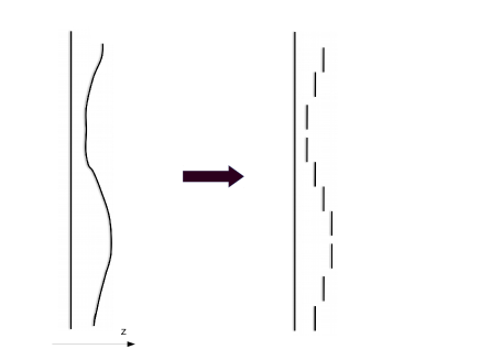
Let us see how one implements the PFA in order to calculate (from which one can extract, for instance, an approximate expression for ) expecting it to be accurate when the distance between the two surfaces is shorter than the curvature radius of the curved conductor. To that end, one first finds and approximation to the electric field between the conductors, by proceeding as follows: the smooth conductor is regarded as a set of parallel plates (Fig.1), in the sense that the electric field points along the direction and has a -independent value. The electric field does, however, depend on since it is assumed to have, for every , the same intensity as the electric field due to two (infinite) conducting planes at a distance . Namely, . Therefore, the approximated expression for the electrostatic energy becomes:
| (12) |
It is implicitly understood in the equation above, that the region to integrate is such that the assumption on the distance and curvature is satisfied. On the contrary, regions such that the assumption is not satisfied can be consistently ignored (see the example below).
It should be evident that Equation (12) provides a rather convenient tool to obtain estimates for the electrostatic energy in many relevant situations. Indeed, to illustrate this point we consider a cylinder of length and radius in front of a plane, and denote by the minimum distance between the two surfaces. The cylinder is not a surface that can be described by a single patch; namely, one needs at least two functions. However, in the context of the PFA, it is reasonably to assume that only the half that is closer to the plane should be relevant. Assuming the axis of the cylinder to be along , the function reads:
| (13) |
with the variable assumed to be in the range . Note that for the assumption on the distance and the curvature is satisfied. It is to be expected that, as long as (where the PFA gives an accurate value of the electrostatic energy), the final result will not depend on . This can be readily checked by inserting Equation (13) into Equation (12), computing the integral, and expanding that result for . Doing this we obtain:
| (14) |
which is independent of . An immediate consequence of this is that, when the cylinder approaches the plane, the electrostatic force behaves as .
Let us check now the accuracy of . We take advantage of the knowledge of the exact expression for the electrostatic interaction energy:
| (15) |
For , yields the PFA result (14). The relevance of the corrections to the PFA can be estimated by expanding the exact result, but keeping also the next-to-leading order (NTLO) when :
| (16) |
We will now introduce the DE. By construction, it should produce the NTLO result (for this an other surfaces), without resorting to the expansion of any exact expression (the knowledge of which, needless to say, is usually lacking).
III.2 Improvement of the PFA Using a Derivative Expansion
We begin by noting that the electrostatic energy is a functional of the function which defines the shape of the surface. A second observation is that, in principle, there is no reason to assume that the functional is local in . Here, “local” means that it contains just one integral over of a sum of terms involving powers of and derivatives at . On the contrary, the exact functional will generally involve terms where, for example, there are two or more integrals over , and kernels depending of those variables, and products of with different arguments. However, regardless of the non locality of the exact expression, it must become local when the surfaces are sufficiently smooth and close to each other. Indeed, if the PFA becomes valid asymptotically in that limit, then the energy must approach a result which is a local function of . Not whatever local functional but just one without derivatives.
The way we found to depart slightly but significantly from the PFA, has been to add terms involving derivatives of . Namely, we shall assume that the electrostatic energy can be expanded in local terms involving derivatives of . One can think of the condition , as introducing a small, dimensionless expansion parameter. In physical terms, this means that the curved surface is almost parallel to the plane on the points where it is satisfied.
To introduce the first departure from the PFA, we include terms with up to two derivatives. Then the electrostatic energy has to be (up to this order) of the form:
| (17) |
for some functions and . The gradient is the two-dimensional one, and it can only appear in such a way that the energy is a scalar ( is a scalar under changes of coordinates on the plane). Besides, recalling the equations of electrostatics, and on dimensional grounds, the result must be proportional to . On top of that it must reproduce for constant . Furthermore, as is the only other dimensionful quantity, both functions and have to be proportional to . Thus, we have restricted even further the functional to:
| (18) |
where is a numerical coefficient to be determined (the subindex stands for electrostatics). It is worth stressing that it is independent of the specific surface being considered, as long as it is smooth. Therefore, it can be obtained once and for all just from its evaluation for a particular case. A simple procedure to obtain the coefficient , when an exact analytic solution to the problem is known, would be to retrieve its value by expanding that solution. Let us do that for the configuration of a cylinder in front of a plane. Inserting Equation (13) into Equation (18), and performing the integrals, an expansion of the result in powers of , allow us to fix . Indeed, in order to agree with the expansion of the exact result in Equation (16), this fixes its value to . Of course, one will obtain the same value for any other particular example for which the exact solution was known.
It is worthy of noting that, since the DE is a perturbative approach, it should be desirable to have a perturbative method to calculate the coefficient . In other words, to compute it from first principles, using the appropriate expansion. One can do that, for instance, by solving perturbatively the Laplace equation and then resorting to the method described in Section V. We have performed that calculation in Ref.FLMelectro , and refer the reader to that work for details, and also for the application of the DE to other electrostatic examples.
III.3 Two Smooth Surfaces
As a natural generalization of the previously discussed situation, let us now consider two surfaces described by the two functions and , each one of them measuring the respective height of a surface with respect to a reference plane . This geometry was first considered in the context of the DE for the Casimir effect in Ref.Bimonte1 .
To construct the DE for the electrostatic energy in this case, we keep up to two derivatives of the functions. This allows we to write the general expression:
| (19) | |||||
where is the height difference, is the electrostatic energy between parallel plates, and the dots denote higher derivative terms. Equation (19) actually contains four numerical constants: , , , and . However, symmetry considerations imply some constraints on them: the energy must be invariant under the interchange of and , since that is just a relabeling: and . Furthermore, in order to reproduce the result for a single smooth surface in front of a plane we must have . The coefficient can be determined taking into account that the energy should be invariant under a simultaneous rotation of both surfaces Bimonte1 . Indeed, for an infinitesimal rotation of each surface by an angle in the plane , the changes induced on the functions are , for . To simplify the determination of we can assume that, initially, and that is only a function of . Computing explicitly the variation of to linear order in one can show that
| (20) |
and therefore
| (21) |
Note that, by taking the variation of the electrostatic energy Equation (19) with respect to translations or rotations of one of the surfaces, one can obtain the vertical and lateral components of the force, as well as the torque, due to the remaining surface.
The identities and are universally valid, regardless of the interaction (as long as the surfaces are of an identical nature), but holds true for the electrostatic interaction. This depends upon the fact that the leading term is proportional to (i.e. it is then not valid for the Casimir energy).
For later use, let us recall that, for a general function , the relation between the different coefficients becomes Bimonte1 :
| (22) |
The relation (22) shows that, for any interaction, the DE for the interaction energy between two curved surfaces can be reduced to the problem of a single surface in front of a plane. Indeed, in the later case one can determine and , while Equation (22) determines the remaining coefficient .
To summarize: when computing the electrostatic energy associated with a configuration of two conductors at different potentials, with smoothly curved surfaces, one can go beyond the PFA by simply assuming that the energy admits an expansion in derivatives of the functions that define the shapes of the conductors. If the exact electrostatic energy for a single non trivial curved configuration is known, one can determine all the free parameters in the expansion.
Finally, the NTLO correction produces an appreciable improvement in the DA and, by the same token, also provides an assessment for its validity. An interesting alternative approach to compute electrostatic forces beyond the PFA can be found in Ref. Hudlet .
IV Obtaining the DE from a Perturbative Expansion
Regardless of the interaction considered, the DA and its improvement, the DE, can be obtained by performing the proper resummation of a perturbative expansion FLMrev2014 . The required expansion is in powers of the departure of the surfaces, about a two flat parallel planes configuration. This connection yields a systematic and quite general approach to obtain the DE, even when an exact solution is not available.
To keep things general, we work with a general functional of the surface; that functional may correspond to an energy, free energy, force, etc. Besides, we do not make any assumption about the kind of interaction involved, not even about whether it satisfies a superposition principle or not.
To begin, let us we assume a geometry where there are two surfaces, one of which, , is a plane, which with a proper choice of Cartesian coordinates (, , ), is described by . The other one, , is assumed to be describable by .
The object for which we implement the approximation is denoted by , a functional of . Then we note that the PFA for , to be denoted here by , is obtained as follows: add, for each , the product of a local surface density depending only on the value of at the point , times the surface element area; namely,
| (23) |
The surface density is, in turn, determined by the (assumed) knowledge of the exact form of for the case of two parallel surfaces, as follows:
| (24) |
where denotes the area of the plate and is a constant. Namely, to determine the density one needs to know the functional just for constant functions . Note that, if the functional is the interaction energy between the surfaces, becomes the interaction energy per unit area , and becomes (see Equation (3)).
Let us now show how to derive the PFA (and its corrections) by the resummation of a perturbative expansion. To that end, we evaluate for a having the form:
| (25) |
and write the resulting perturbative expansion in powers of , which has the general form:
| (26) |
where is the Dirac delta function, and the form factors can be computed by using perturbative techniques. For the Dirichlet-Casimir effect, this can be done in a rather systematic way 4thorder . Although the approach to follow in order to obtain those form factors may depend strongly on the kind of system considered, the form of the expansion shall be the same. Note that the form factors may depend on , although, in order to simplify the notation, we will not make that dependence explicit.
Up to now, we have not used the hypothesis of smoothness of the surface. We do that now by assuming that the Fourier transform is peaked at the zero momentum. What follows is to make use of this assumption for all terms in the expansion. In Equation (26), we set then: , and, as a consequence:
| (27) |
One could evaluate the form factors at the zero momentum straighforwardly. However, there is a shortcut here that allows one to obtain all of them immediately: consider a constant , so that the interaction energy is given by Equation (27) with the replacement . For this particular case, becomes just the functional corresponding to parallel plates, which are separated by a distance :
| (28) |
We then conclude that, in this low-momentum approximation, the series can be summed up with the result:
| (29) |
which is just the PFA.
The calculation just above shows that, for the class of geometries considered in this paper, the PFA can be justified from first principles as the result of a resummation of a perturbative calculation corresponding to almost flat surfaces. In order to be well defined, the PFA requires that the form factors have a finite limit as .
This procedure also suggests how the PFA could be improved; one can include the NTLO terms in the low-momentum expansions of the form factors. We assume that they can be expanded in powers of the momenta up to the second order. We stress that this is by no means a trivial assumption. Indeed, depending on the the interaction considered, the form factors could include nonanalyticities (we will discuss some explicit examples below). In case of no nonanalyticities, one can introduce the expansions:
| (30) |
for some dependent coefficients and . Here label arguments while label their components. Symmetry considerations are crucial, since they allow us to simplify the above expression (30), as follows: rotational invariance implies that the form factors depend only on the scalar products . Additionally, they have to be symmetric under the interchange of any two momenta. This thus leads to
| (31) |
for some coefficients and .
Inserting Equation (31) into Equation (26) and taking integrations by parts, one then finds the form of the first correction to the PFA:
| (32) |
where the coefficients are linear combinations of and . The subindex in indicates that this is the part of the functional containing two derivatives.
We complete the calculation by calculating the sum in Equation (32). To that end, we evaluate the correction for a particular case: , with , and expand up to the second order in . Thus,
| (33) |
The resummation can be obtained in this case, by considering the usual perturbative evaluation of the interaction energy up to second order in . This evaluation does, naturally, depend on the interaction considered, but, once one has that result one can obtain the sum of the series above. We we will denote by that sum, namely:
| (34) |
Upon replacement in Equation (34), one obtains
| (35) |
This is the NTLO correction to the PFA. This concludes our systematic derivation of the PFA, including its first correction, a result which may be put as follows:
| (36) |
where is determined from the (known) expression for the interaction energy between parallel surfaces, while can be computed using a perturbative technique. In practice, can be evaluated setting in Equation (34).
The higher orders may be derived by an extension of the procedure described just above. It should be evident that, for the expansion to be well-defined, the analytic structure of the form factors is quite relevant. Indeed, the existence of nonanalytic zero-momentum contributions can render the DE non applicable. This should be expected on physical grounds, since the presence of nonanalytic terms implies that the functional cannot be approximated, in coordinate space, by the single integral of a local density. Physically, it is a signal that the nonlocal aspects of the interaction cannot be ignored. That should not come up as a surprise, when one recalls that the same kind of phenomenon does happen when evaluating the effective action in quantum field theory, and the quantum effects contain contributions due to virtual massless particles. In this case, the effective action may develop nonanalyticities at zero momentum.
The main messages of this Section are the following: irrespective of the nature of the interaction, the energy and forces between objects are functionals of their shapes. The PFA is recovered when the form factors of the functionals are evaluated at zero momentum. Enhancements to this approximation are achievable by expanding these form factors at low momenta. If the expansion is analytic, a resummation of the form factors produces the DE.
V DE for the Zero-Temperature Casimir Effect
The application of the DE to the Casimir interaction energy between two objects was, actually, our original motivation to introduce the approximation, and it is useful briefly review some aspects of this application here. We consider first a real vacuum scalar field satisfying Dirichlet boundary conditions (Section V.1) and then we move to the EM field with perfect-conductor boundary conditions (Section V.2). We follow Ref. FLM2011 for the derivation of the DE in the Dirichlet case.
V.1 Scalar Field with Dirichlet Boundary Conditions
We consider here a massless real scalar field in dimensions, coupled to two mirrors which impose Dirichlet boundary conditions. In our Euclidean conventions, we use to denote the spacetime coordinates, being the imaginary time. As before, the mirrors occupy two surfaces, denoted by and , defined by the equations and , respectively.
On only dimensional grounds, and using natural units (), the DE approximation to the interaction energy to be of the form
| (37) |
where and are dimensionless coefficients that do not depend on the geometry. The subindex stands for Dirichlet. An evaluation of the above expression for parallel plates fixes . As in the electrostatic case, the coefficient could be computed from explicit examples where the interaction energy is known exactly.
Let us recall, from Section IV, that the interaction energy can also be computed from an expansion of the Casimir energy in powers of for
| (38) |
where (assumed to be greater than zero) is the spatial average of whereas contains its varying piece. The expansion needed is of the second order in , and with up to two spatial derivatives.
To obtain such an expansion, we start from a rather general yet formal expression for the energy (for earlier perturbative computations of the Casimir force see, for example, Ref.earlier-pert1 ; earlier-pert2 ). That formal expression follows from the functional approach to the Casimir effect, where we deal with , the zero-temperature limit of a partition function. That partition function, for a scalar field in the presence of two Dirichlet mirrors is given by
| (39) |
with denoting the real scalar field free (Euclidean) action
| (40) |
while the and impose Dirichlet boundary conditions on the and surface, respectively.
The vacuum energy, , is then obtained as follows:
| (41) |
where is the extent of the time dimension (or , in a thermal partition function setting). We discard from the terms that do not contribute to the Casimir interaction energy between the two surfaces. These terms will appear as factors in ; among them the one describing the zero point energy of the field in the absence of the plates, and also the ‘self-energy’ contributions, due to the vacuum distortion produced by each mirror, even when the other is infinitely far apart.
Exponentiating the two Dirac delta functions by introducing two auxiliary fields, and , we obtain for an equivalent expression:
| (42) |
with
where we have introduced . The factor depending on the determinant of the induced metric on the , makes the expression above reparametrization invariant. However, by a redefinition of the auxiliary field one gets rid of that factor, at the expense of generating a Jacobian. That Jacobian does not depend on the distance between the two surfaces, since only derivatives of are involved. Therefore it will not contribute the the Casimir interaction energy and thus we shall subsequently ignore such factor, as well as others that will appear in the course of the calculations.
Integrating out , we see that , corresponding to the field in the absence of boundary conditions factors out, while the rest becomes an integral over the auxiliary fields:
| (43) |
with:
| (44) |
and . We have introduced the objects:
| (45) | ||||
| (46) | ||||
| (47) | ||||
| (48) |
where we use a “bra-ket” notation to denote matrix elements of operators, and is the four-dimensional Laplacian. Thus, for example,
| (49) |
A subtraction of the zero point contribution contained in leads to:
| (50) |
which still contains self-energies. Up to now, we have obtained a formal expression for the vacuum energy; let us now proceed to evaluate its DE.
We need to expand to the second order in , keeping up to the second order term in an expansion in derivatives. It is convenient to do so first for . Namely,
| (51) |
where the upper index denotes the order in derivatives. Each term will be a certain coefficient times the spatial integral over of a local term, depending on and on -derivatives. Additionally, because the configuration is time-independent, they should be proportional to (a factor that will cancel out). Expanding first the matrix in powers of
| (52) |
we obtain: ,
| (53) | |||||
where, in , we need to keep up to derivatives of .
Then, the zeroth-order term is obtained as follows: replace by a constant, , and then subtract from the result its limit (this gets rid of self-energies). This leads to:
| (54) |
Here, the are identical to the ones for two flat parallel mirrors separated by a distance .
Taking the trace, leads to:
| (55) |
Then, we recall the general derivation to note that the replacement leads to:
| (56) | |||||
which is the PFA expression for the vacuum energy.
To improve on the previous result, we consider its first non trivial correction. There can be no first order term because of symmetry considerations. while to terms contribute to the second order
| (57) |
where,
| (58) |
and
| (59) |
In the terms above, we have to keep just up to two derivatives of . We see that, in Fourier space, and before implementing any expansion in momentum (derivatives), they have the structure:
| (60) |
(), with denoting the Fourier transform of , and with the kernels denoting the (i.e., static) limits of the more general expressions:
By subtracting all the -independent contributions, one finds:
| (61) |
with:
| (62) |
The low-momentum behaviour of determines whether the DE can be applied or not. In this case, the function is analytic and therefore a local expansion of the vacuum energy exists. We need to extract its order term in a Taylor expansion at zero momentum, namely . We find:
| (63) |
Thus,
| (64) | |||||
Therefore, the NTLO term in the DE becomes:
| (65) |
where the index runs from to .
Putting together the terms up to second order,
| (66) |
The leading-order term above is the Casimir energy according to the PFA , while the second order one represents the first significant deviation from it. We note that the structure of both terms had been anticipated by dimensional analysis and symmetry considerations. The overall normalization, on the other hand, had been fixed by our previous knowledge of the (well-established) result for parallel plates.
We would like to insist on the fact that the relative weight between the PFA and its correction term–the factor –is independent of the surface geometry. This value of has been independently corroborated in concrete examples by expanding the exact Casimir energy expressions. Interesting cases among them are, for example, either a sphere or a cylinder positioned in front of a plane.
We conclude this Section with an application of the DE to the particular geometry of a sphere in front of a plane. Let us express the function of Equation (13) in polar coordinates , with the radius of the sphere and the distance to the plane. The function describes an hemisphere when . By inserting the expression of into the DE for the Casimir energy, it becomes possible to explicitly calculate the integrals, to get a rather compact analytical expression:
| (67) |
where .
V.2 The EM Case
The results for the scalar field satisfying Dirichlet boundary conditions, described in Section (V.1) above, have been generalized to different boundary conditions and fields. Results for the EM field case and two curved surfaces have been presented in Ref.Bimonte1 . Note that, as pointed out at the end of Section III.3, symmetry considerations allow for the two-surface problem to be reduced to the one of a curved surface facing a plane, namely, the geometry we have just dealt with in the Dirichlet case above. Indeed, as shown in Ref. Bimonte1 , the extension of Ref.FLM2011 to two curved surfaces is restricted among other things by the tilt invariance of the reference plane, to which the two surfaces can be projected. This served as a rigorous test for the self-consistency of perturbative results.
Venturing beyond the scalar Dirichlet (D) case of Ref.FLM2011 , they calculated the DE for Neumann (N), mixed D/N, and electromagnetic (EM) (perfect metal) surfaces. Interestingly, they observed that the EM correction must align with the sum of D and N corrections. They also replicated previous findings for cylinders under D, N, and mixed D/N conditions, as well as for the sphere with D boundary conditions. However, their calculations did not confirm previous results for the sphere/plane geometry, either with N or EM boundary conditions. Indeed, the results for were found to disagree with those obtained from Refs. bordag08 ; bordag101 ; bordag102 . This discrepancy was later resolved in Ref.bordag-teo in favour of the results in Bimonte1 .
Another interesting concrete example presented in Bimonte1 is the DE for two spheres of radii and , both imposing the same boundary conditions. It was found there that
| (68) |
where ; is chosen to be the distance of closest separation, and is a number that depends on the type of boundary condition, as can be seen from Table 1. in the EM boundary conditions case. The corresponding formula for the sphere/plane case can be obtained by taking one of the two radii to infinity (in fact it coincides with the D case in Equation (67) when and ).
A rather different example corresponds to two circular cylinders (with identical boundary conditions) whose axes are inclined at a relative angle . Using the DE, the interaction Casimir energy reads:
| (69) |
For this particular geometry, the interaction energy has been computed numerically in Rodriguez . The numerical results reproduce Equation (69) at short distances.
The results obtained for the -coefficients in each case are summarized in Table 1.
| 2/3 | 2/3 |
Having presented in this Section a derivation and some interesting results obtained by applying the DE to the Casimir effect at zero temperature and for perfect boundary conditions, we present in the rest of the review some generalizations and applications.
VI Finite Temperature, Nonanalyticities, and DE
The DE can be extended to the finite temperature case Bimonte2 ; FLMTdim ; FLMTem , the free energy being the relevant functional to approximate. There are at least two reasons why this extension is not trivial: firstly, the temperature introduces a dimensionful magnitude, and this will reflect itself in the form of the DE (part of it was fixed by dimensional analysis). Second, a known phenomenon in quantum field theory at finite temperature is the so-called ”dimensional reduction”, by which a bosonic model which is defined in dimensions at zero temperature, becomes effectively -dimensional at high temperatures. The DE should therefore manifest (and interpolate between) those two cases.
We first describe, in Section VI.1, the results for a scalar field satisfying Dirichlet conditions FLMTdim in dimensions. Then, Section VI.2 discusses the appearance of nonanaliticities for Neumann boundary conditions FLMTdim ; FLMNeu . Finally, we comment on the results for the EM field with imperfect boundary conditions FLMTem ; Bimonte2 (Section VI.3) and on semianalytic formula for plane–sphere geometry (Section VI.4).
VI.1 Dirichlet Boundary Conditions
In the finite-temperature case, and for the same geometry that we have considered in the zero temperature case, the functions and cannot be completely determined from dimensional analysis alone. Indeed, on general grounds, we can assert that the Casimir free energy in dimensions, if the DE is applicable, must have the form:
| (70) |
where and are dimensionless and depends on the ratio of the local distance between surfaces and the inverse temperature . They can be obtained from the knowledge of the Casimir free energy for small departures around . They are given by FLMTdim
| (71) |
where
| (72) |
In the zero temperature limit, the Matsubara sum becomes an integral that can be analytically computed. The results are described in Table 2. The ratio tends to for large values of .
| Dimension | Approximate Value | |
|---|---|---|
In the high temperature limit, we find
| (73) | |||||
where . The coefficients and agree with those for perfect mirrors at zero temperature, but in dimensions, i.e., the ‘ dimensional reduction” effect.
An interesting result is found when this is applied to the (Dirichlet) Casimir interaction for a system consisting of a sphere in front of an infinite plane. Denoting by the distance between the surfaces, and by the radius of the sphere, we get for the free energy at high temperatures:
| (74) |
We see that the -behavior corresponding to the dominant contribution at zero temperature changes to in the high temperature case. This could be expected on dimensional grounds, if one assumes that the free energy is linear in the temperature in this limit. Note that the same problem has been exactly solved in Ref.bimonteprl , and one can show that Equation (74) does agree with the small-distance expansion obtained from the exact solution.
It is worth to remark that the NTLO correction from the DE becomes nonanalytic, because of the integration, in the ratio . This behavior has been observed in numerical calculations of the Casimir interaction energy for this geometry, in the infinite temperature limit, for the electromagnetic case (see Refs.bimonteprl ; Neto2012 ). It is important to recognize that this nonanalyticity has nothing to do with the nonanalyticity in momenta of the form factors described in Section 4, and is a non trivial prediction of the DE.
VI.2 Neumann Boundary Conditions
This case, discussed in Ref.FLMNeu , highlights a potential warning to the applicability of the DE, already mentioned previously: the appearance of nonanalyticities in the form factors. To begin with, we deal with the zero temperature case in dimensions, since the nonanalyticity appears because of the existence of a Matsubara mode which behaves as a massless field in dimensions, with Neumann boundary conditions.
The free Euclidean action for the vacuum (i.e., ) field is given by
| (75) |
and, instead of imposing perfect Neumann boundary conditions on the surfaces, we add the following action to describe the interaction between the vacuum field and the mirrors:
| (76) |
The constant , which has the dimensions of a mass, is used to impose Neumann boundary conditions in the limit. We use the same on both L and R mirrors, since we will assume them to have identical properties, differing just in their position and geometry.
The DE approximation to the Casimir energy can be computed following standard steps. The result reads, in the limit FLMNeu ,
| (77) |
In the expression above, the first term is the PFA contribution while the second one is a non trivial correction to it, and depends on the shape of the boundary (defined by ). It is then clear that, as this equation shows, the DE is well posed when imposing imperfect Neumann boundary conditions in dimensions. On the contrary, it cannot be applied when the boundary conditions become perfect (). The reason is that the hypothesis of analyticity in momentum, used to derive the DE, is clearly violated. The non-existence of a local expansion is due to the existence of massless modes, allowed by Neumann boundary conditions.
Since, at finite temperatures, a dimensional theory may be decomposed into the sum of an infinite tower of decoupled dimensional Matsubara modes, each one satisfying N boundary conditions, and with a mass , The existence of the massless mode (the only one surviving in the high temperature limit) means that analyticity will be lost in dimensions, for any non zero temperature. That is indeed the case FLMTdim . We summarize here some of the main features of that example: the free energy in the dimensional Neumann case can again be written as before (see Eq.(70), but with coefficients and instead of and . The zero order term coincides with the one for the Dirichlet case; namely: .
When , the NTLO term contains, besides a local term, a nonlocal contribution which is linear in , and thus present for any . Hence, there is no local DE for perfect Neumann boundary conditions at at zero temperature and for at any finite temperature. Indeed, an expansion for small values of of the form factor contains, in addition to a term proportional to , one proportional to .
VI.3 The Electromagnetic Case for Imperfect Boundary Conditions
We have seen that, for a real scalar field in the presence of Neumann boundary conditions, the DE cannot be applied when in dimensions at zero temperature, or in dimensions at a non-zero temperature FLMTdim . The reason is that, as we have shown, nonanalyticities in the form factors appear. We have shown that the nonanalyticity could be cured by introducing a small departure from perfect Neumann conditions FLMNeu . It is natural to wonder whether the nonanalyticities could also be cured by a similar approach for the EM field in dimensions at finite temperatures. We know, based on the insight obtained from Ref.FLMNeu , that nonanalyticities are originated in contributions due to dimensionally reduced massless modes: zero Matsubara frequency terms. To obtain an answer to this question, in Ref.FLMTem we singled out in detail the zero-mode contributions to the free energy, for a media described by non trivial permittivity and permeability functions.
We start from the free energy for the EM field, which can be written in terms of the partition function , as follows:
| (78) |
where the denominator, , denotes the partition function for the EM field in the absence of media and
| (79) |
The gauge invariant action reads
| (80) |
Here, indices like run over spatial indices, Einstein summation convention is assumed, and and denote the imaginary time versions of the permittivity and permeability, respectively ( is the inverse integral kernel of ).
The geometry of the system is determined by same two surfaces and we have considered before, and defined by and , but now they correspond to the boundaries of the media, i.e.,
where and characterize the permittivity and permeability of the respective mirror.
We can expand the fields and the electromagnetic properties as
| (81) |
where () are the Matsubara frequencies.
Inserting these expansions into the partition function one can readily check the factorization
| (82) |
and therefore
| (83) |
As mentioned, we are particularly interested in the contribution,
| (84) |
where
| (85) |
and
| (86) |
Note that vanishes for a dielectric and also for a metal described by the Drude model. On the other hand, it equals the plasma frequency for a metal described by the plasma model.
The zero mode contribution to the free energy therefore splits into a scalar () and a vector () contribution, the former associated to the field and the later to
| (87) |
To discuss the emergence of non-analyticities in the derivative expansion we computed and assuming up to second order in . The quadratic contributions can be written as
| (88) |
and the crucial point is whether the functions are analytic or not in .
Omitting the details, we summarize the main results FLMTem : for finite values of and , the scalar contribution analytic, including the limit , in which it tends to the dimensional Dirichlet value. It develops a nonanalytic (logarithmic) contribution for , since the kernel corresponds in this case to that of a scalar field in dimensions satisfying Neumann boundary conditions. In other words, magnetic materials regulate the non-analyticity of the TE zero mode.
On the other hand, the TM zero mode is nonanalytic whenever as for both mirrors. In terms of the models usually considered in the Casimir literature to describe real materials, this condition corresponds to the plasma model.
VI.4 A Semianalytic Formula for Plane-Sphere Geometry
As a final application of the DE to compute the Casimir free energy we mention the results of Ref.Bimonte3 , where the author combined exact calculations for the zero mode and the DE to obtain a precise formula for the interaction between a sphere and a plane at a finite temperature which is valid at all separations. We briefly describe here these findings.
Formally, the free energy for this geometry can be written as
| (89) |
where the sum is over the Matsubara frequencies and denotes scattering matrix elements for this geometry. The prime on the sum indicates that the term has an additional factor.
The contribution can be computed exactly using the Drude model to describe the materials of the plane and the sphere, and plays a crucial role. Indeed, the proposed approximation for the Casimir force on the sphere of radius at a distance from the plane is
| (90) |
where can be computed using the DE. Notably, describes with high precision the Casimir force at all separations, as can be checked by comparison with high precision numerical simulations of the exact scattering formula.
These results have been generalized in subsequent studies to the case of the two spheres- geometry Bimonte4 , also considering the differences that come from the use of the Drude vs plasma models, as well as for grounded vs isolated spheres Bimonte5 . The relevance of the use of grounded conductors in Casimir experiments has also been discussed in Ref. FLMgrounded .
VII Casimir-Polder Forces
The DE approach has also been applied to the calculation of the Casimir-Polder interaction between a polarizable particle and a gently curved surface BimonteCP . We present in this Section a simplified version of the results contained in that reference.
When a small polarizable particle is at a distance of a planar surface, the Casimir-Polder potential reads Bordagbook
| (91) |
where is the frequency dependent polarizability (which is assumed isotropic), , and
| (92) |
For moderate distances such that one obtains the usual Casimir-Polder potential Casimir-Polder
| (93) |
Assume now that the particle is in front of a slightly curved surface. The particle is at the origin of coordinates, and the surface is described, as usual, by the height function . The DE for the Casimir-Polder interaction assumes that the interaction depends on the derivatives of the height function evaluated at , the point on the surface closest to the particle (a local minimum for ). If the surface is homogeneous and isotropic, then the interaction energy must be invariant under rotations of the coordinates. The more general expression compatible with this properties describes the Casimir -Polder interaction energy at reads BimonteCP :
| (94) |
The dimensionless function can be read from the perturbative expansion of the potential , carried to second order in the deformation, that is, for with . We stress that here the Casimir-Polder energy is not a functional but a function of and its derivatives evaluated at the origin of coordinates (recall that ). The DE is expected to be valid when , the radii of curvature of the surface at . Note that and
| (95) |
Using again the static polarizability approximation, , one obtains
| (96) |
The results presented in Ref. BimonteCP are much more general than those described here: they include the Casimir-Polder potential for a general polarization tensor and higher order corrections proportional to , as well as the details of the computation of the corresponding functions . Additional applications can be found in moreCP1 ; moreCP2 .
VIII Other Techniques Beyond PFA
In Ref. pauloEPL a detailed analysis of the Casimir effect’s roughness correction in a setting involving parallel metallic plates is presented. The plates were defined through the plasma model. The approach used is perturbative, factoring in the roughness amplitude and allowing for the consideration of diverse values of the plasma wavelength, plate separation, and roughness correlation length. A notable finding was that the roughness correction exceed the predictions of the PFA. The authors have calculated the second-order response function, , across a spectrum of values encompassing the plasma wavelength (), distance (), and roughness wave vector ():
| (97) |
applicable when . Here, represents the plate surface area, the dimensionless integration variable denoting the imaginary wave vector’s -component scaled by plate separation , the longitudinal component of the imaginary wave vector for the diffracted wave, and .
The calculation in Ref. pauloEPL helps to compute the second-order roughness correction as a function of the surface profiles, and . Analytical solutions were determined for specific limiting cases, revealing a more complex relationship with the perfect reflectors model than previously recognized pauloEPL03 ; emigPRL01 , particularly in scenarios involving extended distances and small roughness wavelengths. While the asymptotic case of long roughness wavelengths aligns with PFA predictions, it was established that PFA generally underestimates the roughness correction, a critical aspect for exploring constraints on potentially new weak forces at sub-millimeter ranges.
As a further expansion to pauloEPL , in Ref. pauloUniverse21 , the authors explored the Casimir interaction between a plane and a sphere of radius at a finite temperature , in terms of the distance of closest approach, . Noting that, under the usual experimental conditions, the thermal wavelength satisfies , they evaluated the leading correction to the PFA, applicable to such intermediate temperatures. They resorted to developing the scattering formula in the plane-wave basis. The result captures the combined effect of spherical geometry and temperature, and is expressed as a sum of temperature-dependent logarithmic terms. Remarkably, two of these logarithmic terms originated from the Matsubara zero-frequency contribution.
Defining the variables and , and the deviation , in the intermediate temperature regime , it is found in Ref. pauloUniverse21 that
| (98) |
The leading neglected terms stem from non-zero Matsubara frequencies.
In Ref. pauloOSA , the leading-order correction to PFA in a plane-sphere geometry was derived. The momentum representation connected this with geometrical optics and semiclassical Mie scattering. The primary contributions are shown to come from diffraction, with TE polarization becoming more relevant than TM polarization. The diffraction contribution is calculated at leading order, using the saddle-point approximation, considering leading order curvature effects at the sphere tangent plane.
Additionally, the next-to-leading order (NTLO) term in the saddle-point expansion contributed to the PFA correction. This involved computing the round-trip operator within the WKB approximation, representing sequences of reflections between the plane and the sphere. A key aspect was the tilt in the scattering planes, allowing TE and TM polarizations to mix.
Comprehending the implications of polarization mixing channels on the geometric optical correction applied to PFA holds considerable importance. Indeed, these channels are recognized for inducing negative Casimir entropies with a geometric foundation. 24–26OSA1; 24-26OSA2 ; 24-26OSA3 ; 49-51OSA1 ; 49-51OSA2 ; 49-51OSA3 . In spite of the non-vanishing contribution of the polarization mixing matrix elements, the total correction associated with the tilt between the scattering and Fresnel planes is zero at NTLO. This implies that the primary correction to the PFA would remain unchanged even if the complexities arising from the differences between the Fresnel and scattering polarization bases were initially ignored. The latter points to the fact that a different approach, one that completely omits the effect of polarization mixing, could directly produce the leading order correction to PFA. Plane waves proved to be a well-suited basis for studying the Casimir effect, as has been evidenced in the more recent study paulo22 . The utility of that basis ranges from analytical to numerical applications, particularly when dealing with objects in close proximity, the most relevant situation in experiments. It has been also shown that the use of plane waves was notably effective in improving the interpretation of results in the realms of geometrical optics and diffractive corrections.
In the context of a setup involving two spheres with arbitrary radii in vacuum, it was shown in paulo22 that the PFA emerged as the leading term in an asymptotic expansion for large radii. Extending a prior calculation based on the saddle-point approximation, involving a trace over multiple round-trips of electromagnetic waves between the spheres, the study encompassed spheres made of bi-isotropic material, requiring the consideration of polarization mixing during reflection processes. The result was naturally elucidated within the framework of geometrical optics.
Then, by relying on a saddle-point approximation framework, the authors derived leading-order corrections, of geometrical and diffractive origins. Explicit results, at first obtained for perfect electromagnetic conductors (PEMC) spheres at zero temperature, indicated that for certain material parameters, the PFA contribution vanishes; should that be the case, the leading-order correction would be the dominant term in the Casimir energy.
In the lowest-order saddle-point approximation, but including diffractive corrections, one can show that the expression for the Casimir energy becomes:
| (99) |
where . As expected, this result reproduces the PFA result and its leading-order diffractive correction. The NTLO correction behaves as . However, the prefactor obtained accounts for about of the one coming from numerical results pauloOSA . This discrepancy may be traced back to having neglected the NTLO-SPA and NNTLO-SPA contributions.
IX Conclusions
In this review, we have discussed several properties and applications of the DE approach, mostly as a method to improve the predictions of the Proximity Force Approximation, of long standing use in many different fields.
We started the review by briefly discussing the precursor of the PFA: the Derjaguin (and related) approximations, since we have found them rather appropriate in order to display the essentially geometric nature of the kind of problem we discuss: two quite close smooth surfaces, and an interaction energy between them. Depending on the kind of system being considered, that interaction between the two surfaces may or not be the result of the superposition of the interactions between pairs. An example of an interaction which is not the result of such a superposition is the Casimir effect. Note, however, that even when the fundamental interaction satisfies a superposition principle, like in electrostatics, the actual evaluation of the Coulomb integral to calculate the total interaction energy could be a rather involved problem because the actual charge density may not be known a priori. That is indeed the case when the surfaces involved are conductors, since that usually requires finding the electrostatic potential. We have used precisely this problem in order to present the idea of the DE in a concrete example: to calculate the electrostatic energy between two conducting surfaces held at different potentials.
After introducing and applying the DE in that example, we have discussed its more general proof of that expansion, by first putting the problem in a more general and abstract way: how to approximate, under certain smoothness assumptions, a functional of a pair of surfaces. At the same time, the proof provides a concrete way to determine the PFA and its NTLO correction, the DE: one just needs to perform an expansion in powers of the deformation of the surfaces about the situation of two flat and parallel surfaces.
The derivations and examples here have been presented for a geometrical setting were one surface is a plane, while the other may be described by a single Monge patch based on that plane. However, as shown by other authors, under quite reasonable and general assumptions, the results obtained for that situation may be generalized to the case of two curved surfaces parametrized by their respective patches, based on a common plane (which now does not coincide with one of the physical surfaces).
Then we reviewed different applications of the DE to the zero temperature Casimir effect, considering different fields and boundary conditions, staring from the cases of the scalar field with Dirichlet boundary conditions, then the EM field in the presence of perfectly conducting surfaces, and commented on the scalar field with Neumann conditions.
We afterwards presented a description and brief review of the extension of DE to finite temperature cases, and different numbers of spatial dimensions. The temperature is a dimensionful magnitude and the phenomenon of dimensional reduction presents a problem when there are Neumann boundary conditions or when an EM field is involved. Indeed, dimensional reduction implies the existence of a massless dimensional field (with Neumann conditions), and this mode introduces a nonanalyticity in momentum space, which violated one of the hypothesis of the DE, and therefore it cannot be applied. Nevertheless, we have shown that the introduction of a small departure from ideal Neumann conditions solves this issue, namely, analyticity is recovered and the DE may be applied.
We also mentioned the application of DE to the Casimir-Polder interaction, particularly between a polarizable particle and a gently curved surface. This example highlights the broader implications of DE in understanding particle-surface interactions beyond the Casimir force itself.
To conclude, we have presented in this review the main features of the DE approach, with a focus in the Casimir effect, but pointing at the fact that its applicability can certainly go beyond that realm. We have shown that explicitly for electrostatics, but we expect it to be applicable to, for example, the same kind of systems where the DA, SEI and SIA were introduced.
This research was funded by Agencia Nacional de Promoción Científica y Tecnológica (ANPCyT), Consejo Nacional de Investigaciones Científicas y Técnicas (CONICET), Universidad de Buenos Aires (UBA), and Universidad Nacional de Cuyo (UNCuyo), Argentina.
References
- (1) Casimir, H.B.G. On the attraction between two perfectly conducting plates. Proc. Kon. Ned. Akad. Wetensch. B 1948, 51, 793 – 795. Available online: https://dwc.knaw.nl/DL/publications/PU00018547.pdf (accessed on 6 Januaary 2023).
- (2) Milonni, P.W. The Quantum Vacuum. An Introduction to Quantum Electrodynamics; Academic Press, Inc.: San Diego, CA, USA, 1994. https://doi.org/10.1016/C2009-0-21295-5
- (3) Milton, K.A. The Casimir Effect. Physical Manifestations of Zero-Point Energy; World Scientific: Singapore, 2001. https://doi.org/10.1142/4505
- (4) Bordag, M.; Klimchitskaya, G.L.; Mohideen, U.; Mostepanenko, V.M. Advances in the Casimir Effect; Oxford University Press: Oxford, UK, 2009. https://doi.org/10.1093/acprof:oso/9780199238743.001.0001
- (5) Dalvit, D.; Milonni, P.; Roberts, D.; da Rosa, F. (Eds.) Casimir Physics; Springer: Berlin/Heidelberg, Germany, 2011. https://doi.org/10.1007/978-3-642-20288-9
- (6) Mostepanenko, V.M. Casimir puzzle and Casimir conundrum: Discovery and search for resolution. Universe 2021, 7, 84.
- (7) Bressi, G.; Carugno, G.; Onofrio, R.; Ruoso, G. Measurement of the Casimir force between parallel metallic surfaces. Phys. Rev. Lett. 2002, 88, 041804.
- (8) Brown-Hayes, M.; Dalvit, D.A.R.; Mazzitelli, F.D.; Kim, W.J.; Onofrio, R. Towards a precision measurement of the Casimir force in a cylinder-plane geometry. Phys. Rev. A 2005, 72, 052102.
- (9) Lamoreaux, S.K. Demonstration of the Casimir force in the 0.6 to 6 m range. Phys. Rev. Lett. 1997, 78, 5–8.
- (10) Mohideen, U.; Roy, A. Precision measurement of the Casimir force from 0.1 to 0.9 m. Phys. Rev. Lett. 1998, 81, 4549–4552.
- (11) Chan, H.B. Aksyuk, V.A. Kleiman, R.N. Bishop, D.J. Capasso, F. Quantum mechanical actuation of microelectromechanical system by the Casimir effect. Science 2001, 291, 1941–1944.
- (12) Decca, R.S.; López, D.; Fischbach, E.; Klimchitskaya, G.L.; Krause, D.E.; Mostepanenko, V.M. Precise comparison of theory and new experiment for the Casimir force leads to stronger constraints on thermal quantum effects and long-range interactions. Ann. Phys. 2005, 318, 37–80.
- (13) Chang, C.C.; Banishev, A.A.; Castillo-Garza, R.; Klimchitskaya, G.L.; Mostepanenko, V.M.; Mohideen, U. Gradient of the Casimir force between Au surfaces of a sphere and a plate measured using an atomic force microscope in a frequency-shift technique. Phys. Rev. B 2012, 85, 165443.
- (14) Bimonte, G.; López, D.; Decca, R.S. Isoelectronic determination of the thermal Casimir force. Phys. Rev. B 2016, 93, 184434.
- (15) Bimonte, G.; Spreng, B.; Maia Neto, P.A.; Ingold, G.-L.; Klimchitskaya, G.L.; Mostepanenko, V.M.; Decca, R.S. Measurement of the Casimir force between 0.2 and 8 : Experimental procedures and comparison with theory. Universe 2021, 7, 93.
- (16) Boyer, T.H. Quantum electromagnetic zero point energy of a conducting spherical shell and the Casimir model for a charged particle. Phys. Rev. 1968, 174, 1764–1774.
- (17) Derjaguin, B.V. Untersuchungen über die Reibung und Adhäsion, IV. Koll.-Z. 1934, 69, 155–164. https://doi.org/10.1007/BF01433225
- (18) Deriagin, B.V.; Abrikosova, I.I. Direct measurement of the molecular attraction of solid bodies. I. Statement of the problem and method of measuring forces by using negative feedback. Sov. Phys. JETP 1957, 4, 819–829. Available online: http://jetp.ras.ru/cgi-bin/e/index/e/3/6/p819?a=list (Accessed on 6 January 2024).
- (19) Derjaguin, B.V. The force between molecules. Sci. Am. 1960, 203, 47. htts://doi.org/10.1038/scientificamerican0760-47
- (20) Israelachvili, J.N. Intermolecular and Surface Forces; Academic Press Elsevier, Inc.: Oxford, UK, 2011. https://doi.org/10.1016/C2009-0-21560-1
- (21) Fosco, C.D.; Lombardo, F.C.; Mazzitelli, F.D. The proximity force approximation for the Casimir energy as a derivative expansion. Phys. Rev. D 2011, 84, 105031.
- (22) Fosco, C.D.; Lombardo, F.C.; Mazzitelli, F.D. An improved proximity force approximation for electrostatics. Ann. Phys. 2012, 327, 2050–2059.
- (23) Fosco, C.D.; Lombardo, F.C.; Mazzitelli, F.D. Derivative-expansion approach to the interaction between close surfaces. Phys. Rev. A 2014, 89, 062120.
- (24) Bimonte, G.; Emig, T.; Jaffe, R.; Kardar, M. Casimir forces beyond the proximity approximation. Europhys. Lett. 2012, 97, 50001.
- (25) Bimonte, G.; Emig, T.; Kardar, M. Material dependence of Casimir forces: Gradient expansion beyond proximity. App. Phys. Lett. 2012, 100, 074110.
- (26) Fosco, C.D.; Lombardo, F.C.; Mazzitelli, F.D. Derivative expansion for the Casimir effect at zero and finite temperature in dimensions. Phys. Rev. D 2012, 86, 045021.
- (27) Fosco, C.D.; Lombardo, F.C.; Mazzitelli, F.D. Derivative expansion for the electromagnetic and Neumann Casimir effects in dimensions with imperfect mirrors. Phys. Rev. D 2015, 91, 105019.
- (28) Fosco, C.D.; Lombardo, F.C.; Mazzitelli, F.D. On the derivative expansion for the electromagnetic Casimir free energy at high temperatures. Phys. Rev. D 2015, 92, 125007.
- (29) Bimonte, G.; Emig, T.; Kardar, M. Casimir-Polder interaction for gently curved surfaces. Phys. Rev. D 2014, 90, 081702.
- (30) Schoger, T.; Spreng, B.; Ingold, G.L.; Neto, P.A.M. Casimir effect between spherical objects: Proximity-force approximation and beyond using plane waves. Int. J. Mod. Phys. A 2022, 37, 2241009.
- (31) Blocki, J.; Randrup, J.; Swiatecki, W.J.; Tsang, C.F. Proximity forces. Ann. Phys. 1977, 105, 427–462.
- (32) Blocki, J.; Swiatecki, W.J. A generalization of the proximity force theorem. Ann. Phys. 1981, 132, 53–65.
- (33) Myers, W.D.; Swiatecki, W.J. Nucleus-nucleus proximity potential and superheavy nuclei. Phys. Rev. C 2000, 62, 044610.
- (34) Dutt, I.; Puri, R.K. Comparison of different proximity potentials for asymmetric colliding nuclei. Phys. Rev. C 2010, 81, 064609.
- (35) Bhattacharjee, S.; Elimelech, M. Surface element integration: A novel technique for evaluation of DLVO interaction between a particle and a flat plate. J. Colloid. Interface Sci. 1997, 193, 273–285.
- (36) Dantchev, D.; Valchev, G. Surface integration approach: A new technique for evaluating geometry dependent forces between objects of various geometry and a plate. J. Colloid Interface Sci. 2012, 372, 148–163.
- (37) Decca, R.S.; Fischbach, E.; Klimchitskaya, G.L.; Krause, D.E.; Lopez, D.; Mostepanenko, V.M. Application of the proximity force approximation to gravitational and Yukawa-type forces. Phys. Rev. D 2009, 79, 124021.
- (38) Milton, K.A.; Parashar, P.; Wagner, J.; Shajesh, K.V. Exact Casimir energies at nonzero temperature: Validity of proximity force approximation and interaction of semitransparent spheres. arXiv 2009, arXiv:0909.0977. https://doi.org/10.48550/arXiv.0909.097
- (39) Hudlet, S.; Saint Jean, M.; Guthmann, C.; Berger, J. Evaluation of the capacitive force between an atomic force microscopy tip and a metallic surface. Eur. Phys. J. B. 1998, 2, 5–10.
- (40) Fosco, C.D.; Lombardo, F.C.; Mazzitelli, F.D. Fourth order perturbative expansion for the Casimir energy with a slightly deformed plate. Phys. Rev. D 2012, 86, 125018.
- (41) Emig, T.; Hanke, A.; Golestanian, R.; Kardar, M. Normal and lateral Casimir forces between deformed plates. Phys. Rev. A 2003, 67, 022114.
- (42) Lambrecht, A.; Neto, P.A.M.; Reynaud, S. The Casimir effect within scattering theory. New J. Phys. 2006, 8, 243.
- (43) Bordag, M.; Nikolaev, V. Casimir force for a sphere in front of a plane beyond proximity force approximation. J. Phys. A 2008, 41, 164001.
- (44) Bordag, M.; Nikolaev, V. Analytic corrections to the electromagnetic Casimir interaction between a sphere and a plate at short distances. Int. Mod. J. Phys. A 2010, 25, 2171–2176.
- (45) Bordag, M.; Nikolaev, V. First analytic correction beyond the proximity force approximation in the Casimir effect for the electromagnetic field in sphere-plane geometry. Phys. Rev. D 2010, 81, 065011.
- (46) Teo, L.P.; Bordag, M.; Nikolaev, V. Corrections beyond the proximity force approximation. Phys. Rev. D 2011, 84, 125037.
- (47) Rodriguez-Lopez, P.; Emig, T. Casimir interaction between inclined metallic cylinders. Phys. Rev. A 2012, 85, 032510.
- (48) Bimonte, G.; Emig, T. Exact results for classical Casimir interactions: Dirichlet and Drude model in the sphere-sphere and sphere-plane geometry. Phys. Rev. Lett. 2012, 109, 160403.
- (49) Canaguier-Durant, A.; Ingold, G.L.; Jaekel, M.T.; Lambrecht, A.; Neto, P.A.M.; Reynaud, S. Classical Casimir interaction in the plane-sphere geometry. Phys. Rev. A 2012, 85, 052501.
- (50) Bimonte, G. Going beyond PFA: A precise formula for the sphere-plate Casimir force. EPL (Europhys. Lett.) 2017, 118, 20002.
- (51) Bimonte, G. Beyond-proximity-force-approximation Casimir force between two spheres at finite temperature. Phys. Rev. D 2018, 97, 085011.
- (52) Bimonte, G. Beyond-proximity-force-approximation Casimir force between two spheres at finite temperature II: Plasma versus Drude modeling, grounded versus isolated spheres. Phys. Rev. D 2018, 98, 105004.
- (53) Fosco, C.D.; Lombardo, F.C.; Mazzitelli, F.D. Difference between the vacuum Casimir energies for grounded and isolated conductors. Phys. Rev. D 2016, 94, 085024.
- (54) Casimir, H.B.G.; Polder, D. The Influence of retardation on the London–van der Waals forces. Phys. Rev. 1948, 73, 360–372.
- (55) Bimonte, G.; Emig, T.; Kardar, M. Casimir-Polder force between anisotropic nanoparticles and gently curved surfaces. Phys. Rev. D 2015, 92, 025028.
- (56) Bimonte, G.; Emig, T. Interplay of curvature and temperature in the Casimir–Polder interaction. J. Phys. Condens. Mater. 2015, 27, 214018.
- (57) Neto, P.A.M.; Lambrecht, A.; Reynaud, S. Roughness correction to the Casimir force: Beyond the proximity force approximation. Europhys. Lett. 2005, 69, 924–930.
- (58) Genet, C.; Lambrecht, A.; Maia, Neto, P.; Reynaud, S. The Casimir force between rough metallic plates. Europhys. Lett. 2003, 62, 484–490.
- (59) Emig, T.; Hanke, A.; Golestanian, R.; Kardar, M. Probing the strong boundary shape dependence of the Casimir force. Phys. Rev. Lett. 2001, 87, 260402.
- (60) Henning, V.; Spreng, B.; Neto, P.A.M.; Ingold, G.L. Casimir interaction between a plane and a sphere: Correction to the proximity-force approximation at intermediate temperatures. Universe 2021, 7, 129.
- (61) Henning, V.; Spreng, B.; Hartmann, M.; Ingold, G.L.; Neto, P.A.M. Role of diffraction in the Casimir effect beyond the proximity force approximation. J. Opt. Soc. Am. B 2019, 36, C77–C87.
- (62) Canaguier-Durand, A.; Neto, P.A.M.; Lambrecht, A.; Reynaud, S. Thermal Casimir effect in the plane-sphere geometry. Phys. Rev. Lett. 2010, 104, 040403.
- (63) Canaguier-Durand, A.; Neto, P.A.M.; Lambrecht, A.; Reynaud, S. Thermal Casimir effect for Drude metals in the plane-sphere geometry. Phys. Rev. A 2010, 82, 012511.
- (64) Zandi, R.; Emig, T.; Mohideen, U. Quantum and thermal Casimir interaction between a sphere and a plate: Comparison of Drude and plasma models. Phys. Rev. B 2010, 81, 195423.
- (65) Milton, K.A.; Guérout, R.; Ingold, G.-L.; Lambrecht, A.; Reynaud, S. Negative Casimir entropies in nanoparticle interactions. J. Phys. Condens. Matter 2015, 27, 214003.
- (66) Ingold, G.-L.; Umrath, S.; Hartmann, M.; Guérout, R.; Lambrecht, A.; Reynaud, S.; Milton, K.A. Geometric origin of negative Casimir entropies: A scattering-channel analysis. Phys. Rev. E 2015, 91, 033203.
- (67) Umrath, S.; Hartmann, M.; Ingold, G.-L.; Neto, P.A.M. Disentangling geometric and dissipative origins of negative Casimir entropies. Phys. Rev. E 2015, 92, 042125.