School of Computing, DePaul University, Chicago, USAikanj@depaul.edu0000-0003-1698-8829 School of Computing, DePaul University, Chicago, USAs.parsa@depaul.edu0000-0002-8179-9322 \CopyrightIyad Kanj, Salman Parsa \ccsdesc[300]Theory of computation Parameterized complexity and exact algorithms
Acknowledgements.
On the Parameterized Complexity of Motion Planning for Rectangular Robots
Abstract
We study computationally-hard fundamental motion planning problems where the goal is to translate axis-aligned rectangular robots from their initial positions to their final positions without collision, and with the minimum number of translation moves. Our aim is to understand the interplay between the number of robots and the geometric complexity of the input instance measured by the input size, which is the number of bits needed to encode the coordinates of the rectangles’ vertices. We focus on axis-aligned translations, and more generally, translations restricted to a given set of directions, and we study the two settings where the robots move in the free plane, and where they are confined to a bounding box. We also consider two modes of motion: serial and parallel. We obtain fixed-parameter tractable (FPT) algorithms parameterized by for all the settings under consideration.
In the case where the robots move serially (i.e., one in each time step) and axis-aligned, we prove a structural result stating that every problem instance admits an optimal solution in which the moves are along a grid, whose size is a function of , that can be defined based on the input instance. This structural result implies that the problem is fixed-parameter tractable parameterized by .
We also consider the case in which the robots move in parallel (i.e., multiple robots can move during the same time step), and which falls under the category of Coordinated Motion Planning problems. Our techniques for the axis-aligned motion here differ from those for the case of serial motion. We employ a search tree approach and perform a careful examination of the relative geometric positions of the robots that allow us to reduce the problem to FPT-many Linear Programming instances, thus obtaining an FPT algorithm.
Finally, we show that, when the robots move in the free plane, the FPT results for the serial motion case carry over to the case where the translations are restricted to any given set of directions.
keywords:
motion planning of rectangular robots, coordinated motion planing of rectangular robots, parameterized complexitycategory:
\relatedversion1 Introduction
1.1 Motivation
We study the parameterized complexity of computationally-hard fundamental motion planning problems where the goal is to translate axis-aligned rectangular robots from their initial positions to their final positions without collision, and with the minimum number of translation moves. The parameter under consideration is the number of robots, and the input length is the number of bits needed to encode the coordinates of the vertices of the rectangles. We point out that, in our study, we deviate from using the real RAM model [shamos], which assumes that arithmetic operations over the reals can be performed in constant time, and use the Turing machine model instead. We believe that our study is more faithful to the geometric setting under consideration than the real RAM model. The input length can be much larger than the number of rectangles, and hence, our study of the parameterized complexity of the problem, which aims at investigating whether the problem admits algorithms whose running time is polynomially-dependent on the input size, is both meaningful and significant in such settings.
We study two settings where the robots move in the free plane, and where they are confined to a bounding box. We also consider two modes of motion: serial and parallel. Problems with the latter motion mode fall under the category of Coordinated Motion Planning problems. We point out that the problems under consideration have close connections to well-studied motion planning and reconfiguration problems, including the famous NP-complete -puzzle [nphard2, nphard1] and the PSPACE-hard warehouseman’s problem [hopcroft1984] where the movement directions are limited, among many others. Moreover, the Coordinated Motion Planning for robots moving on a rectangular grid featured as the SoCG 2021 Challenge [socg2021].
For most natural geometric (or continuous) motion planning problems, pertaining to the motion of well-defined geometric shapes in an environment with/without polygonal obstacles, the feasibility of an instance of the problem can be formulated as a statement in the first-order theory of the reals. Therefore, it is decidable using Tarski’s method in time that is polynomially-dependent on the input length, and exponentially-dependent on the number of variables, number of polynomials and the highest degree over all the polynomials in the statement (see [renegar1, renegar2, renegar3, schwartzsharir2]). When the parameter is the number of robots, if an upper bound in on the number of moves in a solution exists, then the existence of a solution can be decided in FPT-time using the above general machinery. However, this approach is non-constructive, and we might not be able to extract in FPT-time a solution to a feasible instance, as the only information we have about the solution is that it is algebraic.
There has been very little work on the parameterized complexity of these fundamental geometric motion planning problems, and our understanding of their parameterized complexity is lacking. Most of the early work (e.g., see [alagar, schwartzsharir3]) on such problems have resulted in algorithms for deciding only the feasibility of the instance and whose running time takes the form , where is the number of edges/walls composing the polygonal obstacles in the environment. Therefore, it is natural to investigate the parameterized complexity of the more practical variants of the problems, where one seeks a solution that meets a given upper bound on the number of robot moves or an optimal solution w.r.t. the number of robot moves, which remained unanswered by the earlier works.
The goal of this paper is to shed light on the parameterized complexity of these motion planning problems by considering the very natural setting of axis-aligned translations (i.e., horizontal and vertical), and more generally, translations restricted to a given (or a fixed) set of directions. We aim to understand the interplay between the number of robots and the complexity of the input instance (i.e., the input size). Our results settle the parameterized complexity of most of the studied problem variants by showing that they are FPT.
1.2 Related Work
There has been a lot of work, dating back to the 1980’s, on the motion planning of geometric shapes (e.g., disks, rectangles, polygons) in the Euclidean plane (with or without obstacles), motivated by their applications in robotics. In this setting, robots may move along continuous curves. The problem is very hard, and most of the work focused on the feasibility of the problem for various shapes and environment settings (disks, rectangles, obstacle-free environment, environment with polygonal obstacles, etc.).
The early works by Schwartz and Sharir [schwartzsharir3, schwartzsharir1, schwartzsharir2] showed that deciding the feasibility of an instance of the problem for two disks in a region bounded by “walls” can be done in time [schwartzsharir3]; they mentioned that their result can be generalized to any number, , of disks to yield an -time algorithm, for some function of . When studying feasibility, the moves can be assumed to be performed serially, and a move may extend over any Euclidean length. Ramanathan and Alagar [alagar] improved the result of Schwartz and Sharir [schwartzsharir3] to , conjecturing that this running time is asymptotically optimal. The feasibility of the coordinated motion planning of rectangular robots confined to a bounding box was shown to be PSPACE-hard [hopcroft1984, hopcroft1986]. The problem of moving disks among polygonal obstacles in the plane was shown be strongly NP-hard [spirakis]; when the shapes are unit squares, Solovey and Halprin [solovey] showed the problem to be PSPACE-hard.
Dumitrescu and Jiang [dumitrescu2013] studied the problem of moving unit disks in an obstacle-free environment. They consider two types of moves: translation (i.e., a linear move) and sliding (i.e., a move along a continuous curve). In a single step, a unit disk may move any distance either along a line (translation) or a curve (sliding) provided that it does not collide with another disk. They showed that deciding whether the disks can reach their destinations within moves is NP-hard, for either of the two movement types. Constant-ratio approximation algorithms for the coordinated motion planning of unit disks in the plane, under some separation condition, where given in [demaine]. For further work on the motion planning of disks, we refer to the survey of Dumitrescu [survey].
The problem of moving unit disks in the plane is related to the problem of reconfiguring/moving coins, which has also been studied and shown to be NP-hard [coins]. Moreover, there has been work on the continuous collision-free motion of a constant number of rectangles in the plane, from their initial positions to their final positions, with the goal of optimizing the total Euclidean covered length; we refer to [agarwal2023, esteban2023] for some of the most recent works on this topic.
Perhaps the most relevant, but orthogonal, work to ours, in the sense that it pertains to studying the parameterized complexity of translating rectangles, is the paper of Fernau et al. [fernaucccg]. In [fernaucccg], they considered a geometric variant of the PSPACE-complete Rush-Hour problem, which itself was shown to be PSPACE-complete [flake2002]. In this variant, cars are represented by rectangles confined to a bounding box, and cars move serially. Each car can either move horizontally or vertically (or not move at all, i.e., is an obstacle), but never both during its whole motion; that is, each car slides on a horizontal track, or a vertical track. The goal is to navigate each car to its destination and a designated car to a designated rectangle in the box (whose corner coincides with the origin). They showed that the problem is FPT when parameterized by either the number of cars or the number of moves.
Finally, we mention that Eiben et al. [egksocg2023] studied the parameterized complexity of Coordinated Motion Planning in the combinatorial setting where the robots move on a rectangular grid. Among other results, they presented FPT algorithms, parameterized by the number of robots, for each of the two objective targets of minimizing the makespan and the total travel length [egksocg2023].
1.3 Contributions
We present fixed-parameter algorithms parameterized by the number of (rectangular axis-aligned) robots for most of the problem variants and settings under consideration. A byproduct of our results for the problems under consideration is that rational instances of these problems admit rational solutions.
-
(i)
We give an FPT-algorithm for the axis-aligned serial motion in the free plane. Our proof relies on a structural result stating that every problem instance admits an optimal solution in which the moves are along a grid that can be defined based on the input instance. This structural result, combined with an upper bound of that we prove on the number of moves in the solution to a feasible instance, implies that the problem is solvable in time , and hence is FPT.
The structural result does not apply when the translations are not axis-aligned. To obtain FPT results for these cases, we employ a search-tree approach, and perform a careful examination of the relative geometric positions of the robots, that allow us to reduce the problem to FPT-many Linear Programming instances.
-
(ii)
We show that the problem for serial motion in the free plane for any fixed-cardinality given set of directions (i.e., part of the input) is solvable in time . A byproduct of this FPT algorithm is that the problem is in NP, a result that – up to the authors’ knowledge – was not known nor is obvious. We complement this result by showing that the aforementioned problem for any fixed set of directions that contains at least two nonparallel directions (which includes the case where the motion is axis-aligned) is NP-hard, thus concluding that the problem is NP-complete.
-
(iii)
We give an FPT algorithm for the problem where the serial motion is axis-aligned and confined to a bounding box, which was shown to be PSPACE-hard in [hopcroft1984]. This result is obtained after proving an upper bound of on the number of moves in a feasible instance of the problem.
The approach used in (ii) and (iii) does not extend seamlessly to the case of coordinated motion (i.e., when robots move in parallel), as modelling collision in the case of parallel motion becomes more involved. Nevertheless, by a more careful enumeration and examination of the relative geometric positions of the robots, we give:
-
(iv)
An FPT algorithm for the axis-aligned coordinated motion planing in the free plane that runs in time, and an FPT algorithm for the axis-aligned coordinated motion planning confined to a bounding box that runs in time . The FPT algorithm for the former problem implies its membership in NP.
2 Preliminaries and Problem Definition
We denote by the set . Let be a set of axis-aligned rectangular robots. For , we denote by and the horizontal and vertical dimensions of , respectively. We will refer to a robot by its identifying name (e.g., ), which determines its location in the schedule at any time step, even though, when it is clear from the context, we will identify the robot with the rectangle it represents/occupies at a certain time step.
A translation move, or a move, for a robot w.r.t. a direction , is a translation of by a vector for some . For a vector , translate(, ) denotes the axis-aligned rectangle resulting from the translation of by vector . We denote by axis-aligned motion the translation motion with respect to the set of four directions , which are the negative and positive unit vectors of the - and -axis, respectively.
In this paper, we consider two types of moves: serial and parallel, where the former type corresponds to the robots moving one at a time (i.e., a robot must finish its move before the next starts), and the latter type corresponds to (possibly) multiple robots moving simultaneously. We now define collision for the two types of motion.
For a robot that is translated by a vector , we say that collides with a stationary robot , if there exists such that and translate() intersect in their interior. For two distinct robots and that are simultaneously translated by vectors and , respectively, we say that and collide if there exists such that translate() and translate() intersect in their interior.
We think of as a set of axis-aligned rectangular robots, where each robot is given by the rectangle of its starting position and the congruent rectangle of its desired final position. We assume that the starting rectangles (resp. final destination rectangles) of the robots are pairwise non-overlapping (in their interiors). Let , where , be a set of unit vectors. We assume that if a vector is in then the vector is also in . For a vector , we denote by and the -component/coordinate (i.e., projection of on the -axis) and -component/coordinate of , respectively.
A valid serial schedule (resp. valid parallel schedule) for w.r.t is a sequence of collision-free serial (resp. parallel) moves, where each move in is along a direction (resp. a set of directions) in , and after all the moves in , each ends at its final destination, for . The length of the schedule is the number of moves in it. In this paper, we study the following problem:
Rectangles Motion Planning (Rect-MP)
Given: A set of pairwise non-overlapping axis-aligned rectangular robots each given with its starting and final positions/rectangles; a set of directions; .
Question: Is there a valid schedule for w.r.t. of length at most ?
We note that the time complexity for solving the above decision problem will be essentially the same (up to a polynomial factor) as that for solving its optimization version (where we seek to minimize ), as we can binary-search for the length of an optimal schedule.
We also study The Rectangles Coordinated Motion Planning problem (Rect-CMP), which is defined analogously with the only difference that the moves could be performed in parallel. More specifically, the schedule of the robots consists of a sequence of moves, where in each move a subset of robots move simultaneously, along (possibly different) directions from , at the same speed provided that no two robots in collide. The move ends when all the robots in reach their desired locations during that move; no new robots (i.e., not in ) can move during that time step.
We focus on the restrictions of Rect-MP and Rect-CMP to instances in which the translations are axis-aligned, but we also extend our results to the case where the directions are part of the input (or are fixed). We also consider both settings where the rectangles move freely in the plane, and where their motion is confined to a bounding box. For a problem , denote by - the restriction of to instances in which the translations are axis-aligned (i.e., ), by - its restriction to instances in which the robots are confined to a bounding box (which we assume that it is given as part of the input instance), and by -- the problem satisfying both constraints. For instance, -Rect-MP- denotes the problem in which the motion mode is serial, the translations are axis-aligned, and the movement is confined to a bounding box.
In parameterized complexity [CyganFKLMPPS15, DowneyFellows13], the running-time of an algorithm is studied with respect to a parameter and input size . The basic idea is to find a parameter that describes the structure of the instance such that the combinatorial explosion can be confined to this parameter. In this respect, the most favorable complexity class is FPT (fixed-parameter tractable) which contains all problems that can be decided in time , where is a computable function. Algorithms with this running-time are called fixed-parameter algorithms.
The notation hides a polynomial function in the input size , which is the length of the binary encoding of the instance.
3 Upper Bounds on the Number of Moves
In this section, we prove upper bounds – w.r.t. the number of robots – on the number of moves in an optimal schedule for feasible instances of several of the problems under consideration in this paper. Those upper bounds will be crucial for obtaining the FPT results in later sections.
3.1 Motion in the Free Plane
The upper bound in the case where the robots move in the free plane is straightforward to obtain:
Proposition 3.1.
Let be an instance of Rect-MP or Rect-CMP. If contains at least two non-parallel directions, then there is a schedule for of length at most .
Proof 3.2.
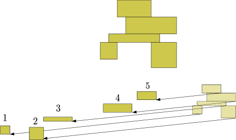
Choose two non-parallel directions and in , and assume that has a positive slope and has a negative slope. The arguments for the other cases are analogous. An easy observation shows that there is a robot such that the bottom-left quadrant defined by its top-right vertex does not overlap with any other robots. We can use a single move in the direction of to translate the center of to a point that is extremely far from the other robots. By repeating this argument, we can separate every pair of robots by any arbitrary distance of our choice using moves. We can also perform this operation starting from the end positions following the direction and we can place the one-to-last position of and the second position of , say on concentric circles of distances arbitrarily-large from each other, see Figure 1. Hence, each robot has now two positions that need to be connected. This is possible with moves per robot. In total, we incur at most moves to translate the robots in from their starting positions to their destinations.
Note that we do not care about the geometric complexity or the number of bits required to encode the intermediate positions as we only need to show an upper bound on the number of moves.
3.2 Axis-Aligned Motion in a Bounding Box
In this section, we present upper bounds on the number of axis-aligned moves in the case where the (serial/parallel) axis-aligned motion takes place within an axis-aligned bounding box , as opposed to the free plane. The crux of the proof is showing that if the instance is feasible (i.e., admits a schedule within ), then it admits a schedule whose length is upper bounded by a computable function of the number of robots.
Let be an instance of -Rect-MP-. Fix an ordering on the vertices of any rectangle (say the clockwise ordering, starting always from the top left vertex). For any two robots and , the relative order of w.r.t. is the order in which the vertices of , when considered in the prescribed order, appear relatively to the vertices of (considered in the prescribed order as well), with respect to each of the - and -axes. Note that the relative order of with respect to determines, for each vertex of , the relative position of the -coordinate (resp. -coordinate) of with respect to the -coordinate (resp. -coordinate) of each vertex of (e.g, with respect to , the relative position of a vertex of w.r.t. to a vertex of indicates whether ).
Definition 3.3.
Fix an arbitrary ordering of the 2-sets of robots in . A configuration of is a sequence indicating, for each 2-set of robots in , considered in the prescribed order, the relative order of with respect to . A realization of a configuration is an embedding of the robots in such that the relative order of any two robots in conforms to that described by and the robots in the embedding are pairwise nonoverlapping in their interiors.111We can alternatively use the notion of order types instead of configurations, but this would result in a much worse upper bound on the number of moves.
Proposition 3.4.
For any two realizations of a configuration , there is a sequence of at most valid moves within the bounding box that translate the robots from their positions in to their positions in .
Proof 3.5.
The sequence of moves consists of two contiguous subsequences, the first in the horizontal direction and the second in the vertical direction. For the first subsequence of moves, we partition the robots in into two subsets: those whose positions in have smaller -coordinates than their positions in , referred to as , and those whose positions in have larger or equal -coordinates than those in , referred to as . We sort the robots in in a nondecreasing order of the -coordinates of their left vertical segments, and those in in a nonincreasing order of the -coordinates of their right vertical segments. For each robot in , considered one by one in the sorted order, we translate it horizontally so that its left (or equivalently right) vertical segment is aligned with the vertical extension of its left (or equivalently right) vertical segment in . We do the same for the robots in . Since is rectangular, both and are in , and the translations are axis-aligned, it follows that all the aforementioned translations are within .
After each robot in has reached its vertical extension in , we again partition into two subsets, those whose top horizontal segments in are above theirs in , referred to as , and those whose top horizontal segments in are below theirs in , referred to as . We sort in nonincreasing order of the their top horizontal segments (i.e., in decreasing order of their -coordinates) and those in in nondecreasing order of their bottom horizontal segments. We then route the robots in each partition in the sorted order to its horizontal line in , and hence to its final destination.
It is obvious that the above sequence of moves has length at most , and that at the end each robot is at its final destination in . Therefore, what is left is arguing that no move in the above sequence causes collision. It suffices to argue that for the subsequence of horizontal moves; the argument for the vertical moves is analogous.
Let and be two robots that are translated horizontally. Suppose first that both and are moving in the same direction (either both in the direction of or ), say in the direction of . Assume, w.l.o.g., that is moved before , and hence, its left vertical segment has a smaller -coordinate than that of . Since is a realization of , and since we move the robots in the described sorted order, clearly cannot collide with when was translated horizontally while was stationary. Consider now the horizontal translation of . Since the relative position of and are the same in and , and since the vertical segments of are now positioned on their vertical lines in , if collides with during the translation of then the relative position of the vertical segments of with respect to those in (and hence, the relative positions of w.r.t. ) will have to change and will never change back. Since and have the same relative order in and , this collision cannot occur. The argument is similar when and are moving in opposite directions. This completes the proof.
Proposition 3.6.
Let be a feasible instance of -Rect-MP- or -Rect-CMP-. Then there is a schedule for of length at most .
Proof 3.7.
Since the upper bound on the number of serial moves is also an upper bound on the number of parallel moves, it suffices to prove the theorem for -Rect-MP-.
Suppose that is feasible and consider an optimal schedule for . Observe that there are five possible relative positions of any two axis-aligned rectangles along each of the two axes, and thus at most twenty five possible relative orderings for any two robots. It follows that the total number of (distinct) configurations is at most , where is the number of 2-sets of . Since the schedule under consideration is optimal, the same configuration can appear at most times in the schedule; otherwise, by Proposition 3.4, the schedule could be “shortcut” by considering a sequence of at most moves that would translate the robots from the realization of the first occurrence of such a configuration to its last occurrence, thus reducing the length of schedule and contradicting its optimality. It follows that there is a schedule for of length at most .
We note that the obtained upper bounds on the length of the schedule of a feasible instance already suggest an approach for obtaining FPT algorithms, namely that of enumerating all sequences of configurations and then checking their realizability. This approach results in much worse running times than the ones for the FPT algorithms presented in this paper, and reveals less about the structure of the solution than the presented results.
4 Axis-Aligned Motion
In this section, we prove a structural result about -Rect-MP. This result, in particular, and the upper bound on the number of moves imply that -Rect-MP is FPT parameterized by the number of robots. In brief, the structural result states that, in order to obtain an optimal schedule to an instance of -Rect-MP, it is enough to restrict the robots to move along the lines of an axis-aligned grid (i.e., a collection of horizontal and vertical lines of the plane), that can be determined from the input instance. Moreover, the number of lines in the grid is a computable function of the number of robots, and the robots’ moves will be defined using intersections of the grid lines.
Definition 4.1.
Let be an instance of -Rect-MP. We define an axis-aligned grid , associated with the instance , as follows.
-
•
Initialize to the set of horizontal and vertical lines through the starting and final positions of the centers of the robots in ; call these lines the basic grid lines.
-
•
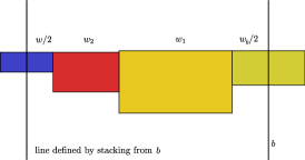
Add to the lines which are defined using “stackings” of robots on the basic lines as follows; see Figure 2. Let be a vertical basic line with -coordinate , and be the width of the robot whose center could be on . For each number , and each -multiset of robots, and for each choice of a horizontal width of a robot, add to the two vertical lines with -coordinates .
-
•
Add to the analogous lines for the horizontal basic lines.
Theorem 4.2.
Every instance of -Rect-MP has an optimal schedule in which every robot’s move is between two grid points along a grid line in . The number of vertical (resp. horizontal) lines in is at most .
Proof 4.3.
We argue by induction on the number of moves in the schedule. If , then the schedule has a single move that must be along a line defined by both the starting and ending positions of a robot in , and the statement is true in this case. Thus, assume henceforth that the statement of the theorem is true when the optimal schedule has at most moves. Let be the robot that performs the first move (in the schedule) from some point to some point , and assume, w.l.o.g., that the move is horizontal in the direction of . We define a new problem instance , which is the same as , with the exceptions that in the robot now has starting position and the upper bound on the number of moves is . Let and be the grids associated with instances and , respectively, as defined in Definition 4.1. The instance has a schedule of moves and hence, there is a schedule for such that each robot moves along a grid line in .
The lines in the set are basic vertical grid lines defined by being at plus all the lines defined by stackings of these lines. Note that contains only vertical lines and that . Let be the set of grid lines in union the set of vertical lines obtained by stacking every robot on every line in . Observe that , and that we are allowed to perform this additional stacking operation since the construction of involves stackings, whereas the construction of involves stackings.
From among all schedules of length for along the grid lines , consider a schedule that uses the maximum number of grid lines from .
Note that the move of from to and the schedule for give an optimal schedule for the original problem instance ; however, this schedule is not along the grid lines of , and some robots may move along the lines in .
Let be the set of segments of the grid lines in traversed by robot moves that are along the lines of ; note that all of these are vertical. Now we push back the robot from towards . Let denote the robot located at point . The move from to remains valid, however, there might be intersections between and other robots in future moves, and between this move and future positions of itself.
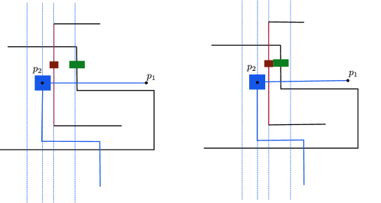
When , we have a schedule, and thus no collisions exist. From the construction of the grid lines, it follows that when the robot moves, the (updated) grid lines in move by exactly the same distance in the same direction. We now move all the segments of also in the same direction and distance, i.e., we move the grid lines in together with all the robot moves along them; see Figure 3. As we push back towards , we stop the first time that the right edge of some robot, say , that travels along a segment in , hits a vertical line that is defined by the left edge of a robot located on a line in , and hence cannot be pushed further without potentially introducing a collision. Now the center of is positioned at a line that is defined by some stacking of , and hence is a vertical line of . Since we have not introduced any collisions during the pushing, we have obtained a grid schedule that uses more grid lines from , which contradicts the maximality of the chosen schedule for . Therefore, there is a schedule in which all moves are along .
Finally, we upper bound the number of lines in the grid. We upper bound the number of vertical lines; the upper bound on the number of horizontal lines is the same. Let be the set of vertical lines in the grid, and be that of the horizontal lines.
The number of starting and ending positions of the robots is , and hence the number of basic vertical lines is at most . For each , where , and for each basic vertical line , we fix two robots: the one of width whose center could fall on and the one of width whose center could fall on the newly-defined vertical line based on the stacking. There are choices for these two robots. Afterwards, we enumerate each selection of an -multiset of robots, and for each -multiset , we add the two vertical lines with offset to the left and right of . Note that this offset is determined by the two fixed robots and the -multiset of robots, and hence by the two fixed robots and the set of robots in this multiset together with the multiplicity of each robot in this set. Therefore, in step , to add the vertical lines, we can enumerate every 2-set of robots, each -subset of robots, where , order the robots in the -set, and for each of the at most -subsets of robots, enumerate all partitions of into parts. The number of such partitions is at most . Hence, the number of vertical lines we add in step is at most , and the total number of vertical lines we add over all the steps is at most . It follows that and as well. Therefore, the total number of lines in the grid is .
Theorem 4.4.
-Rect-MP, parameterized by the number of robots, can be solved in time, and hence is FPT.
Proof 4.5.
By the above theorem and by Proposition 3.1, the total number of horizontal/vertical lines in the grid is . The algorithm enumerates all potential schedules of length at most along the grid. To do so, the algorithm enumerates all sequences of at most moves of robots along the grid lines. To choose a move, we first choose a robot from among the robots, then choose the direction of the move (i.e., horizontal or vertical), and finally choose the grid line in either (if the move is horizontal) or (if the move is vertical) that the robot moves to. The number of choices per move is at most . It follows that the number of sequences that the algorithm needs to enumerate in order to find a desired schedule (if it exists) is at most by Proposition 3.1. Since the processing time over any given sequence is polynomial, it follows that the running time of the algorithm is .
The following result is also a byproduct of our structural result, since one can, in polynomial time, “guess” and “verify” a schedule of length at most to an instance of -Rect-MP based on the grid corresponding to the instance:
Corollary 4.6.
-Rect-MP is in NP.
The above corollary will be complemented with Theorem LABEL:thm:nphard in Section LABEL:sec:nphardfixeddirections to show that -Rect-MP is NP-complete.
5 An FPT Algorithm When the Directions are Given
In this section, we give an FPT algorithm for the case of axis-aligned rectangles that serially translate along a given (i.e., part of the input) fixed-cardinality set of directions. We first start by discussing the case where the robots move in the free plane, and then explain how the algorithm extends to the case where the robots are confined to a bounding box.
Let be an instance of Rect-MP, where is a set of axis-aligned rectangular robots, and , where is a constant, is a set of unit vectors; we assumed herein that is a constant, but in fact, the results hold for any set of directions whose cardinality is a function of . Let be the coordinates of the initial position of the center of and be those of its final destination. We present a nondeterministic algorithm for solving the problem that makes a function of many guesses. The purpose of doing so is two fold. First, it will serve the purpose of proving the membership of Rect-MP in NP since the nondeterministic algorithm runs in polynomial time (assuming that is a constant or polynomial in ). Second, it will render the presentation of the algorithm much simpler. We will then show in Theorem LABEL:thm:lpfpt how to make the algorithm deterministic by enumerating all possibilities for its nondeterministic guesses, and analyze its running time.
At a high level, the algorithm consists of three main steps: (1) guess the order in which the robots move in a schedule of length (if it exists); (2) guess the direction (i.e., the vector in ) of each move; and (3) use Linear Programming (LP) to check the existence of corresponding amplitudes for the unit vectors associated with the moves that avoid collision.
We start by guessing the exact length, w.l.o.g. call it (since it is a number between and ), of the schedule sought. We then guess a sequence of events , where each event is a pair , , that corresponds to a move/translation of a robot along a vector in the sought schedule.
The remaining part of the algorithm is to check if there is a schedule of length that is “faithful” to the guessed sequence of events.
6 On the Visibility Regions
We are given robots . Each robot is a rectangle of fixed width and length , respectively, . We are also given start positions for robots, denoted and end positions . We assume that each coordinate of the the start and end positions is a rational number. The size of the input is the total number of bits that is used to encode the coordinates of the starting and end positions and the dimensions of the robots.
The
Problem 6.1.
problem asks to find the smallest number of translations that moves all of the robots from their starting positions to their end positions, and such that during the whole process no intersection happens between two robots. We denote the optimal number of moves by .
The feasibility region
Suppose we have an instance of the
Problem 6.2.
. Let be a -tuple of points. We now fix the endpoints . For each , the feasibility region (with respect to the fixed endpoints) is defined as
the plane by fixing all but one starting point. The feasibility regionof , fixing at , , is defined as
Let be an -tuple of numbers that gives the ordered sequence of the robots that move, potentially in an optimal solution for the problem instance . Given a sequence of moves , we can restrict the feasibility regionto those where the sequence of moves agrees with the given order. We call these sequences and . From now on, we write and for the sub-sequence obtained by removing . Therefore, we can write for short.
reachability
TO DO- This is same as visibility but considers only valid positions that the center of the robot can reach without causing intersection. The reach of a region is denoted as .
Determining feasibility region
It is possible to determine for all possible in terms of the end positions.
In this section we want to write formulas that express the sets for all possible in terms of for all possible . Notice that we are moving backwards from the end positions.
Assume that we know the sequence of move and that we know for all possible .
The sequence provides us with the robot that move at each step. Without loss of generality we assume that the robot that moves in the -th move is . moves from into in the forward direction. The rest of the robots are fixed at . We know that .
Lemma 6.3.
If robot moves in the -th move of an optimal solution with ordering , and other robots are fixed at , then
The above lemma describe the relation in an easy case (say why). The hard case is to update the feasibility region where the first robot is fixed. Let be a segment that the center of a robot traces in the th move. We defined the thickening of as , where is the robot at position .
Lemma 6.4.
If robot moves in the -th move of an optimal solution with ordering from to , and other robots are fixed at , then for
6.1 Moving along Fixed Directions
In this section, we prove that for Rect-MP- restricted to a fixed set of directions, under certain necessary conditions, we can obtain an upper bound on the number of moves that depends only on . The notion of a configuration is defined analogously to that for the axis-aligned case.
Proposition 6.5.
Let be a fixed set of directions. Consider an instance of Rect-MP- or Rect-CMP-. In addition, assume that the sizes of the robots in satisfy the following relation
where is the length of the longest side of the bounding box, and is the summation of longest sides of all the robots, and is a constant. Then, there is a constant (depending on and ) such that, for any two realizations of a configuration within , there is a sequence of at most valid moves that translate the robots from their positions in to their positions in .
Proof 6.6.
If all directions in are parallel, then clearly if the instance is feasibly then it has a schedule of length at most . So assume contains at least two non-parallel directions and . In the proof of Proposition 3.4, it was shown that two realizations and for the same configuration can be obtained from each other by a sequence of horizontal and vertical moves. We now prove that each of these moves can be simulated by a sequence of moves in the directions of and . W.l.o.g, we can assume that the move we are simulating is horizontal and to the left. We intend to replace the horizontal move by a zigzag of moves along and , see Figure LABEL:. If it turns out that and are close to each other, then we potentially need many zigs and zags. The directions are constant for us.11todo: 1Iyad: This is not clear. Also, it can be easily observed that the number of moves in the zigzag depends on the “width” of the passageway we need to cross.22todo: 2Iyad: This is not clear. To increase this width, we separate the robots as follows.
If the robot has already a non-zero vertical distance to all robots above it, or to all robots below it, we can replace the horizontal move by a sequence of zigzag moves where depends on the coordinates of the directions and the extensions of the robots. If there is a stack of robots touching each other on top of a robot that we want to move, and also a stack on bottom (imagine this as a “connected component” of robots), then at least one of these stacks must not touch the horizontal line of the bounding box, since then no move will be possible in a direction other than that direction is horizontal. W.l.o.g, assume that the stack on top of ends before the top edge of the bounding box. We first move the stack by at most moves a little away from (this can be done for instance by moving a robot whose upper and left edges do not touch anything first, and then repeat this process for the remaining component), and then perform moves to move to the left, and then move back the stack by at most moves to their original place. We therefore can simulate each horizontal move by moves where is constant depending on the bit-size of the directions and the extensions of the robots.
If the motion is not axis-aligned, we can only obtain FPT result for the case where is fixed and satisfies the conditions in Proposition 6.5:
Theorem 6.7.
Given an instance of Rect-MP- in which the box and satisfy the conditions in Proposition 6.5, in time , we can construct a solution to the instance or decide that no solution exists, and hence Rect-MP- is FPT.
7 Extension to Polygons
In this section, we show that the FPT algorithm for Rect-MP, presented in Section 5, can be extended to Rect-MP for any set of closed polygons such that the number of edges of each polygon is upper bounded by a constant, or even by any computable function of the parameter . The algorithm proceeds in the same fashion by guessing and then guessing the sequence of events. For a polygonal robot , a vector and , trace() is defined similarly, but now it can have at most edges. Therefore, to stipulate non-collision between and a robot , many pairs of segments need to be considered, each pair giving rise to four cases to guess from. By a similar analysis to that in the previous section, we have the following theorem:
Theorem 7.1.
Given an instance , where each robot in is a closed polygon with at most edges, for some computable function , in time , we can construct a solution to the instance or decide that no solution exists, and hence Rect-MP is FPT.
Corollary 7.2.
Let be an integer constant. The restriction of Rect-MP to instances in which each polygon has at most edges is in NP.