Efficient simulations of Hartree–Fock equations by an accelerated gradient descent method

Abstract

We develop convergence acceleration procedures that enable a gradient descent-type iteration method to efficiently simulate Hartree–Fock equations for atoms interacting both with each other and with an external potential. Our development focuses on three aspects: (i) optimization of a parameter in the preconditioning operator; (ii) adoption of a technique that eliminates the slowest-decaying mode to the case of many equations (describing many atoms); and (iii) a novel extension of the above technique that allows one to eliminate multiple modes simultaneously. We illustrate performance of the numerical method for the 2D model of the first layer of helium atoms above a graphene sheet. We demonstrate that incorporation of aspects (i) and (ii) above into the “plain” gradient descent method accelerates it by at least two orders of magnitude, and often by much more. Aspect (iii) — a multiple-mode elimination — may bring further improvement to the convergence rate compared to aspect (ii), the single-mode elimination. Both single- and multiple-mode elimination techniques are shown to significantly outperform the well-known Anderson Acceleration. We believe that our acceleration techniques can also be gainfully employed by other numerical methods, especially those handling hard-core-type interaction potentials.

I Introduction

The phases and phase transitions of system of adsorbed bosonic atoms on a substrate at low temperatures have received renewed attention due to the possibility of experimentally realizing a spatially modulated superfluid state for the second layer of bosonic ⁴He atoms on corrugated graphite substrates [1, 2, 3]. Here, the potential interplay between superfluidity and broken translational symmetry is argued to arise from a strong competition between these two types of orders. While some zero-temperature numerical simulations [4, 5] provide support for this scenario, other finite-temperature path integral quantum Monte Carlo results [6] find only incommensurate solid or superfluid phases. The origin of continuing uncertainty on the phase diagram in these few-layer adsorbed helium systems may be a result of the utilization of different adsorption potentials of different degrees of complexity [7, 8] combined with the complexity of performing full ab initio three-dimensional simulations of this strongly interacting system.

Seeking to reduce the complexity and enhance throughput of the determination of the adsorbed many-body wavefunction of ⁴He on corrugated substrates, we present a relatively simple and time-efficient gradient descent-type iterative method to solve Hartree–Fock (HF) equations that describe particles interacting with each other via hard core-type potentials (i.e., those leading to strong repulsion at short distances) as well as being influenced by an external adsorption potential. An early non-optimized version of the algorithm was employed in a recent study by two of the authors [9] seeking to determine a low-energy effective model for a single layer of ⁴He atoms adsorbed on a graphene membrane. Here we present the details of an improved algorithm, whose convergence is accelerated by preconditioning and slow-mode elimination, where the following main issues where addressed. First, we show how to optimize the preconditioning operator in the presence of a hard-core-type interatomic potential. Second, we show how the acceleration that relies on elimination of the mode decaying the slowest from one iteration to the next, should be carried out for multiple equations. Third, we present a novel extension of the above technique that eliminates several slowly decaying modes simultaneously.

We emphasize that our numerical technique is complementary to many existing HF-based electronic structure computations, which are designed to handle thousands of particles. Those approaches seek the solution of the many-body wavefunction as an expansion over a basis of localized functions [10, 11, 12, 13]. In contrast, the approach described in this paper is based on iteratively solving HF equations for smaller numbers of adsorbed particles, expanding them in the (nonlocal) Fourier basis. The value of our numerical approach is in the relative simplicity of its implementation compared to other numerical techniques. The novel contribution of this work is in significant acceleration of convergence of the gradient descent method, as well as in providing understanding of what factors slow down the non-accelerated method.

Anderson Acceleration [14], also known under the names Pulay Mixing and Direct Inversion of the Iteration Subspace, is a widely used acceleration technique for gradient descent-type methods in electronic structure calculations; see, e.g., [15, 16, 17] and references therein. We will show that our slow-mode elimination-based acceleration significantly outperforms the Anderson Acceleration. We also mention that in a recent paper [17], its authors demonstrated that an acceleration by the Heavy Ball algorithm, widely used in Optimization, significantly reduces the number of iterations of a gradient descent method applied to the so-called Energy Density Functional calculations of atomic nuclei. (The latter model is of the HF type, but more complicated.) However, optimal performance of this acceleration algorithm relies on having a satisfactory estimate for the condition number of the linearized iteration operator. While in [17] the authors were able to obtain such an estimate, it is unclear how to do so in other models, including that considered here. Optimization of performance of our acceleration techniques does not rely on knowing properties of the linearized iteration operator (other than it is Hermitian).

A number of other iterative methods for HF equations including quasi-Newton, fixed-point, and extrapolation-based methods were reviewed in, e.g., [15]. Examples considered there pertained to solving a Hartree-type equation for electrons in single light atoms, C and Na, and in a single diatomic molecule, CO. The baseline method was the standard gradient descent method, with the only kind of acceleration used being taking a weighted average between two successive values of the potential. In those examples, the number of iterations of the baseline method was under 50, and an extrapolation-based acceleration (the most efficient one of all types of acceleration considered there) reduced that number by some factor of two or less. In contrast, for the model considered in our study, the number of iterations of the baseline method (i.e., of the same non-accelerated method as used in [15]) is in the (many) tens of thousands. Our acceleration techniques reduce that number by at least two orders of magnitude, and often by much more.

The main part of this work is organized as follows. In Sec. II we present the HF equations and the general form of the numerical method used to solve them. In Sec. III, we begin by discussing specifics of the convergence acceleration technique used by the method, including an optimal choice of its parameters. This leads us to presenting, in Sec. IV, a non-trivial and novel generalization of the mode elimination technique, which allows one to eliminate multiple slow modes. In Sec. V, we use our numerical method to obtain results for the ⁴He atoms covering a graphene sheet at various filling fractions. Among those there are a few patterns which, to our knowledge, have not been depicted in the literature. We summarize in Sec. VI. We note that presentation in Secs. III and IV refers to a (non-physical) 1D model so as to focus on exposition of the underlying concepts of the numerical method. The same concepts apply to higher-dimensional generalizations of the method, and 2D results are presented in Sec. V. The reader who is interested only in the implementation steps of the numerical method can find them referenced compactly in Sec. VI. Appendices contain technical information that could be useful for either understanding or implementation of the methods discussed. Supplemental Material contains technical details that are less essential for the understanding and implementation than those found in the Appendices.

II Hartree–Fock equations and numerical method

II.1 Hartree–Fock equations

The model for which we will illustrate our numerical method is a system of ⁴He atoms (bosons) interacting with each other and with the graphene sheet above which they are located. Full determination of the wavefunction of $N$ bosons via Monte Carlo simulations is computationally costly. An alternative is to follow an approximate — HF — description, where the full wavefunction $\Psi$ is replaced with an ansatz:

$$\Psi({\bf r}_{1},{\bf r}_{2},\ldots,{\bf r}_{N})\,\,=\,\frac{1}{\sqrt{N!}}\,\sum_{{\rm symm},\,q}\;\;\prod_{j=1}^{N}\phi_{j}({\bf r}_{q}),$$ (1)

where ${\bf r}_{q}$ are the coordinates of particle $q$,  $j$ is the label of a quantum state where particle $q$ is found, and the summation is over all $N!$ permutations of the $N$ particles. Ansatz (1) assumes that the bosons, interacting via hard-core-type potential, cannot occupy the same spatial location, and therefore the aforementioned ‘state’ amounts to the location. The one-particle “wavefunctions” (in what follows we will drop the quotes) satisfy the orthonormality condition

$$\langle\phi_{i}|\phi_{j}\rangle\equiv\int_{\mathbb{R}^{2}}d^{2}{\bf r}\,\phi^{\dagger}_{i}({\bf r})\phi_{j}({\bf r})=\delta_{i,j}\,,$$ (2)

and $\dagger$ stands for Hermitian conjugation. Thus, wavefunctions of particles occupying different locations are orthogonal. It should be clarified that the functions $\phi_{i},\,\phi_{j}$ are scalars, and the transposition, implied by the $\dagger$, will be only used in the presentation of the numerical method below where some of the quantities will be vectors or matrices.

The wavefunctions $\phi_{i}$ can be shown to satisfy the HF equations (see, e.g., [18, 19]):

$$L_{0}\phi_{j}\;\equiv\;L_{00}\phi_{j}-\sum_{i}\langle\phi_{i}|\,L_{00}\phi_{j}\rangle\,\phi_{i}\;=\,0,$$ (3)

where

$$L_{00}\phi_{j}\equiv\left(-\nabla^{2}+V_{\rm ext}({\bf r})\,\right)\phi_{j}\,+\,\sum_{i\neq j}\langle\phi_{i}|\,V_{\rm int}\,|\phi_{i}\rangle\,\phi_{j}\,+\,\sum_{i\neq j}\langle\phi_{i}|\,V_{\rm int}\,|\phi_{j}\rangle\,\phi_{i},$$ (4)

$$\langle\phi_{i}|\,V_{\rm int}\,|\phi_{j}\rangle\equiv\int_{\mathbb{R}^{2}}d^{2}{\bf r}^{\prime}\,\phi^{*}_{i}({\bf r}^{\prime})\,V_{\rm int}({\bf r}-{\bf r}^{\prime})\,\phi_{j}({\bf r}^{\prime})\,.$$

Equations (3) arise from minimizing the Hamiltonian functional, whose variational derivative is the $L_{00}$-term, subject to the constraints (2), which give rise to the sum in (3), with $\langle\phi_{i}|\,L_{00}\phi_{j}\rangle$ being Lagrange multipliers. In deriving (4), one uses the fact that the particles (helium atoms in our case) are hard-core bosons, which cannot occupy the same site due to strong repulsion via the interaction potential $V_{\rm int}$. Also, $\nabla^{2}$ in (4) is the Laplacian and $V_{\rm ext}$ is the external potential; the third and fourth terms describe the mean-field (Hartree) and exchange (Fock) contributions, respectively. The spatial variables are nondimensionalized to some scale $d_{0}$, usually taken to be a period of $V_{\rm ext}$, and all energies are nondimensionalized to the recoil energy  $E_{R}=h^{2}/(8md_{0})$, where $h$ is the Planck constant and $m$ is the particle mass.

Potential $V_{\rm ext}$ describes the effect on helium atoms by the hexagonal lattice of graphene. It is obtained from the 3D Steele potential [7] as explained in [9]. This $V_{\rm ext}$ has the standard honeycomb shape with minima over the centers of the graphene cells and maxima over the carbon atoms. Focusing here on the numerical method rather than on fine aspects of the physical model, we use the simplest such shape:

$$V_{\rm ext}=V_{0}\,\left(\cos{\bf g}_{1}{\bf r}+\cos{\bf g}_{2}{\bf r}+\cos{\bf g}_{3}{\bf r}\right),$$ (5a)

$${\bf g}_{1}=\frac{2\pi}{d_{0}}\left[1,\frac{1}{\sqrt{3}}\right],\quad{\bf g}_{2}=\frac{2\pi}{d_{0}}\left[-1,\frac{1}{\sqrt{3}}\right],\quad{\bf g}_{3}={\bf g}_{1}+{\bf g}_{2};$$ (5b)

where the distance between centers of graphene cells is $d_{0}=2.46$Å and $V_{0}$ is chosen so as to yield $(V_{\rm ext})_{\max}-(V_{\rm ext})_{\min}=2.5E_{R}\approx 25$K, consistently with the value used in [9]. The recoil energy corresponding to the above $d_{0}$ is $E_{R}=9.9$K.

The helium–helium interaction potential $V_{\rm int}$ is taken from [20]. Its numerical modeling in (4) is discussed in Appendix A.1.

II.2 Numerical method

We will solve Eqs. (2), (3) by the Accelerated version of the Imaginary-Time Evolution Method (AITEM) given by Eqs. (6c)–(8c) below [21]:

$$(\phi_{j})_{n+1}=(\phi_{j})_{n}-\Delta t\,\left[P^{-1}\,\big{(}L^{(0)}\phi_{j}\big{)}_{n}-\Gamma_{{\rm slow},n}\;(u_{{\rm slow},j})_{n}\,\right],$$ (6a)

where $$n \Delta t>0 \big{(}L^{(0)}\phi_{j}\big{)}_{n} P^{-1}$$ is the iteration number, is an auxiliary parameter called the “imaginary time step,” is the modification of (3) that takes into account the preconditioning operator :

$$\big{(}L^{(0)}\phi_{j}\big{)}_{n}\;\equiv\;(L_{00}\phi_{j})_{n}-(\vec{\phi})_{n}\,\langle P^{-1}(\vec{\phi})_{n}\,|(\vec{\phi})_{n}\rangle^{-1}\,\langle P^{-1}\vec{\phi}\,|(L_{00}\phi_{j})_{n}\rangle\,,$$ (6b)

with

$$(\vec{\phi})_{n}\equiv\big{(}[\phi_{1},\phi_{2},\ldots,\phi_{N}]\big{)}_{n}\,;$$ (6c)

and the positive definite operator $P$ being chosen as

$$P=c-\nabla^{2}$$ (7)

for some constant $c>0$. The specific form of the second term on the r.h.s. of (6b) is derived in Supplemental Material based on the general formula presented in [21]. There we also show that equation  $L^{(0)}\phi_{j}=0$  is equivalent to Eq. (3).

The purpose of the $\Gamma$-term in (6a) is to perform mode elimination (ME), i.e., eliminate the slowest-decaying mode from the iterative solution [22]. This slowest mode is approximated by:

$$(u_{{\rm slow},j})_{n}=(\phi_{j})_{n}-(\phi_{j})_{n-1},$$ (8a)

and for a single equation (i.e., $$N=1 \phi_{1}\equiv\phi \Gamma_{{\rm slow},n}$$ and solution above), the coefficient is to be chosen as [22]:

$$\Gamma_{{\rm slow},n}=\gamma_{{\rm slow},n}\,\frac{\langle u_{{\rm slow},\,n}|\big{(}L^{(0)}\phi\big{)}_{n}\rangle}{\langle u_{{\rm slow},\,n}|P\,u_{{\rm slow},\,n}\rangle}\,,\qquad\quad\gamma_{{\rm slow},n}=1-\frac{s}{\alpha_{n}\Delta t},$$ (8b)

where $$\alpha_{n}$$ is an approximation of the eigenvalue of the slowest-decaying eigenmode. For the case of a single equation, one has

$$\alpha_{n}=\frac{\langle u_{{\rm slow},\,n}|Lu_{{\rm slow},\,n}\rangle}{\langle u_{{\rm slow},\,n}|Pu_{{\rm slow},\,n}\rangle}\,.$$ (8c)

The form of $\Gamma_{{\rm slow},n}$ and $\alpha_{n}$ for $N>1$ coupled equations (3) will be discussed in Sec. III. The parameter $s\in(\alpha_{n}\Delta t,1)$ in (8b) determines how much of the slowest mode is being subtracted at each iteration, with $s=\alpha_{n}\Delta t$ and $s=1$ corresponding to 0 and 100% of the mode, respectively. An optimal range for $s$ will also be discussed in Secs. III–V. Operator $L$ in (8c) is the linearized operator of (6b), defined as follows: If $\vec{\phi}$ satisfies (3) and $\|\widetilde{\vec{\phi}}\|\ll\|\vec{\phi}\|$, then in the linear approximation:

$$L^{(0)}\left(\vec{\phi}+\widetilde{\vec{\phi}}\;\right)\equiv L^{(0)}\vec{\phi}+L\widetilde{\vec{\phi}}=L_{0}\vec{\phi}+L\widetilde{\vec{\phi}}=L\widetilde{\vec{\phi}}\,,$$ (9)

where in the last step we have used (3). Per the note after (7), $L$ is also the linearized operator of $L_{0}$. Conveniently for the method, the $L$-term in (8c) does not need to be computed exactly but can instead be approximated by:

$$L(u_{{\rm slow},j})_{n}\approx\big{(}L^{(0)}\phi_{j}\big{)}_{n}-\big{(}L^{(0)}\phi_{j}\big{)}_{n-1}\,,$$ (8d)

assuming that $(\vec{\phi})_{n}$ is sufficiently close to the exact solution $\vec{\phi}$. (For future reference, we have written this relation for the case of multiple coupled equations, i.e., with the index $j$.) The final step of the iteration method is the Gram–Schmidt orthonormalization of $\phi_{j}$’s so as to ensure condition (2) to hold to numerical precision.

Seven remarks about the above numerical method are in order. First, the main contributions of this work, listed in the order in which they are discussed in Sec. III, are:  (i) Finding a range of values of parameter $c$ in (7) that significantly accelerates convergence of the iterations;  (ii)  Extension of the ME technique, i.e., the form of the $\Gamma$-term in (6a) and of the expressions in (8b) and (8c), from a single equation to a system;  and  (iii) Extension of the same technique that allows one to eliminate multiple slow modes simultaneously. Thus, there are two ways in which the textbook ITEM is accelerated by our AITEM (6a): via the preconditioning by operator $P$ and via ME by the $\Gamma$-term.

Second, a necessary condition for iterations (6a) to converge is that the eigenvalues of the linearized operator $L$ be positive. This cannot be guaranteed without knowing the solutions $\phi_{j}$. However, it was shown in [21] that if $\phi_{j}$ are dynamically stable (usually, ground-state) stationary solutions of time-dependent evolution equations  $i(\phi_{j})_{t}=L_{0}\phi_{j}$, where $L_{0}\phi_{j}$ is a Schrödinger-type operator, as in (3), and ‘$i$’ is the imaginary unit, then iterations (6a) without the $\Gamma$-term and for a sufficiently small $\Delta t$, do converge. In this case they will also converge with a properly designed $\Gamma$-term, since it does not change the sign of eigenvalues of the linearized operator $L$ but effectively changes only the magnitude of the slowest-decaying eigenmode of $L$ [22].

Third, parameter $\Delta t$ needs to be chosen to satisfy a relation:

$$\Delta t<2/\max\lambda_{P^{-1}L}$$ (10)

so as to ensure convergence of the iterations; see, e.g., [23]. The denominator in (10) is the maximum eigenvalue of operator $P^{-1}L$. Since this eigenvalue is usually not known, $\Delta t$ is chosen empirically from a small number of trial simulations. More will be said about this in Sec. III.

Fourth, for periodic boundary conditions, which we use in this study, the Laplacian operator in (4) and (7) is efficiently computed using the Fast Fourier Transform. An efficient computation of the $V_{\rm int}$-terms is discussed in Appendix A.1.

Fifth, the exchange interaction between helium atoms (the Fock term in (4)) is much weaker than the mean-field interaction (the Hartree term). Therefore, one does not need to compute the Fock term until the iteration error becomes comparable in size to it. This can be monitored by computing the exchange interaction between any one pair of neighboring atoms every so many (say, $O(10)$) iterations and comparing it to the mean-field interaction between the same two atoms. Moreover, the Fock term is also more expensive to compute, as its computation scales with the number of helium atoms as $O(N^{2})$, whereas the computation of the Hartree term can be implemented to scale as $O(N)$ (see Appendix A.1). Therefore, we used a well-known method from molecular dynamics (see, e.g., [24, 25]) whereby this small but expensive term is computed only every $n_{\rm Fock}\gg 1$ iterations, in between which one uses its latest computed value. Furthermore, we verified for a number of selected cases (for high filling fractions) that using any value $n_{\rm Fock}$ from 1 to infinity (i.e., not including the Fock term at all) makes very little difference for the final solution: it changed the central peak of the wave functions by a negligible amount and the much weaker side peaks (see, e.g., Fig. 7 in [9]), by some 10–20%.

Sixth, the Conjugate Gradient Method (CGM) is known to be the fastest generic fixed point-type method for problems with Hermitian positive definite operators, as far as the iteration count is concerned. An extension of the CGM to nonlinear wave equations with quadratic constraints, such as (2), was presented in [26]. We tried to employ this method instead of the simpler AITEM (6c)–(8c), but did not succeed. First and most importantly, the CGM iterations diverged. While we did not understand the reason for that divergence, we hypothesized that it could be intrinsic to how the iteration method “chooses” increments of the solution for the next iteration. Indeed, method (6c)–(8c), which is a gradient decent-type method, chooses those increments so as to, essentially, minimize energies of the helium atoms. This prevents such increments that lead to a (significant) increase of the $V_{\rm int}$-terms and thus keeps the overlap of neighboring $\phi_{j}$’s to a minimum. On the other hand, increments chosen by the CGM are designed to explore a wider range of directions [27]. As a result, they can potentially cause neighboring $\phi_{j}$’s to overlap to such an extent that the nearly singular behavior of $V_{\rm int}(|{{\bf r}}|)$ near ${\bf r}=0$ would lead to a sharp increase in the $V_{\rm int}$-terms and could thus cause divergence of iterations.  Second, while the CGM requires a factor of two to three fewer iterations to converge than the ME-accelerated method (6c)–(8c) [26], the cost of each iteration may be more than twice greater for the CGM. This is due to two factors:  (i)  The CGM computes both $L^{(0)}\phi_{j}$ and $L$ acting on some auxiliary quantity (versus one $L^{(0)}\phi_{j}$ for the AITEM), as well as computes two constraint-enforcing terms (those with angle brackets in (6b)), per iteration. (ii)  Moreover, the linearized operator $L$ must be computed explicitly, contrary to that in (8d). In examples considered in [26], nonlinear terms had much simpler form than the $V_{\rm int}$-terms in (4) and evaluation of the corresponding terms in $L$ was not the most computationally expensive part of an iteration. In contrast, not only are the $V_{\rm int}$-terms in (4) the most expensive ones to evaluate, but also their linearization is quite cumbersome to code. Thus, even if CGM iterations had converged, their computational time might not had been less than that of the simpler method (6c)–(8c), and the coding of the CGM is significantly more complex.

Finally, we chose to use a fixed point-type method over a Newton-type one, considered, e.g., in [15], because for the former methods, it is straightforward to compute spatial derivatives using the time-efficient and spectrally accurate Discrete Fourier transform, whereas it is not possible to do this time-efficiently for Newton-type methods.

II.3 Initial condition for the iterations

The ratio of the number $N$ of helium atoms and the number $N_{\rm cells}$ of graphene cells defines the filling fraction, $f\!f$, of the lattice by the atoms. Examples of commensurate $f\!f=1$ and $f\!f=1/3$ are shown in 1; examples of incommensurate filling fractions, where helium atoms are not located over the centers of the graphene cells, will be presented in Sec. V. The lattice has periodic boundary conditions to ensure consistency with the discrete Fourier transform used to compute the $\nabla^{2}$- and nonlocal terms in (4); see Appendix A. Due to this periodicity, non-unit filling fractions impose restrictions on the number of periods of the lattice. For commensurate filling fractions, these restrictions can be found by inspection. For example, for $f\!f=1/3$, one needs to have the number of cells in the $x$-direction, $N_{{\rm cells},\;x}$, be a multiple of 3. (Note that in Fig. 1, this restriction is violated intentionally in order to illustrate that without it, $f\!f=1/3$ could not be realized with periodic boundary conditions.) For other filling fractions to result in periodic patterns, restrictions on $N_{{\rm cells},\;x}$ and $N_{{\rm cells},\;y}$ need to be found by trial and error on a case-by-case basis; see Sec. V for examples. In addition, forall filling fractions, one needs to have $N_{{\rm cells},\;y}$ to be a multiple of 2 in order to fit a hexagonal lattice to a rectangular computational window while respecting periodic boundary conditions.

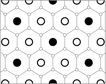
Figure 1: Schematics of helium atoms over a hexagonal graphene lattice. Small (large) circles denote carbon (helium) atoms. Thin lines are used to improve visibility of the lattice. Filled circles show the $1/3$-filling of the lattice by helium.

For the helium-over-graphene system considered here, fillings fractions with high $f\!f$ are only relevant for a strictly 2D system. In 3D simulations, or in experiments, a second layer of helium atoms begins to form above the first one for $f\!f\approx 0.62$ (equivalently, for area coverage of about 0.118 Å^-2) [28, 4, 29] over either graphite or graphene. To prevent this from occurring and thereby achieve higher values of $f\!f$ in 3D simulations, one would restrict the motion of helium atoms away from the surface by placing a “cap” on the simulation box, as was done in Ref. 9. In the 2D model considered here, we can meaningfully study filling fractions in the entire range $f\!f$ between 0 and 1.

To create an initial condition $(\phi_{j})_{0}$ for unit-filling simulations, one places identical copies of a 2D Gaussian function (with width of about a quarter of the lattice side) at the center of each graphene cell. For a non-unit filling $p/q$, we experimented with two alternative initial placement procedures of the aforementioned Gaussian. These details are described in Appendix A.3. The initial placement of helium atoms does not need to be (and in most cases is not) close to that obtained at the outcome of the simulation, as the equations themselves will “dictate” the equilibrium placement of the atoms.

III Choosing parameters of the numerical method

In Sec. III.1, we will discuss an optimal choice of parameter $c$ in the preconditioning operator $P$ (7). In Sec. III.2 we will discuss the form of the slow mode-eliminating term (the $\Gamma$-term) in (6a) for the case of multiple coupled equations. In Sec. III.3 we will demonstrate that ME accelerates the “original” AITEM (i.e., method (6c) without the $\Gamma$-term) by well over an order of magnitude. However, we will also reveal a problem of convergence of this ME-accelerated AITEM, which we will seek to overcome by presenting a novel, multiple-mode eliminating technique in Sec. IV.

The discussions in Secs. III.1,III.2 rely on the following well-established fact. Consider a fixed point iteration method whose linearized form is

$$\vec{q}_{n+1}=\vec{q}_{n}-\Delta tA\,\vec{q}_{n},$$ (11)

where $\vec{q}$ is the iterated quantity and $A$ is a Hermitian positive definite matrix; compare with (6a). Quantity $\vec{q}$ can be expanded over the set of eigenvectors $\vec{a}_{i}$ of $A$:  $\vec{q}=\sum_{i}b_{i}\,\vec{a}_{i}$, where the expansion coefficients in subsequent iterations satisfy:

$$(b_{i})_{n+1}=(1-\Delta t\lambda_{A,i})(b_{i})_{n},$$ (12)

with $\lambda_{A,i}$ being eigenvalues of $A$. Based on (12), convergence rate of (11) for an optimal choice of $\Delta t$ can be shown to be (see, e.g., [23] or references in [26]):

$$\frac{\|\vec{q}_{n}\|}{\|\vec{q}_{n+1}\|}=\frac{1+(\lambda_{A})_{\min}/(\lambda_{A})_{\max}}{1-(\lambda_{A})_{\min}/(\lambda_{A})_{\max}},$$ (13)

Thus, to ensure the fastest convergence of (11) with a (nearly) optimal $\Delta t$, one needs to modify $A$ so as to minimize ${\rm cond}A\equiv(\lambda_{A})_{\max}/(\lambda_{A})_{\min}>1$.

In the context of iteration method (6c), the role of $A$ is played by $P^{-1}L$, where $L$ is the linearized operator introduced in Sec. II.2. It is not feasible to find $\lambda_{P^{-1}L}$ for the 2D problem (3)–(6c). Therefore, for the purposes of convergence analysis of the AITEM, we considered a 1D and Hartree-only reduction of the instead, for which we were able to find those quantities numerically for a small number of atoms $N$. Those numerics used the idea of plane-wave expansion of the eigenfunctions of a Shrödinger-type operator (see, e.g., [30]), but were more technically complex due to the presence of the second term on the r.h.s. of (6b) and the nonlocal nonlinear terms in (4). Since details of those numerical implementations are not central to this work, we omit them and below will present only the setup (in this paragraph) and the results (in Secs. III.1,III.2). The Hartree-only reduction implies dropping the Fock term in (4) and using only $N$ normalization conditions (2) with $i=j$:

$$L_{0}^{\rm 1D,H}\phi_{j}\,\equiv\,L_{00}^{\rm 1D,H}\phi_{j}-\langle\phi_{j}|\,L_{00}^{\rm 1D,H}\phi_{j}\rangle\,\phi_{j}\;=\,0,\qquad\langle\phi_{j}|\phi_{j}\rangle=1,$$ (14a)

$$L_{00}^{\rm 1D,H}\phi_{j}\equiv\left(-\partial_{x}^{2}+V_{\rm ext}({\bf r})\,\right)\phi_{j}\,+\,\sum_{i\neq j}\langle\phi_{i}|\,V_{\rm int}\,|\phi_{i}\rangle\,\phi_{j}\,.$$ (14b)

The discrete version of $P^{-1}L$ is a $NM_{x}\times NM_{x}$ matrix, where $M_{x}$ is the number of grid points. For the results below, we chose, as representative values:

$$V_{\rm ext}=-2\cos(2x),\qquad E_{\rm clip}=100\;\mbox{(see Appendix A)}$$ (15)

in nondimensional units.

For the purpose of illustrating the behavior of the AITEM (6c), all examples considered in this section will be for the 1D, Hartree-only, model (14), (15). The behavior of the AITEM for the 2D HF model (2)–(4) are qualitatively the same. The results for it will be presented in Sec. V.

III.1 Optimal value of $c$ in (7)

The role of $P^{-1}$ is to reduce large eigenvalues of $L$ associated with high wavenumbers $k$ (see, e.g., [23]); the same preconditioning is widely used in computational condensed matter and nuclear physics: see, e.g., [17] and references therein). While the concept of preconditioning (7) is well-known, the question of an optimal $c$ value has not been, to our knowledge, systematically explored. We are aware of only one such study, [23], where an optimal $c$ value was found for a different class of problems and led to a different result than the one found below.

Large eigenvalues of $L$ occur due to the Laplacian in (4) whose contribution to the large-$k$ eigenvalues (with corresponding eigenfunctions containing fast oscillations) dominates that of the $V_{\rm ext}$- and $V_{\rm int}$-terms. Those eigenvalues of $P^{-1}L$ can be roughly estimated to be:

$$\lambda_{P^{-1}L}(|k|\gg 1)\sim(k^{2}+O(V_{\rm ext})+O(V_{\rm int}\mbox{-term}))/(k^{2}+c).$$ (16)

An expression for the ‘$V_{\rm int}$-term’ is given in Appendix B. When the Laplacian dominates the contributions of the $V_{\rm ext}$- and $V_{\rm int}$-terms (and the value of $c$), the above estimate is $O(1)$. If we now, as an initial motivation, assume that this estimate also holds, in the order of magnitude sense, for all eigenvalues, then we get:  $\lambda_{P^{-1}L}(|k|\lesssim 1)\sim(O(V_{\rm ext})+O(V_{\rm int}\mbox{-term}))/c$. This suggests that if  $|V_{\rm int}\mbox{-term}|\gg 1$, then one needs to have $c=O(V_{\rm int}\mbox{-term})$ in order to have $\lambda_{P^{-1}L}(\,|k|=O(1)\,)=O(1)$ also (here we have used that $V_{\rm ext}=O(1))$. We stress that the above order-of-magnitude estimate provides only an initial motivation for the choice of $c$. Moreover, it is not possible to estimate the $V_{\rm int}$-term without actually computing eigenfunctions of $P^{-1}L$ (see Appendix B), and that computation requires one to assume a specific value of $c$ in $P$.

To break this circular logic, we instead examined the size of entries of the $NM_{x}\times NM_{x}$ matrix $P^{-1}L$. Representative results are shown in Fig. 2. This matrix appears to be diagonally dominant (if not in the strict mathematical sense, then in appearance). The Gerschgorin Circles theorem implies that for a diagonally dominant matrix $A$, a necessary (but not sufficient) condition for ${\rm cond}A$ to be $O(1)$ is that the entries along the diagonal be uniform. From Fig. 2, one sees that this occurs only when

$$c=O(E_{\rm clip}).$$ (17)

This implies that for an optimal acceleration with the preconditioner $P^{-1}$, one needs to choose $c$ according to (17).

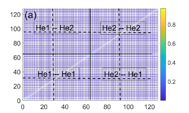
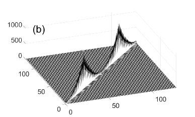
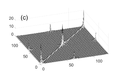
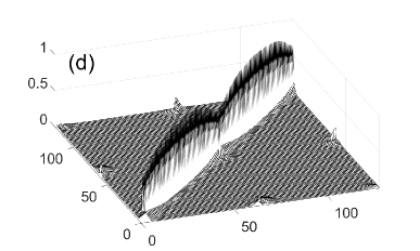
Figure 2: Absolute values of entries of $P^{-1}L$ for $N=2$ helium atoms in two adjacent wells of $V_{\rm ext}$ (15); $M_{x}=64$.  (a)  Top view of panel (d), to illustrate the matrix structure: solid lines separate the blocks pertaining to atom $i$’s eigenfunction contributing to atom $j$’s linearized equation (14a), as marked; dashed lines separate the two parts of the wavenumber vector, as per (41). Panels (b,c,d) show the entries for $P=I$ and $P$ given by (7) with $c=2$ and $c=100$, respectively.

To confirm this, we computed ${\rm cond}(P^{-1}L)$ for the examples shown in Fig. 2. When $P=I$ (no preconditioning), $\lambda_{\min}\approx 0.61$, $\lambda_{\max}\approx 1100$, ${\rm cond}(P^{-1}L)\approx 1800$. For $P$ with $c=2$ (a representative value of order $O(V_{\rm ext})$, as previously found in [23] in the context of nonlinear wave equations), $\lambda_{\min}\approx 0.030$, $\lambda_{\max}\approx 35$, ${\rm cond}(P^{-1}L)\approx 1150$. For $P$ with $c=100=E_{\rm clip}$, $\lambda_{\min}\approx 0.052$, $\lambda_{\max}\approx 0.98$, ${\rm cond}(P^{-1}L)\approx 19$.

Figure 3(a) illustrates that for high filling fractions, i.e., $f\!f\lesssim 1$, $c$ can be in a rather wide range (17) and still provide superior performance over the case where $c=O(1)$. Method (6c) without the $\Gamma$-term was used to iterate Eqs. (14) for $N=20$ helium atoms initially placed exactly at the centers of $N$ adjacent wells of $V_{\rm ext}$:

$$(\phi_{j})_{0}=\exp\left[-(x-x_{j})^{2}/w_{0}^{2}\right],$$ (18)

where $x_{j}$ are the locations of $V_{\rm ext}$’s minima and the width $w_{0}=0.2\pi$. The exact value of the width is not important as long as the initial Gaussians do not overlap; the importance of the italicized clause in the previous sentence and the absence of the need to include the $\Gamma$-term in (6c) in this case will be explained in Sec. III.2. The values of parameter $\Delta t$ for $c=50,100,200$ were not optimized. We merely checked that $\Delta t_{100}=0.6$ worked for $c=100$ and then used $\Delta t=0.5\Delta t_{100}$ and $\Delta t=2\Delta t_{100}$ for $c=50$ and $c=200$, respectively. This was motivated by the rough estimate (16), which along with (10) suggested that $\Delta t$ increases with $c$ (again, this is just a very approximate estimate). The point of not optimizing $\Delta t$ was to emphasize that method (6c) with a preconditioner $P$ where $c$ satisfies (17), does not require fine-tuning of $\Delta t$ to yield a much faster convergence than when $c=O(1)$. On the contrary, for $c=2$ in Fig. 3(a), we used a (nearly) optimal $\Delta t=0.025$, which we had found by trial and error. The main conclusion is that for sufficiently high filling fractions (with $f\!f=1$ considered above as an example), a value of $c$ satisfying (17) improves the convergence rate by at least on order of magnitude and likely more, given that we did not optimize $\Delta t$ for those $c$ values.

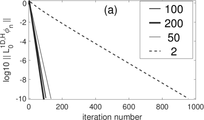
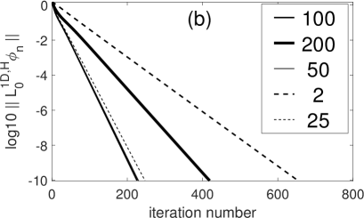
Figure 3: Evolution of the error in iterated Eqs. (14) for $N=20$ (a) and $N=10$ (b) equidistant helium atoms at $V_{\rm ext}$’s 20 minima. Here and below the error norm is defined as:  $\|L_{0}^{\rm 1D,H}\phi_{n}\|\equiv\sqrt{\int dx\sum_{j=1}^{N}|L_{0}^{\rm 1D,H}(\phi_{j}(x))_{n}|^{2}}\,/N$. See main text for more details. The values of $c$ are listed in the legend. In (b), the thin and medium solid lines are indistinguishable. Also, in (b) unlike in (a), all $\Delta t$ values were optimized by trial and error, and the corresponding values are $\Delta t=2.02,2.20,1.02,0.044,0.52$ for $c=100,200,50,2,25$, respectively.

For low filling fractions, we have found that an optimal value of $c$ is still in the range (17). However, the sensitivity of the convergence rate on $c$ is weaker than for $f\!f=1$, considered above. Figure 3(b) shows the error evolution for $f\!f=1/2$, which is the largest commensurate filling with $f\!f<1$ in 1D, with $\Delta t$ being optimized for each value of $c$. The conclusions for such low (see below) filling fractions are:  (i) The convergence rate for the optimal $c$ is only some factor of three better than for a suboptimal $c=O(1)$;  and  (ii)  It may be advisable to choose $c$ in the lower part of range (17), contrary to the case of higher filling fractions.

We conclude this subsection with two comments. First, $f\!f=1/2$ in 1D corresponds to $f\!f=(1/2)^{2}=1/4$ in 2D, which is lower than the commensurate filling with $f\!f=1/3$ in 2D. All filling fractions that we consider in Sec. V are greater than 1/3. Based on Fig. 3, we then set

$$c=E_{\rm clip}$$ (19)

in all simulations presented in this work and do not optimize $\Delta t$, as we focus on other aspects of convergence acceleration.  Second, the relatively low iteration count, in the low hundreds, suggested by Fig. 3, is due to the initial guesses (18) for the wavefunctions $\phi_{j}$ being centered precisely at the minima of $V_{\rm ext}$. When this restriction is lifted (which can be avoided only for a small minority of filling fractions such as 1, $1/3$, and a small number of others), the iteration count goes up by well over an order of magnitude and sometimes much more. This, as well as the ME-based acceleration technique required to overcome this problem, is considered in the next subsection.

III.2 Form of the $\Gamma$-term in (6a)

In this subsection we will motivate and present the form of the $\Gamma$-term in (6a) for the case of multiple equations, as in (3). Recall that in (8c) in Sec. II.1 that term was presented for a single equation, as introduced in [22].

The dashed line with circles in Fig. 4 shows the error evolution for the same setup as in Fig. 3(a), but when in the initial condition (18) the atoms are shifted slightly (by $\sim 1$% of $V_{\rm ext}$’s period) by random amount from the minima of their respective potential wells. The iterations converge to the same accuracy as in Fig. 3 in 4930 iterations, i.e., about 50 times slower than in the case when initial conditions are centered exactly at the minima of the wells. The culprit, then, must be a mode, or modes, of the linearized operator $P^{-1}L$ which are related to shifts of the atoms from their equilibria (i.e., the wells’ minima) and which must have much smaller eigenvalues than the other modes, as per (12). It is those modes that will need to be eliminated by an appropriately chosen $\Gamma$-term in (6a). The question is then:  Should one eliminate those “shift” modes one per atom, or are there certain combinations of the shifts that compose the slow (i.e., slowly decaying) modes? In the latter case, it would be those combinations that need to be eliminated.

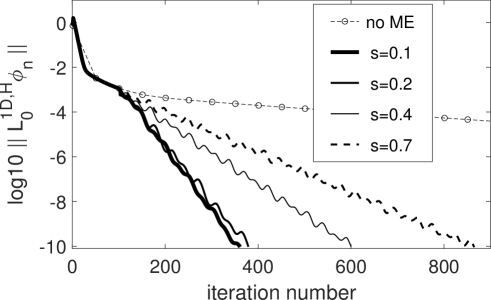
Figure 4: Error evolution for the same setup as in Fig. 3(a) with $c=100$, $\Delta t=0.6$, but when in the initial condition (18) the atoms are shifted by small random amounts from the minima of $V_{\rm ext}$. The line with circular symbols shows the behavior of iteration method (6c) without the $\Gamma$-term (no slow mode elimination); the other lines show the behavior of the same method with the $\Gamma$-term for different values of parameter $s$. In those cases, ME was started at the 100th iteration. Starting it at another iteration between 50th and 200th did not change the results significantly.

The answer to that question is inspired by Fig. 5. A unique mode with the lowest eigenvalue corresponds to a common shift of all helium atoms. (To see that component $j$ of this eigenfunction corresponds to a shift of atom $j$, think about the shape of the derivative of wavefunction $\phi_{j}$, which is qualitatively similar to (18), with respect to its center $x_{j}$.) The next eigenfunction, corresponding to two groups of the atoms shifting out of sync, has a much larger (by almost 20 times) eigenvalue. Higher modes in that figure correspond to “breathing” (width–amplitude changes) of $\phi_{j}$’s and its combinations with shifts. A discussion about why the common shift corresponds to the lowest-$\lambda$ eigenfunction for the system in question, is found in Appendix C.1.

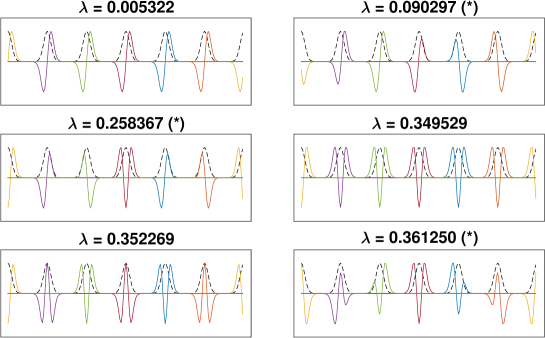
Figure 5: Eigenfunctions of $P^{-1}L$ with $c=100$ for $N=6$ helium atoms placed in $N$ adjacent wells of $V_{\rm ext}$, corresponding to its first few smallest eigenvalues. Thin dashed lines show the locations of the helium atoms. Vertical scale is in arbitrary units. The modes with asterisks next to the $\lambda$ value are doubly repeated. In those cases, the second eigenfunction (not shown) is obtained from the first by a shift by one period of $V_{\rm ext}$.

Thus, based on the above, the $\Gamma$-term must eliminate a single mode common to all $\phi_{j}$’s. Then, the following expressions replace their counterparts in (8b), (8c):

$$\Gamma_{{\rm slow},n}=\gamma_{{\rm slow},n}\,\frac{\sum_{j=1}^{N}\langle(u_{{\rm slow},\,j})_{n}|\big{(}L^{(0)}\phi_{j}\big{)}_{n}\rangle}{\sum_{j=1}^{N\vphantom{{T}}}\langle(u_{{\rm slow},\,j})_{n}|P\,(u_{{\rm slow},\,j})_{n}\rangle}\,\equiv\,\gamma_{{\rm slow},n}\,\frac{\langle\big{(}\overrightarrow{u_{\rm slow}}\big{)}_{n}^{T}\,|\,\big{(}L^{(0)}\vec{\phi}\big{)}_{n}^{T}\rangle}{\langle\big{(}\overrightarrow{u_{\rm slow}}\big{)}_{n}^{T\vphantom{{T}}}\,|\,\big{(}P\,\overrightarrow{u_{\rm slow}}\big{)}_{n}^{T}\rangle};$$ (20a)

with $$\gamma_{{\rm slow},n}$$ still being given by (8b), and where now

$$\alpha_{n}=\frac{\sum_{j=1}^{N}\langle(u_{{\rm slow},\,j})_{n}|L(u_{{\rm slow},\,j})_{n}\rangle}{\sum_{j=1}^{N\vphantom{{T}}}\langle(u_{{\rm slow},\,j})_{n}|P(u_{{\rm slow},\,j})_{n}\rangle}\,\equiv\,\frac{\langle\big{(}\overrightarrow{u_{\rm slow}}\big{)}_{n}^{T}\,|\,\big{(}L\,\overrightarrow{u_{\rm slow}}\big{)}_{n}^{T}\rangle}{\langle\big{(}\overrightarrow{u_{\rm slow}}\big{)}_{n}^{T\vphantom{{T}}}\,|\,\big{(}P\,\overrightarrow{u_{\rm slow}}\big{)}_{n}^{T}\rangle}.$$ (20b)

Here $\overrightarrow{u_{\rm slow}}$ is a vector defined from its components (8a) similarly to (6c).

The error evolution of such an ME-accelerated AITEM (6c) is shown in Fig. 4 for several representative values of parameter $s$ (see the text after (8c)). We note that in the case of a single equation [22], a relatively large value $s=0.7$ was advocated as optimal. In contrast, here, much smaller values $s\in[0.1,0.2]$ are shown to result in a considerably faster convergence. We hypothesize that the smaller values of $s$ being optimal here is related to the fact that the (preconditioned) linearized operator $P^{-1}L$ is still quite stiff, with ${\rm cond}\,(P^{-1}L)=\lambda_{\max}/\lambda_{\min}\approx 1.8/0.0053>300$.

An important note is in order about what mode is eliminated by the ME. Initially, i.e. right after the ME is started, it is the mode with the smallest eigenvalue of $P^{-1}L$ (or a combination of a few such modes if their eigenvalues are close to one another). Indeed, it is that mode which, in the absence of the $\Gamma$-term in (6a), “survives” the longest in the iteration error and hence dominates $(u_{{\rm slow},\,j})_{n}$ in (8a). However, after the ME has been applied for several tens of iterations, the contribution of those lowest-$\lambda$ modes to $(u_{{\rm slow},\,j})_{n}$ is reduced (by design), and the latter becomes a mix of several low-$\lambda$ modes, with $\alpha_{n}$ representing some kind of weighed average of the eigenvalues of those modes at iteration $n$. This mix of modes and, hence, $\alpha_{n}$ vary from one iteration to the next. This will be illustrated in Sec. IV.2.

Concluding this subsection, we mention that for commensurate filling fractions smaller than 1 in 1D, the benefits of ME for AITEM (6c) are slightly less pronounced. For $f\!f=1/2$, considered in Fig. 3(b), the AITEM with $c=100$, $\Delta t=0.6$ and without ME converges in about 1450 iterations when initial conditions are offset from $V_{\rm ext}$’s minima. ME with $s\in[0.1,0.3]$ brings the iteration count below 300. This 5-fold improvement should be compared to the more than 10-fold one for $f\!f=1$, as shown in Fig. 4. A brief discussion of this is found in Appendix C.1. We observed a similar relation between iteration counts for $f\!f=1/3$ and $f\!f=1$ in 2D. It is then surprising that for incommensurate $f\!f<1$, the benefits of ME can be much greater. This is demonstrated in the next subsection.

III.3 Performance of the ME-accelerated ITEM in 1D

Here we will examine performance of AITEM (6c), (20) for two incommensurate filling fractions. Our findings will, on the one hand, confirm a very significant benefit of ME for convergence acceleration, but, on the other, highlight a problem, which will be dealt with in the next section.

Figure 6 shows the evolution of the error and the total energy of Eqs. (14):

$$E_{\rm tot}=\sum_{j=1}^{N}\int_{\mathbb{R}^{2}}\,\left(\,\left(\partial_{x}\phi_{j}\right)^{2}+\frac{1}{2}V_{\rm ext}\,\phi_{j}^{2}+\frac{1}{2}\langle\phi_{j}\,|\,\sum_{i\neq j}\langle\phi_{i}|\,V_{\rm int}\,|\phi_{i}\rangle\,\phi_{j}\,\rangle\,\right)dx$$ (21)

obtained by AITEM (6c) without ME for 30 periods of $V_{\rm ext}$ and $N=23$ and $N=24$ helium atoms. The initial conditions are (18) with $x_{j}$ uniformly placed in the computational window. We used the same simulation parameters as those used in Sec. III.2 and listed in the caption to Fig. 4. Not optimizing parameters $c$ and $\Delta t$ of the AITEM, as well as the ME parameter $s$ mentioned later, was a deliberate choice made so as to focus on other issues.

The error in the $N=24$ case ($f\!f=0.8$) exhibits a peculiar behavior: After dropping to almost $10^{-5}$ in a couple thousand iterations, it then slowly climbs up almost 2 orders of magnitude before decaying again. The total energy (21) decays monotonically, with the local maximum of the error corresponding to an inflection point of the energy curve. Note that the energies of the intermediate solutions corresponding to points labeled ‘1’ and ‘2’ are $O(1)$ greater than that of the final solution. Moreover, the differences of the solutions $\phi_{j}$ themselves at these points from the final solution amount to a common shift of all atoms (similar to the first panel in Fig. 5 but with slightly non-uniform amplitudes) of sizes around 0.5 and 0.25, respectively (i.e., both also being $O(1)$). Interestingly, the difference from the final solution at point ‘2’ is smaller than the difference at point ‘1’, even though the error at ‘2’ is greater. In other words, even though the error (of the equations) exhibits a non-monotonic evolution, the iterated solution appears to approach the exact solution monotonically.

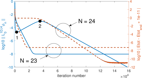
Figure 6: Error (solid lines) and total energy (dashed lines) evolutions of the AITEM (6c) without the $\Gamma$-term. See main text for more details. In the $y$-label of the right axis, the subscript ‘end’ refers to the last iteration in each of the two cases:  $\sim 158$ thousandth iteration for $N=24$ and $\sim 115$ millionth iteration for $N=23$, when the equation error reaches $10^{-10}$. The term $10^{-11}$ is added to the argument of the logarithm to avoid running into $\log 0$. A noisy plateau in the energy evolution between iterations 130K and 160K is a numerical artifact; in the absence of a machine round-off error, the curve would continue going down at a constant slope.

From the error evolution, one can estimate (see Appendix C.2) that for the incommensurate filling fraction $f\!f=0.8$ ($N=24$), the smallest eigenvalue of the linearized operator $P^{-1}L$ is $O\left(10^{-3}\ldots 10^{-4}\right)$, i.e., significantly smaller than that for both commensurate filling fractions considered in Sec. III.2. A qualitative explanation of this is the following. For commensurate filling fractions, when the atoms undergo a common shift, the energy of each atom increases as it moves away from “its” minimum of $V_{\rm ext}$. However, for an incommensurate filling, a (nearly) uniform shift causes external potential energy of some atoms increase while those of other decrease, with the net amount of energy change being close to zero.

The case $N=23$ ($f\!f\approx 0.767$) illustrates the phenomenon of $L$ having extremely small eigenvalues even more dramatically. In Fig. 6 it may appear that after having decreased to $O(10^{-8})$, the error stalls, and so does the total energy. However, the error does actually decay, monotonically, but does so extremely slowly: it takes about 115 million iterations (and about 5 days on a PC) to reach $10^{-10}$. The estimates found in Appendix C.2 suggest that the minimum eigenvalues of $P^{-1}L$ and $L$ are $O(10^{-7})$ and $O(10^{-5})$, respectively.

Figure 7 shows the evolution of the error for the same two cases as in Fig. 6, but with the ME using parameter $s=0.1$. That value was used merely as a representative one advocated for in the previous subsection. In the case $N=23$ the convergence rate is insensitive to $s$ varying in a wide range $s\in[0.05,0.4]$, while for $N=24$ it actually improves for $s$ decreasing towards $0.05$.

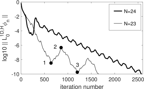
Figure 7: Error evolution of the AITEM (6c) accelerated by ME. Points labeled ‘1’–‘3’ here are not related to points ‘1’, ‘2’ in Fig. 6; they are commented on in Sec. VI.

Figure 7 illustrates two salient points about ME. First, it improves the convergence rate of the AITEM for incommensurate filling fractions even more than for commensurate ones: by over 50 times for $N=24$ and by more than four orders of magnitude for $N=23$. Second, the error evolution of the AITEM with ME can be highly non-monotonic, exhibiting oscillations of some two orders of magnitude (here, for the $N=23$ case). Both types of error evolution, of which the one for $N=24$ was found to be more common, are also the typical scenarios in 2D, as we will discuss in Sec. V.

In order to further improve the convergence rate, it is essential to understand an origin of error oscillations and devise a way to reduce or eliminate them. Especially problematic may seem the large oscillations, where the error first decreases to a value that appears sufficient for practical purposes (e.g., $10^{-8}$ at point ‘1’ in Fig. 7), but then, unexpectedly, increases for several hundred iterations before starting to decrease again. We have been unable to understand the origin of those oscillations; this open problem is to be addressed in future research. We have also tried a number of ad hoc ways to reduce the oscillations, none of which has led to a significant or consistent improvement. These attempts are summarized in the Supplemental Material, so that future researchers would know what has not worked.

One of our attempts, however, led to a novel and non-trivial extension of the ME technique, with the motivation being the following. We mentioned in Sec. III.2 that the ME (20) eliminates not the lowest-$\lambda$ eigenmode of $P^{-1}L$ but rather a mix of several low-$\lambda$ modes that compose (8a). Each of those modes is multiplied by the same $\Gamma_{{\rm slow},n}$, which represents some “average reduction factor” that is designed to reduce the amplitude of an “average” mode. As the analysis in [22] suggests, while the lower-$\lambda$ modes composing (8a) will be suppressed by such an “average reduction factor,” the higher-$\lambda$ modes in (8a) will be amplified by it. This may be a reason leading to an oscillatory evolution of the error. Therefore, one can expect to be able to reduce error oscillations if one eliminates not a single “average mode” (8a) but instead decomposes (8a) into several, “more exact,” eigenmodes and eliminates each of them with its proper reduction factor $\Gamma_{{\rm slow},n}$. This multiple-mode elimination technique is described in the next section.

IV Multiple-mode elimination (mME)

In the first subsection, we will derive equations of the mME, which generalize (20) to the case of multiple modes being eliminated with their individual reduction factors $\Gamma_{{\rm slow},\,n}$. In the second subsection, we will illustrate improvement brought about by this method over the single-mode ME (20) for the 1D Hartree equations (14), as well as discuss certain technical implementation details of both kinds of ME. In the third subsection we will show that both ME techniques are superior to the Anderson Acceleration for the type of problems considered in this work.

IV.1 Derivation of the mME equations

Here we present a conceptual derivation of the method, which culminates in the Algorithm presented towards the end of this subsection. Its implementation issues are discussed in Appendix D.

The main idea is to extract the modes, which will be eliminated later, from increments of the solution at several consecutive iterations. To that end, consider a $K\times(N\cdot M_{x}M_{y})$ matrix that generalizes (8a):

$$\widehat{\Delta}=\left(\begin{array}[]{c}\overrightarrow{\Delta\phi}_{n-1}\\ \vdots\\ \overrightarrow{\Delta\phi}_{n-K}\end{array}\right),$$ (22)

where:  $K$ is the number of modes one plans on eliminating, $M_{x},M_{y}$ are numbers of grid points (see Appendix A), and, by analogy with (6c),

$$\overrightarrow{\Delta\phi}_{n-i}=(\vec{\phi})_{n-i+1}-(\vec{\phi})_{n-i},\qquad i=1,\ldots,K.$$ (23)

Similarly, define another $K\times(N\cdot M_{x}M_{y})$ matrix:

$$L\,\widehat{\Delta}\equiv\left(\begin{array}[]{c}\Delta\big{(}L^{(0)}\vec{\phi}\big{)}_{n-1}\\ \vdots\\ \Delta\big{(}L^{(0)}\vec{\phi}\big{)}_{n-K}\end{array}\right)\,\approx\,\left(\begin{array}[]{c}L\,\overrightarrow{\Delta\phi}_{n-1}\\ \vdots\\ L\,\overrightarrow{\Delta\phi}_{n-K}\end{array}\right),$$ (24)

where

$$\Delta\big{(}L^{(0)}\vec{\phi}\big{)}_{n-i}=L^{(0)}(\vec{\phi})_{n-i+1}-L^{(0)}(\vec{\phi})_{n-i},\qquad i=1,\ldots,K,$$ (25)

and the approximate equality in (24) holds by analogy with (8d). In what follows we will treat this approximate equality as exact; we verified that for $(\vec{\phi})_{n}$ sufficiently close to the exact solution, it holds with high accuracy.

We now assume that each of $\overrightarrow{\Delta\phi}_{n-i}$ is a linear combination of the eigenmodes $\vec{u}_{i},\,i=1,\ldots,K$ of the linearized iteration operator $P^{-1}L$. Inverting, for future convenience, the relation between $\overrightarrow{\Delta\phi}_{n-i}$’s and $\vec{u}_{i}$’s, we write it as:

$$\widehat{U}\equiv\left(\begin{array}[]{c}\vec{u}_{1}\\ \vdots\\ \vec{u}_{K}\end{array}\right)={\bf A}\,\widehat{\Delta}$$ (26)

for some $K\times K$ matrix ${\bf A}$. Eigenmodes of $P^{-1}L$ are to satisfy the relation

$$P^{-1}L\,\widehat{U}\equiv\left(\begin{array}[]{c}P^{-1}L\,\vec{u}_{1}\\ \vdots\\ P^{-1}L\,\vec{u}_{K}\end{array}\right)={{\bm{\alpha}}}\,\widehat{U},$$ (27)

where

$${{\bm{\alpha}}}={\rm diag}\,(\alpha_{1},\ldots,\alpha_{K}).$$ (28)

Entries $\alpha_{i}$ in (28) denote the “average eigenvalue” corresponding to modes $\vec{u}_{i}$. By slight abuse of notations, the subscripts of $\alpha_{i}$ pertain to different modes, whereas previously subscripts of $\alpha_{n}$ pertained to iterations; this is not expected to lead to a confusion. As at the end of Sec. III.2, we stress that eigenmodes $\vec{u}_{i}$ are not the exact eigenfunctions of $L$ but are some mixes of those eigenfunctions, and thus $\alpha_{i}$ are not necessarily $L$’s eigenvalues $\lambda_{i}$, although the former are expected to approximate the latter. More will be said about this in the next subsection. We will continue to refer to the mixes $\vec{u}_{i}$ of the exact eigenfunctions of $P^{-1}L$ as eigenmodes (or modes), thus making a distinction between the modes extracted from $\widehat{\Delta}$ with our procedure described below, on the one hand, and the exact eigenfunctions, on the other hand.

The goal of the subsequent derivation is to find matrix ${\bf A}$; then the modes can be recovered from (26) and $\alpha_{i}$’s can be found from (27).

Following [23, 21] we will work, instead of $P^{-1}L$, with a similar operator $P^{-1/2}LP^{-1/2}$ which, unlike $P^{-1}L$, is Hermitian. Eigenmodes of $P^{-1/2}LP^{-1/2}$ are $P^{1/2}\vec{u}_{i}$, and the latter can be chosen to form an orthonormal set:

$$P^{1/2}\,\widehat{U}\,\big{(}P^{1/2}\,\widehat{U}\big{)}^{T}={\bf I},$$ (29)

where ${\bf I}$ is the $K\times K$ identity matrix. Here and below we use the fact that solutions of our HF equations are real-valued; for the case of complex-valued solution the transposition of a matrix would need to be replaced by Hermitian conjugation. Using (26) and the fact that actions of matrix ${\bf A}$ and operator $P$ commute, one rewrites the last equation as

$${\bf A}\,P^{1/2}\,\widehat{\Delta}\,\big{(}P^{1/2}\,\widehat{\Delta}\big{)}^{T}\,{\bf A}^{T}={\bf I}.$$ (30)

If one writes the Cholesky decomposition of $P^{1/2}\,\widehat{\Delta}\,\big{(}P^{1/2}\,\widehat{\Delta}\big{)}^{T}$ as

$$P^{1/2}\,\widehat{\Delta}\,\big{(}P^{1/2}\,\widehat{\Delta}\big{)}^{T}={\bf C}\,{\bf C}^{T},$$ (31)

where ${\bf C}$ is a $K\times K$ matrix, then the last two equations yield

$$\widetilde{\bf A}\,\widetilde{\bf A}^{T}={\bf I},\qquad\widetilde{\bf A}\equiv\big{(}{\bf A}\,{\bf C}\big{)};$$ (32)

i.e., $\widetilde{\bf A}$ must be an orthogonal matrix.

Next, one acts on both sides of (27) with $P$, multiplies them by $\widehat{U}^{T}$ on the right, and uses (29) and then (26) to obtain:

$${\bf A}\,{\bf B}\,{\bf A}^{T}={{\bm{\alpha}}},\qquad{\bf B}\equiv L\,\widehat{\Delta}\,\widehat{\Delta}^{T}.$$ (33)

Here we have used that actions of ${\bf A}$ and $L$ commute and that

$$P\,\widehat{U}\,\widehat{U}^{T}=P^{1/2}\,\widehat{U}\,\big{(}P^{1/2}\,\widehat{U}\big{)}^{T},$$ (34)

which follows from the facts that the matrix product in (34) is the discrete version of the inner product, as defined in (2), and that $P$ is a Hermitian operator. Using (32), one rewrites (33) as:

$${\bf C}^{-1}\,{\bf B}\,({\bf C}^{-1})^{T}=\widetilde{\bf A}^{T}\,{{\bm{\alpha}}}\,\widetilde{\bf A},$$ (35)

which means that $\widetilde{\bf A}$ is the orthogonal matrix that diagonalizes the Hermitian matrix ${\bf C}^{-1}\,{\bf B}\,({\bf C}^{-1})^{T}$. The Hermitian character of the latter matrix follows from that of ${\bf B}$, which, in turn, amounts to the equality

$$L\,\overrightarrow{\Delta\phi}_{i}\;\overrightarrow{\Delta\phi}_{j}^{T}=L\,\overrightarrow{\Delta\phi}_{j}\;\overrightarrow{\Delta\phi}_{i}^{T}.$$ (36)

This last relation follows from the fact that the inner products there are the discrete approximations of the continuous inner product defined in (2) and that $L$ is a Hermitian operator in the space of functions satisfying the linearized constraints (2) [23, 21]. Indeed, $\overrightarrow{\Delta\phi}_{i}=\tilde{\phi}_{n-i+1}-\tilde{\phi}_{n-i}$ (see (9)) satisfy those linearized constraints by virtue of individual $\tilde{\phi}_{n-i}$’s satisfying them (when the iterated solution is sufficiently close to the exact one). This issue is further commented on in Appendix D.1.

The above derivation leads to the following Algorithm of mME.

1. Compute the matrix on the l.h.s. of (31) and find its Cholesky decomposition, given by the r.h.s. of that equation.

2. Compute matrix ${\bf B}$ as defined in (33); then find the diagonalization of the matrix on the l.h.s. of (35). This gives one matrices ${{\bm{\alpha}}}$ and $\widetilde{\bf A}$ and then, via (32), ${\bf A}$.

3. Modes $\vec{u}_{i}$ (or $P^{1/2}\vec{u}_{i}$) are then computed via (26). The corresponding $\alpha_{i}$ have already been computed at the previous step.

4. For each mode $i$ we compute its individual $\gamma_{{\rm slow},\,i}$ via (8b) that uses $\alpha_{i}$ computed at Step 2. (Note that the subscript refers to the mode, not iteration, number.) Then compute $\Gamma_{{\rm slow},\,i}$ by (20a), where $\overrightarrow{u_{\rm slow}}$ is replaced by the respective $\vec{u}_{i}$.

5. Finally, the entire $\Gamma$-term in (6a) is replaced by the sum of all $\Gamma_{{\rm slow},\,i}\,$-terms.

IV.2 Performance of mME in 1D

Here we will discuss how mME performs relative to the single-mode ME for the same two cases that were considered in Sec. III.3. Through extensive experimentation, we have found these results to be typical. At the end we will address some of the implementation details of both kinds of ME; other details are found in Appendix D. Simulation parameters were the same as those used in Secs. III.2 and III.3.

For the case of $N=23$ atoms in 30 minima of $V_{\rm ext}$, we did not observe any consistent or significant benefit of eliminating multiple modes versus a single one, for any values of $s$ in the range $[0.1,\,0.8]$. In fact, in most of our attempts, an increase of the number of eliminated modes led to an increase in the number of iterations. We conclude, therefore, that the large error oscillations seen in Fig. 7 must be related to factors other than the presence of multiple slow modes.

Results for the other case, with $N=24$ helium atoms, are shown in Table 1. These results show that increasing the number $K$ of eliminated modes does, on average, tend to decrease the number of iterations. However, since both the computational time and computer memory usage increase with $K$, one should focus on the minimum $K$ value that still provides a sizable reduction of the iteration count. Such a value appears to be $K=3$ or $4$. This observation will guide our choice of $K$ in 2D simulations, presented in Sec. V, where the computational cost of experimentation with mME’s adjustable parameters in more prohibitive than that in 1D.

	1	2	3	4	5	6	7
0.05	1500	1200	1500	1100	1400	1400	1200
0.1	2700	1400	1700	1500	1200	1300	1000
0.2	4500	1600	1100	1000	1200	1300	1000
0.4	5600	1500	1400	1300	1300	1200	1100

Table 1: Number of iterations (rounded to the nearest hundred) required for the error to decrease to $10^{-10}$, versus the number of eliminated modes $K$ and parameter $s$, for $N=24$ helium atoms in $V_{\rm ext}$ (15) with 30 minima. Other adjustable parameters of (m)ME are as stated at the end of this subsection.

For completeness and comparison with the results reported in the next subsection, we mention that increasing $K$ past seven does not consistently reduce the number of iterations, which stays around 1000 up to $K=15$, the largest number that we tested. Yet, increasing $K$ did improve the convergence rate when the error got sufficiently small. What made the total number of iterations not decrease with the increase of $K$ was that the duration of the transient — i.e., when the error would not decay overall, as between iterations 100 and $\sim 300$ in Fig. 7 for $N=24$, — tended, on average, to be longer for a greater $K$. In principle, this would open up the possibility of reducing the total number of iterations by using a smaller $K$ at the beginning — for a shorter transient — and a grater $K$ later — for a faster convergence rate, — but we did not explore this further as our focus was not on fine-tuning the performance of the mME.

Now, we again emphasize that the eliminated modes $\vec{u}_{i}$ are not the exact eigenfunctions of the linearized iteration operator $P^{-1}L$ and, thus, the corresponding $\alpha_{i}$ are not the exact eigenvalues of $P^{-1}L$. The composition of the eliminated modes in terms of the eigenfunctions appears to depend on the number $K$ of the modes that one sets to eliminate, and, hence, so do the “dynamic average eigenvalues” $\alpha_{i}$. This is illustrated in Fig. 8(a,b), where one notices that $\alpha_{i}$ depend on the value of $K$ chosen (and, of course, they vary from one iteration to the next). Incidentally, the minimum computed values of $\alpha_{1}$ are seen to agree, by the order of magnitude, with the estimates of $(\lambda_{P^{-1}L})_{\min}$ presented in Appendix C.2 for both $N=24$ and $N=23$ cases.

We conclude this subsection with two remarks about implementation of the ME. The first remark pertains to both single- and multiple-mode ME. Parameter(s) $\alpha_{n}$ ($(\alpha_{i})_{n}$) found by the code at some iterations can be quite small and even negative. The former (i.e., $\alpha_{n}$ being “too small”) would make $\gamma_{n}$, computed by (8b), very large. While the corresponding $\Gamma$-term will reduce the specific mode of the iterated solution, as intended, it may amplify other modes (unintentionally), thereby impeding the convergence. Similarly, having $\alpha_{n}<0$ would make $\gamma_{n}>0$, and this can also impede convergence via the same mechanism. To prevent this from occurring, we imposed the condition:

$$-10^{7}\leq\gamma_{n}\leq 0,$$ (37)

where the lower bound was found to be overall optimal across many tens of tested cases in both 1D and 2D.

The second remark is specific to the mME. As mentioned earlier, the memory requirements increase with $K$, the number of modes one needs to store. Yet, Fig. 8 shows that only few of the $\alpha_{i}$’s can be as low as $O(10^{-2})$ or lower, which per (12) would make the corresponding modes to converge in as many as several thousand iterations. Such modes indeed need to be eliminated by the ME. However, most other $\alpha_{i}$’s are at least an order of magnitude greater and the corresponding modes would decay to the required tolerance of $10^{-10}$ “on their own,” i.e., without being eliminated by the $\Gamma$-term, in only a few hundred, or fewer, iterations. Therefore, to save computational resources, we first computed $\alpha_{i}$’s as eigenvalues of the l.h.s. of (35) but then computed and eliminated only the modes with

$$\alpha_{i}<\alpha_{\max}.$$ (38)

For the results presented in this subsection, we used $\alpha_{\max}=0.2$.

It is important to clarify that while only few $\alpha_{i}$’s (usually, no more than four) “go” below $\alpha_{\max}$, increasing $K$ still may improve the convergence rate, as evidenced by Table 1. This is because the allowing for more modes “pushes” the smaller of their eigenvalues down (compare Figs. 8(a) and 8(b)), thereby making more of them satisfy (38).

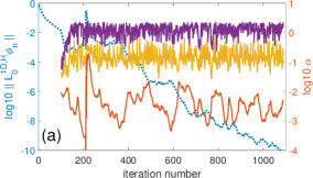
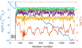
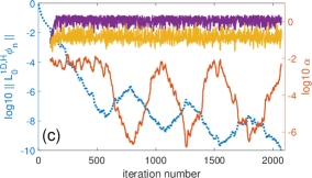
Figure 8: Evolutions of the error (blue dotted line, left axis) and $\alpha_{i}$’s, $i=1,\ldots,K$, computed from (35) (solid lines, right axis) for the cases considered in Sec. III.3. Panels (a) and (b): $N=24$; panel (c): $N=23$. Numbers of eliminated modes are: $K=3$ (a,c) and $K=5$ (b). In all panels, $s=0.2$. Note that the right axis in (c) has a different scale than that in (a,b).

IV.3 Comparison of ME with Anderson Acceleration (AA)

Figure 9 demonstrates that in those cases where the ME accelerates the AITEM so that it converges in one to two thousand of iterations, the AITEM with the well-known AA [14] performs considerably worse. The AA does not eliminate modes, but instead uses the solution at $K_{AA}$ previous iterations to subtract their certain combination to minimize the error. The values of $K_{AA}\leq 5$ are shown in the legend of panels (a,b). For those lower $K_{AA}$, the best result achieved by the AA is about twice as slow as that achieved by the mME (for $N=24$; refer to Sec. IV.2 regarding $N=23$), and for more previous iterations/eliminated modes (namely, five) than the best results shown in Table 1. The benefit of the AA with $K_{AA}\geq 12$ becomes comparable to that brought about by the mME with $K$ as low as 3: compare Fig. 9(c) with Table 1. While the memory requirements associated with a larger number of previous iterations stored is not an issue in 1D, it becomes significant in 2D. Thus, due to this inferior overall performance by the AA relative to the mME, we will not use the former for the 2D simulations reported in the next section.

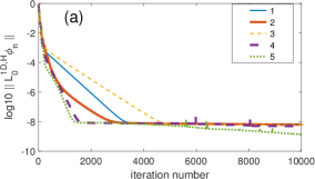
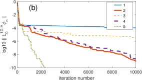
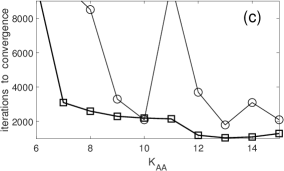
Figure 9: (a,b):  Error evolution of the AITEM (with $\Delta t=0.6$ and $c=100$ in $P$) with the Anderson Acceleration for the two cases considered in Secs. III.3, IV.3: $N=23$ (a) and $N=24$ (b). See main text for more details.  (c): Number of iterations to convergence to $10^{-10}$ versus the number of previous iterations (up to 15) whose information is used by the Anderson Acceleration: $N=23$ (circles) and $N=24$ (squares); the lines are guides to the eye. Numbers of iterations greater than 9000 indicate that convergence was not achieved in 10,000 iterations.

V 2D patterns obtained with AITEM

Here we will compare the performance of mME and the original single-mode ME (sME) for several representative 2D periodic patterns that helium atoms can form over graphene. The equations simulated are those presented in Sec. II.1. The common parameters for all simulations are:  $\Delta t=0.4$; $E_{\rm clip}=2000$K leading to $c=200$ in (7); ME starts at the 100th iteration; conditions (37) and (38) were imposed, with $\alpha_{\max}=0.1$. The values $s$ and $K$ which we used in this section were motivated by the results of Sec. IV.2.

As in Sec. IV.2, there were patterns (i.e., values of $f\!f$) for which mME performed, on average, better than sME, and those for which it did not. The results for the former group are shown in Table 2. The equilibrium pattern for $f\!f=1/2$ is depicted in Fig. 10; the patterns for $f\!f=7/16$ and $7/12$ can be found in the literature and therefore are shown in Supplemental Material. Initial placement of helium atoms was done by the Second Initial placement procedure (Appendix A.3) for all filling fractions except $f\!f=1/2$ (and $f\!f=2/3$ mentioned below), where that procedure led to non-periodic patterns in a large percentage of random initial placement; therefore, for $f\!f=1/2$ ((and for $f\!f=2/3$) we used the First procedure. The simulation window consisted of $8\times 8$, $8\times 4$, and $12\times 4$ rectangular periods for $f\!f=7/16,\,1/2$, and $7/12$, respectively; recall (Sec. II.3) that one such a period contains two minima of $V_{\rm ext}$. For each pair ($f\!f$, $s$), Table 2 shows the number of iterations for six different initial conditions for the placement of helium atoms, with the same condition being used to obtain results for the sME ($K=1$) and mME ($K=3$). While this number of initial conditions is not statistically significant, we have observed qualitatively similar performance of the mME relative to the sME in many exploratory simulations not reported here.

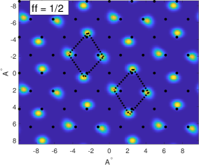
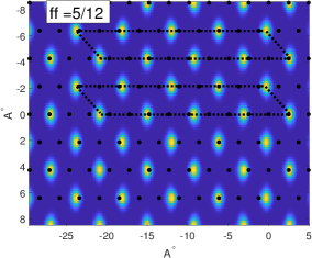
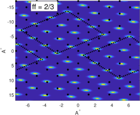
Figure 10: Equilibrium particle densities, i.e., $\sum_{j=1}^{N}|\phi_{j}|^{2}$, for some of the filling fractions reported in this section. Darkest blue in each panel corresponds to zero, while brightest yellowish, to the maximum density. Black dots denote the locations of centers of graphene hexagons (i.e., minima of $V_{\rm ext}$). Dotted lines show two periods of the pattern. The reverse direction/labels of the vertical axis are an artefact of Matlab’s command imagesc.

	$f\!f=7/16$			$f\!f=1/2$			$f\!f=7/12$
	$\quad s=0.05\quad$	$s=0.1\quad$	$s=0.2\quad$	$\quad s=0.05\quad$	$s=0.1\quad$	$s=0.2\quad$	$\quad s=0.05\quad$	$s=0.1\quad$	$s=0.2\quad$
$\;K=1$	3300	3800	4300	2400	3300	4400	4600	4600	4000
$K=3$	3200	3600	3700	1600	1600	1800	3300	3100	3000
ratio	0.97	0.95	0.86	0.67	0.48	0.41	0.72	0.67	0.67
$K=1$	2200	3100	4700	2500	3400	4300	2800	3000	2700
$K=3$	2100	1900	4200	1600	1600	1500	2100	3600	2900
ratio	0.95	0.61	0.89	0.64	0.47	0.35	0.75	1.2	1.1
$K=1$	3600	4200	4800	2000	2000	2300	2200	12800	4100
$K=3$	2500	3100	3000	1500	1600	1600	4600	2700	2400
ratio	0.69	0.74	0.63	0.75	0.80	0.70	2.1	0.21	0.68
$K=1$	3500	4000	4000	2100	2700	3100	3400	9200	7100
$K=3$	2600	2800	2400	1500	1600	1800	2600	2300	2700
ratio	0.74	0.70	0.60	0.71	0.59	0.58	0.76	0.25	0.38
$K=1$	2800	3700	3900	2200	2300	2300	2300	2200	2600
$K=3$	2100	2200	2900	1700	1700	1900	2500	2400	2600
ratio	0.75	0.59	0.74	0.77	0.74	0.83	1.1	1.1	1.0
$K=1$	3100	3800	4400	1700	1800	1800	2600	3100	3900
$K=3$	3000	2300	2300	1300	1500	1400	2500	2500	2600
ratio	0.97	0.61	0.52	0.76	0.83	0.78	0.96	0.81	0.67

Table 2: Number of iterations (rounded to the nearest hundred) required for the error to decrease to $10^{-10}$ for three different periodic patterns, as obtained with sME ($K=1$) and mME ($K=3$). A triplet of vertically aligned numbers enclosed between two horizontal lines corresponds to one random realization of the initial condition (see Appendix A.3); thus, for each $f\!f$, the Table presents results for six random initial conditions for each $s$ value. Within the same set of horizontal lines, the initial conditions are different for different $f\!f$ (naturally) and may be different for the same $f\!f$ and different $s$. The latter is because some initial conditions could converge to non-periodic patterns for some of the values of $s$. The ratios in the third line of each row are those of the two numbers directly above, shown for ease of comparison of performances of sME and mME.

This performance can be summarized as follows: While the mME is not guaranteed to always reduce the number of iterations, it does so on average by about 30%. Perhaps more importantly, the use of the mME leads to a more narrow range for the iteration numbers across different initial conditions than the sME. Also, for any $f\!f$, using $s=0.05$ leads, again on average, to fewer iterations than the larger values of $s$.

On the other hand, for $f\!f=5/12$ and $2/3$, whose equilibrium patterns are shown in Fig. 10, we found that mME does not reduce the number of iterations and may even, on average, increase it compared to the sME. This is analogous to the case $N=23$ considered in Sec. IV.2. Just as there, we found that a hallmark of this case is the high oscillations of the error, as in Fig. 8(c). In contrast, for the cases where the mME helped to reduce the number of iterations, the error oscillations were much smaller, similarly to those in Figs. 8(a,b). The evolution of $\alpha_{i}$ in 2D were found to also be similar to the respective cases shown in Fig. 8. For completeness, we note that the simulation window consisted of $24\times 4$ and $6\times 8$ rectangular periods for $f\!f=5/12$ and $2/3$, respectively.

VI Conclusions and Discussion

In this paper we have presented the details of an Accelerated Imaginary Time Evolution Method (AITEM) for Hartree–Fock (HF) equations. Its essential steps are given in (6c) with the $\Gamma$-term (for a single eliminated mode) given by (20). The optimal value of parameter $c$ in the preconditioner (7) is given by relation (17), with $E_{\rm clip}$ defined in Appendix A.1. We stress that this relation is expected to hold for any hard-core-type (i.e., strongly repulsive at short distances) potentials, which will need to be clipped when implemented in an ITEM or another relaxation-type method. Other implementation details of the AITEM (6c) are found in Appendices A.1 and A.2, and initial placement of atoms being simulated is discussed in Appendix A.3. The mode-elimination (ME) step of the AITEM, discussed in Secs. III and IV, is shown to consistently improve convergence of the optimally preconditioned ITEM by at least an order of magnitude, and often by much more. Values of the ME parameter $s$, which controls the amount of modes that are being eliminated, are discussed in Secs. III.2 and IV.2. For HF equations, we found optimal $s$ values to be significantly lower than those found in earlier studies for just one or two equations (which also did not have hard-core-type potentials).

The developments listed in the previous paragraph pertain to optimizing the form of the AITEM, which was proposed in earlier studies. This work also presents a novel method to accelerate the AITEM: the multiple-mode elimination (mME). Its derivation and Algorithm are found in Sec. IV.1, and implementation details are discussed at the end of Sec. IV.2 and in Appendix D. As we demonstrate in Secs. IV.2 and V, the mME even with a small number $K$ of eliminated modes provides an improvement of around 30% (on average) over the single-mode elimination (sME) in those cases where the iteration error obtained by the sME fluctuates moderately (see the thick line in Fig. 7). There, the mME also makes the number of iterations required for convergence slightly less dependent on the initial conditions and on values of parameter $s$. We also found that when, on the contrary, error oscillations in the AITEM with sME are large, as illustrated by the thin line in Fig. 7 (see also the discussion at the end of Sec. III.3), the mME does not further improve convergence.

Understanding the mechanism behind error oscillations remains an open problem. In the Supplemental Material we listed several approaches that we tried to reduce or remove them. Here we present an argument that even if a “cure” for those oscillations is not found in the future, the problem of waiting for the iterations to converge to a prescribed low tolerance can be circumvented. This argument is based on two facts:

• The reason for setting a low tolerance for convergence is not that such accuracy of solutions is needed in practice. Rather, it is merely to be assured that the iterations would eventually reach a (local) minimum of the energy landscape rather than a saddle point. (In the latter case, the iterations would eventually diverge after converging initially; this is the type of the behavior seen at points 1 and 3 in Fig. 7.)

• By comparing solutions obtained at points 1–3 in Fig. 7 with the final solution, we observed that $\left\|\vec{\phi}_{\rm pt}-\vec{\phi}_{\rm final}\right\|$ decreases monotonically when ‘pt’ increases from 1 to 2 to 3. That is, even though the error of the equations does not decrease monotonically, the error of the solution does. (This is similar to the discussion about Fig. 6 found in Sec. III.3 about the AITEM without ME.)

Therefore, a meaningful way to stop iteration in a case where the equation error has large oscillations could be when one observes that the error begins to grow the second time, as at point 3 in Fig. 7. Indeed, by waiting past that point one would obtain a slightly more accurate solution, but this will be achieved at the expense of several hundred more iterations.

Both single- and multiple-mode versions of ME were shown, in Sec. IV.3, to perform significantly better than the well-known Anderson Acceleration. From a philosophical perspective, this result may appear not surprising given that the ME uses (and requires) more information of the iteration operator — namely, its Hermitianness, — than the AA, which would work for any iteration operator.

We believe that the acceleration techniques proposed in this work for the ITEM will also be useful for other iteration methods.

As a byproduct, our 2D simulations revealed three interesting periodic patterns that helium atoms can form over graphene (or graphite): $f\!f=5/12$, $1/2$, and $2/3$ (surface coverages of 0.0796, 0.0955, and 0.127 Å^-2, respectively); see Sec. V. As explained in Sec. II.3, the latter pattern can form only in a 2D system, or in 3D when the motion of helium atoms in the direction perpendicular to graphene’s surface is prohibited/restricted. The periodicity of the patterns was verified by taking their 2D Fourier transform. We acknowledge that a periodic pattern for $f\!f=31/75\approx 0.4133$, which is very close to $f\!f=5/12\approx 0.4167$, was mentioned in Refs. [31, 32], but no picture of it was provided. Also, a phase with $f\!f=13/24\approx 1/2$ was shown in Fig. 5(c) of Ref. [29]; it appears similar to the $f\!f=1/2$ pattern shown in our Fig. 10, but was termed ‘incommensurate’ in [29].

Finally, we comment on some extensions of our method and future research. In general, the AITEM developed in this work can be used to simulate hard-core bosons and fermions in various settings. For example, it can be used to compute the nearest- and next-nearest-neighbor interaction strength in a variety of lattice Bose–Hubbard models (see, e.g., [33, 34, 35, 36]), as two of the present authors did in Ref. [9], which motivated this research. The same method can also be used to study distribution of atoms (helium and others), including their forming various periodic patterns over surfaces periodic at the atomic level [37, 38, 39, 40].

When spatial orientation of the adsorbed atom or molecule is essential (as, e.g., in [40]), the method would need to be extended to include the rotational degrees of freedom in the Hamiltonian and the third spatial dimension, while using the same underlying concepts. A 3D extension of the method can also be used to study formation of a small number of layers of adsorbed atoms over surfaces [28].

Simulations of the full $N$-body wavefunction by ab initio methods such as path integral quantum Monte Carlo produce more physically accurate results for adsorbed phases of atoms than simulations of the HF equations. However, the latter simulations by the numerical method presented in this work are substantially less computationally costly. Therefore, the AITEM could be a useful tool in high-throughput schemes [41] that would employ HF equations to identify promising scenarios for realizing exotic low-dimensional adsorbed superfluid phases. This may include searching for optimal materials as substrates or for optimal tunable parameters of known substrates, as, e.g., in [42].

Appendix A:  DFT for evaluation of terms in (4) and for initial placement of helium atoms

We use Discrete Fourier transform (DFT) and its inverse defined as:

$$\sum_{\bf{n}=\bf{0}}^{\bf{\max}}e^{-i\,{{\bf r}}_{\bf{n}}\cdot\bf{k}_{\bf{m}}}\,\phi_{\bf{n}}\equiv F[\phi]_{\bf{m}},\qquad\phi_{\bf{n}}=\frac{1}{M_{x}M_{y}}\sum_{\bf{m}=\bf{0}}^{\bf{\max}}e^{i\,{{\bf r}}_{\bf{n}}\cdot\bf{k}_{\bf{m}}}\,F[\phi]_{\bf{m}}\equiv F^{-1}\left[\,F[\phi]\,\right]_{\bf{n}},$$ (39)

where: $M_{x},M_{y}$ are the numbers of grid points along $x$ and $y$; all vectors have two components pertaining to $x$ and $y$, e.g.,: ${\bf n}=(n_{x},n_{y})$, ${{\bf r}}_{\bf{n}}=(x_{n_{x}},y_{n_{y}})$, ${\bf\max}=(M_{x}-1,M_{y}-1)$, ${\bf k}_{\bf{m}}=\big{(}(k_{x})_{m_{x}},(k_{y})_{m_{y}}\big{)}$, etc. Here $x_{n_{x}}=(n_{x}-1)\Delta x$, $(k_{x})_{m_{x}}=(m_{x}-1)\Delta k_{x}$, etc., where $\Delta x$ and $\Delta k_{x}$ are the respective mesh sizes. Note that in this Appendix, $\bf{n}$ refers to the index of grid points in the physical space, while in the main text $n$ referred to the iteration number.

The Laplacian in (4) is computed in the standard way:

$$-\nabla^{2}\phi=F^{-1}\big{[}\,\|({\bf k})_{\rm shifted}\|^{2}\,F[\phi]\,\big{]},$$ (40)

where $\|\ldots\|$ stands for the Euclidean norm,

$$\big{(}(k_{x})_{\rm shifted}\big{)}_{m_{x}}=\left\{\begin{array}[]{ll}(k_{x})_{m_{x}},&m_{x}\in[0,\,M_{x}/2-1];\\ -(k_{x})_{M_{x}-m_{x}},&m_{x}\in[M_{x}/2,\,M_{x}-1],\end{array}\right.$$ (41)

and similarly for $(k_{y})_{\rm shifted}$.

A.1: Computing the nonlocal term in (4)

In this paragraph, we treat the case of one spatial dimension for the sake of clarity; its 2D generalization will be given later. We begin by setting up $V_{\rm int}$ to be periodic on the computational grid and also clip it removing the “singularity” at ${{\bf r}}=\bf{0}$ at some empirically chosen value

$$E_{\rm clip}\gg 1,$$ (42)

as illustrated in Fig. 11. Note that, given the definition of $x_{n_{x}}$ above, array $V_{\rm int}(x_{n_{x}})$ is defined so as to reflect the fact that the interaction is the strongest at zero separation between helium atoms. With this setup, for any function $\psi({{\bf r}}^{\prime})$, one has:

$$\int V_{\rm int}({{\bf r}}-{{\bf r}}^{\prime})\,\psi({{\bf r}}^{\prime})\,d{{\bf r}}^{\prime}=F^{-1}\left[\,F[V_{\rm int}]\,F[\psi]\,\right].$$ (43)

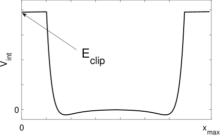
Figure 11: Schematics of the interaction potential between helium atoms, set up as explained before Eq. (43). Details along the $x$-axis are not to scale: the attracting “tail” past the minimum of $V_{\rm int}$ at $x\approx 3$Å actually extends much longer towards $x_{\max}/2$.

We verified that a derivative discontinuity introduced by the clipping of $V_{\rm int}$ does not appear to introduce numerical artifacts in $F[V_{\rm int}]$. This is because the very high gradient of this potential at sufficiently small distances already produces a long “tail” in its Fourier spectrum.

The code snippet below shows how $V_{\rm int}$, originally defined in [20] as a 1D array over a 1D vector rint, is interpolated on a 2D grid in Matlab:

[X,Y] = meshgrid(x,y); % create 2D grid along x and y
rint_arr = sqrt(X.^2 + Y.^2); % distance from center of grid
rint_vec = reshape(rint_arr,[1,M_x*M_y]); % make it 1 x (Mx*My) vector
Vint_vec = interp1(rint,Vint,rint_vec); % interpolate Vint from rint to rint_vec
Vint_arr = reshape(Vint_vec,[Mx,My]); % put it over Mx x My grid

The resulting 2D array Vint_arr peaks at the center of the numerical grid and decays towards its boundaries, which is not how $V_{\rm int}$ is set up in Fig. 11 and upon which assumption Eq. (43) is written. To adjust for this difference, an fftshift command must be placed either around the entire r.h.s. of that equation or around the $F[V_{\rm int}]$ term.

We now show how all the $N(N+1)/2$ Hartree terms in Eqs. (4) can be computed in $O(N)$ steps:

• Compute $F[\phi_{i}^{2}]$ for all $i$ and then define $F[S]\equiv\sum_{i=1}^{N}F[\phi_{i}^{2}]$.

• Use (43) with $\psi=S-\phi_{j}^{2}$ to compute the Hartree sum in (4) for each $j$.

A.2: Verifying validity of clipping $V_{\rm int}$

The clipping here refers to the procedure mentioned before Eq. (42). Specifically, we need to verify that a somewhat arbitrarily chosen value $E_{\rm clip}$, which we took to be $E_{\rm clip}=1000$ K and $2000$ K for 1D and 2D simulations, respectively, does not significantly alter the simulation results. (For the original $V_{\rm int}$ from [20], $(V_{\rm int})_{\rm not\;clipped}(0)\approx 2\cdot 10^{6}$ K.) To that end, one can monitor the difference between quantities

$$(E_{{\rm int},\,j})_{\rm clipped}=\langle\,\sum_{i=1,\,i\neq j}^{N}\phi^{2}_{i}|(V_{\rm int})_{\rm clipped}|\phi^{2}_{j}\,\rangle\quad{\rm and}\quad(E_{{\rm int},\,j})_{\rm not\;clipped}=\langle\,\sum_{i=1,\,i\neq j}^{N}\phi^{2}_{i}|(V_{\rm int})_{\rm not\;clipped}|\phi^{2}_{j}\,\rangle\,,$$ (44)

and check whether it exceeds a specified amount (see below), for all atoms $j$. Here all the solutions $\phi_{i}$ in (44) are computed with $(V_{\rm int})_{\rm clipped}$. Choosing $E_{\rm clip}$ too low, obviously, increases the difference in (44). On the other hand, choosing $E_{\rm clip}$ too high leads to the need to decrease $\Delta t$ so as to avoid extreme sensitivity of the solution, whereby tiny changes of $\phi_{i}$ or $\phi_{j}$ at the locations of its neighbors would lead to very large and unphysical changes in the entire system (examine the first term in $[\cdots]$ in (6a)). In turn, too small a $\Delta t$ slows down convergence of the iterations.

Now, since the simulated equations (6c) “do not know” that the true helium–helium interaction potential is $(V_{\rm int})_{\rm not\;clipped}$ rather than $(V_{\rm int})_{\rm clipped}$, they have no way of correcting a discrepancy between the two quantities in (44) if such arises. Such a discrepancy did occur in many of our simulations and was due, usually, to $\phi_{j}$ “developing too big of a piece” (usually, of a size less than 1% of its peak value) at the location of one of its neighbors. An external correcting procedure was needed when that occurred. Through extensive testing, we found the following one to work.

Procedure for bounding  $\delta E_{j}=|(E_{{\rm int},\,j})_{\rm clipped}-(E_{{\rm int},\,j})_{\rm not\;clipped}|$

• Compute $\delta E_{j}$ every $n_{\rm monitor}$ iterations. We used $n_{\rm monitor}=200$. Doing so too often will slow down the code, while doing so too infrequently may extend a transient period which is required for helium atoms move sufficiently close to their equilibrium locations.
  Find those $j$ for which $\delta E_{j}$ exceeds some threshold. We used the criterion  $\delta E_{j}>5\cdot\min_{j}\delta E_{j}$, which amounted to roughly 1K.

• Estimate the width of any one helium atom whose $\delta E_{j}$ is below the threshold. Replace (see (45) below) those $\phi_{j}$ whose $\delta E_{j}$ exceeds the threshold with a Gaussian of the above width. (As a simpler alternative, which may slightly increase the length of the calculations, use the initial Gaussian guess.)

• Apply the Gram–Schmidt orthogonalization to enforce conditions (2).

A.3: Initial placement of helium atoms

We first outline the two procedures that can be used to create an initial filling fraction $p/q$ of helium atoms and then how they were implemented using DFT.

First initial placement procedure:  We first distributed $2(p/q)\,N_{{\rm cells},\;x}$ atoms over two consecutive rows of cells, placing them equidistantly along each row and horizontally shifting atoms in the second row relative to those in the previous row so as to maximize the distance between any two atoms in the two rows. We then added to coordinates of each atom a random perturbation of size $\sim 20\%$ of the cell’s side (i.e., of $d_{0}/\sqrt{3}$).

Second initial placement procedure:   We first found integer factors $N_{{\rm He},\;x}$ and $N_{{\rm He},\;y}$ of the total number of helium atoms $N$; the code does so by going through various combinations of these factors starting with an initial guess $N_{{\rm He},\;x}=\sqrt{f\!f}\,N_{{\rm cells},\;x}$ rounded to the nearest integer. Since, as mentioned in Sec. II.3, $N_{{\rm cells},\;y}$ must be even, so must be the selected factor $N_{{\rm He},\;y}$. Second, we placed the atoms so that any two consecutive atoms within one row (i.e., along $x$) are $\delta_{{\rm He},\;x}=(M_{x}/N_{{\rm He},\;x})\Delta x$ apart, with the rows being spaced by $\delta_{{\rm He},\;y}=(M_{y}/N_{{\rm He},\;y})\Delta y$ along $y$. Any two consecutive rows of atoms are shifted horizontally by $\delta_{{\rm He},\;x}/2$ so as to maximize the distance between any two atoms, as in the first placement procedure. Finally, to those locations we add random perturbations of the size of $\sim 20\%$ of $(\delta_{{\rm He},\;x}-d_{0})/2$ and $(\delta_{{\rm He},\;y}-d_{0})/2$ along the $x$- and $y$-directions, respectively.

Of these two procedures, the second one usually yields a more uniform initial placement for smaller $ff$.

Finally, the implementation of the initial placement of helium atoms at specified locations $\vec{{\bf r}}_{c}\equiv(x_{c},y_{c})$ of the lattice is straightforward with (39). Namely, one first creates a localized (typically, Gaussian) function $\phi_{0}({\bf r})$ centered at ${\bf r}=0$ and then shifts it to the desired location via:

$$\phi({\bf r}-{\bf r}_{c})=F^{-1}\left[F[\phi_{0}]\,e^{-i\,{\bf r}_{c}\cdot\bf{k}}\,\right].$$ (45)

Appendix B:  Discussion of the $V_{\rm int}$-term in Sec. III.1

For the purpose of the estimate in (16) and the text below it,

$$\mbox{`$V_{\rm int}$-term'}\equiv\left\|\sum_{i\neq j}\langle\phi_{i}|V_{\rm int}|\phi_{i}\rangle\,f_{j}+2\sum_{i\neq j}\langle\phi_{i}|V_{\rm int}|f_{i}\rangle\,\phi_{j}\,\right\|\,/\,\|\vec{f}\|,$$ (46)

where $f_{j}$ is the component of eigenfunction $\vec{f}$ of $P^{-1}L$ corresponding to helium atom $j$. Our goal here is to show that it is feasible that this term can be $O(E_{\rm clip})$ for some of the eigenfunctions, even though it may not be obvious at first sight.

Both terms in the numerator above depend on the overlap between $\phi_{i}$ and $f_{j}$ for $i\neq j$. Note that the magnitude of neither term can be inferred from the $V_{\rm int}$-term in the original, non-linearized equation, (3) or (14), i.e., from $\left\|\sum_{i\neq j}\langle\phi_{i}|V_{\rm int}|\phi_{i}\rangle\,\phi_{j}\,\right\|$. The latter term is on the order of $V_{\rm int}(d)$, where $d$ is the distance between neighboring helium atoms. When $d=d_{0}$, the distance between centers of adjacent graphene cells, $O(V_{\rm int}(d_{0}))=10\ldots 100$ K $\ll E_{\rm clip}$ [9]. (For $d>d_{0}$, $V_{\rm int}(d)$ is even smaller.) This occurs because the overlap between (the wavefunctions of) helium atoms even in adjacent wells of $V_{\rm ext}$, i.e., $\langle\phi_{i}|\phi_{j}\rangle$, $i\neq j$, is quite small.

However, for certain eigenfunctions of $P^{-1}L$, the overlap $\phi_{i}$ and $f_{j}$, $i\neq j$, can be much greater than that between helium atoms in the adjacent wells of $V_{\rm ext}$. This is illustrated in Fig. 12. Due to this greater overlap, the size of the $V_{\rm int}$-term as defined in (46) is much greater than $O(V_{\rm int}(d_{0}))$. In fact, from the estimate (17) extrapolated to $k=O(1)$ and the fact that using $c=E_{\rm clip}$ yields $max(\lambda)=O(1)$ in this case, one can infer that the $V_{\rm int}$-term for these eigenfunctions is $O(E_{\rm clip})$.

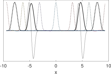
Figure 12: Eigenfunctions of $P^{-1}L$ with $c=E_{\rm clip}=100$ for $N=6$ helium atoms placed in $N$ adjacent wells of $V_{\rm ext}$, corresponding to some of its largest eigenvalues: $\lambda=1.777=\lambda_{\max}$ (thick solid), $\lambda=1.772$ (thick dotted), $\lambda=1.702$ (thin solid). Thin dashed lines show the locations of the helium atoms. Vertical scale is in arbitrary units.

Appendix C:  On the lowest eigenvalue of of $P^{-1}L$ and its eigenfunction

C.1:  The lowest-$\lambda$ eigenfunction corresponds to a common shift of all atoms

In this subsection, we will justify its title. Suppose that $V_{\rm ext}\equiv 0$. Then any periodic array of atoms can be shifted as a whole without changing its energy. In this case, the common shift mode has $\lambda=0$. Other modes that involve unequal shifts or breathing of atoms would increase the total energy via the term $\langle\phi_{i}\,|V_{\rm int}|\,\phi_{j}\rangle$, due to the rapidly-increasing repulsion between the atoms with their decreasing separation. Therefore, such modes will have $\lambda>0$. Now, when $V_{\rm ext}\,\cancel{\equiv}\,0$, a common shift of all atoms would raise the array’s energy due to the atoms shifting away from $V_{\rm ext}$’s minima; hence the eigenvalue of that mode becomes positive. The reason that it is small is that the change in the external potential energy due to such a shift is still much smaller than a change that would occur had the distance between adjacent atoms changed. In other words, $V_{\rm ext}$ acts as a small perturbation in a system where the total potential energy is dominated by $V_{\rm int}$.

For the commensurate filling fraction $f\!f=1/2$ the low-$\lambda$ part of the spectrum of $P^{-1}L$ looks quite different than that for $f\!f=1$, shown in Fig. 5. For the same parameters as used in Fig. 5 except that now $N=3$, the common shift mode is still the lowest with $\lambda_{\min}=0.020$; however, that value is considerably greater than $\lambda_{\min}=0.0053$ for $f\!f=1$. This explains the faster convergence of the AITEM without ME for $f\!f=1/2$ (given that $\lambda_{\max}\approx 1$), as noted at the end of Sec. III.2. Moreover, the next few modes have eigenvalues that are much closer to $\lambda_{\min}$ than in the $f\!f=1$ case: $\lambda_{=}0.023,\,0.034,\,0.048,\,0.051\ldots$. They correspond to combinations of shifts, breathing, and other shape deformations of the atoms. The reason that eigenvalues of these latter modes are much lower for $f\!f=1/2$ than for $f\!f=1$ is that the role of the helium–helium interaction is much reduced for atoms spaced farther apart, thereby “penalizing” their independent motions less.

C.2:  Estimation of the lowest eigenvalue of $P^{-1}L$ from error evolution plots

Consider the error evolution curve corresponding to $N=24$ in Fig. 6. From point ‘2’ on, the error decays monotonically by 7 orders of magnitude (i.e., a factor of about $\exp[-16]$), and therefore one can estimate $\lambda_{\min}$ of the linearized iteration operator from (see (12)):

$$\left(1-\Delta t\,(\lambda_{P^{-1}L})_{\min}\right)^{120,000}\approx e^{-16},$$ (47)

where the exponent on the l.h.s. is the number of iteration from point ‘2’ to convergence. This yields $(\lambda_{P^{-1}L})_{\min}\approx 4\cdot 10^{-4}$.

A similar estimate for the $N=23$ case, where it takes over 115 million iterations for the error to decrease from $10^{-8}$ to $10^{-10}$, yields $(\lambda_{P^{-1}L})_{\min}\approx 7\cdot 10^{-8}$.

The fact that $P^{-1}L$, and hence $L$, has very small eigenvalues means that the “energy landscape” of the considered configuration of atoms is very shallow near the energy minimum. The following order-of-magnitude estimate illustrates this statement. First, for smooth function, which the lowest-$\lambda$ eigenfunctions are, $P^{-1}$ reduces eigenvalues of $L$ by the factor $O(1/c)=O(10^{-2})$; see Sec. III.1. Hence

$$(\lambda_{L})_{\min}\sim 10^{2}(\lambda_{P^{-1}L})_{\min}$$ (48)

for $c=O(10^{2})$. Next, the error norm, defined in the caption to Fig. 3, can be related to the (minimum) eigenvalue by:

$$\|L_{0}^{\rm 1D,H}\phi_{n}\|=\frac{1}{N}\sqrt{\int dx\sum_{j=1}^{N}|L_{0}^{\rm 1D,H}(\phi_{j}(x))_{n}|^{2}}\sim\sqrt{\frac{\Delta x}{N}}\,(\lambda_{L})_{\min}\left|(\tilde{\phi_{j}})_{n}\right|,$$ (49a)

where: $$(\tilde{\phi_{j}})_{n} (\widetilde{\vec{\phi}})_{n} \Delta x \tilde{\phi}_{j} O(1) \Delta x\approx 0.1 N\gtrsim 20$$ stands for any of the components of the iteration error (see (9)); is the numerical mesh size defined in Appendix A; and we have used (9) and the fact that the observed width of is . In the calculations considered here, , ; whence (49a) yields:

$$\|L_{0}^{\rm 1D,H}\phi_{n}\|\sim 10^{-1}\,(\lambda_{L})_{\min}\,\left|(\tilde{\phi_{j}})_{n}\right|.$$ (49b)

Together, estimates (48), (49b), and the above estimates of $(\lambda_{P^{-1}L})_{\min}$ imply that when $\|L_{0}^{\rm 1D,H}\phi_{n}\|$ reaches $10^{-10}$, the difference $(\tilde{\phi_{j}})_{n}$ between the final and exact solution is $O(10^{-8}\ldots 10^{-7})$ for the case $N=24$ and only $O(10^{-4})$ for the case $N=23$. In other words, when $(\lambda_{L})_{\min}\ll 1$, relatively large deviations from the exact solutions still lead to the error (of the HF equations) reaching a prescribed small tolerance.

Appendix D:  Implementation of the mME Algorithm of Sec. IV

D.1:  Implementation issues of the mME algorithm

The Algorithm presented in Sec. IV.1 assumes infinite numerical precision and the relation between the middle and right sides of Eq. (24) holding exactly rather than approximately. To account for deviation from these conditions, the following measures need to be taken when implementing the Algorithm.

1. Matrix $\widehat{\Delta}$ is composed of nearly linearly dependent rows because the (smooth part of the) solution changes only little from one iteration to the next. Therefore, the smallest eigenvalues of $P^{1/2}\widehat{\Delta}\,(P^{1/2}\widehat{\Delta})^{T}$, used in (31), are very small and can even be comparable with the numerical precision of Matlab, $O(10^{-16})$, for $K\gtrsim 10$. In such a case, Matlab would not be able to compute the Cholesky factorization (31). To overcome this problem, we ensured that the matrix on the l.h.s. of (31) is positive definite, and yet only minimally different from the original matrix, by adding to it a matrix proportional to the identity with diagonal entries of the size

   $$2\,\min(\,|\lambda_{\rm lhs}|\,)+10^{-12}\,\max(\lambda_{\rm lhs}),$$ (50)

   where $\lambda_{\rm lhs}$ are the eigenvalues of the original matrix on the l.h.s. of (31) (the smallest of which could be negative and on the order of machine precision, as noted above).
   A version of the Algorithm that leads to a significantly smaller condition number of $P^{1/2}\widehat{\Delta}\,(P^{1/2}\widehat{\Delta})^{T}$, although not improving performance of the mME, is presented in the Supplemental Material.

2. Due to the reason stated in the first paragraph of this Appendix, matrix ${\bf B}$ defined by the second relation in (33) and computed from the middle side of (24) deviates from being symmetric. Then, for the calculations in the Algorithm one uses the symmetric matrix

   $${\bf B}_{\rm sym}=\frac{1}{2}\left(L\widehat{\Delta}\,\widehat{\Delta}^{T}+(L\widehat{\Delta}\,\widehat{\Delta}^{T})^{T}\right)$$ (51a)

   while monitoring that the anti-symmetric part

   $${\bf B}_{\rm anti-sym}=\frac{1}{2}\left(L\widehat{\Delta}\,\widehat{\Delta}^{T}-(L\widehat{\Delta}\,\widehat{\Delta}^{T})^{T}\right)$$ (51b)

   is sufficiently small. We indeed found that to be the case, with the anti-symmetric part being on the order of $10^{-5}$ of the symmetric one when the iterations are converging.

3. We also monitored the difference between the l.h.s. and r.h.s. of (29) and verified that the matrix on the l.h.s. is within $O(10^{-10})$ from being orthogonal.

4. Finally, we verified that with the exceptions of those situations where the error increases (as in the case shown in Fig. 7 for $N=23$), the relative difference between $\alpha_{i}$’s computed from (35) and from (20b) (given the modes $\vec{u}_{i}$ found by the Algorithm) is as small as $O(10^{-4})$.
   We clarify that for computational efficiency, we computed $\alpha_{i}$’s from (35).

D.2:  Collecting data for matrices $\widehat{\Delta}$ and $L\widehat{\Delta}$, and efficient computation of related matrix products

Here we will give a high-level structure of our AITEM code focusing on the order in which it collects data for the mME Algorithm. We will also demonstrate that the computational (but not storage) cost associated with the Algorithm grows very mildly with the number $K$ of the modes being eliminated (under the practical assumption that $K$ is much smaller than the number of points in the numerical grid).

1. Save the solution $(\vec{\phi})_{n}$ at the current iteration $n$.
   (For $n\leq K$, store $(\vec{\phi})_{n}$ in a variable $\overrightarrow{\{\phi\}}[1]$. Just prior to that, stored solutions from previous iterations must be reassigned: $\overrightarrow{\{\phi\}}[k-1]\mapsto\overrightarrow{\{\phi\}}[k]$ following the order $k=K,\ldots,2$.)

2. Compute $\big{(}L^{(0)}\vec{\phi}\big{)}_{n}$ via (6b).

3. a)  For $n>K+1$, reassign entries in (24) available from the previous iterations:  $P^{-1/2}\,\overrightarrow{\{\Delta L\}}[k-1]\mapsto P^{-1/2}\overrightarrow{\{\Delta L\}}[k]$ following the order $k=K,\ldots,2$. Here the notation $\overrightarrow{\{\Delta L\}}$ is defined similarly to that in ‘b)’ below.
   (For $n=K+1$, compute $P^{-1/2}\overrightarrow{\{\Delta L\}}[k]$ using $\big{(}L^{(0)}\vec{\phi}\big{)}_{n-k+1}$ which are stored in Step 6a (below) at the previous iterations.)
   b)  Compute $P^{-1/2}\,\overrightarrow{\{\Delta L\}}[1]\equiv P^{-1/2}L\overrightarrow{\Delta\phi}_{n-1}$, where the r.h.s. is found as the top entry in the middle part of (24) and from (25).

4. Perform the mME as per the Algorithm in Sec. IV.1.

5. Update the solution as in (6a), with the $\Gamma$-term being computed as explained in the last two steps in Sec. IV.1. Apply the Gram–Schmidt orthonormalization step as needed. Note that at this point, we have the solution $(\vec{\phi})_{n+1}$.

6. a)  Reassign $\overrightarrow{\{L^{(0)}\phi\}}[k-1]\mapsto\overrightarrow{\{L^{(0)}\phi\}}[k]$ following the order $k=K,\ldots,2$. Here the notation $\overrightarrow{\{L^{(0)}\phi\}}$ is defined similarly to that in ‘b)’ below.
   b)  Save $\big{(}L^{(0)}\vec{\phi}\big{)}_{n}$ as $\overrightarrow{\{L^{(0)}\phi\}}[1]$; it will be used in Step 3b above at the next iteration.

7. a)  For $n>K$, reassign entries in (22) available from the previous iterations:  $\overrightarrow{P^{1/2}\{\Delta\phi\}}[k-1]\mapsto\overrightarrow{P^{1/2}\{\Delta\phi\}}[k]$, following the order $k=K,\ldots,2$. Here the notation $\overrightarrow{P^{1/2}\{\Delta\phi\}}$ is defined similarly to that in ‘b)’ below.
   (For $n=K$, compute $\overrightarrow{P^{1/2}\{\Delta\phi\}}[k]$ using the solutions at the previous iterations stored in Step 1 above.)
   b)  Compute $\overrightarrow{P^{1/2}\{\Delta\phi\}}[1]=P^{1/2}\overrightarrow{\Delta\phi}_{n-1}$, where the r.h.s. is found as the top entry in (22) and from (23).

Note that at iterations $n>K$, the operational cost of all Steps above except Step 4 is clearly independent of $K$. The cost of Step 4 can potentially be $O(K^{2}\,N\,M_{x}M_{y})$ due to the need to compute the $K\times K$ matrix $P^{1/2}\widehat{\Delta}\,(P^{1/2}\widehat{\Delta})^{T}$, each term of which requires $O(N\,M_{x}M_{y})$ operations. However, Step 4 can be implemented in only $O(K\,N\,M_{x}M_{y})$ operations once one notices that the upper-left $(K-1)\times(K-1)$ block of $P^{1/2}\widehat{\Delta}\,(P^{1/2}\widehat{\Delta})^{T}$ computed at iteration $n$ can be reassigned as the lower-right $(K-1)\times(K-1)$ block of that matrix at iteration $(n+1)$. Then only $(2K-1)$ entries of that matrix would need to be computed anew at each iteration $n>K$. The same estimate also applies to the computation of $L\widehat{\Delta}\,\widehat{\Delta}$. When $K<5$, the resulting cost of $4K\,O(N\,M_{x}M_{y})$ operations adds a relatively small amount to the baseline computational cost of the method.

in 1,…,7 See pages \x of sub_SupplMat

References

- Nakamura et al. [2016] S. Nakamura, K. Matsui, T. Matsui, and H. Fukuyama, Possible quantum liquid crystal phases of helium monolayers, Phys. Rev. B 94, 180501 (2016).
- Nyéki et al. [2017] J. Nyéki, A. Phillis, A. Ho, D. Lee, P. Coleman, J. Parpia, B. Cowan, and J. Saunders, Intertwined superfluid and density wave order in two-dimensional 4He, Nature Phys. 13, 455 (2017).
- Choi et al. [2021] J. Choi, A. A. Zadorozhko, J. Choi, and E. Kim, Spatially modulated superfluid state in two-dimensional 4he films, Phys. Rev. Lett. 127, 135301 (2021).
- Gordillo and Boronat [2012] M. Gordillo and J. Boronat, Zero-temperature phase diagram of the second layer of 4He adsorbed on graphene, Phys. Rev. B 85, 195457 (2012).
- Gordillo and Boronat [2020] M. C. Gordillo and J. Boronat, Superfluid and Supersolid Phases of 4he on the Second Layer of Graphite, Phys. Rev. Lett. 124, 205301 (2020).
- Corboz et al. [2008] P. Corboz, M. Boninsegni, L. Pollet, and M. Troyer, Phase diagram of 4He adsorbed on graphite, Phys. Rev. B 78, 245414 (2008).
- Steele [1973] W. Steele, The physical interaction of gases with crystalline solids, Surf. Sci. 36, 317 (1973).
- Bruch et al. [2007] L. Bruch, M. Cole, and E. Zaremba, Physical Adsorption: Forces and Phenomena, Dover Books on Physics (Dover Publications, Mineola, New York, USA, 2007).
- Yu et al. [2021] J. Yu, E. Lauricella, M. Elsayed, K. Shepherd, N. S. Nichols, T. Lombardi, S. W. Kim, C. Wexler, J. M. Vanegas, T. Lakoba, V. N. Kotov, and A. D. Maestro, Two-dimensional Bose-Hubbard model for helium on graphene, Phys. Rev. B 103, 235414 (2021).
- Shukla et al. [1998] A. Shukla, M. Dolg, P. Fulde, and H. Stoll, Obtaining Wannier functions of a crystalline insulator within a Hartree-Fock approach: Applications to LiF and LiCl, Phys. Rev. B 57, 1471 (1998).
- Goedecker [1999] S. Goedecker, Linear scaling electronic structure methods, Rev. Mod. Phys. 71, 1085 (1999).
- Talman [2010] J. D. Talman, Numerical solution of the Hartree-Fock equation in molecular geometries, Phys. Rev. A 82, 052518 (2010).
- Dziedzic et al. [2013] J. Dziedzic, Q. Hill, and C.-K. Skylaris, Linear-scaling calculation of Hartree-Fock exchange energy with non-orthogonal generalised Wannier functions, J. Chem. Phys. 139, 214103 (2013).
- Anderson [1965] D. Anderson, Iterative procedures for nonlinear integral equations, J. ACM 12, 547 (1965).
- Duminil and Sadok [2011] S. Duminil and H. Sadok, Reduced rank extrapolation applied to electronic structure computations, Electron. Trans. Numer. Anal. 38, 347 (2011).
- Walker and Ni [2011] H. F. Walker and P. Ni, Anderson acceleration for fixed-point iterations, SIAM J. Numer. Anal. 49, 1715 (2011).
- Ryssens et al. [2019] W. Ryssens, M. Bender, and P.-H. Heenen, Iterative approaches to the self-consistent nuclear energy density functional problem: Heavy ball dynamics and potential preconditioning, Eur. Phys. J. A 55, 93 (2019).
- Marder [2015] M. P. Marder, Condensed matter physics (Wiley, 2015) Chap. 9.2.
- Masiello et al. [2005] D. Masiello, S. B. McKagan, and W. P. Reinhardt, Multiconfigurational Hartree-Fock theory for identical bosons in a double well, Phys. Rev. A 72, 063624 (2005).
- Aziz et al. [1995] R. A. Aziz, A. R. Janzen, and M. R. Moldover, Ab initio calculations for helium: A standard for transport property measurements, Phys. Rev. Lett. 74, 1586 (1995).
- Lakoba [2011] T. I. Lakoba, Convergence conditions for iterative methods seeking multi-component solitary waves with prescribed quadratic conserved quantities, Math. Comput. Simul. 81, 1572 (2011).
- Lakoba and Yang [2007] T. Lakoba and J. Yang, A mode elimination technique to improve convergence of iteration methods for finding solitary waves, J. Comput. Phys. 226, 1693 (2007).
- Yang and Lakoba [2008] J. Yang and T. Lakoba, Accelerated imaginary-time evolution methods for the computation of solitary waves, Stud. Appl. Math. 120, 265 (2008).
- Tuckerman et al. [1992] M. Tuckerman, B. Berne, and G. Martyna, Reversible multiple time scale molecular dynamics, J. Chem. Phys. 97, 1990 (1992).
- Izaguirre et al. [1999] J. Izaguirre, S. Reich, and R. Skeel, Longer time steps for molecular dynamics, J. Chem. Phys. 110, 9853 (1999).
- Lakoba [2009] T. I. Lakoba, Conjugate gradient method for finding fundamental solitary waves, Physica D: Nonlinear Phenomena 238, 2308 (2009).
- Shewchuk [1994] J. R. Shewchuk, An Introduction to the Conjugate Gradient Method Without the Agonizing Pain, Tech. Rep. (Pittsburgh, PA, 1994).
- Whitlock et al. [1998] P. A. Whitlock, G. V. Chester, and B. Krishnamachari, Monte Carlo simulation of a helium film on graphite, Phys. Rev. B 58, 8704 (1998).
- Kwon and Ceperley [2012] Y. Kwon and D. Ceperley, 4He adsorption on a single graphene sheet: Path-integral Monte Carlo study, Phys. Rev. B 85, 224501 (2012).
- Skorobogatiy and Yang [2009] M. Skorobogatiy and J. Yang, Fundamentals of photonic crystal guiding (Cambridge University Press, 2009) Chap. 7.2.
- Gordillo and Boronat [2009] M. C. Gordillo and J. Boronat, on a single graphene sheet, Phys. Rev. Lett. 102, 085303 (2009).
- Gordillo [2014] M. Gordillo, Diffusion Monte Carlo calculations of the phase diagram of on corrugated graphene, Phys. Rev. B 89, 155401 (2014).
- Wessel and Troyer [2005] S. Wessel and M. Troyer, Supersolid hard-core bosons on the triangular lattice, Phys. Rev. Lett. 95, 127205 (2005).
- Yamamoto et al. [2012] D. Yamamoto, A. Masaki, and I. Danshita, Quantum phases of hardcore bosons with long-range interactions on a square lattice, Phys. Rev. B 86, 054516 (2012).
- Ying et al. [2013] T. Ying, G. G. Batrouni, V. G. Rousseau, M. Jarrell, J. Moreno, X. D. Sun, and R. T. Scalettar, Phase stability in the two-dimensional anisotropic boson Hubbard Hamiltonian, Phys. Rev. B 87, 195142 (2013).
- Streib and Kopietz [2015] S. Streib and P. Kopietz, Hard-core boson approach to the triangular-lattice antiferromagnet at finite temperatures in magnetic fields higher than the saturation field, Phys. Rev. B 92, 094442 (2015).
- Reatto et al. [2012] L. Reatto, M. Nava, D. E. Galli, C. Billman, J. O. Sofo, and M. W. Cole, Novel substrates for helium adsorption: Graphane and graphene—fluoride, J. Phys. Conf. Ser. 400, 012010 (2012).
- Ahn et al. [2019] J. Ahn, M. You, G. Lee, T. Volkoff, and Y. Kwon, Symmetry-changing commensurate-incommensurate solid transition in the monolayer on 6,6,12-graphyne, Phys. Rev. B 99, 024113 (2019).
- Burganova et al. [2016] R. Burganova, Y. Lysogorskiy, O. Nedopekin, and D. Tayurskii, Adsorption of helium atoms on two-dimensional substrates, J. Low Temp. Phys. 185, 392 (2016).
- Shin et al. [2019] H. Shin, Y. Luo, A. Benali, and Y. Kwon, Diffusion Monte Carlo study of adsorption on single layer graphene, Phys. Rev. B 100, 075430 (2019).
- Barik and Woods [2023] R. K. Barik and L. M. Woods, High throughput calculations for a dataset of bilayer materials, Scientific Data 10, 1038 (2023).
- Kim et al. [2024] S. W. Kim, M. M. Elsayed, N. S. Nichols, T. Lakoba, J. Vanegas, C. Wexler, V. N. Kotov, and A. Del Maestro, Atomically thin superfluid and solid phases for atoms on strained graphene, Phys. Rev. B 109, 064512 (2024).