Quantum glasses, reparameterization invariance,
Sachdev-Ye-Kitaev models

Abstract

A brief survey of some random quantum models with infinite-range couplings is presented. Insights from such models have led to advances in the quantum theory of charged black holes in spatial dimensions $d\geq 3$, and to a universal theory of strange metals in correlated electron materials in $d=2$; these are also briefly reviewed.

Rapporteur presentation at the 29th Solvay conference,
The Structure and Dynamics of Disordered Systems,
October 21, 2023, Brussels

1 Introduction

Quantum effects on infinite-range models of spin glasses have been studied for many decades. The early work [1, 2, 3, 4, 5, 6, 7, 8, 9, 10, 11, 12, 13, 14, 15, 16] was focused primarily on adding a transverse Zeeman field $g$ to the Sherrington-Kirkpatrick model of an Ising spin glass [17], and related models. The spin operator along the transverse field direction does not commute with the spin operator in the Ising interaction, and so quantum effects must be including in determining its phase diagram. In these works, it was generally assumed, and verified by computations, that the effects of quantum fluctuations have many similarities to the effects of thermal fluctuations. Key features of the quantum Ising models are:

• At large $g$, there is a unique ‘trivial’ quantum paramagnetic ground state at large $g$, and this is smoothly connected to the thermal paramagnetic at high temperature ($T$).

• Within the spin glass state found at small $g$ and small $T$, the structure of the replica symmetry breaking in the quantum model is the same as that found in the classical model by Parisi [18]. The main quantum effect is an overall renormalization of the Edwards-Anderson spin glass order parameter [19].

• Quantum effects are innocuous in the long-time aging dynamics within the spin glass phase (apart from overall renormalizations), and the same equations apply in the classical and thermal models [20, 21, 22, 23, 24, 25, 26, 27]. These equations have an emergent time reparameterization invariance, but the solutions spontaneously break time translational symmetry.

In the meantime, studies of quantum phase transitions in spin systems without disorder, motivated by the physics of the cuprates, showed that there were strong differences between the effects of thermal and quantum fluctuations. These differences appeared most prominently in situations where a ‘trivial’ quantum ground state (i.e. a state smoothly connected to a site-product state) was prohibited at any coupling as a consequence of what are now often called ‘Lieb-Schultz-Mattis anomalies’. As an example, the spin $S=1/2$ square lattice antiferromagnet with arbitrary interactions which preserve full spin rotation symmetry cannot have a trivial ground state: it must either break a spin rotation or lattice symmetry, or have non-trivial degeneracies on a torus associated with the presence of fractionalized anyonic excitations.

Motivated by my study with N. Read of examples of such anomalous effects of quantum fluctuations on the square lattice [28, 29], I decided to examine an infinite-range random quantum spin model for which a trivial ground state was prohibited [30]. This was the generalization of the Sherrington-Kirkpatrick model to a quantum Heisenberg model with SU($M$) spin rotation symmetry and spin $S$ (for general $M$, $S$ refers to the size of the SU($M$) representation), a variant of which is now called the Sachdev-Ye-Kitaev model [31, 32]. For large $M$ in the Heisenberg model, and for the SYK model, a novel quantum-critical state without quasiparticles is obtained [30], with many interesting properties. This quantum critical state has no analog in the Ising model in a transverse field. Key features of the SYK critical state are:

• The SYK saddle-point correlators have an emergent conformal SL(2, $R$) symmetry [33]. This is important for the black hole mapping, and has no analog in the classical spin glass model.

• There is an emergent time reparameterization invariance in the SYK critical state [31, 32]. But time translational symmetry is now preserved, unlike the situation for aging dynamics in a glassy state.

Remarkably, the SYK critical state has found numerous physical applications, some far removed from the original motivation for its study:

• I proposed in 2010 [34] that ‘certain mean-field gapless spin liquids’ are quantum matter states without quasiparticle excitations realizing the low energy quantum physics of charged black holes. With ‘mean-field gapless spin liquids’ I was referring to what can now be called the SYK critical state. This connection has undergone rapid development in recent years, and has led to an understanding of the generic universal structure of the low-energy density of states of non-supersymmetric charged black holes in $D\geq 4$ spacetime dimensions [35, 36, 37, 38, 39].

• A variant of the SYK model couples fermions and bosons with a random Yukawa coupling, and is sometimes called the Yukawa-SYK model [40, 41, 42, 43, 44, 45, 46, 47, 48, 49, 50]. An extension of the Yukawa-SYK model to finite spatial dimension $d=2$ has led to a realistic universal model of the strange metal state of correlated electron systems [51, 52, 53, 54, 55, 56, 57].

These applications will be reviewed in Sections 7 and 8.

2 Sherrington-Kirkpatrick model

The degrees of freedom of the classical Sherrington-Kirkpatrick model [17] are Ising spins $Z_{i}=\pm 1$ on a set of sites $i=1\ldots N$. These spins are coupled together by the Hamiltonian

$$H_{1} =\frac{1}{2\sqrt{N}}\sum_{i,j=1}^{N}J_{ij}Z_{i}\,Z_{j}$$ (1)

$$\overline{J_{ij}}=0,\quad\overline{J_{ij}^{2}}=J^{2} ,\quad\mbox{different $J_{ij}$ uncorrelated.}$$

where $J_{ij}$ are independent random variables with zero mean and variance $J^{2}$. We are interested in the properties of thermal partition function

$$\mathcal{Z}_{1} =\sum_{Z_{i}=\pm 1}e^{-H_{1}/T}\,,$$ (2)

at a temperature $T$.

Figure 1: Phase diagram of the Sherrington-Kirkpatrick model in (1).

The well-known phase diagram is sketched in Fig. 1. There is a single phase transition at $T=T_{sg}$. For $T>T_{sg}$, we have the high temperature paramagnet. For $T<T_{sg}$, we obtain the spin glass state in which the Edwards-Anderson order parameter

$$q_{EA}=\overline{\langle Z_{i}\rangle^{2}}$$ (3)

is non-zero (the overline represents the average over the ensemble of $J_{ij}$). The full structure of the spin glass state is characterized by Parisi’s replica symmetry breaking (RSB) ansatz [18].

3 Quantum Ising model

We obtain the quantum Ising model from (1) by adding a Zeeman field coupling in the ‘$x$’ direction

$$H_{2} =\frac{1}{2\sqrt{N}}\sum_{i,j=1}^{N}J_{ij}Z_{i}Z_{j}-g\sum_{i=1}^{N}X_{i}$$ (4)

$$\mathcal{Z}_{2} =\mbox{Tr}\,e^{-H_{2}/T}\,.$$

Now $Z_{i}$ is a $z$-Pauli matrix acting on the 2 states of the classical model, and $X_{i}$ is the $x$-Pauli matrix on each site. Quite apart from its theoretical interest, models closely related to $H_{2}$ describe numerous recent quantum devices [58, 59, 60].

We sketch the phase diagram of $H_{2}$ in Fig. 2.

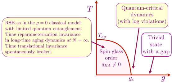
Figure 2: Phase diagram of the quantum Ising model in (4).

There is a phase with spin glass order at small $g$ and $T$, whose structure is similar to that of the classical model in Fig. 1. A theory of a quantum model necessarily involves dynamics, and so now we can define the spin glass order parameter by the autocorrelation function on a single site; at $T=0$ this is conveniently expressed in terms of the imaginary time ($\tau$) correlation

$$q_{EA}=\lim_{\tau\rightarrow\infty}\overline{\langle Z_{i}(\tau)Z_{i}(0)\rangle}\,.$$ (5)

We can move out of the spin glass phase either by raising temperature or by increasing $g$. In the latter case, we obtain a gapped paramagnetic ground state, smoothly connected to the trivial product state with all spins oriented in the $x$ direction. Near the quantum critical point at $g=g_{c}$, there is an interesting regime of quantum critical spin dynamics with a characteristic time of order $\hbar/(k_{B}T)$, with a logarithmic sensitivity to the magnitude of the exchange interactions $J$ [6, 7].

The real time quantum dynamics within the spin glass phase have mainly been studied for a spherical $p$-rotor quantum model [25, 26]. This model has many similarities to the Ising model, but has only one-step replica symmetry breaking, along with associated features in its dynamics. An important feature of the long-time glassy dynamics is the emergence of time reparameterization invariance at long times: the $N=\infty$ equations of motion for the spin autocorrelator $\mathcal{C}(t_{1},t_{2})$ are invariant under the transformation [20, 21, 22, 23, 24]

$$\mathcal{C}(t_{1},t_{2})\rightarrow\left[f^{\prime}(t_{1})f^{\prime}(t_{2})\right]^{\Delta}\mathcal{C}(f(t_{1}),C(f(t_{2}))$$ (6)

where $f(t)$ is a monotonic time reparameterization, and $\Delta$ is an exponent. However, despite this invariance, the solution to the full equations exhibits aging dynamics [23, 24, 25, 26, 27] in which time translational invariance is spontaneously broken. All these features are just as those for the classical model, and there are also connections between the aging dynamics and the structure of the replica symmetry breaking in the equilibrium solution.

4 Quantum Heisenberg model

Next, we consider quantum models without a trivial paramagnetic ground state because of LSM anomalies. For this, we need a spin model in which the on-site states remain doubly degenerate in the absence of couplings between the sites. We consider the ‘Heisenberg’ model with a global SU(2) spin rotation symmetry [61]

$$H_{3} =\frac{1}{2\sqrt{N}}\sum_{i,j=1}^{N}J_{ij}\left(X_{i}X_{j}+Y_{i}Y_{j}+Z_{i}Z_{j}\right)\,,$$ (7)

where $X_{i}$, $Y_{i}$, $Z_{i}$ are the 3 Pauli operators on each site. Such a model is connected to recent studies with ultracold atoms [62, 63, 64]. It is also useful to generalize this model to SU($M$) symmetry, and consider the phase diagram for general $M$ [30].

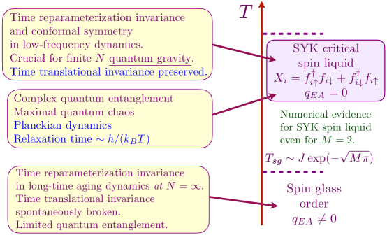
Figure 3: Phase diagram of the quantum Heisenberg model in (7), generalized to SU($M$) symmetry.

Fig. 3 sketches the basic features of the phase diagram of the SU($M$) spin models, as deduced from various studies [65, 30, 33, 66, 67, 26, 68, 69, 70, 71, 72, 73]. The low $T$ spin glass state is similar to that of the quantum Ising models, but a recent study has noted some interesting differences [73].

The remarkable new feature of Fig. 3 is the ‘SYK spin liquid’ regime which emerges in the intermediate temperature range $Je^{-\sqrt{\pi M}}<T<J$; there is evidence in Ref. [70] that such a regime is identifiable even for $M=2$. This regime is best understood as one in which there is complex quantum entanglement leading to fractionalization of the spins. Formally, we can rewrite $H_{3}$ exactly as a model of interacting fermions $f_{i\alpha}$, $\alpha=\uparrow,\downarrow$ by using the decomposition and constraints

$$(X_{i},Y_{i},Z_{i})=\frac{1}{2}f_{i\alpha}^{\dagger}{\bm\sigma}_{\alpha\beta}f_{i\beta}^{\phantom{\dagger}}\quad,\quad f_{i\alpha}^{\dagger}f_{i\alpha}^{\phantom{\dagger}}=1~{}\forall i\,,$$ (8)

where ${\bm\sigma}$ are the Pauli matrices. The SYK spin liquid appears when the $f_{i\alpha}$ fermions form the gapless critical state without quasiparticle excitations to be discussed in Section 6. The properties of this state are summarized in Fig. 3, and will be discussed further in Section 6. There is an emergent time reparameterization symmetry here, but it differs from that in the spin glass phase in important respects: (i) time translational symmetry is preserved, (ii) the large $N$ saddle-point has conformal symmetry. Both these features are crucial in the connection to quantum gravity discussed in Section 7.

An interesting recent proposal is that the SYK spin liquid state is present down to zero temperature in certain models even with SU(2) spins [74, 75, 76]. The important requirement is that the random two-spin interaction in (7) be replaced by 4 or higher spin interactions.

5 Free fermions

Before moving to the SYK model, it is useful to recall a few properties of a simple problem of free fermions with random hopping. We consider fermions $c_{i}$ with hopping amplitudes $t_{ij}$ which are independent random numbers, with Hamiltonian

$$H_{4}= \frac{1}{\sqrt{N}}\sum_{i,j=1}^{N}t_{ij}c_{i}^{\dagger}c_{j}-\mu\sum_{i}c_{i}^{\dagger}c_{i}$$ (9)

$$\overline{t_{ij}}=0,\quad \overline{|t_{ij}|^{2}}=t^{2},\quad\mbox{different $t_{ij}$ uncorrelated.}$$

This model is easily solved by determining the eigenvalues $\varepsilon_{\alpha}$ ($\alpha=1\ldots N$) of the random matrix $t_{ij}-\mu\delta_{ij}$. The distribution of these eigenvalues obeys Wigner-Dyson statistics: they are roughly equally spaced with a spacing of order $1/N$, and realize a semi-circular density of states, as shown in Fig. 4.

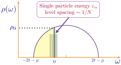
Figure 4: Single particle density of states of $H_{4}$.

Here $\rho(\omega)$ is the single particle density of states

$$\rho(\omega)=\frac{1}{N}\sum_{\alpha}\delta(\omega-\varepsilon_{\alpha})\,.$$ (10)

The many-particle ground state of $H_{4}$ is obtained by occupying all states with $\varepsilon_{\alpha}<0$. The familiar Sommerfeld theory yields the linear-$T$ dependence of the entropy at low $T$:

$$S(T\rightarrow 0)=N\gamma T\quad,\quad\gamma=\frac{\pi^{2}}{3}\rho_{0}\,,$$ (11)

where $\rho_{0}=\rho(0)$.

It is useful to map these results to a somewhat unfamiliar many-body perspective, as that will be useful in the comparison with the SYK model. In the grand-canonical ensemble, there are $2^{N}$ eigenstates $E_{0}+E_{a}$, $a=1\ldots 2^{N}$ given by

$$E_{0}+E_{a}=\sum_{\alpha}n_{\alpha}\varepsilon_{\alpha}$$ (12)

with $n_{\alpha}=0,1$, the occupation of the state $\alpha$. Here $E_{0}$ is the many-body ground state energy, chosen so that the smallest $E_{a}=0$. We now study the behavior of the many-boday density of states

$$D(E)=\sum_{a=1}^{2^{N}}\delta(E-E_{a})$$ (13)

This has not been computed analytically for all $E$ and we show numerical results for small $N$ in Fig. 5.

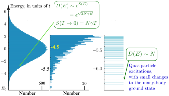
Figure 5: The many-body density of states of $H_{4}$. Adapted from numerics by G. Tarnopolsky and Ref. [65].

In the regime where $E$ is extensive (of order $N$), we can compute $D(E)$ by Boltzmann’s relation

$$D(E)\sim\exp(S(E))$$ (14)

where $S(E)$ is the entropy in the micro-canonical ensemble. This entropy can be obtained for $E\ll Nt$ (but of order $N$) from the grand-canonical result for $T\ll t$ in (11)

$$S(E)=\sqrt{2N\gamma E}\quad,\quad D(E)\sim\exp(\sqrt{2N\gamma E})\,.$$ (15)

So

$$\ln D(E)\sim N\quad,\quad E\sim N\,,$$ (16)

as expected in the thermodynamic limit.

Let us also consider the case when $E$ approaches zero, and is of order $1/N$. Then the many-body eigenstates are obtained by adding or removing a small number of particles near the Fermi level. As the single-particle level spacing is $\sim 1/N$ (see Fig. 4), we estimate

$$D(E)\sim N\quad,\quad E\sim 1/N\,.$$ (17)

6 SYK model

We now allow the fermions in the $\varepsilon_{\alpha}$ eigenstates of Section 5 to interact with each other. Given the random nature of these single-particle eigenstates, the matrix elements for interaction-induced transitions between these states will also be random. The complex SYK model [77, 78] is obtained by keeping only the random interactions in the Hamiltonian acting on the $2^{N}$ many-body states of Section 5:

$$H_{5}=\frac{1}{(2N)^{3/2}}\sum_{\alpha,\beta,\gamma,\delta=1}^{N}U_{\alpha\beta;\gamma\delta}\,c_{\alpha}^{\dagger}c_{\beta}^{\dagger}c_{\gamma}^{\vphantom{\dagger}}c_{\delta}^{\vphantom{\dagger}}-\mu\sum_{\alpha}c_{\alpha}^{\dagger}c_{\alpha}^{\vphantom{\dagger}}$$ (18)

$$\overline{U_{\alpha\beta;\gamma\delta}} =0,\quad\overline{|U_{\alpha\beta;\gamma\delta}|^{2}}=U^{2},\quad\mbox{different $U_{\alpha\beta;\gamma\delta}$ uncorrelated.}$$

It is also useful to define the charge density $\mathcal{Q}$

$$\mathcal{Q}=\frac{1}{N}\sum_{\alpha}c_{\alpha}^{\dagger}c_{\alpha}^{\vphantom{\dagger}}\,;\quad[{H}_{5},\mathcal{Q}]=0\,;\quad 0\leq\mathcal{Q}\leq 1\,.$$ (19)

There are now several experimental proposals or realizations of systems with SYK-like Hamiltonians [79, 80, 81, 82, 83, 84, 85, 86, 87, 88, 89, 90]

Numerical results for the spectrum of $H_{5}$ appear in Fig. 6.

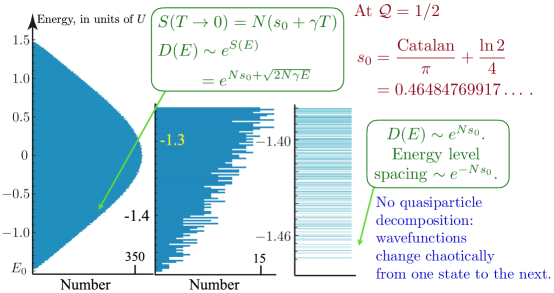
Figure 6: The many-body density of states of $H_{5}$. Adapted from numerics by G. Tarnopolsky and Ref. [65]. Compare to Fig 5, where $D(E)\sim N$ at low energy.

The important difference from the free fermion results in Fig. 5 is the exponentially larger density of states at low energies, as is discussed further below.

There is no glassy behavior in the ground state of the SYK model [91], and so we can proceed by examining only the replica diagonal sector. The averaged partition function of $H_{5}$ can be written as path integral over the bilocal fermion field $G(\tau_{1},\tau_{2})\sim({1}/{N})\sum_{\alpha}c_{\alpha}(\tau_{1})c_{\alpha}^{\dagger}(\tau_{2})$ [67, 32, 92, 77]

$$\overline{\mathcal{Z}}_{5}=\int\mathcal{D}G(\tau_{1},\tau_{2})\exp\left(-NS_{\rm eff}[G]\right)$$ (20)

The large $N$ saddle point equation $\delta S_{\rm eff}/\delta G=0$ yield a time-translational invariant solution for the fermion Green’s function $G_{s}(\tau_{1}-\tau_{2})=\left\langle G(\tau_{1},\tau_{2})\right\rangle$ [30]:

$$G_{s}(i\omega)=\frac{1}{i\omega+\mu-\Sigma_{s}(i\omega)}\quad ,\quad\Sigma_{s}(\tau)=-U^{2}G_{s}^{2}(\tau)G_{s}(-\tau)\,.$$ (21)

The solution of (21) yields the basic properties of the SYK critical state.

A key feature is the emergence of a time reparameterization symmetry at low frequencies and temperatures much smaller than $U$, where the $i\omega+\mu$ term in (21) can be neglected. Then the action $S_{\rm eff}[G]$ becomes invariant invariant under time reparametrization $f(\sigma)$ [31, 32]:

$$\tau =f(\sigma)$$

$$G(\tau_{1},\tau_{2}) =\left[f^{\prime}(\sigma_{1})f^{\prime}(\sigma_{2})\right]^{-1/4}\widetilde{G}(\sigma_{1},\sigma_{2})$$ (22)

Note the similarity of (22) to the classical time reparameterization in (6). Another key feature of the SYK critical state is that the saddle-point Green’s function has an invariance under SL(2, $R$) conformal transformations [33]:

$$G_{s}(\tau_{1}-\tau_{2})=\widetilde{G}_{s}(\sigma_{1}-\sigma_{2})~{}\text{for}~{}\tau=\frac{a\sigma+b}{c\sigma+d}\,,~{}ad-bc=1\,.$$ (23)

There is no analog of (23) for the spin glass state reparameterization in (6). The symmetry (23) will be crucial for the black hole mapping, as we will see in Section 7. The path integral in (20) also has an emergent U(1) gauge symmetry, linked to the presence of the conserved charge $\mathcal{Q}$ [77, 93, 78].

The time reparameterization and gauge symmetry are hints that the low energy effective theory of the SYK model is a theory of gravity and electromagnetism. Indeed, the theory turns out to be just Einstein-Maxwell theory in the background of a charged black hole, as will be discussed further in Section 7. Furthermore, the path integral in (20) can be exactly evaluated for this effective theory [31, 32, 94, 95, 96, 78], leading to the following finite $N$ results for the low energy many-body density of states in the ensemble with a fixed $\mathcal{Q}$ [78]:

$$D(E,\mathcal{Q})\sim\frac{1}{N}\exp(Ns_{0})\sinh\left(\sqrt{2N\gamma E}\right)\,,\quad E\ll NU\,.$$ (24)

The number $s_{0}$ is a universal function of $\mathcal{Q}$, computed in Ref. [67]. For extensive $E$, the $E$ dependence of (24) is the same as (15) for the free fermion model, but with an exponentially large $E$-independent prefactor.

$$D(E,\mathcal{Q})\sim\exp(Ns_{0})\exp(\sqrt{2N\gamma E})\quad,\quad E\sim N\,.$$ (25)

However, for small $E$ there is a dramatic difference from the free fermion model, as indicated in Figs. 5 and 6, with

$$D(E,\mathcal{Q})\sim\sqrt{\frac{E}{N}}\exp(Ns_{0})\quad,\quad E\ll 1/N\,,$$ (26)

in contrast to (17).

The partition function of the SYK model is related to (24) by

$$\overline{\mathcal{Z}}_{5}(T,\mathcal{Q})=\int_{0}^{\infty}dED(E,\mathcal{Q})e^{-E/T}\,.$$ (27)

For the canonical entropy of the SYK model at low $T$, (27) yields [32, 92, 78]

$$S(T,\mathcal{Q})=N(s_{0}+\gamma T)-\frac{3}{2}\ln\left(\frac{U}{T}\right)-\frac{1}{2}\ln N\,.$$ (28)

Comparing to the free fermion result in (11), we notice an extensive entropy $Ns_{0}$ in the low $T$ limit [67], and this will map to the $T=0$ Bekenstein-Hawking entropy of charged black holes in Section 7. Note that the ground state is not degenerate, and this extensive entropy does not imply an exponentially large ground state degeneracy: the latter requires $T\rightarrow 0$ before $N\rightarrow\infty$, and here we are taking the opposite order of limits. The sub-extensive term in (28) has a singular $-(3/2)\ln(1/T)$ dependence on temperature, and this implies that the expansion in (28) breaks down at a temperature exponentially small in $N$. Given the exponentially small level spacing near the ground state (see Fig. 6), this is reasonable because we have to account for the discreteness of the energy levels at such low $T$.

7 Quantum black holes

See Ref. [97] for a more detailed review of the topics discussed in this section.

A key fact linking charged black holes to the SYK model is illustrated in Fig. 7: the solution of the Einstein-Maxwell equations for a black hole with a net charge $\mathcal{Q}$ in spatial dimensions $d\geq 3$ yields a near-horizon metric with a AdS₂ factor [98, 99, 100]. And the isometry of AdS₂ is SL(2, $R$) identical to the symmetry of the SYK saddle point in (23). The AdS₂ metric in Euclidean time is

$$ds^{2}=\frac{d\tau^{2}+d\zeta^{2}}{\zeta^{2}}\,,$$ (29)

and this is invariant under the co-ordinate change

$$\tau^{\prime}+i\zeta^{\prime}=\frac{a(\tau+i\zeta)+b}{c(\tau+i\zeta)+d}\,,\quad ad-bc=1\,.$$ (30)

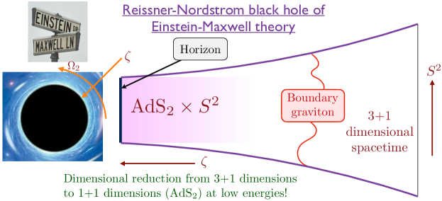
Figure 7: Near-horizon AdS₂ geometry of charged black holes.

Gibbons and Hawking [101] proposed to determine the quantum thermodynamics of a black hole by computing the path integral of Einstein-Maxwell theory in imaginary time outside the black hole horizon. The black hole metric in imaginary time has a cigar geometry which closes off at the horizon, and so this allowed them to sidestep the lack of knowledge of the black hole interior. They evaluated the partition function of a black hole with charge $\mathcal{Q}$ in an asymptotically 3+1 dimensional Minkowski spacetime

$$\mathcal{Z}_{6}(\mathcal{Q},T)=\int\mathcal{D}g_{\mu\nu}\mathcal{D}A_{\mu}\exp\left(-\frac{1}{\hbar}~{}I^{(3+1)}_{\mathrm{Einstein~{}gravity}+\mathrm{Maxwell~{}EM}}[g_{\mu\nu},A_{\mu}]\right)\,,$$ (31)

where $g_{\mu\nu}$ is the spacetime metric, and $A_{\mu}$ is the electromagnetic vector potential. In the semiclassical saddle-point approximation, they obtained

$$\mathcal{Z}_{6}(\mathcal{Q},T)=\exp\Bigl{(}-F_{BH}/T\Bigr{)}\times\Biggl{(}\quad....????...\quad\Biggr{)}\,,$$ (32)

where $F_{BH}$ is the free energy, and $S_{BH}=-\partial F_{BH}/\partial T$ is the Bekenstein-Hawking entropy. In the low $T$ limit at fixed $\mathcal{Q}$, this is

$$S_{BH}(T\rightarrow 0,\mathcal{Q}) =\frac{{\mathcal{A}}(T)c^{3}}{4\hbar G}=\frac{{\mathcal{A}}_{0}c^{3}}{4\hbar G}\left(1+\frac{2\sqrt{\pi{\mathcal{A}}_{0}}\,T}{\hbar c}+\ldots\right)\,,$$ (33)

where $G$ is Newton’s constant, $c$ is the velocity of light, $\hbar$ is Planck’s constant, and ${\mathcal{A}}(T)$ is the area of the charged black hole horizon with

$${\mathcal{A}}_{0}\equiv{\mathcal{A}}(T\rightarrow 0)=\frac{2G\mathcal{Q}^{2}}{c^{4}}\,.$$ (34)

Notice the similarity of the $T$ dependence of (33) to the extensive terms in (28), another key fact pointing to the connection to the SYK model [34].

We now exploit the technology developed for the SYK model to evaluate $\mathcal{Z}_{6}$ beyond the Gibbons-Hawking saddle-point approximation. Using the dimensional reduction in Fig. 7, it can be shown that [102, 36, 37, 38, 78]

$$\mathcal{Z}_{6}(\mathcal{Q},T)$$

$$\approx\exp\left(\frac{{\mathcal{A}}_{0}c^{3}}{4\hbar G}\right)\int\mathcal{D}g_{\mu\nu}\mathcal{D}A_{\mu}\exp\left(-\frac{1}{\hbar}~{}I^{(1+1)}_{\mathrm{JT~{}gravity~{}of~{}AdS}_{2}+\mathrm{boundary~{}graviton}}[g_{\mu\nu},A_{\mu}]\right)$$

$$=\exp\left(\frac{{\mathcal{A}}_{0}c^{3}}{4\hbar G}\right)\int\mathcal{D}f(\tau)\mathcal{D}\phi(\tau)$$

$$~{}~{}~{}~{}~{}\times\exp\left(-\frac{1}{\hbar}I^{0+1}_{{\rm SYK}}[\mbox{time reparameterizations $f(\tau)$, phase rotations $\phi(\tau)$}]\right)\,.$$ (35)

Here JT gravity is an effective 1+1 dimensional gravity theory obtained from the dimensional reduction, and this describes the dynamics of the boundary graviton in Fig. 7. Remarkably the JT gravity theory is exactly equivalent to the 0+1 dimensional theory $I^{0+1}_{\rm SYK}$ of time reparameterizations $f(\tau)$ and U(1) phase fluctuations $\phi(\tau)$ obtained from the low energy limit of the SYK action $S_{\rm eff}[G]$ in (20). The theory $I^{0+1}_{\rm SYK}$ contains a Schwarzian action for $f(\tau)$. The final result [35, 36, 38, 39, 37] for the black hole density of states is obtained by evaluating the path integral in (35), using (27), and fixing the overall prefactor [39] by the low-energy physics of the 4-dimensional spacetime

$$D(E,\mathcal{Q})\sim\left(\frac{{\mathcal{A}}_{0}c^{3}}{\hbar G}\right)^{-347/90}\exp\left(\frac{{\mathcal{A}}_{0}c^{3}}{4\hbar G}\right)\sinh\left(\left[\frac{\sqrt{\pi}{\mathcal{A}}_{0}^{3/2}c^{2}}{\hbar^{2}G}E\right]^{1/2}\right)\,,$$ (36)

where ${\mathcal{A}}_{0}$ is given by (34). Notice the striking similarity to (24) for the SYK model. The exponential and sinh factors are in one-to-one correspondence, and in both cases the remaining pre-factor relies upon physics beyond the low energy path integral in (35).

Collecting these results, we also determine the unknown corrections in (32) and (33), and obtain the low $T$ limit of the entropy at fixed $\mathcal{Q}$:

$$S(T,\mathcal{Q}) =\frac{{\mathcal{A}}_{0}c^{3}}{4\hbar G}\left(1+\frac{2\sqrt{\pi{\mathcal{A}}_{0}}\,T}{\hbar c}\right)-\frac{3}{2}\ln\left(\frac{\sqrt{\hbar c^{5}/G}}{T}\right)-\frac{559}{180}\ln\left(\frac{{\mathcal{A}}_{0}c^{3}}{\hbar G}\right)\,.$$ (37)

Again, note the close similarity to (28) for the SYK model, with the surface area of the black hole in Planck units ${\mathcal{A}}_{0}c^{3}/(\hbar G)$, and the number of fermionic qubits in the SYK model $N$, playing equivalent roles. Also, the Planck energy $\sqrt{\hbar c^{5}/G}$ maps to the root-mean-square strength of the SYK interactions $U$. The first 3 terms in (37) are universal in that they apply to any quantum theory of gravity whose low energy limit is non-supersymmetric Einstein-Maxwell theory; a similar universality applies to (28) for a wide class of SYK-type models. Only the co-efficient on the second logarithm in (37) depends upon more microscopic information [39, 35], as does the co-efficient of the second logarithm in (28) [78].

Finally, we note that the evaluation of black hole entropy in string theory [103] relied upon supersymmetry, where the entropy is realized by an exponentially large ground state degeneracy that is present both in supersymmetric SYK models [40] and black holes [104]. Here we have described the generic behavior without low energy supersymmetry, where there is no significant ground state degeneracy. The non-supersymmetric case does have a zero temperature entropy obtained in the limit $T\rightarrow 0$ after $N\rightarrow\infty$, linked to the exponentially small level spacing near the ground state shown in Fig. 6. The ground state degeneracy is associated with the opposite order of limits (as we noted below (28)), and it is exponentially large only with supersymmetry.

8 Universal theory of strange metals

Understanding the ubiquitous strange metal state of correlated electron materials has been a long-standing challenge in quantum condensed matter physics [65, 105]. There have been numerous attempts to make the SYK model (20) more realistic by giving it spatial structure by allowing the fermions to hop on a lattice. These attempts have given much insight, but left key issues open: they do give regimes of linear-in-$T$ resistivity, but the low $T$ behavior is inevitably that of a disordered Fermi liquid [65].

Rapid progress has been made recently starting from ‘Yukawa-SYK’ models which randomly couple the fermions to bosons [40, 41, 42, 43, 44, 45, 46, 47, 48, 49, 50]. The simplest such model has only dispersionless fermions $\psi_{i}$ and Einstein oscillators $\phi_{\ell}$ with the same frequency $\omega_{0}$, coupled to each other with a random Yukawa coupling $g_{ij\ell}$ [44, 45]:

$$H_{7}=-\mu\sum_{i}\psi_{i}^{\dagger}\psi_{i}+\sum_{\ell}\frac{1}{2}\left(\pi_{\ell}^{2}+\omega_{0}^{2}\phi_{\ell}^{2}\right)+\sum_{ij\ell}g_{ij\ell}\psi_{i}^{\dagger}\psi_{j}\phi_{\ell}$$ (38)

$$~{}~{}~{}~{}\overline{g_{ij\ell}}=0,\quad\overline{|g_{ij\ell}|^{2}}=g^{2},\quad\mbox{different $g_{ij\ell}$ uncorrelated.}$$

This model can be solved exactly in the large $N$ limit, and displays a SYK critical state with properties very similar to those of the SYK model in Section 6, including the emergent time reparameterization symmetry. The model $H_{7}$ also has a superconducting state, but we will not explore that here.

We now wish to make $H_{7}$ more realistic. As an example, consider the Hertz-Millis theory of quantum phase transition in a metal associated with a density wave order parameter $\phi_{a}$ ($a=1\ldots M$) [106] (similar considerations apply also Fermi-volume changing transitions involving fractionalized bosons [105]). The transition is between a phase with $\langle\phi\rangle\neq 0$ and a phase with $\langle\phi\rangle=0$. In the presence of spatial disorder, we can write the following general Lagrangian [54, 57]

$$\mathcal{L}_{8}= \psi_{{\bm k}}^{\dagger}\left(\frac{\partial}{\partial\tau}+\varepsilon({\bm k})\right)\psi_{\bm k}+[s+{\color[rgb]{0,0,1}\delta s({\bm r})}]\,[\phi({\bm r})]^{2}+e^{i{\bm G}\cdot{\bm r}}[g+{\color[rgb]{0,0,1}g^{\prime}({\bm r})}]\,\psi^{\dagger}({\bm r})\,\mathcal{M}\,\psi({\bm r})\,\phi({\bm r})$$

$$~{}~{}~{}~{}~{}~{}~{}~{}+K\,[\nabla_{\bm r}\phi({\bm r})]^{2}+u\,[\phi({\bm r})]^{4}+{\color[rgb]{0,0,1}v({\bm r})}\psi^{\dagger}({\bm r})\psi({\bm r})\,,$$ (39)

where the couplings with a fixed random dependence on space are shown in blue. In comparison to $H_{7}$, in $\mathcal{L}_{8}$ we have given the fermions a Fermi surface associated with the dispersion $\varepsilon({\bm k})$, and a spatial field theory for the scalar field $\phi$ in $d=2$ spatial dimensions. The coupling matrix $\mathcal{M}$ and the ordering wavevector ${\bm G}$ are fixed, and their form depends upon the particular symmetry being broken. The transition is tuned by varying the boson ‘mass’ $s$. Crucial to our considerations are the ${\bm r}$ dependent couplings which represent the spatial disorder; these obey the disorder averages

• Spatially random Yukawa coupling ${\color[rgb]{0,0,1}g^{\prime}({\bm r})}$ with ${\color[rgb]{0,0,1}\overline{g^{\prime}({\bm r})}=0}$,
  ${\color[rgb]{0,0,1}\overline{g^{\prime}({\bm r})g^{\prime}({\bm r^{\prime}})}=g^{\prime 2}\delta({\bm r}-{\bm r^{\prime}})}$.

• Spatially random mass ${\color[rgb]{0,0,1}\delta s({\bm r})}$ with ${\color[rgb]{0,0,1}\overline{\delta s({\bm r})}=0}$, ${\color[rgb]{0,0,1}\overline{\delta s({\bm r})\delta s({\bm r^{\prime}})}=\delta s^{2}\delta({\bm r}-{\bm r^{\prime}})}$.

• Spatially random potential ${\color[rgb]{0,0,1}v({\bm r})}$ with ${\color[rgb]{0,0,1}\overline{v({\bm r})}=0}$, ${\color[rgb]{0,0,1}\overline{v({\bm r})v({\bm r^{\prime}})}=v^{2}\delta({\bm r}-{\bm r^{\prime}})}$.

A standard analysis of $\mathcal{L}_{8}$ for weak disorder shows that the random mass disorder ${\color[rgb]{0,0,1}\delta s({\bm r})}$ is the strongest relevant perturbation at the quantum phase transition [107]. This is a consequence of the violation of the Harris criterion $\nu>2/d$ [108], and the value $\nu=1/2$ in $d=2$. Recent work has developed the following approach for dealing with this strongly relevant perturbation, combining SYK-like disorder-self-averaging [51, 52, 53, 54, 55, 56, 57] with methods based on the strong disorder renormalization group [109, 110, 111].

• We can account for the spatial dependence of ${\color[rgb]{0,0,1}\delta s({\bm r})}$ by expressing the $\phi$ quantum fluctuations in a new basis which diagonalizes the $\phi$ quadratic form [54]. As long as the $\phi$ eigenstates remain extended, we expect a diffusive form for the $\phi$ propagator [112]. But the transformation to this new basis induces disorder in the Yukawa coupling, and in particular, makes ${\color[rgb]{0,0,1}g^{\prime}({\bm r})}$ non-zero even in previously common theories without initial disorder in the Yukawa coupling. We further assume that in this regime of extended $\phi$ eigenstates we can treat the ${\color[rgb]{0,0,1}g^{\prime}({\bm r})}$ and ${\color[rgb]{0,0,1}v({\bm r})}$ disorder in a self-averaging manner, similar to that in the SYK model. Then we obtain self-consistent equations for the boson and fermion Green’s functions analogous to (21) for the SYK model; because of the spatial dimensionality $d=2$, these equations involve Green’s functions with momentum and position arguments. The SYK method can also be extended to compute transport properties [55]. The results from such computations agree with numerous observations on strange metals at intermediate temperatures, including the $T$-dependent resistivity, the optical conductivity [113], the specific heat, and the marginal Fermi liquid behavior of the electron spectral function [114].

• At very low $T$, we can expect the $\phi$ eigenmodes to localize, and then ${\color[rgb]{0,0,1}\delta s({\bm r})}$ cannot be treated in a self-averaging manner [57]. From an application of the strong disorder renormalization group to large ${\color[rgb]{0,0,1}|\delta s({\bm r})|}$, Hoyos et al. [110] proposed that the lowest energy bosonic eigenmodes have a structure very similar to that of the random quantum Ising model, specifically to the extension of the model $H_{2}$ in (4) to the ferromagnetic case with a non-zero $J_{ij}$ average in spatial dimension $d=2$ [109]. Numerical evidence for this strong disorder regime, and its consequences for strange metal transport were presented in Ref. [57].

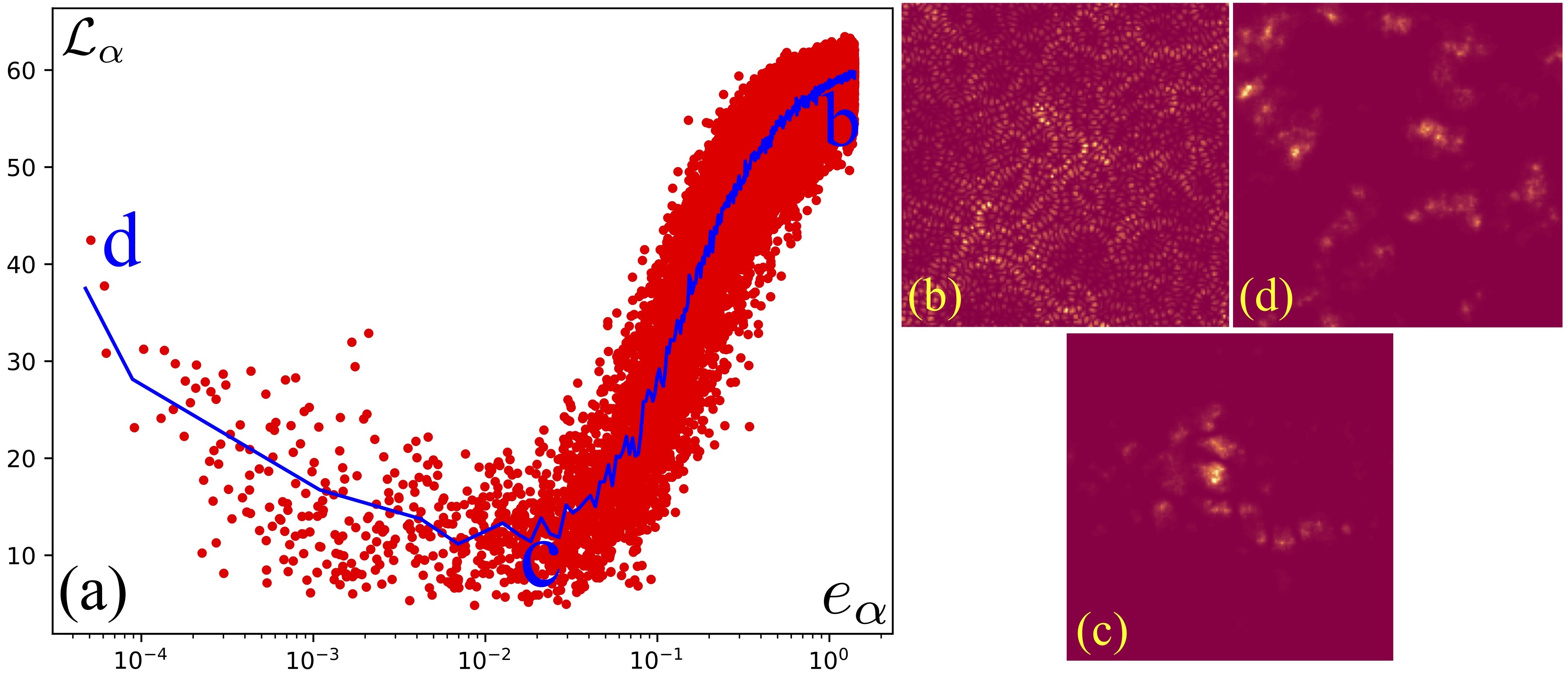
Figure 8: From Ref. [57]. (a) Localization length $\mathcal{L}_{\alpha}$ of overdamped bosonic eigenmodes of (39) as a function of their energy $e_{\alpha}$, computed in a large $M$ limit. (b,c,d) Pictures of the corresponding bosonic eignfunctions. The self-averaging SYK-like theory applies to (b), while the mapping to the random Ising model applies to (d).

Fig. 8 shows numerical results for the localization length of the bosonic eigenmodes from Ref. [57] which justify the above analyses. The non-monotonic behavior of as a function of energy in Fig. 8a clearly demonstrates the two regimes described above. At higher energies, we have extended states for which the self-averaging SYK methods work well. At very low energy, we obtain strong disorder dominated overdamped bosonic modes, whose localization length increases logarithmically slowly with decreasing energy—this is just as expected from the random quantum Ising model [109].

The results of the analyses described above capture the main features of the global phase diagram of strange metals [57], including the ‘foot’ feature which extends strange metal behavior at low $T$ beyond the usual quantum critical region [115].

References

- [1] T. Yamamoto and H. Ishii, A perturbation expansion for the Sherrington-Kirkpatrick model with a transverse field, J. Phys. C: Solid State Phys. 20 (1987) 6053.
- [2] T.K. Kopeć, K.D. Usadel and G. Büttner, Instabilities in the quantum Sherrington-Kirkpatrick Ising spin glass in transverse and longitudinal fields, Phys. Rev. B 39 (1989) 12418.
- [3] P. Ray, B.K. Chakrabarti and A. Chakrabarti, Sherrington-Kirkpatrick model in a transverse field: Absence of replica symmetry breaking due to quantum fluctuations, Phys. Rev. B 39 (1989) 11828.
- [4] G. Büttner and K.D. Usadel, Stability analysis of an Ising spin glass with transverse field, Phys. Rev. B 41 (1990) 428.
- [5] J. Miller and D.A. Huse, Zero-temperature critical behavior of the infinite-range quantum Ising spin glass, Phys. Rev. Lett. 70 (1993) 3147.
- [6] J. Ye, S. Sachdev and N. Read, Solvable spin glass of quantum rotors, Phys. Rev. Lett. 70 (1993) 4011 [cond-mat/9212027].
- [7] N. Read, S. Sachdev and J. Ye, Landau theory of quantum spin glasses of rotors and Ising spins, Phys. Rev. B 52 (1995) 384 [cond-mat/9412032].
- [8] M.J. Rozenberg and D.R. Grempel, Dynamics of the Infinite-Range Ising Spin-Glass Model in a Transverse Field, Phys. Rev. Lett. 81 (1998) 2550.
- [9] M.P. Kennett, C. Chamon and J. Ye, Aging dynamics of quantum spin glasses of rotors, Phys. Rev. B 64 (2001) 224408 [cond-mat/0103428].
- [10] L. Arrachea and M.J. Rozenberg, Dynamical Response of Quantum Spin-Glass Models at , Phys. Rev. Lett. 86 (2001) 5172.
- [11] A. Andreanov and M. Müller, Long-Range Quantum Ising Spin Glasses at : Gapless Collective Excitations and Universality, Phys. Rev. Lett. 109 (2012) 177201.
- [12] S. Mukherjee, A. Rajak and B.K. Chakrabarti, Classical-to-quantum crossover in the critical behavior of the transverse-field Sherrington-Kirkpatrick spin glass model, Phys. Rev. E 92 (2015) 042107 [1412.2973].
- [13] S. Mukherjee, A. Rajak and B.K. Chakrabarti, Possible ergodic-nonergodic regions in the quantum Sherrington-Kirkpatrick spin glass model and quantum annealing, Phys. Rev. E 97 (2018) 022146 [1706.01446].
- [14] A.P. Young, Stability of the quantum Sherrington-Kirkpatrick spin glass model, Phys. Rev. E 96 (2017) 032112 [1707.07107].
- [15] A. Kiss, G. Zaránd and I. Lovas, Exact Solution for the Transverse Field Sherrington-Kirkpatrick Spin Glass Model with Continuous-Time Quantum Monte Carlo Method, 2306.07337.
- [16] M. Tikhanovskaya, S. Sachdev and R. Samajdar, Equilibrium dynamics of infinite-range quantum spin glasses in a field, arXiv e-prints (2023) arXiv:2309.03255 [2309.03255].
- [17] D. Sherrington and S. Kirkpatrick, Solvable model of a spin-glass, Phys. Rev. Lett. 35 (1975) 1792.
- [18] G. Parisi, Infinite Number of Order Parameters for Spin-Glasses, Phys. Rev. Lett. 43 (1979) 1754.
- [19] K. Fischer and J. Hertz, Spin Glasses, Cambridge University Press, Cambridge (1993), 10.1017/CBO9780511628771.
- [20] H. Sompolinsky and A. Zippelius, Dynamic Theory of the Spin-Glass Phase, Phys. Rev. Lett. 47 (1981) 359.
- [21] H. Sompolinsky, Time-Dependent Order Parameters in Spin-Glasses, Phys. Rev. Lett. 47 (1981) 935.
- [22] H. Sompolinsky and A. Zippelius, Relaxational dynamics of the Edwards-Anderson model and the mean-field theory of spin-glasses, Phys. Rev. B 25 (1982) 6860.
- [23] L.F. Cugliandolo and J. Kurchan, On the out-of-equilibrium relaxation of the Sherrington-Kirkpatrick model, J. Phys. A: Math. Gen. 27 (1994) 5749 [cond-mat/9311016].
- [24] L.F. Cugliandolo and J. Kurchan, Weak ergodicity breaking in mean-field spin-glass models, Philosophical Magazine, Part B 71 (1995) 501 [cond-mat/9403040].
- [25] L.F. Cugliandolo and G. Lozano, Real-time nonequilibrium dynamics of quantum glassy systems, Phys. Rev. B 59 (1999) 915 [cond-mat/9807138].
- [26] G. Biroli and O. Parcollet, Out-of-equilibrium dynamics of a quantum Heisenberg spin glass, Phys. Rev. B 65 (2002) 094414 [cond-mat/0105001].
- [27] S.J. Thomson, P. Urbani and M. Schiró, Quantum Quenches in Isolated Quantum Glasses out of Equilibrium, Phys. Rev. Lett. 125 (2020) 120602 [1904.03147].
- [28] N. Read and S. Sachdev, Valence-bond and spin-Peierls ground states of low-dimensional quantum antiferromagnets, Phys. Rev. Lett. 62 (1989) 1694.
- [29] N. Read and S. Sachdev, Large- expansion for frustrated quantum antiferromagnets, Phys. Rev. Lett. 66 (1991) 1773.
- [30] S. Sachdev and J. Ye, Gapless spin-fluid ground state in a random quantum Heisenberg magnet, Phys. Rev. Lett. 70 (1993) 3339 [cond-mat/9212030].
- [31] A.Y. Kitaev, Talks at KITP, University of California, Santa Barbara, Entanglement in Strongly-Correlated Quantum Matter (2015) .
- [32] J. Maldacena and D. Stanford, Remarks on the Sachdev-Ye-Kitaev model, Phys. Rev. D 94 (2016) 106002 [1604.07818].
- [33] O. Parcollet and A. Georges, Non-Fermi-liquid regime of a doped Mott insulator, Phys. Rev. B 59 (1999) 5341 [cond-mat/9806119].
- [34] S. Sachdev, Holographic metals and the fractionalized Fermi liquid, Phys. Rev. Lett. 105 (2010) 151602 [1006.3794].
- [35] S. Banerjee, R.K. Gupta and A. Sen, Logarithmic Corrections to Extremal Black Hole Entropy from Quantum Entropy Function, JHEP 03 (2011) 147 [1005.3044].
- [36] U. Moitra, S.P. Trivedi and V. Vishal, Extremal and near-extremal black holes and near-CFT1, Journal of High Energy Physics 07 (2019) 055 [1808.08239].
- [37] S. Sachdev, Universal low temperature theory of charged black holes with AdS2 horizons, J. Math. Phys. 60 (2019) 052303 [1902.04078].
- [38] L.V. Iliesiu and G.J. Turiaci, The statistical mechanics of near-extremal black holes, JHEP 05 (2021) 145 [2003.02860].
- [39] L.V. Iliesiu, S. Murthy and G.J. Turiaci, Revisiting the Logarithmic Corrections to the Black Hole Entropy, arXiv e-prints (2022) [2209.13608].
- [40] W. Fu, D. Gaiotto, J. Maldacena and S. Sachdev, Supersymmetric Sachdev-Ye-Kitaev models, Phys. Rev. D 95 (2017) 026009 [1610.08917].
- [41] J. Murugan, D. Stanford and E. Witten, More on Supersymmetric and 2d Analogs of the SYK Model, JHEP 08 (2017) 146 [1706.05362].
- [42] A.A. Patel and S. Sachdev, Critical strange metal from fluctuating gauge fields in a solvable random model, Phys. Rev. B 98 (2018) 125134 [1807.04754].
- [43] E. Marcus and S. Vandoren, A new class of SYK-like models with maximal chaos, JHEP 01 (2019) 166 [1808.01190].
- [44] Y. Wang, Solvable Strong-coupling Quantum Dot Model with a Non-Fermi-liquid Pairing Transition, Phys. Rev. Lett. 124 (2020) 017002 [1904.07240].
- [45] I. Esterlis and J. Schmalian, Cooper pairing of incoherent electrons: an electron-phonon version of the Sachdev-Ye-Kitaev model, Phys. Rev. B 100 (2019) 115132 [1906.04747].
- [46] Y. Wang and A.V. Chubukov, Quantum Phase Transition in the Yukawa-SYK Model, Phys. Rev. Res. 2 (2020) 033084 [2005.07205].
- [47] W. Wang, A. Davis, G. Pan, Y. Wang and Z.Y. Meng, Phase diagram of the spin-1/2 Yukawa-Sachdev-Ye-Kitaev model: Non-Fermi liquid, insulator, and superconductor, Phys. Rev. B 103 (2021) 195108 [2102.10755].
- [48] H. Guo, D. Valentinis, J. Schmalian, S. Sachdev and A.A. Patel, Cyclotron resonance and quantum oscillations of critical Fermi surfaces, Phys. Rev. B 109 (2024) 075162 [2302.13134].
- [49] D. Valentinis, G.A. Inkof and J. Schmalian, BCS to incoherent superconductivity crossovers in the Yukawa-SYK model on a lattice, arXiv e-prints (2023) [2302.13138].
- [50] H. Hosseinabadi, S.P. Kelly, J. Schmalian and J. Marino, Thermalization of non-Fermi-liquid electron-phonon systems: Hydrodynamic relaxation of the Yukawa-Sachdev-Ye-Kitaev model, Phys. Rev. B 108 (2023) 104319 [2306.03898].
- [51] E.E. Aldape, T. Cookmeyer, A.A. Patel and E. Altman, Solvable theory of a strange metal at the breakdown of a heavy Fermi liquid, Phys. Rev. B 105 (2022) 235111 [2012.00763].
- [52] I. Esterlis, H. Guo, A.A. Patel and S. Sachdev, Large theory of critical Fermi surfaces, Phys. Rev. B 103 (2021) 235129 [2103.08615].
- [53] M. Tikhanovskaya, S. Sachdev and A.A. Patel, Maximal Quantum Chaos of the Critical Fermi Surface, Phys. Rev. Lett. 129 (2022) 060601 [2202.01845].
- [54] A.A. Patel, H. Guo, I. Esterlis and S. Sachdev, Universal theory of strange metals from spatially random interactions, Science 381 (2022) 790 [2203.04990].
- [55] H. Guo, A.A. Patel, I. Esterlis and S. Sachdev, Large- theory of critical Fermi surfaces. II. Conductivity, Phys. Rev. B 106 (2022) 115151 [2207.08841].
- [56] H. Guo, D. Valentinis, J. Schmalian, S. Sachdev and A.A. Patel, Cyclotron resonance and quantum oscillations of critical Fermi surfaces, arXiv e-prints (2023) arXiv:2308.01956 [2308.01956].
- [57] A.A. Patel, P. Lunts and S. Sachdev, Localization of overdamped bosonic modes and transport in strange metals, arXiv e-prints (2023) arXiv:2312.06751 [2312.06751].
- [58] S. Ebadi, A. Keesling, M. Cain, T.T. Wang, H. Levine, D. Bluvstein et al., Quantum optimization of maximum independent set using Rydberg atom arrays, Science 376 (2022) 1209 [2202.09372].
- [59] A.D. King, J. Raymond, T. Lanting, R. Harris, A. Zucca, F. Altomare et al., Quantum critical dynamics in a 5,000-qubit programmable spin glass, Nature 617 (2023) 61 [2207.13800].
- [60] F.B. Maciejewski, S. Hadfield, B. Hall, M. Hodson, M. Dupont, B. Evert et al., Design and execution of quantum circuits using tens of superconducting qubits and thousands of gates for dense Ising optimization problems, arXiv e-prints (2023) arXiv:2308.12423 [2308.12423].
- [61] A.J. Bray and M.A. Moore, Replica theory of quantum spin glasses, Journal of Physics C: Solid State Physics 13 (1980) L655.
- [62] E.S. Cooper, P. Kunkel, A. Periwal and M. Schleier-Smith, Engineering Graph States of Atomic Ensembles by Photon-Mediated Entanglement, arXiv e-prints (2022) arXiv:2212.11961 [2212.11961].
- [63] F. Finger, R. Rosa-Medina, N. Reiter, P. Christodoulou, T. Donner and T. Esslinger, Spin- and momentum-correlated atom pairs mediated by photon exchange and seeded by vacuum fluctuations, arXiv e-prints (2023) arXiv:2303.11326 [2303.11326].
- [64] R.M. Kroeze, B.P. Marsh, D. Atri Schuller, H.S. Hunt, S. Gopalakrishnan, J. Keeling et al., Replica symmetry breaking in a quantum-optical vector spin glass, arXiv e-prints (2023) arXiv:2311.04216 [2311.04216].
- [65] D. Chowdhury, A. Georges, O. Parcollet and S. Sachdev, Sachdev-Ye-Kitaev models and beyond: Window into non-Fermi liquids, Rev. Mod. Phys. 94 (2022) 035004 [2109.05037].
- [66] A. Georges, O. Parcollet and S. Sachdev, Mean Field Theory of a Quantum Heisenberg Spin Glass, Phys. Rev. Lett. 85 (2000) 840 [cond-mat/9909239].
- [67] A. Georges, O. Parcollet and S. Sachdev, Quantum fluctuations of a nearly critical Heisenberg spin glass, Phys. Rev. B 63 (2001) 134406 [cond-mat/0009388].
- [68] L. Arrachea and M.J. Rozenberg, Infinite-range quantum random Heisenberg magnet, Phys. Rev. B 65 (2002) 224430 [cond-mat/0203537].
- [69] A. Camjayi and M.J. Rozenberg, Quantum and Thermal Fluctuations in the SU() Heisenberg Spin-Glass Model near the Quantum Critical Point, Phys. Rev. Lett. 90 (2003) 217202 [cond-mat/0210407].
- [70] H. Shackleton, A. Wietek, A. Georges and S. Sachdev, Quantum Phase Transition at Nonzero Doping in a Random - Model, Phys. Rev. Lett. 126 (2021) 136602 [2012.06589].
- [71] P.T. Dumitrescu, N. Wentzell, A. Georges and O. Parcollet, Planckian metal at a doping-induced quantum critical point, Phys. Rev. B 105 (2022) L180404 [2103.08607].
- [72] M. Christos, F.M. Haehl and S. Sachdev, Spin liquid to spin glass crossover in the random quantum Heisenberg magnet, Phys. Rev. B 105 (2022) 085120 [2110.00007].
- [73] N. Kavokine, M. Müller, A. Georges and O. Parcollet, Exact numerical solution of the classical and quantum Heisenberg spin glass, arXiv e-prints (2023) arXiv:2312.14598 [2312.14598].
- [74] M. Hanada, A. Jevicki, X. Liu, E. Rinaldi and M. Tezuka, A model of randomly-coupled Pauli spins, arXiv e-prints (2023) arXiv:2309.15349 [2309.15349].
- [75] B. Swingle and M. Winer, A Bosonic Model of Quantum Holography, arXiv e-prints (2023) arXiv:2311.01516 [2311.01516].
- [76] E.R. Anschuetz, D. Gamarnik and B.T. Kiani, Product states optimize quantum -spin models for large , arXiv e-prints (2023) arXiv:2309.11709 [2309.11709].
- [77] S. Sachdev, Bekenstein-Hawking Entropy and Strange Metals, Phys. Rev. X 5 (2015) 041025 [1506.05111].
- [78] Y. Gu, A. Kitaev, S. Sachdev and G. Tarnopolsky, Notes on the complex Sachdev-Ye-Kitaev model, Journal of High Energy Physics 02 (2020) 157 [1910.14099].
- [79] A. Chew, A. Essin and J. Alicea, Approximating the Sachdev-Ye-Kitaev model with Majorana wires, Phys. Rev. B 96 (2017) 121119 [1703.06890].
- [80] D.I. Pikulin and M. Franz, Black Hole on a Chip: Proposal for a Physical Realization of the Sachdev-Ye-Kitaev model in a Solid-State System, Physical Review X 7 (2017) 031006 [1702.04426].
- [81] L. García-Álvarez, I.L. Egusquiza, L. Lamata, A. del Campo, J. Sonner and E. Solano, Digital Quantum Simulation of Minimal AdS/CFT, Phys. Rev. Lett. 119 (2017) 040501 [1607.08560].
- [82] R. Babbush, D.W. Berry and H. Neven, Quantum Simulation of the Sachdev-Ye-Kitaev Model by Asymmetric Qubitization, Phys. Rev. A 99 (2019) 040301 [1806.02793].
- [83] I. Danshita, M. Hanada and M. Tezuka, Creating and probing the Sachdev–Ye–Kitaev model with ultracold gases: Towards experimental studies of quantum gravity, Progress of Theoretical and Experimental Physics 2017 (2017) 083I01.
- [84] C. Wei and T.A. Sedrakyan, Optical lattice platform for the Sachdev-Ye-Kitaev model, Phys. Rev. A 103 (2021) 013323 [2005.07640].
- [85] P. Uhrich, S. Bandyopadhyay, N. Sauerwein, J. Sonner, J.-P. Brantut and P. Hauke, A cavity quantum electrodynamics implementation of the Sachdev–Ye–Kitaev model, arXiv e-prints (2023) arXiv:2303.11343 [2303.11343].
- [86] A. Chen, R. Ilan, F. de Juan, D.I. Pikulin and M. Franz, Quantum Holography in a Graphene Flake with an Irregular Boundary, Physical Review Letters 121 (2018) 036403.
- [87] M. Brzezinska, Y. Guan, O.V. Yazyev, S. Sachdev and A. Kruchkov, Engineering SYK Interactions in Disordered Graphene Flakes under Realistic Experimental Conditions, Phys. Rev. Lett. 131 (2023) 036503 [2208.01032].
- [88] D. Jafferis, A. Zlokapa, J.D. Lykken, D.K. Kolchmeyer, S.I. Davis, N. Lauk et al., Traversable wormhole dynamics on a quantum processor, Nature 612 (2022) 51.
- [89] Z. Luo, Y.-Z. You, J. Li, C.-M. Jian, D. Lu, C. Xu et al., Quantum simulation of the non-fermi-liquid state of Sachdev-Ye-Kitaev model, npj Quantum Information 5 (2019) 53 [1712.06458].
- [90] L.E. Anderson, A. Laitinen, A. Zimmerman, T. Werkmeister, H. Shackleton, A. Kruchkov et al., Magneto-Thermoelectric Transport in Graphene Quantum Dot with Strong Correlations, arXiv e-prints (2024) arXiv:2401.08050 [2401.08050].
- [91] G. Gur-Ari, R. Mahajan and A. Vaezi, Does the SYK model have a spin glass phase?, JHEP 11 (2018) 070 [1806.10145].
- [92] A. Kitaev and S.J. Suh, The soft mode in the Sachdev-Ye-Kitaev model and its gravity dual, Journal of High Energy Physics 05 (2018) 183 [1711.08467].
- [93] R.A. Davison, W. Fu, A. Georges, Y. Gu, K. Jensen and S. Sachdev, Thermoelectric transport in disordered metals without quasiparticles: The Sachdev-Ye-Kitaev models and holography, Phys. Rev. B 95 (2017) 155131 [1612.00849].
- [94] J.S. Cotler, G. Gur-Ari, M. Hanada, J. Polchinski, P. Saad, S.H. Shenker et al., Black Holes and Random Matrices, JHEP 05 (2017) 118 [1611.04650].
- [95] D. Bagrets, A. Altland and A. Kamenev, Power-law out of time order correlation functions in the SYK model, Nucl. Phys. B 921 (2017) 727 [1702.08902].
- [96] D. Stanford and E. Witten, Fermionic Localization of the Schwarzian Theory, Journal of High Energy Physics 10 (2017) 008 [1703.04612].
- [97] S. Sachdev, Quantum statistical mechanics of the Sachdev-Ye-Kitaev model and charged black holes, arXiv e-prints (2023) arXiv:2304.13744 [2304.13744].
- [98] A. Chamblin, R. Emparan, C.V. Johnson and R.C. Myers, Charged AdS black holes and catastrophic holography, Phys. Rev. D 60 (1999) 064018 [hep-th/9902170].
- [99] M. Cubrovic, J. Zaanen and K. Schalm, String Theory, Quantum Phase Transitions and the Emergent Fermi-Liquid, Science 325 (2009) 439 [0904.1993].
- [100] T. Faulkner, H. Liu, J. McGreevy and D. Vegh, Emergent quantum criticality, Fermi surfaces, and AdS(2), Phys. Rev. D 83 (2011) 125002 [0907.2694].
- [101] G.W. Gibbons and S.W. Hawking, Action integrals and partition functions in quantum gravity, Phys. Rev. D 15 (1977) 2752.
- [102] J. Maldacena, D. Stanford and Z. Yang, Conformal symmetry and its breaking in two dimensional Nearly Anti-de-Sitter space, PTEP 2016 (2016) 12C104 [1606.01857].
- [103] A. Strominger and C. Vafa, Microscopic origin of the Bekenstein-Hawking entropy, Phys. Lett. B 379 (1996) 99 [hep-th/9601029].
- [104] M. Heydeman, G.J. Turiaci and W. Zhao, Phases of = 2 Sachdev-Ye-Kitaev models, JHEP 01 (2023) 098 [2206.14900].
- [105] S. Sachdev, Strange metals and black holes: insights from the Sachdev-Ye-Kitaev model, Oxford Research Encyclopedia in Physics (2023) [2305.01001].
- [106] H.V. Löhneysen, A. Rosch, M. Vojta and P. Wölfle, Fermi-liquid instabilities at magnetic quantum phase transitions, Rev. Mod. Phys. 79 (2007) 1015 [cond-mat/0606317].
- [107] A.A. Patel and S. Sachdev, dc resistivity at the onset of spin density wave order in two-dimensional metals, Phys. Rev. B 90 (2014) 165146 [1408.6549].
- [108] J.T. Chayes, L. Chayes, D.S. Fisher and T. Spencer, Finite-Size Scaling and Correlation Lengths for Disordered Systems, Phys. Rev. Lett. 57 (1986) 2999.
- [109] O. Motrunich, S.-C. Mau, D.A. Huse and D.S. Fisher, Infinite-randomness quantum Ising critical fixed points, Phys. Rev. B 61 (2000) 1160 [cond-mat/9906322].
- [110] J.A. Hoyos, C. Kotabage and T. Vojta, Effects of Dissipation on a Quantum Critical Point with Disorder, Phys. Rev. Lett. 99 (2007) 230601 [0705.1865].
- [111] A. Del Maestro, B. Rosenow, M. Müller and S. Sachdev, Infinite Randomness Fixed Point of the Superconductor-Metal Quantum Phase Transition, Phys. Rev. Lett. 101 (2008) 035701 [0802.3900].
- [112] B.I. Halperin, P.A. Lee and N. Read, Theory of the half-filled Landau level, Phys. Rev. B 47 (1993) 7312.
- [113] B. Michon, C. Berthod, C.W. Rischau, A. Ataei, L. Chen, S. Komiya et al., Reconciling scaling of the optical conductivity of cuprate superconductors with Planckian resistivity and specific heat, Nature Communications 14 (2023) 3033 [2205.04030].
- [114] T.J. Reber, X. Zhou, N.C. Plumb, S. Parham, J.A. Waugh, Y. Cao et al., A unified form of low-energy nodal electronic interactions in hole-doped cuprate superconductors, Nature Communications 10 (2019) 5737.
- [115] R.A. Cooper, Y. Wang, B. Vignolle, O.J. Lipscombe, S.M. Hayden, Y. Tanabe et al., Anomalous Criticality in the Electrical Resistivity of La2-xSrxCuO4, Science 323 (2009) 603.
- [116] A. Eberlein, A.A. Patel and S. Sachdev, Shear viscosity at the Ising-nematic quantum critical point in two-dimensional metals, Phys. Rev. B 95 (2017) 075127 [1607.03894].
- [117] A.A. Patel and S. Sachdev, Quantum chaos on a critical Fermi surface, Proceedings of the National Academy of Science 114 (2017) 1844 [1611.00003].
- [118] A.A. Patel, J. McGreevy, D.P. Arovas and S. Sachdev, Magnetotransport in a Model of a Disordered Strange Metal, Physical Review X 8 (2018) 021049 [1712.05026].
- [119] A.A. Patel and S. Sachdev, Theory of a Planckian Metal, Phys. Rev. Lett. 123 (2019) 066601 [1906.03265].
- [120] A. Nikolaenko, S. Sachdev and A.A. Patel, Theory of shot noise in strange metals, Physical Review Research 5 (2023) 043143 [2305.02336].