An Axion Pulsarscope

Abstract

Electromagnetic fields surrounding pulsars may source coherent ultralight axion signals at the known rotational frequencies of the neutron stars, which can be detected by laboratory experiments (e.g., pulsarscopes). As a promising case study, we model axion emission from the well-studied Crab pulsar, which would yield a prominent signal at $f\approx 29.6$ Hz regardless of whether the axion contributes to the dark matter abundance. We estimate the relevant sensitivity of future axion dark matter detection experiments such as DMRadio-GUT, Dark SRF, and CASPEr, assuming different magnetosphere models to bracket the uncertainty in astrophysical modeling. For example, depending on final experimental parameters, the Dark SRF experiment could probe axions with any mass $m_{a}\ll 10^{-13}$ eV down to $g_{a\gamma\gamma}\sim 3\times 10^{-13}$ GeV^-1 with one year of data and assuming the vacuum magnetosphere model. These projected sensitivities may be degraded depending on the extent to which the magnetosphere is screened by charge-filled plasma. The promise of pulsar-sourced axions as a clean target for direct detection experiments motivates dedicated simulations of axion production in pulsar magnetospheres.

Introduction.— The existence of axions is predicted by numerous well-motivated extensions to the Standard Model Svrcek and Witten (2006); Arvanitaki et al. (2010). While interesting in their own right, these ultralight pseudoscalar bosons can potentially account for the dark matter (DM), as is the case for the quantum chromodynamics (QCD) axion Preskill et al. (1983); Abbott and Sikivie (1983); Dine and Fischler (1983); Planck Collaboration et al. (2020); Peccei and Quinn (1977a, b); Weinberg (1978); Wilczek (1978). Given their ubiquity in theoretical models, a broad laboratory program exists to search for axions (see Graham et al. (2015); Adams et al. (2022); Safdi (2024)). This includes haloscope experiments, which search for axion DM in the Milky Way Hagmann et al. (1990, 1998); Asztalos et al. (2001, 2010); Du et al. (2018a); Braine et al. (2020a); Bradley et al. (2003); Asztalos et al. (2004); Shokair et al. (2014); Brubaker et al. (2017); Zhong et al. (2018); Backes et al. (2021); Choi et al. (2021); Crescini et al. (2020); McAllister et al. (2017), helioscope experiments, which search for axions produced by the Sun Sikivie (1983); Anastassopoulos et al. (2017), and “light shining through walls” experiments, which aim to produce axions directly in the lab Ehret et al. (2010); Diaz Ortiz et al. (2022). This Letter proposes a fourth alternative—the pulsarscope—and demonstrates that planned experiments can successfully search for coherent axion signals emitted by nearby pulsars.

Axions are generically expected to couple to Standard Model fields through dimension-five operators, motivating efforts to detect them in the laboratory. For example, the axion field, $a(x)$, couples to electromagnetism through the operator $\mathcal{L}\supset-g_{a\gamma\gamma}aF\tilde{F}/4=g_{a\gamma\gamma}a{\bf E}\cdot{\bf B}$, where $g_{a\gamma\gamma}$ is the coupling constant, $F$ is the quantum electrodynamics (QED) field strength, and ${\bf E}$ (${\bf B}$) is the electric (magnetic) field. The axion may also couple to Standard Model fermions $f$ through the operator $\mathcal{L}\supset(g_{aff}/2m_{f})\partial_{\mu}a\bar{f}\gamma^{\mu}\gamma^{5}f=-(g_{aff}/m_{f})\bm{\nabla}a\cdot{\bf S}$ (in the non-relativistic limit), where ${\bf S}$ is the fermion spin operator, $m_{f}$ is the fermion mass, and $g_{aff}$ is the coupling constant. These operators may induce observable signatures in laboratory experiments, such as axion-to-photon conversion (e.g., Sikivie (1983); Anastassopoulos et al. (2017); Du et al. (2018b); Braine et al. (2020b); Bartram et al. (2021a, b); Ouellet et al. (2019); Salemi et al. (2021)) or spin precession (e.g., Graham and Rajendran (2013); Budker et al. (2014); Jackson Kimball et al. (2020); Garcon et al. (2019); Wu et al. (2019); Gao et al. (2022); Foster et al. (2023)).

Rapidly-rotating neutron stars (NSs), or pulsars, can serve as axion factories because their magnetospheres may possess regions of large, un-screened accelerating electric fields (${\bf E}\cdot{\bf B}\neq 0$) Garbrecht and McDonald (2018); Prabhu (2021); Noordhuis et al. (2023). In non-axisymmetric pulsar magnetospheres, ultralight axions are efficiently radiated at the rotation frequency of the pulsar, $\Omega$ Garbrecht and McDonald (2018). As illustrated in Fig. 1, this relativistic axion signal travels towards Earth, where it may be detected by a ground-based experiment. While their densities are generally much smaller than the DM density near Earth Adams et al. (2022), pulsar-sourced axions benefit from large coherence times and have known frequencies.

We estimate the sensitivity of proposed axion DM detection experiments to pulsar-sourced axions. We consider two extreme models of the pulsar magnetosphere to bracket the uncertainty on the expected signal. The leading sensitivity to low-mass axions is obtained from the CASPEr-wind Budker et al. (2014); Jackson Kimball et al. (2020); Garcon et al. (2019); Wu et al. (2019), Dark SRF Berlin et al. (2020, 2021), and DMRadio-GUT Brouwer et al. (2022a, b) experiments. Most optimistically, these experiments could probe previously unexplored regions of axion parameter space for axion masses $m_{a}\ll 10^{-13}$ eV; however, if the magnetospheres are heavily screened, then the sensitivities may be subdominant relative to current constraints.

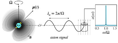
Figure 1: A neutron star (NS) rotating with frequency $\Omega$ emits axions from gap regions where $\textbf{E}\cdot\textbf{B}\neq 0$ (shown in grey for the VDM model and in yellow for the PC model, not to scale). Relativistic axions emitted by the NS may convert to detectable signals in laboratory experiments (pulsarscopes). The resulting signal is highly coherent, with a prominent peak in frequency at the pulsar rotation frequency, $\Omega$.

Axion Radiation from Pulsars.— The axion field sourced by a pulsar is determined by the distribution of ${\bf E}\cdot{\bf B}$ in the magnetosphere according to the Klein-Gordon equation, $(\Box+m_{a}^{2})a(x)=g_{a\gamma\gamma}{\bf E}\cdot{\bf B}$. In the limit where the axion mass $m_{a}\to 0$, this equation is analogous to that for the electric potential, interpreted as $a(x)$, in Lorenz gauge with charge density $\rho_{\rm eff}=g_{a\gamma\gamma}{\bf E}\cdot{\bf B}$. Thus, one can calculate the radiated axion signal given a model for ${\bf E}\cdot{\bf B}$ exterior to a NS.

We consider two limiting scenarios for ${\bf E}\cdot{\bf B}$. The first is the Vacuum Dipole Model (VDM) Deutsch (1955); Hoyle et al. (1964); Pacini (1967, 1968); Ostriker and Gunn (1969); Melrose and Yuen (2012). In this case, the exterior of the NS is assumed to be vacuum and the magnetic field is described by a rotating dipole with magnetic moment $\bm{\mu}(t)=B_{0}R_{\rm NS}^{3}{\hat{\mu}}(t)$, where $B_{0}$ is the surface magnetic field and $R_{\rm NS}$ the NS radius. The unit vector $\hat{\mu}$ is misaligned from the rotation axis by an angle $\theta_{m}$ and rotates around the axis with frequency $\Omega$. The NS is well-approximated as a perfect conductor, therefore ${\bf E}\cdot{\bf B}=0$ in the interior. The exterior ${\bf E}\cdot{\bf B}$ is determined by solving Laplace’s equation with conducting boundary conditions imposed on the NS surface Deutsch (1955).

In the VDM, it follows that

$$\begin{split}{\bf E}\cdot{\bf B}={|\bm{\mu}|^{2}\Omega\over 4r^{5}}&\left[\cos\theta\sin^{2}\theta_{m}+{1\over 2}\sin\theta\sin{(2\theta_{m})}\times\right.\\ &\left.\big{(}\Omega r\cos(\phi-\Omega t)-\sin(\phi-\Omega t)\big{)}\right]\,,\end{split}$$ (1)

with $(\theta,\phi)$ the spherical coordinates in the frame in which $\hat{z}$ is aligned with the NS’s rotation axis. The first term on the right-hand-side of (1) does not have time dependence and thus does not radiate axions, while the second term gives sub-dominant radiated power relative to the third by an amount proportional to $\Omega R_{\rm NS}\ll 1$. The third term in (1) shows that the radiation will be at angular frequency $\Omega$ with dipole moment

$$\begin{split}|{\bf p}_{\rm eff}|=\left|\int d^{3}x\,{\bf x}\rho_{\rm eff}({\bf x})\right|\approx{\pi\over 6}g_{a\gamma\gamma}{|\bm{\mu}|^{2}\Omega\over R_{\rm NS}}\sin(2\theta_{m})\,.\end{split}$$ (2)

Using the dipole radiation formula, this suggests a radiated power in axions of the form

$$\begin{split}P_{a}&\approx{\pi\over 432}g_{a\gamma\gamma}^{2}B_{0}^{4}\Omega^{6}R_{\rm NS}^{10}\sin^{2}(2\theta_{m})\\ &\approx 1.4\times 10^{35}\,\,{{\rm erg}\over{\rm s}}\left({g_{a\gamma\gamma}\over 10^{-12}\,\,{\rm GeV}^{-1}}\right)^{2}\left({\Omega\over 2\pi\times 30\,\,{\rm Hz}}\right)^{6}\\ &\times\left({{R_{\rm NS}}\over 14\,\,{\rm km}}\right)^{10}\left({B_{0}\over 8.5\times 10^{12}\,\,{\rm G}}\right)^{4}\sin^{2}(2\theta_{m})\,.\end{split}$$ (3)

The fiducial pulsar parameters above correspond to those of the Crab pulsar, as motivated below. The Supplementary Material (SM) generalizes (3) to include the non-zero axion mass (see also Garbrecht and McDonald (2018)).

For sufficiently rapid pulsar rotation, ${\bf E}\cdot{\bf B}$ is strong enough to liberate charges from the NS surface, which populate the magnetosphere and screen the electric field in the process. However, even in active pulsars, ${\bf E}\cdot{\bf B}$ is not expected to be screened everywhere. An example of a partially-screened magnetosphere is the disk-dome or electrosphere solution found in slowly-rotating NSs Pétri et al. (2002); Philippov and Kramer (2022); Cruz et al. (2023). These solutions have screened magnetospheres extending out to distances of order $R_{\rm NS}$ from the NS surface, beyond which the VDM applies. Referring to (2), excluding distances up to $xR_{\rm NS}$ from the NS center, with $x\sim$ few, reduces the radiated power by a factor of $x$.

A lower bound on the axion emission power may be computed assuming the magnetosphere is mostly screened. The production of screening $e^{\pm}$ pairs occurs in gap regions with non-vanishing ${\bf E}\cdot{\bf B}$, such as those that arise near the magnetic poles of the pulsar. Pulsar rotation defines a boundary, called the light cylinder (at radius $R_{\rm LC}=1/\Omega$ in natural units), beyond which particles cannot co-rotate with the NS. Charged particles escape the magnetosphere along open field lines (defined as those that do not close within the light cylinder), leading to charge starvation above the polar cap (PC), defined as the region on the NS surface that contains the footpoints of all open field lines. The dearth of plasma above the PC opens a gap with ${\bf E}\cdot{\bf B}\neq 0$. As the gap grows, it becomes unstable to runaway $e^{\pm}$ pair production, the dynamics of which have been modeled semi-analytically in Tolman et al. (2022); Noordhuis et al. (2023) and from first-principles kinetic plasma simulations in Cruz et al. (2021, 2022). All timescales associated with screening of the electric field are much smaller than the rotational period of the pulsar. Thus, when considering axion radiation at the rotational frequency, the gap may be treated as a point particle with “axion charge”

$$Q_{a}=g_{a\gamma\gamma}\displaystyle\int_{\rm gap}d^{3}x\left\langle{\bf E}\cdot{\bf B}({\bf x},t)\right\rangle_{t}\,,$$ (4)

where $\left\langle.\right\rangle_{t}$ represents the time average. We assume that the gap is screened for one light crossing time and model the gap as a cylinder with radius $r_{\scriptscriptstyle{\rm PC}}=R_{\rm NS}\sqrt{\Omega R_{\rm NS}}$ and height $h$. Note that the gap radius may be derived by equating the magnetic flux through the PC region, $\pi B_{0}r_{\scriptscriptstyle{\rm PC}}^{2}$, and the flux through the light cylinder Goldreich and Julian (1969). At low altitude, $\ell\ll R_{\rm NS}$ with $\ell$ the height above the NS surface, the electric field in the gap is $E_{\parallel}(\ell)=2\Omega B_{0}\ell$, which corresponds to a voltage drop across the gap of $\Phi_{{\scriptscriptstyle{\rm PC}}}=\Omega B_{0}h^{2}$ Ruderman and Sutherland (1975). With this geometry, the axion charge is $Q_{a}=\pi g_{a\gamma\gamma}B_{0}^{2}\Omega r_{\scriptscriptstyle{\rm PC}}^{2}h^{2}$.

The height of the gap is limited by the vacuum breakdown; as $h$ increases, the voltage drop increases and the gap becomes unstable to pair production. Most conservatively, we may set $h$ to be the mean free path of a pair-producing photon Timokhin and Harding (2015, 2019); Caputo et al. (2023), which is approximated by Ruderman and Sutherland (1975)

$$\begin{split}h\sim 7\,\,{\rm m}\left({\Omega\over 2\pi\times 30\,\,\,{\rm Hz}}{B_{0}\over 8.5\times 10^{12}\,\,{\rm G}}\right)^{-4/7}\,.\end{split}$$ (5)

The true gap height may be larger than that in (5) by a factor $N_{\rm gen}$, which represents the number of generations of pair production required to screen the gap. Assuming the charge density grows exponentially during the cascade, $N_{\rm gen}$ depends logarithmically on the ratio between the current supplied by the magnetosphere and the Goldreich-Julian current density $j_{\rm GJ}\sim 2\Omega B_{0}$, giving $N_{\rm gen}\sim$ few. Modeling the current supply of the magnetosphere requires global simulations, and so we assume $N_{\rm gen}=1$ in this work to be conservative.

A NS with a dipole magnetic field has two antipodal PCs with opposite “axion charge.” Taking the model of two oppositely charged point masses rotating rigidly and inclined at an angle $\theta_{m}$ relative to the rotation axis, the radiated power in the dipole approximation is

$$\begin{split}P_{a}&\approx{{1\over 3\pi}}R_{\rm NS}^{2}\Omega^{4}Q_{a}^{2}\sin^{2}\theta_{m}\\ &\approx{10^{20}}\,\,{{\rm erg}\over{\rm s}}\left({g_{a\gamma\gamma}\over 10^{-12}\,\,{\rm GeV}^{-1}}\right)^{2}\left({\Omega\over 2\pi\times 30\,\,{\rm Hz}}\right)^{{40\over 7}}\\ &\times\left({{R_{\rm NS}}\over 14\,\,{\rm km}}\right)^{8}\left({B_{0}\over 8.5\times 10^{12}\,\,{\rm G}}\right)^{12/7}\sin^{2}(\theta_{m})\,,\end{split}$$ (6)

for $m_{a}\ll\Omega$. See SM for the generalization to non-zero axion mass. Equations (3) and (6) fully bracket the current uncertainties on the emitted power in axions.

Among pulsars in the ATNF catalog Manchester et al. (2005), the Crab pulsar provides the highest axion power, by a factor of $\approx 20$ in the VDM, and is within a factor of two of the most efficient axion-emitting pulsar in the PC model. The spin-down parameters of the Crab are measured directly from timing of the radio beam: $P=0.0338238880741$ s ($\Omega/2\pi=29.5649038871$ Hz) and $\dot{P}=4.1958812\times 10^{-13}$ (on 15/1/2024) Lyne et al. (1993); Manchester et al. (2005). Its radius, $R_{\rm Crab}$, may be determined by observations of the Crab nebula Bejger and Haensel (2002): $R_{\rm Crab}=14$–$15$ km, where the spread arises due to uncertainty in the NS equation of state. Self-consistently incorporating the measurement of the pulsar radius, mass, and moment of inertia with the equation for vacuum-filled pulsar spin down gives $B_{\rm Crab}>8.5~{}(6.9)\times 10^{12}$ G for $R_{\rm Crab}=14$ ($15$) km Philippov et al. (2014). These inferred magnetic field values are roughly consistent with those from analytic spin-down models studied in Kou and Tong (2015), $B_{\rm Crab}=(5.0$–$8.3)\times 10^{12}$ G. Motivated by these analyses, we fix the relevant Crab pulsar parameters to be $R_{\rm NS}=14$ km and $B_{0}=8.5\times 10^{12}$ G, which are conservative within the aforementioned observational constraints.

Detecting Pulsar-Sourced Axions.— The pulsar-induced axion field $a({\bf x},t)$ on Earth is analogous to that of DM (see, e.g., Foster et al. (2018)) with a few exceptions. First, the local energy density in axions due to the pulsar is given by $\rho_{{}_{\rm PS}}=P_{a}/(4\pi D^{2})$, with $D$ the distance to the pulsar. The terrestrial energy density of pulsar-sourced axions, $\rho_{{}_{\rm PS}}$, is in general much less than the local DM density, $\rho_{{}_{\rm DM}}$. For example, if the full spin-down power of the Crab pulsar were emitted in axions, the ratio of energy densities would be $\rho_{{}_{\rm PS}}/\rho_{{}_{\rm DM}}\sim 10^{-13}$. Despite the orders-of-magnitude suppression in the local axion density, pulsar-sourced axions possess several key differences relative to DM axions that facilitate their detection.

While DM axions are non-relativistic, with characteristic momenta $k\sim 10^{-3}\omega$ and $\omega\sim m_{a}$, pulsar-induced axions are generically relativistic, with $k=\sqrt{\omega^{2}-m_{a}^{2}}\sim\omega$ for $m_{a}\ll\omega\approx\Omega$. (Note that axions are only produced by the pulsar if $m_{a}<\Omega$.) This aspect of the pulsar-induced axion signal is useful for experiments such as CASPEr-wind that rely on the axion field’s spatial gradient.

DM axions are expected to be ultra-narrow in frequency space, with the axion field only having non-trivial support over a spread in frequencies $\delta\omega/\omega\sim 10^{-6}$, but the pulsar-induced axion signals may be even narrower. Assuming that the un-screened parts of magnetosphere co-rotate with the NS, then the axion signal has a natural line width set by the pulsar spin-down parameters: $\delta\omega/\omega=\dot{P}$, where $\dot{P}$ is the observed rate of change of the period. Most observed pulsars have $\dot{P}\ll 10^{-10}$, giving nearly monochromatic axion signals. For example, the Crab pulsar has $\dot{P}\approx 4.2\times 10^{-13}$ as mentioned previously, making the Crab-induced axion signal millions of times narrower than the expected DM signal. (Note that every few years the Crab undergoes small sporadic “glitches,” resulting in changes in the frequency and amplitude of the signal; we assume the observing window does not contain any such major timing anomalies.) By causality, deviations from co-rotation are expected near the light cylinder. On the other hand, in both the VDM model and the PC model, along with the electrosphere model, the axion emission is predominantly produced near the NS surface and far from the light cylinder. Understanding the extent to which magnetosphere drag may affect the signal line width requires dedicated simulations that include general relativistic effects, which are beyond the scope of this work.

Another key aspect of the pulsar-induced axion signal is that it is generated at known frequencies, unlike in the case of DM. Given that the mass of the DM axion is currently unknown, experiments must scan over millions of different possibilities. On the other hand, the Crab signal is at the known frequency $f\approx 29.6$ Hz. The frequency of the signal is modulated by known effects (e.g. pulsar spin down and motion of the Earth), requiring real-time adjustment of the observing frequency.

We now follow the formalism in Foster et al. (2018); Dror et al. (2021) to project the sensitivity of key upcoming axion DM experiments to the signal from the Crab pulsar. We concentrate on experiments like Dark SRF and CASPEr-wind, though in the SM we discuss DMRadio-GUT, which may yield comparable sensitivity relative to a Dark SRF experiment.

Superconducting radio frequency (SRF) cavities have demonstrated quality factors $Q\gtrsim 10^{11}$ Romanenko et al. (2014); Posen et al. (2019), making them ideal resonators to look for highly monochromatic axion signals. The Dark SRF approach (called “heterodyne detection”) to low-frequency axion detection involves the axion driving a transition between two nearly degenerate modes of an SRF cavity Berlin et al. (2020, 2021). In this approach, the axion field drives a transition from a cavity “pump mode” of frequency $\omega_{0}\sim$ GHz to a nearly-degenerate “signal mode” of frequency $\omega_{1}\approx\omega_{0}+\omega_{a}$, where $\omega_{a}$ is the frequency of the axion field. The signal is measured by a readout waveguide coupled to the signal mode Berlin et al. (2020, 2021).

We envision measuring the power in the signal mode at equal time intervals over a total integration time $t$ and then computing the power spectral density (PSD) of the data in frequency space. Since the axion coherence time ($\tau_{a}\gtrsim$ kyr) is much larger than $t$, the axion signal is expected to lie entirely in a single frequency bin, labeled $k^{*}$. The power in bin $k^{*}$, obtained by integrating the PSD over the bin (see SM for details), is

$$S_{k^{*}}\simeq\pi^{2}\left(g_{a\gamma\gamma}\eta_{10}B_{p}\right)^{2}V_{\rm cav}\left({Q_{1}\over\omega_{1}}\right){\rho_{{}_{\rm PS}}}\,,$$ (7)

where $\eta_{10}$ is a dimensionless mode overlap factor, $B_{p}$ is the magnetic field amplitude of the pump mode, $V_{\rm cav}$ is the cavity volume, and $Q_{1}$ is the loaded quality factor of the signal mode. At the Crab pulsar frequency, the dominant noise source is thermal. The noise power in bin $k^{*}$ is (see SM)

$$B_{k^{*}} \simeq 4\pi T_{\rm cav}\left({Q_{1}\over Q_{\rm int}}\right)\Delta\omega\,,$$ (8)

where $T_{\rm cav}$ is the cavity temperature, $Q_{\rm int}$ is the intrinsic quality factor of the cavity, and $\Delta\omega=2\pi/t$ is the frequency bin width. The probability of observing a given PSD in bin $k^{*}$ is exponentially distributed with mean $S_{k^{*}}+B_{k^{*}}$ for fixed signal parameters; this implies that the expected 95% upper limit under the null hypothesis may be determined by setting $S_{k^{*}}/B_{k^{*}}\approx 8.48$ Dror et al. (2023). Figure 2 (left panel) shows this projection, adopting fiducial parameters for the Crab pulsar as described previously and fiducial detector parameters: $\eta_{10}=1$, $B_{p}=0.2$ T, $V_{\rm cav}=1\ {\rm m}^{3}$, $\omega_{0}\approx\omega_{1}=2\pi\times 100$ MHz, $Q_{\rm int}\approx Q_{1}\approx 10^{12}$, $T_{\rm cav}=1.8$ K, and $t=1$ year as in Berlin et al. (2020, 2021).

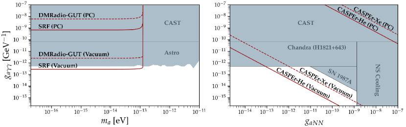
Figure 2: Left: The projected sensitivity to the axion-photon coupling $g_{a\gamma\gamma}$ as a function of the axion mass, $m_{a}$, from one-year dedicated searches with the proposed Dark SRF axion experiment and the DMRadio-GUT experiment for the axion-induced signal from the Crab pulsar at $f\approx 29.6$ Hz. We illustrate projected 95% upper limits under the null hypothesis assuming both the VDM magnetosphere (‘Vacuum’) and for the PC model, where the axions are only produced in small gaps near the NS poles. The grey shaded regions represent current constraints on this parameter space, as summarized in the main text. Right: As in the left panel, but for the future CASPER-wind experiment, which searches for the axion-nucleon coupling $g_{aNN}$. This figure assumes $m_{a}\ll 10^{-13}$ eV and illustrates the projected 95% upper limits in the $g_{a\gamma\gamma}-g_{aNN}$ plane, for two different target materials.

Figure 2 (left panel) compares the expected sensitivity to existing constraints from the CAST experiment Arik et al. (2015), which looks for axions produced in the Sun. The shaded grey region also illustrates the current constraints from a number of astrophysical axion probes, including searches for spectral distortions of astrophysical sources with Chandra X-ray data Reynés et al. (2021); Reynolds et al. (2020); Marsh et al. (2017); Wouters and Brun (2013) and super star cluster searches for axions with NuSTAR X-ray data Dessert et al. (2020). Note that some of the astrophysical limits shown may also be subject to theoretical uncertainties (e.g., Libanov and Troitsky (2020); Matthews et al. (2022)). Assuming the VDM (labeled ‘Vacuum’), the Dark SRF projected sensitivity would be world leading, improving upon the CAST bounds on $g_{a\gamma\gamma}$ by more than two orders of magnitude. In the electrosphere model, the axion power is lower than predicted by the VDM by a factor of $x\sim$ few, which leads to a modest drop in sensitivity of $x^{1/4}$. Assuming the conservative PC model, with radiated power given in (6), the projected sensitivity does not pass that of the CAST experiment. This motivates more detailed modeling of the Crab pulsar magnetosphere to determine precisely where the sensitivity lies.

Figure 2 (left panel) also illustrates the projected sensitivity of the planned DMRadio-GUT experiment Brouwer et al. (2022b), assuming the experiment takes data with a quality factor of $2\times 10^{7}$ Brouwer et al. (2022b) for one year with a resonant readout at the Crab frequency. See the SM for further details.

The right panel of Fig. 2 shows the projected sensitivity of the CASPEr-wind experiment Budker et al. (2014); Jackson Kimball et al. (2020); Garcon et al. (2019); Wu et al. (2019) under both the VDM and PC magnetosphere models, assuming $m_{a}\ll 10^{-13}$ eV. CASPEr-wind searches for the axion through its coupling to the nucleon: $H_{\rm int}=\gamma_{N}{\bm{B}}_{a}\cdot{\bm{S}}_{N}$, with $\gamma_{N}$ the nucleon gyromagnetic ratio and ${\bm{B}}_{a}$ an effective magnetic field that is equal to ${\bm{B}}_{a}=-g_{aNN}{\bm{\nabla}}a/\gamma_{N}$. CASPEr-wind, and also co-magnetometer experiments such as Lee et al. (2023); Bloch et al. (2022), use nuclear magnetic resonance techniques with a transverse magnetometer to search for spin precession of a magnetized sample due to the axion interaction Hamiltonian; the effect is resonantly enhanced when the axion frequency matches the Larmor frequency $\omega_{0}=\gamma_{N}B_{E}$, with $B_{E}$ the static external magnetic field that aligns the spins.

Measuring the transverse magnetic field over $t=1\,\,{\rm year}$, the axion signal contributes to a single frequency bin because $t\ll\tau_{a}$. On the other hand, the width of the resonance is limited by the transverse spin relaxation time $T_{2}$, which is expected to be much less than $t$. As in the SRF case, one may compute the expected signal contribution within the frequency bin $k^{*}$ and compare it to the expected background noise, which arises predominantly from spin projection and magnetometer noise for CASPEr-wind Dror et al. (2023). (See the SM for details.)

Figure 2 (right panel) shows the projected 95% upper limits in the space of $|g_{a\gamma\gamma}|$ and $|g_{aNN}|$. (Note that the observed signal is proportional to the combination $g_{a\gamma\gamma}^{2}g_{aNN}^{2}$.) The projected sensitivity is shown for two different assumptions regarding the CASPEr-wind type experiment (see, e.g., Dror et al. (2023) for the justification of these choices): the more conservative case takes a Xe-129 target, which has a nuclear magnetic moment of $0.78\mu_{N}$, with $\mu_{N}$ the nuclear magneton, along with the number density $n\approx 1.3\times 10^{22}$ cm^-3. The more optimistic scenario assumes a Helium-3 target with a nuclear magnetic moment $\sim$$2.1\mu_{N}$ and $n\approx 2.8\times 10^{22}$ cm^-3. For both, the volume is $1$ m³, spin relaxation time is $T_{2}=100$ sec, and the effective SQUID loop area is $0.3\ {\rm cm}^{2}$.

We compare the expected upper limits from CASPEr-wind to the existing constraints on this parameter space on $g_{a\gamma\gamma}$ alone along with the NS cooling constraints on $g_{aNN}$ Buschmann et al. (2022). Additionally, the non-observation of gamma-rays from SN1987A that would have been produced by nucleon bremsstrahlung (with $g_{aNN}$) and then converted to gamma-rays in the Galactic magnetic fields (with $g_{a\gamma\gamma}$) gives a constraint on the combination $g_{a\gamma\gamma}\times g_{aNN}$ Payez et al. (2015); Manzari et al. (pear), which is also illustrated. Both the Xe and He targets could probe previously unexplored regions of parameter space for the VDM magnetosphere.

Discussion.— We proposed a new target for axion DM detection experiments: pulsar-sourced axions. These relativistic axions are produced at known frequencies; for example, the signal from the Crab pulsar is around $f\approx 29.6$ Hz. Upcoming searches for axions from the Crab pulsar may probe previously-unexplored regions of low-mass axion parameter space. Global particle-in-cell (PIC) plasma simulations of the Crab magnetosphere along the lines of Spitkovsky (2006); Kalapotharakos and Contopoulos (2009); Pétri (2012) are needed to better model the distribution of ${\bf E}\cdot{\bf B}$ in the magnetosphere and compute the axion luminosity and line width more accurately.

It is also possible that better pulsar candidates exist that are not known at present. These could include high-field, high-period pulsars that are not beamed towards Earth or are otherwise obscured to electromagnetic radiation. Young pulsars born after supernova, including possible future supernova, may also be superior targets. Transient axion signals could also arise from gamma-ray bursts and magnetar glitches.

The axion emission from pulsars may also directly affect the observed pulsar quantities such as the period and magnetic field. For example, the spin-down luminosity of the Crab pulsar is $L_{\rm spin-down}=4.5\times 10^{38}$ erg/s Manchester et al. (2005). The axion-induced emission formula in (3) surpasses the spin-down luminosity for axion-photon couplings larger than $g_{a\gamma\gamma}\sim 5\times 10^{-11}$ GeV^-1. This strongly suggests a conservative upper limit of $|g_{a\gamma\gamma}|\lesssim 5\times 10^{-11}$ GeV^-1, assuming the VDM model, for $m_{a}\lesssim 10^{-13}$ eV. On the other hand, the limit can likely be substantially improved by studying the back-reaction of the axion emission more carefully on the pulsar dynamics.

Another class of astrophysically-produced low-frequency axions that could be detectable with terrestrial DM detectors are signals narrow in the time domain. For example, we estimate that NS-NS inspirals and NS-black-hole inspirals may yield detectable but short-lived axion signals, which would be coincident in time with gravitational wave signals, depending on the magnetic properties of the NSs and the distance to the event. We leave detailed estimates of this signal to future work, which could most optimistically add axions as an additional messenger to the growing field of multi-messenger astronomy.

Acknowledgments— The authors acknowledge A. Berlin, S. Chaudhuri, J. Foster, H.  Hakobyan, Y. Kahn, N. Rodd, A. Sushkov, L. Winslow, and S. Witte for helpful discussions. ML and MK are supported by the Department of Energy (DOE) under Award Number DE-SC0007968. ML also acknowledges support from the Simons Investigator in Physics Award. AP acknowledges support from the Princeton Center for Theoretical Science. BRS is supported in part by the DOE Early Career Grant DESC0019225 and in part by a Sloan Research Fellowship. MK is grateful to Princeton University for their hospitality. The work presented in this paper was performed on computational resources managed and supported by Princeton Research Computing. This research also made extensive use of the publicly available codes IPython (Pérez and Granger, 2007), matplotlib (Hunter, 2007), Jupyter (Kluyver et al., 2016), NumPy (Harris et al., 2020), and SciPy (Virtanen et al., 2020).

Supplementary Material for An Axion Pulsarscope
Mariia Khelashvili, Mariangela Lisanti, Anirudh Prabhu, and Benjamin R. Safdi

I Axion Emission in a Pulsar’s Electromagnetic Field

The derivation of the axion power in the vacuum dipole model (VDM) and the polar cap (PC) model in the main text assumes the axion is massless. This section generalizes the derivation to finite mass $m_{a}\leq\Omega$, where $\Omega$ is the pulsar’s rotational frequency. The evolution of the axion field exterior to the pulsar is governed by the Klein-Gordon equation, $(\Box+m_{a}^{2})a(x)=g_{a\gamma\gamma}{\bf E}\cdot{\bf B}$, where ${\bf E}$ (${\bf B}$) is the electric (magnetic) field in the pulsar magnetosphere. The Klein-Gordon equation with a source can be solved using the retarded Green function (Bogolyubov and Shirkov, 1959; Economou, 2006):

$$G(\mathbb{x},\tau)=\frac{\theta(\tau)}{2\pi}\left(\delta(s^{2})-\frac{m_{a}}{2s}\theta(s^{2})\,J_{1}(m_{a}s)\right)\,,\qquad s^{2}=\tau^{2}-\mathbb{x}^{2}\,\,,$$ (S1)

where $J_{1}(x)$ is the Bessel function, $\theta$ is the Heaviside function, and $\delta$ is the delta function. The solution can be simplified for the case of localized periodic sources using the method of (Li and Ruffini, 1986; Krause et al., 1994). In this case, the radiation from the pulsar magnetosphere is sourced by the dipole moment of ${\bf E}\cdot{\bf B}$ to leading-order (see, e.g., (2) in the main text). We briefly summarize the calculations of axion dipole radiation and then apply the results to the two magnetosphere models considered in this work.

Assuming that the source periodically rotates at the pulsar rotation frequency $\Omega$, the axion-field solution takes the form Krause et al. (1994)

$$a(\mathbf{r},t)=\sum\limits_{m=-\infty}^{\infty}e^{-im\Omega t}a_{m}(\mathbf{r})\,.$$ (S2)

In general, periodically rotating sources radiate at the fundamental frequency $\Omega$ and its integer multiples. For any realistic pulsar, however, the near-surface region rotates with velocity $v\sim\Omega R_{\rm NS}\ll 1$, where $R_{\rm NS}$ is the neutron star’s radius, and radiated power at higher frequencies is highly suppressed compared to the fundamental frequency by powers of $v$. Thus, we only consider radiation at the fundamental frequency:

$$a(\mathbf{r},t)=e^{-i\Omega t}a_{\scriptscriptstyle{\Omega}}(\mathbf{r})+e^{i\Omega t}a_{\scriptscriptstyle{-\Omega}}(\mathbf{r})\,.$$ (S3)

The corresponding Fourier component of the charge density, $\rho_{\rm eff}(\mathbf{r},t)\equiv g_{a\gamma\gamma}{{\bf E}\cdot{\bf B}}(\mathbf{r},t)$, is

$$\rho_{\scriptscriptstyle{\pm\Omega}}(\mathbf{r})=\frac{1}{T}\int\limits_{0}^{T}dt\,e^{\pm i\Omega t}\rho_{\rm eff}(\mathbf{r},t)\,,$$ (S4)

where $T=2\pi/\Omega$ is the source rotation period. The axion field obeys the equation of motion:

$$(\nabla^{2}+k^{2})a_{\scriptscriptstyle{\pm\Omega}}(\mathbf{r})=-\rho_{\scriptscriptstyle{\pm\Omega}}(\mathbf{r})\,,\quad k=\sqrt{\Omega^{2}-m_{a}^{2}}\,.$$ (S5)

We may solve this equation using the outgoing-wave Green function Krause et al. (1994),

$$G(\mathbf{r},\mathbf{r}^{\prime})=\frac{1}{4\pi}\frac{e^{\pm ik|\mathbf{r}-\mathbf{r}^{\prime}|}}{|\mathbf{r}-\mathbf{r}^{\prime}|}\,,$$ (S6)

leading to

$$a_{\scriptscriptstyle{\pm\Omega}}(\mathbf{r})=\frac{1}{4\pi}\int d^{3}r^{\prime}\frac{e^{\pm ik|\mathbf{r}-\mathbf{r}^{\prime}|}}{|\mathbf{r}-\mathbf{r}^{\prime}|}\rho_{\scriptscriptstyle{\pm\Omega}}(\mathbf{r}^{\prime})\,.$$ (S7)

In the long-wavelength ($k|\mathbf{r}^{\prime}|\ll 1$), far-field ($|\mathbf{r}|\gg|\mathbf{r}^{\prime}|$) limit, the solution takes the form

$$a_{\scriptscriptstyle{\pm\Omega}}(\mathbf{r})=\frac{e^{\pm ikr}}{4\pi r}\left(\int d^{3}r^{\prime}\rho_{\scriptscriptstyle{\pm\Omega}}(\mathbf{r}^{\prime})\pm ik\hat{n}\cdot\int d^{3}r^{\prime}\rho_{\scriptscriptstyle{\pm\Omega}}(\mathbf{r}^{\prime})\mathbf{r}^{\prime}+\cdots\right)=\frac{e^{\pm ikr}}{4\pi r}\left[Q_{\scriptscriptstyle{\pm\Omega}}\pm ik\hat{n}\cdot\mathbf{p}_{\scriptscriptstyle{\pm\Omega}}+\cdots\right]\,,$$ (S8)

where $\hat{n}$ is the unit vector in the direction of $\mathbf{r}$, and $Q_{\scriptscriptstyle{\pm\Omega}}$ ($\mathbf{p}_{\scriptscriptstyle{\pm\Omega}}$) is the monopole (dipole) moment of $\rho_{\scriptscriptstyle{\pm\Omega}}$, given by

$$Q_{\scriptscriptstyle{\pm\Omega}}=\int d^{3}r^{\prime}\rho_{\scriptscriptstyle{\pm\Omega}}(\mathbf{r}^{\prime})\,,\qquad\mathbf{p}_{\scriptscriptstyle{\pm\Omega}}=\int d^{3}r^{\prime}\rho_{\scriptscriptstyle{\pm\Omega}}(\mathbf{r}^{\prime})\mathbf{r}^{\prime}\,.$$ (S9)

In the VDM and PC models, the monopole term vanishes and the leading-order term is that of the dipole. The time-dependent solution for the outgoing axion wave radiated by the dipole is

$$a(\mathbf{r},t)=\frac{ik}{4\pi r}\left(\hat{n}\cdot\mathbf{p}_{\scriptscriptstyle{+\Omega}}\,e^{-i(\Omega t-kr)}-\hat{n}\cdot\mathbf{p}_{\scriptscriptstyle{-\Omega}}\,e^{i(\Omega t-kr)}\right)\,.$$ (S10)

The radiated axion power follows:

$$P_{a}=\int\bm{\Pi}\cdot d\bm{\sigma}\,,\qquad\langle\bm{\Pi}\rangle_{T}=\langle\dot{a}^{*}\bm{\nabla}a\rangle_{T}=\langle\dot{a}_{\scriptscriptstyle{\Omega}}^{*}(\mathbf{r},t)\bm{\nabla}a_{\scriptscriptstyle{\Omega}}(\mathbf{r},t)+\dot{a}_{\scriptscriptstyle{-\Omega}}^{*}(\mathbf{r},t)\bm{\nabla}a_{\scriptscriptstyle{-\Omega}}(\mathbf{r},t)\rangle_{T}\,,$$ (S11)

where $\left\langle..\right\rangle_{T}$ represents the time-average over the rotational period. For a real source, $\operatorname{Im}\rho(\mathbf{r},t)=0$ and the Fourier components are $\rho_{{\scriptscriptstyle{-\Omega}}}^{*}=\rho_{{\scriptscriptstyle{\Omega}}}$, therefore $\mathbf{p}_{-\scriptscriptstyle{\Omega}}^{*}=\mathbf{p}_{\scriptscriptstyle{\Omega}}$ and the total axion dipole radiation becomes:

$$\langle P_{a}\rangle_{T}=\frac{1}{8\pi^{2}}\Omega k^{3}\iint d\omega_{n}|\mathbf{p}_{\scriptscriptstyle{\Omega}}\cdot\hat{n}|^{2}\,.$$ (S12)

The integration is performed over the solid angle $\omega_{n}$, and the final expression includes the Fourier component of the dipole moment:

$$\mathbf{p}_{\scriptscriptstyle{\Omega}}=\frac{1}{T}\int\limits_{0}^{T}dt\,e^{i\Omega t}\int d^{3}r\rho_{\rm eff}(\mathbf{r},t)\mathbf{r}\,.$$ (S13)

I.1 Vacuum Dipole Model

For a fully unscreened magnetosphere, the distribution of effective charge density, $g_{a\gamma\gamma}{\bf E}\cdot{\bf B}$, in the pulsar’s magnetosphere is given by (1). The radiation of axions in this scenario can be modeled by a rotating dipole with effective dipole moment (2). From (S13),

$$\hat{n}\cdot\mathbf{p}_{\scriptscriptstyle{\Omega}}\approx\frac{i\pi}{12}g_{a\gamma\gamma}\frac{|\bm{\mu}|^{2}\Omega}{R_{\rm NS}}\sin(2\theta_{m})\sin\theta_{n}e^{i\phi_{n}}\,,$$ (S14)

where $|\bm{\mu}|=B_{0}R_{\rm NS}^{3}$, $B_{0}$ is the surface magnetic field of the pulsar, $\theta_{m}$ is the angle between the pulsar’s magnetic dipole axis and its rotation axis, and $(\theta_{n},\phi_{n})$ are the angles in spherical coordinates that define the direction of $\hat{n}$. From the dipole radiation power (S12), it follows that

$$\langle P_{a}\rangle_{T}=\frac{\pi}{432}g_{a\gamma\gamma}^{2}B_{0}^{4}\Omega^{6}R_{\rm NS}^{10}\sin^{2}(2\theta_{m})\left(1-\frac{m_{a}^{2}}{\Omega^{2}}\right)^{3/2}\,,$$ (S15)

which reduces to (3) in the limit of a massless axion.

I.2 Polar Cap Model

We now discuss the model of a mostly-screened magnetosphere, where the axion is sourced only in the small polar cap (PC) regions above the magnetic poles. The size of the PC, $r_{\text{pc}}\ll R_{\rm NS}\ll 1/\Omega$, can be neglected, so we model the PCs as two rotating point-like sources with opposite charges ($Q_{a}^{N}=-Q_{a}^{S}$) and opposite velocity and position ($\mathbb{v}_{\rm pc}^{N}=-\mathbb{v}_{\rm pc}^{S}$ and $\mathbb{r}_{\rm pc}^{N}=-\mathbb{r}_{\rm pc}^{S}=\mathbf{q}(t)$), where $N$ ($S$) represents the PC at the northern (southern) pole. The effective charge density for the point-like PC model is

$$\rho(\mathbf{r},t)=Q_{a}\left[\delta(\mathbf{r}-\mathbf{q}(t))-\delta(\mathbf{r}+\mathbf{q}(t))\right]\,,$$ (S16)

where

$$\mathbf{q}(t)=R_{\rm NS}\left(\sin\theta_{m}\left(\cos(\Omega t)\hat{\bf x}+\sin(\Omega t)\hat{\bf y}\right)+\cos\theta_{m}\hat{\bf z}\right)\,.$$ (S17)

We can find the Fourier component of the dipole moment (S13):

$$\hat{n}\cdot\mathbf{p}_{\scriptscriptstyle{\Omega}}=Q_{a}R_{\rm NS}\sin\theta_{m}\sin\theta_{n}e^{-i\phi_{n}}\,,$$ (S18)

where $\theta_{n},\phi_{n}$ are spherical coordinate angles of the observer. Finally, the resulting axion radiation power is:

$$\langle P_{a}\rangle_{T}=\frac{1}{3\pi}R_{\rm NS}^{2}\Omega^{4}Q_{a}^{2}\sin^{2}\theta_{m}\left(1-\frac{m_{a}^{2}}{\Omega^{2}}\right)^{3/2}\,,$$ (S19)

which is the same as (6) in the ultra-relativistic limit ($m_{a}\ll\Omega$).

II Dark SRF Projection

This section provides details for computing the sensitivity of superconducting radio frequency (SRF) cavities to relativistic monochromatic axion signals, using the conventions described in Berlin et al. (2020, 2021). The search for relativistic axions does not exactly map onto the search for non-relativistic axion DM, since spatial gradients cannot be ignored in the former case. In particular, the wave equation takes the form

$$\left({\partial^{2}\over\partial t^{2}}-\bm{\nabla}^{2}\right){\bf E}=g_{a\gamma\gamma}\left((\bm{\nabla}a\cdot\bm{\nabla}){\bf B}_{p}-\dot{a}{\partial{\bf B}_{p}\over\partial t}\right)\,,$$ (S20)

where $a$ is the axion field and ${\bf B}_{p}$ is the magnetic field associated with the pump mode. The first term on the right-hand side in (S20) can be neglected as it is incapable of exciting resonant modes of a cavity Dror et al. (2021). The axion field drives power into the signal mode, with the following power spectral density (PSD) (see e.g., Berlin et al. (2020)):

$$S_{\rm sig}(\omega) ={\omega_{1}\over 4Q_{1}}(g_{a\gamma\gamma}\eta_{10}B_{p})^{2}V_{\rm cav}\ {\omega^{2}(\omega-\omega_{0})^{2}S_{a}(\omega-\omega_{0})\over(\omega^{2}-\omega_{1}^{2})^{2}+(\omega\omega_{1}/Q_{1})^{2}}\,,$$ (S21)

where $S_{a}$ is the PSD of the axion signal, $\omega_{0}$ and $\omega_{1}$ are the frequencies of the pump and signal modes, respectively, $Q_{1}$ is the quality factor of the signal mode, $\eta_{10}$ is the mode overlap factor, and $V_{\rm cav}$ is the volume of the cavity. The PSD is defined using the following normalization:

$$\displaystyle\int S_{a}(\omega)d\omega=(2\pi)^{2}{\rho_{{}_{\rm PS}}\over\Omega^{2}}\,,$$ (S22)

where $\rho_{{}_{\rm PS}}$ is the local axion energy density and $\Omega$ is the frequency of the axion signal. Note the distinction with the DM search in which the frequency is equal to the axion mass.

Since the axion coherence time is much greater than the integration time of the experiment, the axion signal PSD falls in a single frequency bin. The signal and noise powers measured in a frequency bin are determined by integrating their respective PSDs over the frequencies in the bin. On resonance, the splitting between the two modes is equal to the frequency of the axion signal: $\omega_{1}=\omega_{0}+\Omega$. The signal PSD may be approximated as a delta function, giving a total power of

$$\displaystyle\int_{\omega_{1}-\Delta\omega/2}^{\omega_{1}+\Delta\omega/2}S_{\rm sig}(\omega){d\omega}=\pi^{2}(g_{a\gamma\gamma}\eta_{10}B_{p})^{2}\left({Q_{1}\over\omega_{1}}\right)V_{\rm cav}\,,$$ (S23)

using the normalization of (S22). To obtain the sensitivity, we compute the total noise power within the frequency bin into which the axion signal falls. For the optimistic parameters presented in Berlin et al. (2020, 2021), the dominant noise source at the relevant frequency is thermal noise with total bin power

$$\displaystyle\int_{\omega_{1}-\Delta\omega/2}^{\omega_{1}+\Delta\omega/2}\left({Q_{1}\over Q_{\rm int}}\right){4\pi T_{\rm cav}(\omega\omega_{1}/Q_{1})^{2}\over(\omega^{2}-\omega_{1}^{2})^{2}+(\omega\omega_{1}/Q_{1})^{2}}{d\omega}=4\pi T_{\rm cav}\left({Q_{1}\over Q_{\rm int}}\right)\Delta\omega.$$ (S24)

III DMRadio-GUT Projection

To estimate the projected sensitivity for DMRadio-GUT, we follow the formalism in Kahn et al. (2016). The detector consists of a large toroidal magnet and an external pickup loop inductively coupled to a SQUID magnetometer that measures the magnetic flux through the toroid. In the presence of a static magnetic field, the axion field generates an effective charge density, $\rho_{a,\rm eff}=-g_{a\gamma\gamma}\bm{\nabla}a\cdot{{\bf B}}$ (not to be confused with the axion energy density), and current density, ${\bf J}_{a,\rm eff}=g_{a\gamma\gamma}\dot{a}{\bf B}$. In axion DM experiments, the charge density is ignored as it is gradient-suppressed. For relativistic sources, such as pulsar-sourced axions, however, $|\bm{\nabla}a|\sim\dot{a}$, and the charge and current densities are comparable. However, the effect of the charge density is suppressed relative to that of the current density by a factor of $\Omega L_{p}\ll 1$, where $\Omega$ is the frequency of the axion signal and $L_{p}$ is the inductance of the pickup loop. The magnetic flux through the pickup loop due to the oscillating axion field is

$$\Phi_{\rm pickup} =g_{a\gamma\gamma}B_{\rm max}\sqrt{2\rho_{{}_{\rm PS}}}V_{B}\cos(\Omega t)\,,$$ (S25)

where $B_{\rm max}$ is the peak magnetic flux in the toroid, $\rho_{{}_{\rm PS}}$ is the axion density in the detector, and $V_{B}$ is the effective volume containing the magnetic field. The flux through the inductively-coupled SQUID is Kahn et al. (2016)

$$\Phi_{\rm SQUID} ={\alpha\over 2}\sqrt{L\over L_{p}}\Phi_{\rm pickup}\,,$$ (S26)

where $\alpha\approx 0.7$ and $L$ is the inductance of the SQUID, which we take to be $L\approx 1$ nH.

An axion DM search could employ either broadband or resonant readout, with the former being preferred at low frequency. The reason is that for a resonant search, the need to scan over DM mass significantly reduces the interrogation time in each frequency bin. In contrast, the signal frequency of pulsar-sourced axions is known to very high precision, set by the precision of timing measurements of pulsars. Thus, we focus on resonant readout with an $LC$ circuit. The bandwidth of the readout circuit is $\Delta\omega_{\rm RO}=\omega/Q_{0}$, where $Q_{0}=1/(\omega RC)$ is the quality factor of the circuit and $C$ ($R$) is the capacitance (resistance) of the capacitor, respectively.

We can model the system as an RLC circuit, with the pickup loop placed at the center of the toroid playing the role of the inductor. On resonance, the resistance of the circuit is related to the intrinsic quality factor through $R=\Omega L_{p}/Q_{0}$. The axion field drives an AC voltage in the readout circuit with PSD Benabou et al. (2023)

$$S^{a}_{VV}(\omega)=\pi\Omega^{2}g_{a\gamma\gamma}^{2}B_{\rm max}^{2}c_{\rm pu}^{2}V_{B}^{2}\rho_{{}_{\rm PS}}\delta(\omega-\Omega)\,,$$ (S27)

where $c_{\rm pu}$ quantifies the fraction of the axion-sourced magnetic field that couples to the resonant circuit. We have assumed that the axion signal is sufficiently narrow that its spectrum is well-approximated by a delta function. In reality, the axion signal will be spread over the finite bandwidth of the circuit $\Delta\omega=\Omega/Q_{0}$. On resonance, the induced current PSD is $S^{a}_{II}=S^{a}_{VV}/R^{2}$, where $R$ is the resistance defined above. One way to parameterize the noise contributions is with a “noise temperature,” $k_{B}T_{N}(\omega)=N(\omega)\hbar\omega$, where $k_{B}$ is the Boltzmann constant and $\hbar$ is the reduced Planck constant. $N(\omega)$ receives contributions from thermal noise, amplifier noise, and $1/f$ noise. The noise PSD may be written as follows Benabou et al. (2023)

$$S^{\rm noise}_{II}(\omega)={Q_{0}\over\pi\Omega L_{p}}(2k_{B}T_{\rm LC}+\eta_{A}\hbar\omega)\,,$$ (S28)

where $T_{\rm LC}$ is the temperature of the LC circuit and $\eta_{A}$ describes how far the amplifier is from operating at the standard quantum limit (SQL), with $\eta_{A}=1$ corresponding to the SQL ($1/2$ from quantum-limited amplifier noise and 1/2 from zero-point thermal fluctuations). For a pulsar-sourced axion search with $\Omega/(2\pi)\sim 30$ Hz, the contribution of $1/f$ noise cannot be neglected. In keeping with the convention of (S28), we absorb the contribution of $1/f$ noise into $\eta_{A}$. The flux PSD of $1/f$ noise is given by $S_{\Phi}(\omega)=A_{\Phi}^{2}(\omega/2\pi\times{\rm Hz})^{\xi}$, where $\xi\approx-1$ and, for the low temperatures considered here, $A_{\Phi}^{2}\lesssim(10^{-6}\Phi_{0})^{2}/$Hz, where $\Phi_{0}=h/2e$ is the magnetic flux quantum, with $h$ being the Planck constant and $e$ being the magnitude of the electron charge Anton et al. (2013). On resonance, the contribution of $1/f$ noise to $\eta_{A}$ is approximately $10^{3}$. Since $T_{\rm LC}\gg\eta_{A}\Omega$, the dominant noise source is thermal. The signal and thermal noise at frequency $\omega_{a}=\Omega$ are

$$P_{\rm sig}=Q_{0}{\Omega\Phi_{\rm pickup}^{2}\over 2L_{p}}\,,\quad P_{\rm noise}=k_{B}T_{\rm LC}\times{2\pi\over T_{\rm int}}\,,$$ (S29)

changed this equation. Check if you agree. where $T_{\rm int}$ is the integration time. We compute the sensitivity by setting $P_{\rm sig}=8.48\times P_{\rm noise}$ (as in the main text) and use the following fiducial parameters roughly in line with those of DMRadio-GUT Brouwer et al. (2022c): $B_{\rm max}=16$ T, $c_{\rm pu}=0.1$, $V_{B}=10\ {\rm m}^{3}$, $L_{p}=\pi R=\pi\times 2.2\ {\rm m}$, $T=10\ {\rm mK}$, $Q_{0}=2\times 10^{7}$, and $T_{\rm int}=1$ year.

IV CASPEr Projection

This section discusses detection of pulsar-sourced axions through their coupling to fermions. For non-relativistic nuclei, the axion field acts as an effective magnetic field with interaction Hamiltonian $H_{\rm int}=\gamma_{{}_{N}}{\bf B}_{a}\cdot{\bf S}_{N}$, where $\gamma_{{}_{N}}$ is the gyromagnetic ratio of the nucleon, ${\bf B}_{a}=-g_{aNN}\bm{\nabla}a/\gamma_{{}_{N}}$ is the effective axion magnetic field, and ${\bf S}_{N}$ is the nucleon spin operator. Several experiments, including CASPEr Budker et al. (2014) and co-magnetometer experiments Lee et al. (2023); Bloch et al. (2022), use nuclear magnetic resonance techniques to look for axion DM. This section computes the sensitivity of a CASPEr-wind-type experiment to pulsar-sourced axions. The starting point is a macroscopic sample of nuclear spins aligned using a strong, static magnetic field, ${\bf B}_{E}=B_{E}\hat{z}$. We assume the apparatus is aligned such that ${\bf B}_{a}=B_{a,0}\hat{x}\cos(\Omega t-k_{a}x)$, where $k_{a}^{2}=\Omega^{2}-m_{a}^{2}$. The axion magnetic field causes the spins to precess about $\hat{z}$, leading to an oscillating transverse magnetization of the sample. This effect is resonantly enhanced when the axion frequency matches the Larmor frequency, $\omega_{0}=\gamma_{{}_{N}}B_{E}$. The width of the resonance is $\Delta\omega\simeq 1/T_{2}$, where $T_{2}$ is the transverse spin relaxation time. The evolution of the transverse magnetization, ${M_{x}}$, is described by the Bloch equations, which give

$$\ddot{M}_{x}+{2\over T_{2}}\dot{M}_{x}+\omega_{0}^{2}M_{x}=\gamma_{{}_{N}}M_{0}\omega_{0}B_{a,0}\cos{\Omega t}\,,$$ (S30)

where $M_{0}$ is the initial magnetization of the system and $B_{a,0}=-g_{aNN}k_{a}\sqrt{2\rho_{a}}/(\Omega\gamma_{{}_{N}})$. We have taken the system to be located at $x=0$, assume that the size of the apparatus is much less than the axion wavelength, and work in the limit where $T_{2}\ll T_{\rm int}\ll\tau_{a}$, with $T_{\rm int}$ the integration time and $\tau_{a}$ the coherence time of the signal. The coherence time of the axion signal is set by the spin-down parameters of the pulsar being observed, $P/\dot{P}$, which is in general much longer than a year (taken to be the fiducial integration time). To compute the sensitivity, we envision taking $N$ measurements with interval $\Delta t=T_{\rm int}/N$. In frequency space, this corresponds to bins with frequency $\omega_{n}=2\pi n/T_{\rm int}$. Since $\tau_{a}\gg T_{\rm int}$, the signal lies entirely within one bin with PSD

$$P_{a} =g_{aNN}^{2}\rho_{a}k_{a}^{2}M_{0}^{2}{T_{2}^{2}T_{\rm int}\over 2\Omega^{2}}\,.$$ (S31)

The axion-driven transverse magnetic field is measured using a SQUID magnetometer. The main sources of noise come from: thermal effects, spin projection noise, and quantum noise from the SQUID. As in Dror et al. (2023), we assume the system temperature is sufficiently low that thermal noise is subdominant. Spin projection noise arises due to the intrinsic uncertainty in spin measurement along a given direction. The PSDs of spin projection and magnetometer noise on resonance are, respectively, Dror et al. (2023)

$$P_{\rm SP}={\gamma_{{}_{N}}^{2}nJT_{2}\over 2V}\,,\quad P_{\rm SQUID}={1\over A_{\rm eff}^{2}}{(10^{-6}\Phi_{0})^{2}\over{\rm Hz}}\,,$$ (S32)

where $n$ and $V$ are the number density and volume of the sample, respectively, $J$ is the nuclear spin, and $A_{\rm eff}$ is the effective area of the SQUID pickup loop.

References

- Svrcek and Witten (2006) P. Svrcek and E. Witten, JHEP 2006, 051–051 (2006).
- Arvanitaki et al. (2010) A. Arvanitaki, S. Dimopoulos, S. Dubovsky, N. Kaloper, and J. March-Russell, Phys. Rev. D 81, 123530 (2010).
- Preskill et al. (1983) J. Preskill, M. B. Wise, and F. Wilczek, Physics Letters B 120, 127 (1983).
- Abbott and Sikivie (1983) L. Abbott and P. Sikivie, Phys. Lett. B 120, 133 (1983).
- Dine and Fischler (1983) M. Dine and W. Fischler, Phys. Lett. B 120, 137 (1983).
- Planck Collaboration et al. (2020) Planck Collaboration, Aghanim, N., et al., A&A 641, A6 (2020).
- Peccei and Quinn (1977a) R. D. Peccei and H. R. Quinn, Phys. Rev. Lett. 38, 1440 (1977a).
- Peccei and Quinn (1977b) R. D. Peccei and H. R. Quinn, Phys. Rev. D 16, 1791 (1977b).
- Weinberg (1978) S. Weinberg, Phys. Rev. Lett. 40, 223 (1978).
- Wilczek (1978) F. Wilczek, Phys. Rev. Lett. 40, 279 (1978).
- Graham et al. (2015) P. W. Graham, I. G. Irastorza, S. K. Lamoreaux, A. Lindner, and K. A. van Bibber, Ann. Rev. Nucl. Part. Sci. 65, 485 (2015), arXiv:1602.00039 [hep-ex] .
- Adams et al. (2022) C. B. Adams et al., in Snowmass 2021 (2022) arXiv:2203.14923 [hep-ex] .
- Safdi (2024) B. R. Safdi, PoS TASI2022, 009 (2024), arXiv:2303.02169 [hep-ph] .
- Hagmann et al. (1990) C. Hagmann, P. Sikivie, N. S. Sullivan, and D. B. Tanner, Phys. Rev. D 42, 1297 (1990).
- Hagmann et al. (1998) C. Hagmann et al. (ADMX), Phys. Rev. Lett. 80, 2043 (1998), arXiv:astro-ph/9801286 .
- Asztalos et al. (2001) S. J. Asztalos et al. (ADMX), Phys. Rev. D 64, 092003 (2001).
- Asztalos et al. (2010) S. J. Asztalos et al. (ADMX), Phys. Rev. Lett. 104, 041301 (2010), arXiv:0910.5914 [astro-ph.CO] .
- Du et al. (2018a) N. Du et al. (ADMX), Phys. Rev. Lett. 120, 151301 (2018a), arXiv:1804.05750 [hep-ex] .
- Braine et al. (2020a) T. Braine et al. (ADMX), Physical Review Letters 124 (2020a), 10.1103/physrevlett.124.101303.
- Bradley et al. (2003) R. Bradley et al., Rev. Mod. Phys. 75, 777 (2003).
- Asztalos et al. (2004) S. J. Asztalos et al., Phys. Rev. D 69, 011101 (2004).
- Shokair et al. (2014) T. M. Shokair et al., International Journal of Modern Physics A 29, 1443004 (2014).
- Brubaker et al. (2017) B. M. Brubaker et al. (HAYSTAC), Phys. Rev. Lett. 118, 061302 (2017).
- Zhong et al. (2018) L. Zhong et al. (HAYSTAC), Physical Review D 97 (2018), 10.1103/physrevd.97.092001.
- Backes et al. (2021) K. M. Backes et al. (HAYSTAC), Nature 590, 238 (2021).
- Choi et al. (2021) J. Choi, S. Ahn, B. Ko, S. Lee, and Y. Semertzidis, NIM-A 1013, 165667 (2021).
- Crescini et al. (2020) N. Crescini et al. (QUAX), Phys. Rev. Lett. 124, 171801 (2020), arXiv:2001.08940 [hep-ex] .
- McAllister et al. (2017) B. T. McAllister et al., “The organ experiment: An axion haloscope above 15 ghz,” (2017), arXiv:1706.00209 [physics.ins-det] .
- Sikivie (1983) P. Sikivie, Phys. Rev. Lett. 51, 1415 (1983), [Erratum: Phys.Rev.Lett. 52, 695 (1984)].
- Anastassopoulos et al. (2017) V. Anastassopoulos et al. (CAST), Nature Phys. 13, 584 (2017), arXiv:1705.02290 [hep-ex] .
- Ehret et al. (2010) K. Ehret et al. (ALPS), Phys. Lett. B689, 149 (2010), arXiv:1004.1313 [hep-ex] .
- Diaz Ortiz et al. (2022) M. Diaz Ortiz, J. Gleason, H. Grote, A. Hallal, M. Hartman, H. Hollis, K.-S. Isleif, A. James, K. Karan, T. Kozlowski, A. Lindner, G. Messineo, G. Mueller, J. Põld, R. Smith, A. Spector, D. Tanner, L.-W. Wei, and B. Willke, Physics of the Dark Universe 35, 100968 (2022).
- Du et al. (2018b) N. Du et al. (ADMX), Phys. Rev. Lett. 120, 151301 (2018b), arXiv:1804.05750 [hep-ex] .
- Braine et al. (2020b) T. Braine et al. (ADMX), Phys. Rev. Lett. 124, 101303 (2020b), arXiv:1910.08638 [hep-ex] .
- Bartram et al. (2021a) C. Bartram et al. (ADMX), Phys. Rev. D 103, 032002 (2021a), arXiv:2010.06183 [astro-ph.CO] .
- Bartram et al. (2021b) C. Bartram, T. Braine, E. Burns, R. Cervantes, N. Crisosto, N. Du, H. Korandla, G. Leum, P. Mohapatra, T. Nitta, L. J. Rosenberg, G. Rybka, J. Yang, J. Clarke, I. Siddiqi, A. Agrawal, A. V. Dixit, M. H. Awida, A. S. Chou, M. Hollister, S. Knirck, A. Sonnenschein, W. Wester, J. R. Gleason, A. T. Hipp, S. Jois, P. Sikivie, N. S. Sullivan, D. B. Tanner, E. Lentz, R. Khatiwada, G. Carosi, N. Robertson, N. Woollett, L. D. Duffy, C. Boutan, M. Jones, B. H. LaRoque, N. S. Oblath, M. S. Taubman, E. J. Daw, M. G. Perry, J. H. Buckley, C. Gaikwad, J. Hoffman, K. W. Murch, M. Goryachev, B. T. McAllister, A. Quiskamp, C. Thomson, and M. E. Tobar (ADMX Collaboration), Phys. Rev. Lett. 127, 261803 (2021b).
- Ouellet et al. (2019) J. L. Ouellet et al. (ABRACADABRA), Phys. Rev. Lett. 122, 121802 (2019), arXiv:1810.12257 [hep-ex] .
- Salemi et al. (2021) C. P. Salemi et al., Phys. Rev. Lett. 127, 081801 (2021), arXiv:2102.06722 [hep-ex] .
- Graham and Rajendran (2013) P. W. Graham and S. Rajendran, Phys. Rev. D 88, 035023 (2013), arXiv:1306.6088 [hep-ph] .
- Budker et al. (2014) D. Budker, P. W. Graham, M. Ledbetter, S. Rajendran, and A. O. Sushkov, Physical Review X 4 (2014), 10.1103/physrevx.4.021030.
- Jackson Kimball et al. (2020) D. F. Jackson Kimball et al., Springer Proc. Phys. 245, 105 (2020), arXiv:1711.08999 [physics.ins-det] .
- Garcon et al. (2019) A. Garcon, J. W. Blanchard, G. P. Centers, N. L. Figueroa, P. W. Graham, D. F. J. Kimball, S. Rajendran, A. O. Sushkov, Y. V. Stadnik, A. Wickenbrock, T. Wu, and D. Budker, Science Advances 5 (2019), 10.1126/sciadv.aax4539.
- Wu et al. (2019) T. Wu, J. W. Blanchard, G. P. Centers, N. L. Figueroa, A. Garcon, P. W. Graham, D. F. J. Kimball, S. Rajendran, Y. V. Stadnik, A. O. Sushkov, A. Wickenbrock, and D. Budker, Phys. Rev. Lett. 122, 191302 (2019).
- Gao et al. (2022) C. Gao, W. Halperin, Y. Kahn, M. Nguyen, J. Schütte-Engel, and J. W. Scott, Phys. Rev. Lett. 129, 211801 (2022), arXiv:2208.14454 [hep-ph] .
- Foster et al. (2023) J. W. Foster, C. Gao, W. Halperin, Y. Kahn, A. Mande, M. Nguyen, J. Schütte-Engel, and J. W. Scott, (2023), arXiv:2310.07791 [hep-ph] .
- Garbrecht and McDonald (2018) B. Garbrecht and J. I. McDonald, JCAP 07, 044 (2018), arXiv:1804.04224 [astro-ph.CO] .
- Prabhu (2021) A. Prabhu, Physical Review D 104 (2021), 10.1103/physrevd.104.055038.
- Noordhuis et al. (2023) D. Noordhuis, A. Prabhu, S. J. Witte, A. Y. Chen, F. Cruz, and C. Weniger, Phys. Rev. Lett. 131, 111004 (2023), arXiv:2209.09917 [hep-ph] .
- Berlin et al. (2020) A. Berlin, R. T. D’Agnolo, S. A. R. Ellis, C. Nantista, J. Neilson, P. Schuster, S. Tantawi, N. Toro, and K. Zhou, Journal of High Energy Physics 2020 (2020), 10.1007/jhep07(2020)088.
- Berlin et al. (2021) A. Berlin, R. T. D’Agnolo, S. A. R. Ellis, and K. Zhou, Phys. Rev. D 104, L111701 (2021).
- Brouwer et al. (2022a) L. Brouwer et al. (DMRadio), Phys. Rev. D 106, 103008 (2022a), arXiv:2204.13781 [hep-ex] .
- Brouwer et al. (2022b) L. Brouwer et al. (DMRadio), Phys. Rev. D 106, 112003 (2022b), arXiv:2203.11246 [hep-ex] .
- Deutsch (1955) A. J. Deutsch, Annales d’Astrophysique 18, 1 (1955).
- Hoyle et al. (1964) F. Hoyle, J. V. Narlikar, and J. A. Wheeler, Nature 203, 914 (1964).
- Pacini (1967) F. Pacini, Nature 216, 567 (1967).
- Pacini (1968) F. Pacini, Nature 219, 145 (1968).
- Ostriker and Gunn (1969) J. P. Ostriker and J. E. Gunn, Astrophys. J. 157, 1395 (1969).
- Melrose and Yuen (2012) D. B. Melrose and R. Yuen, The Astrophysical Journal 745, 169 (2012).
- Pétri et al. (2002) J. Pétri, J. Heyvaerts, and S. Bonazzola, Astronomy and Astrophysics 384, 414 (2002).
- Philippov and Kramer (2022) A. Philippov and M. Kramer, Annual Review of Astron and Astrophys 60, 495 (2022).
- Cruz et al. (2023) F. Cruz, T. Grismayer, A. Y. Chen, A. Spitkovsky, R. A. Fonseca, and L. O. Silva, (2023), arXiv:2309.04834 [astro-ph.HE] .
- Tolman et al. (2022) E. A. Tolman, A. A. Philippov, and A. N. Timokhin, (2022), arXiv:2202.01303 [astro-ph.HE] .
- Cruz et al. (2021) F. Cruz, T. Grismayer, A. Y. Chen, A. Spitkovsky, and L. O. Silva, Astrophysical Journal Letters 919, L4 (2021), arXiv:2108.11702 [astro-ph.HE] .
- Cruz et al. (2022) F. Cruz, T. Grismayer, S. Iteanu, P. Tortone, and L. O. Silva, Phys. Plasmas 29, 052902 (2022), arXiv:2204.03766 [astro-ph.HE] .
- Goldreich and Julian (1969) P. Goldreich and W. H. Julian, Astrophys. J. 157, 869 (1969).
- Ruderman and Sutherland (1975) M. A. Ruderman and P. G. Sutherland, Astrophys. J. 196, 51 (1975).
- Timokhin and Harding (2015) A. N. Timokhin and A. K. Harding, Astrophys. J. 810, 144 (2015), arXiv:1504.02194 [astro-ph.HE] .
- Timokhin and Harding (2019) A. N. Timokhin and A. K. Harding, Astrophys. J. 871, 12 (2019), arXiv:1803.08924 [astro-ph.HE] .
- Caputo et al. (2023) A. Caputo, S. J. Witte, A. A. Philippov, and T. Jacobson, (2023), arXiv:2311.14795 [hep-ph] .
- Manchester et al. (2005) R. N. Manchester, G. B. Hobbs, A. Teoh, and M. Hobbs, Astronomical Journal 129, 1993 (2005), arXiv:astro-ph/0412641 [astro-ph] .
- Lyne et al. (1993) A. G. Lyne, R. S. Pritchard, and F. Graham Smith, Monthly Notices of the Royal Astronomical Society 265, 1003 (1993), https://academic.oup.com/mnras/article-pdf/265/4/1003/3173877/mnras265-1003.pdf .
- Bejger and Haensel (2002) M. Bejger and P. Haensel, Astronomy and Astrophysics 396, 917 (2002), arXiv:astro-ph/0209151 [astro-ph] .
- Philippov et al. (2014) A. Philippov, A. Tchekhovskoy, and J. G. Li, Monthly Notices of the Royal Astronomical Society 441, 1879–1887 (2014).
- Kou and Tong (2015) F. F. Kou and H. Tong, Monthly Notices of the Royal Astronomical Society 450, 1990 (2015), https://academic.oup.com/mnras/article-pdf/450/2/1990/3076208/stv734.pdf .
- Foster et al. (2018) J. W. Foster, N. L. Rodd, and B. R. Safdi, Phys. Rev. D 97, 123006 (2018), arXiv:1711.10489 [astro-ph.CO] .
- Dror et al. (2021) J. A. Dror, H. Murayama, and N. L. Rodd, Physical Review D 103 (2021), 10.1103/physrevd.103.115004.
- Romanenko et al. (2014) A. Romanenko, A. Grassellino, A. C. Crawford, D. A. Sergatskov, and O. Melnychuk, Applied Physics Letters 105 (2014), 10.1063/1.4903808.
- Posen et al. (2019) S. Posen, G. Wu, A. Grassellino, E. Harms, O. Melnychuk, D. Sergatskov, N. Solyak, A. Romanenko, A. Palczewski, D. Gonnella, and T. Peterson, Physical Review Accelerators and Beams 22 (2019), 10.1103/physrevaccelbeams.22.032001.
- Dror et al. (2023) J. A. Dror, S. Gori, J. M. Leedom, and N. L. Rodd, Phys. Rev. Lett. 130, 181801 (2023).
- Arik et al. (2015) M. Arik et al. (CAST), Phys. Rev. D 92, 021101 (2015).
- Reynés et al. (2021) J. S. Reynés, J. H. Matthews, C. S. Reynolds, H. R. Russell, R. N. Smith, and M. C. D. Marsh, Mon. Not. Roy. Astron. Soc. 510, 1264 (2021), arXiv:2109.03261 [astro-ph.HE] .
- Reynolds et al. (2020) C. S. Reynolds, M. C. D. Marsh, H. R. Russell, A. C. Fabian, R. Smith, F. Tombesi, and S. Veilleux, Astrophys. J. 890, 59 (2020), arXiv:1907.05475 [hep-ph] .
- Marsh et al. (2017) M. C. D. Marsh, H. R. Russell, A. C. Fabian, B. P. McNamara, P. Nulsen, and C. S. Reynolds, JCAP 12, 036 (2017), arXiv:1703.07354 [hep-ph] .
- Wouters and Brun (2013) D. Wouters and P. Brun, Astrophys. J. 772, 44 (2013), arXiv:1304.0989 [astro-ph.HE] .
- Dessert et al. (2020) C. Dessert, J. W. Foster, and B. R. Safdi, Phys. Rev. Lett. 125, 261102 (2020), arXiv:2008.03305 [hep-ph] .
- Libanov and Troitsky (2020) M. Libanov and S. Troitsky, Phys. Lett. B 802, 135252 (2020), arXiv:1908.03084 [astro-ph.HE] .
- Matthews et al. (2022) J. H. Matthews, C. S. Reynolds, M. C. D. Marsh, J. Sisk-Reynés, and P. E. Rodman, Astrophys. J. 930, 90 (2022), arXiv:2202.08875 [astro-ph.HE] .
- Lee et al. (2023) J. Lee, M. Lisanti, W. A. Terrano, and M. Romalis, Physical Review X 13 (2023), 10.1103/physrevx.13.011050.
- Bloch et al. (2022) I. M. Bloch, G. Ronen, R. Shaham, O. Katz, T. Volansky, and O. Katz, Science Advances 8 (2022), 10.1126/sciadv.abl8919.
- Buschmann et al. (2022) M. Buschmann, C. Dessert, J. W. Foster, A. J. Long, and B. R. Safdi, Phys. Rev. Lett. 128, 091102 (2022), arXiv:2111.09892 [hep-ph] .
- Payez et al. (2015) A. Payez, C. Evoli, T. Fischer, M. Giannotti, A. Mirizzi, and A. Ringwald, JCAP 02, 006 (2015), arXiv:1410.3747 [astro-ph.HE] .
- Manzari et al. (pear) C. A. Manzari, Y. Park, I. Savoray, and B. R. Safdi, (2024 to-appear).
- Spitkovsky (2006) A. Spitkovsky, The Astrophysical Journal 648, L51 (2006).
- Kalapotharakos and Contopoulos (2009) C. Kalapotharakos and I. Contopoulos, Astronomy and Astrophysics 496, 495 (2009), arXiv:0811.2863 [astro-ph] .
- Pétri (2012) J. Pétri, Monthly Notices of the Royal Astronomical Society 424, 605 (2012).
- Pérez and Granger (2007) F. Pérez and B. E. Granger, Computing in Science and Engineering 9, 21 (2007).
- Hunter (2007) J. D. Hunter, Computing in Science & Engineering 9, 90 (2007).
- Kluyver et al. (2016) T. Kluyver, B. Ragan-Kelley, F. Pérez, B. Granger, M. Bussonnier, J. Frederic, K. Kelley, J. Hamrick, J. Grout, S. Corlay, P. Ivanov, D. Avila, S. Abdalla, and C. Willing, in Positioning and Power in Academic Publishing: Players, Agents and Agendas, edited by F. Loizides and B. Schmidt (IOS Press, 2016) pp. 87 – 90.
- Harris et al. (2020) C. R. Harris, K. J. Millman, S. J. van der Walt, R. Gommers, P. Virtanen, D. Cournapeau, E. Wieser, J. Taylor, S. Berg, N. J. Smith, R. Kern, M. Picus, S. Hoyer, M. H. van Kerkwijk, M. Brett, A. Haldane, J. F. del Río, M. Wiebe, P. Peterson, P. Gérard-Marchant, K. Sheppard, T. Reddy, W. Weckesser, H. Abbasi, C. Gohlke, and T. E. Oliphant, Nature 585, 357 (2020).
- Virtanen et al. (2020) P. Virtanen, R. Gommers, T. E. Oliphant, M. Haberland, T. Reddy, D. Cournapeau, E. Burovski, P. Peterson, W. Weckesser, J. Bright, S. J. van der Walt, M. Brett, J. Wilson, K. J. Millman, N. Mayorov, A. R. J. Nelson, E. Jones, R. Kern, E. Larson, C. J. Carey, İ. Polat, Y. Feng, E. W. Moore, J. VanderPlas, D. Laxalde, J. Perktold, R. Cimrman, I. Henriksen, E. A. Quintero, C. R. Harris, A. M. Archibald, A. H. Ribeiro, F. Pedregosa, P. van Mulbregt, and SciPy 1.0 Contributors, Nature Methods 17, 261 (2020).
- Bogolyubov and Shirkov (1959) N. N. Bogolyubov and D. V. Shirkov, Introduction To the Theory of Quantized Fields, Vol. 3 (1959).
- Economou (2006) E. Economou, Green’s Functions in Quantum Physics, Springer Series in Solid-State Sciences (Springer Berlin Heidelberg, 2006).
- Li and Ruffini (1986) M. Li and R. Ruffini, Physics Letters A 116, 20 (1986).
- Krause et al. (1994) D. E. Krause, H. T. Kloor, and E. Fischbach, Phys. Rev. D 49, 6892 (1994).
- Kahn et al. (2016) Y. Kahn, B. R. Safdi, and J. Thaler, Phys. Rev. Lett. 117, 141801 (2016).
- Benabou et al. (2023) J. N. Benabou, J. W. Foster, Y. Kahn, B. R. Safdi, and C. P. Salemi, Phys. Rev. D 108, 035009 (2023), arXiv:2211.00008 [hep-ph] .
- Anton et al. (2013) S. M. Anton, J. S. Birenbaum, S. R. O’Kelley, V. Bolkhovsky, D. A. Braje, G. Fitch, M. Neeley, G. C. Hilton, H. M. Cho, K. D. Irwin, F. C. Wellstood, W. D. Oliver, A. Shnirman, and J. Clarke, Phys. Rev. Lett. 110, 147002 (2013).
- Brouwer et al. (2022c) L. Brouwer, S. Chaudhuri, H.-M. Cho, J. Corbin, W. Craddock, C. Dawson, A. Droster, J. Foster, J. Fry, P. Graham, R. Henning, K. Irwin, F. Kadribasic, Y. Kahn, A. Keller, R. Kolevatov, S. Kuenstner, A. Leder, D. Li, J. Ouellet, K. Pappas, A. Phipps, N. Rapidis, B. Safdi, C. Salemi, M. Simanovskaia, J. Singh, E. van Assendelft, K. van Bibber, K. Wells, L. Winslow, W. Wisniewski, and B. Y. and, Physical Review D 106 (2022c), 10.1103/physrevd.106.103008.