An Allosteric Model for the Influence of $\text{H}^{+}$ and $\text{CO}_{2}$ on Oxygen-Hemoglobin Binding

Abstract

In the physiology of oxygen-hemoglobin binding, an important role is played by the influence of $\text{H}^{+}$ and $\text{CO}_{2}$ on the affinity of hemoglobin for $\text{O}_{2}$. Here we extend the allosteric model of hemoglobin to include these effects. We assume purely allosteric modulation, i.e., that the modulatory effects of $\text{H}^{+}$ and $\text{CO}_{2}$ on oxygen binding occur only because of their influence on the T $\leftrightarrow$ R transition, in which all four subunits of the hemoglobin molecule participate simultaneously. We assume, moreover, that these modulatory influences occur only through the interaction of $\text{H}^{+}$ and $\text{CO}_{2}$ with the amino group at the N-terminal of each of the four polypeptide chains of the hemoglobin molecule. We fit the model to experimental data and obtain reasonable agreement with the observed shifts in oxygen-hemoglobin binding that occur when the concentrations of $\text{H}^{+}$ and $\text{CO}_{2}$ are changed.

1 Introduction

The hemoglobin molecule plays a central role in the physiology of respiration. Although best known for its role in $\text{O}_{2}$ transport, hemoglobin also participates in $\text{CO}_{2}$ transport and in pH regulation. (Dash and Bassingthwaighte 2010; Antonini 1971; Salathé et al. 1981; Singh et al. 1989). These different functions of hemoglobin are all inter-related, and a mathematical model is needed to describe their interactions.

Hemoglobin is composed of four heme-polypeptide subunits known as globins, consisting of two $\alpha$ subunits and two $\beta$ subunits, which differ in the amino acid sequence of their polypeptide chains (Imamura 1996). In the present paper, however, we do not distinguish between the two types of subunits, and we regard hemoglobin as consisting of four identical subunits, each of which contains a heme group and a polypeptide chain. The complex folding and interactions of these chains contribute to the overall structure and functionality of hemoglobin (Marengo-Rowe 2006).

The heme group consists of a porphyrin ring with an iron ($\text{Fe}^{2+}$) ion at the center, and this is the site at which oxygen is reversibly bound to hemoglobin (Marengo-Rowe 2006). The reactions involving $\text{H}^{+}$ and $\text{CO}_{2}$ that modulate oxygen binding occur primarily at the N-terminal amino group ($\text{---NH}_{2}$) of each polypeptide chain. This is a site at which $\text{H}^{+}$ can bind to form a positively charged N-terminal group ($\text{---NH}_{3}^{+}$), and it is also a site at which $\text{CO}_{2}$ can bind to form ($\text{---NH}_{2}\text{CO}_{2}$) with subsequent ionization to form a negatively charged N-terminal group ($\text{---NHCOO}^{-}$) (Pittman 2016).

Oxygen-hemoglobin binding exhibits a fascinating behavior known as cooperativity, in which the binding of oxygen to one or more subunits increases the affinity of the remaining subunits for oxygen (Hill 1910). In the allosteric model (Wyman 1963, ), this behavior is a consequence of a transition of the hemoglobin molecule as a whole between two global states, denoted T (”tense”) and R (”relaxed”). All four subunits are postulated to participate simultaneously in this transition, and it is also postulated that the affinity for oxygen of each subunit is higher when the molecule as a whole is in the R state than when it is in the T state. In the allosteric model, there is no direct interaction between the heme groups of the different subunits, but there is an indirect interaction because the binding of $\text{O}_{2}$ to any one heme group shifts the T $\leftrightarrow$ R equilibrium and hence the affinity for $\text{O}_{2}$ of all of the heme groups. In the present paper, we similarly assume that the binding of $\text{H}^{+}$ and $\text{CO}_{2}$ is influenced by, and therefore has an influence upon, the T $\leftrightarrow$ R transition, and this implies that $\text{H}^{+}$ and $\text{CO}_{2}$ will affect the affinity of hemoglobin for oxygen.

The interaction of oxygen with hemoglobin is generally characterized by the oxygen dissociation curve (ODC), which is a plot of the saturation of hemoglobin (i.e., the fraction of oxygen-binding sites that are occupied) as a function of the partial pressure of oxygen (which is proportional to the free oxygen concentration). This curve is dependent on the pH and also on the partial pressure of $\text{CO}_{2}$ at which it is measured. These effects have been studied experimentally (Joels and Pugh 1958; Winslow et al. 1976; Woyke et al. 2022;), and the results have been summarized by empirical formulae (Kelman 1966; Antonini 1971; Salathé et al. 1981; Singh et al. 1989; Dash and Bassingthwaighte 2010). The allosteric model (Monod et al. 1965) implies a specific formula for the ODC and also for the manner in which that formula is modified by an abstract allosteric modulator. What is new in the present paper is that this framework has been made specific and applied to the circumstance in which two allosteric modulators, $\text{H}^{+}$ and $\text{CO}_{2}$, interact with the same N-terminal site.

In the present work, we derive the mathematical consequences of the allosteric model (including allosteric modulation) in two different ways. In the main body of the text, we use a probabilistic formulation, and in an appendix we use a chemical kinetic scheme. The probabilistic approach has two advantages — one conceptual and the other practical. The conceptual advantage is that the probabilistic approach brings out more clearly the role of conditional independence in the statement of the allosteric model. The practical advantage of the probabilistic formulation is that it does not require the enumeration of all possible states, and that it leads in a very straightforward way to our main result, which is a formula for the oxygen saturation of hemoglobin as a function of the free concentrations of $\text{O}_{2}$, $\text{H}^{+}$, and $\text{CO}_{2}$. The chemical kinetic formulation has its own conceptual advantage, in that it emphasizes the role of the principle of detailed balance in restricting the number of parameters of the allosteric model. We include the chemical kinetic formulation for this reason, and also because it may be reassuring to the reader to see that our results can be derived in two different ways. The two formulations are completely equivalent at the macroscopic level. The probabilistic formulation could, of course, be used to predict fluctuations, but we do not pursue that here.

The allosteric modulation of oxygen-hemoglobin binding by $\text{H}^{+}$ and $\text{CO}_{2}$ is crucial for physiological efficiency, enabling heightened oxygen absorption in the oxygen-rich lungs and facilitating oxygen release in the oxygen-poor tissues (Royer et al. 2005; Shibayama et al 2020).

This paper is organized as follows: Section 2 details the mathematical model and its probabilistic derivation. Section 3 presents results: first the fit of the model to experimental data; and then the application of the fitted model to quantify the effects of pH and $\text{P}_{\text{CO}_{2}}$ on the oxygen dissociation curve. Section 4 assesses the sensitivity of the fit-to-data to perturbations in each of the model’s parameters in the neighborhood of its fitted value. Section 5 summarizes the paper and includes a very brief discussion of applications and limitations of the model. Appendix A describes the chemical-kinetic formulation of the model; and Appendix B details the conversion from the partial pressures of $\text{O}_{2}$ and $\text{CO}_{2}$ to their free concentrations, and also from pH to the free concentration of $\text{H}^{+}$.

2 Mathematical Formulation

2.1 Reaction Scheme and Probabilistic Model

First consider any one of the four subunits of hemoglobin, on which the reactions shown in Figure 1 may occur.

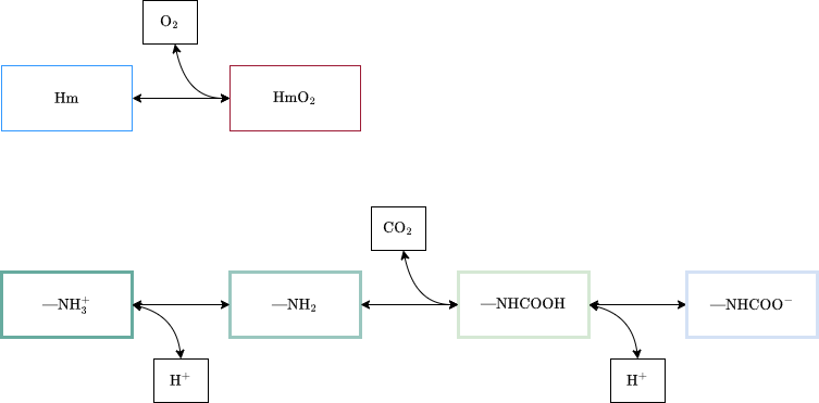
Figure 1: Reversible binding/unbinding reactions that occur in our model on each of the four subunits of hemoglobin. Top row: binding/unbinding of $\text{O}_{2}$, with “Hm” denoting the heme. Bottom row: binding/unbinding of $\text{H}^{+}$ and $\text{CO}_{2}$, with “N” denoting the N-terminal nitrogen and with “—” denoting the rest of the polypeptide chain.

In the top row of Figure 1, Hm refers to the heme which can which can bind the oxygen molecule; in the bottom row, N is the N-terminal nitrogen of the animo acid chain, and — refers to the rest of the chain. We assume for now that the top-row reactions of Figure 1 occur independently of the bottom-row reactions even when they occur on the same subunit, and also that any reactions occurring on different subunits occur independently of each other. These are provisional assumptions that will be modified later. To be specific, independence will be replaced by conditional independence, see below. By the law of mass action, we have the following equilibrium constants:

$$K_{\text{O}_{2}} =\dfrac{[\text{O}_{2}]\mathbb{P}(\text{Hm})}{\mathbb{P}({\text{HmO}_{2}})}$$ (1)

$$K_{\text{H}^{+},1} =\dfrac{[\text{H}^{+}]\mathbb{P}(\text{---NH}_{2})}{\mathbb{P}(\text{---NH}_{3}^{+})}$$ (2)

$$K_{\text{CO}_{2}} =\dfrac{[\text{CO}_{2}]\mathbb{P}(\text{---NH}_{2})}{\mathbb{P}(\text{---NHCOOH})}$$ (3)

$$K_{\text{H}^{+},2} =\dfrac{[\text{H}^{+}]\mathbb{P}(\text{---NHCOO}^{-})}{\mathbb{P}(\text{---NHCOOH})}$$ (4)

Here $[\,\cdot\,]$ denotes equilibrium molar concentration of $\text{O}_{2},\text{CO}_{2},\text{or H}^{+}$, and $\mathbb{P}(\,\cdot\,)$ denotes the equilibrium probability that the subunit is in the given state. Note that this way of writing equilibrium constants is equivalent to the standard way, since the equilibrium probability can be written as the equilibrium molar concentration of the given state divided by the sum of equilibrium molar concentrations of all possible states, and when this is applied to (1-4), we recover the standard formulae.

For the heme, we have the following two equations:

$$K_{\text{O}_{2}}\mathbb{P}({\text{HmO}_{2}})=[\text{O}_{2}]\mathbb{P}(\text{Hm})$$ (5)

$$\mathbb{P}({\text{HmO}_{2}})+\mathbb{P}(\text{Hm})=1$$ (6)

and it follows that

$$\mathbb{P}(\text{Hm})=\dfrac{K_{\text{O}_{2}}}{K_{\text{O}_{2}}+[\text{O}_{2}]},\ \ \mathbb{P}({\text{HmO}_{2}})=\dfrac{[\text{O}_{2}]}{K_{\text{O}_{2}}+[\text{O}_{2}]}$$ (7)

For the N-terminal group, we have the three equations (2-4) together with

$$\mathbb{P}(\text{---NH}_{3}^{+})+\mathbb{P}(\text{---NH}_{2})+\mathbb{P}(\text{---NHCOO}^{-})+\mathbb{P}(\text{---NHCOOH})=1$$ (8)

By using (2-4) to eliminate eliminate all variables other than $\mathbb{P}(\text{---NH}_{3}^{+})$, we can obtain

$$\mathbb{P}(\text{---NH}_{3}^{+})\left(1+\dfrac{K_{\text{H}^{+},1}}{[\text{H}^{+}]}\left(1+\dfrac{[\text{CO}_{2}]}{K_{\text{CO}_{2}}}\left(1+\dfrac{K_{\text{H}^{+},2}}{[\text{H}^{+}]}\right)\right)\right)=1$$ (9)

and therefore

$$\mathbb{P}(\text{---NH}_{3}^{+})=\dfrac{1}{1+\dfrac{K_{\text{H}^{+},1}}{[\text{H}^{+}]}\left(1+\dfrac{[\text{CO}_{2}]}{K_{\text{CO}_{2}}}\left(1+\dfrac{K_{\text{H}^{+},2}}{[\text{H}^{+}]}\right)\right)}$$ (10)

If needed, all probabilities of the other states can then be found from (2-4).

2.2 Allosteric Formulation

Now we introduce the allosteric model (Monod et al. 1965), which assumes that the hemoglobin molecule, as a whole, can exist in either of two global states denoted T(tense) and R(relaxed), and that the equilibrium constants defined above may depend on which global state the molecule is in. Thus, instead of equations (1-4), we have:

$$K_{\text{O}_{2}}^{G} =\dfrac{[\text{O}_{2}]\mathbb{P}(\text{Hm}|G)}{\mathbb{P}({\text{HmO}_{2}}|G)}$$ (11)

$$K_{\text{H}^{+},1}^{G} =\dfrac{[\text{H}^{+}]\mathbb{P}(\text{---NH}_{2}|G)}{\mathbb{P}(\text{---NH}_{3}^{+}|G)}$$ (12)

$$K_{\text{CO}_{2}}^{G} =\dfrac{[\text{CO}_{2}]\mathbb{P}(\text{---NH}_{2}|G)}{\mathbb{P}(\text{---NHCOOH}|G)}$$ (13)

$$K_{\text{H}^{+},2}^{G} =\dfrac{[\text{H}^{+}]\mathbb{P}(\text{---NHCOO}^{-}|G)}{\mathbb{P}(\text{---NHCOOH}|G)}$$ (14)

Here $\mathit{G}$ denotes the global state of hemoglobin molecule, $\mathit{G}$ = T or R, and $\mathbb{P}(\,\cdot\,|G)$ denotes conditional probability given the global state. The central assumption of the allosteric model can now be stated: that reactions occurring on different subunits are conditionally independent, the condition being the global state $\mathit{G}$ = T or R. We further assume that this conditional independence holds as well for the reactions depicted in the two rows of Figure 1, even when those reactions occur on the same subunit of hemoglobin.

To characterize the equilibrium between the two global states T and R in order to complete the model, it is sufficient to consider the special case in which the reaction between the T and R states occurs with no $\text{O}_{2}$ molecules bound and with all four N-terminal groups in the state $\text{---NH}_{3}^{+}$. The sufficiency of considering only one special case of the T $\leftrightarrow$ R equilibrium is a consequence of the principle of detailed balance, see Appendix A.

Accordingly, we define

$$L=\dfrac{\mathbb{P}(\text{Hm}|\text{R})^{4}\mathbb{P}(\text{---NH}_{3}^{+}|\text{R})^{4}\mathbb{P}(\text{R})}{\mathbb{P}(\text{Hm}|\text{T})^{4}\mathbb{P}(\text{---NH}_{3}^{+}|\text{T})^{4}\mathbb{P}(\text{T})}$$ (15)

so that $L$ is the equilibrium constant for the reaction $(\text{Hm}_{4}$—$(\text{NH}_{3}^{+})_{4})^{\text{T}}\leftrightarrow(\text{Hm}_{4}$—$(\text{NH}_{3}^{+})_{4})^{\text{R}}$. Note the use of conditional independence in the numerator and in the denominator of the formula for $L$. Here $\mathbb{P}(\text{R})$ and $\mathbb{P}(\text{T})$ denote the probability of the global states R and T respectively. These probabilities satisfy:

$$\mathbb{P}(\text{R})+\mathbb{P}(\text{T})=1$$ (16)

and we can solve (15-16) for $\mathbb{P}(\text{R})$ and $\mathbb{P}(\text{T})$ with following results

$$\mathbb{P}(\text{T})=\dfrac{\mathbb{P}(\text{Hm}|\text{R})^{4}\mathbb{P}(\text{---NH}_{3}^{+}|\text{R})^{4}}{L\mathbb{P}(\text{Hm}|\text{T})^{4}\mathbb{P}(\text{---NH}_{3}^{+}|\text{T})^{4}+\mathbb{P}(\text{Hm}|\text{R})^{4}\mathbb{P}(\text{---NH}_{3}^{+}|\text{R})^{4}}$$ (17)

$$\mathbb{P}(\text{R})=\dfrac{L\mathbb{P}(\text{Hm}|\text{T})^{4}\mathbb{P}(\text{---NH}_{3}^{+}|\text{T})^{4}}{L\mathbb{P}(\text{Hm}|\text{T})^{4}\mathbb{P}(\text{---NH}_{3}^{+}|\text{T})^{4}+\mathbb{P}(\text{Hm}|\text{R})^{4}\mathbb{P}(\text{---NH}_{3}^{+}|\text{R})^{4}}$$ (18)

In the above equations

$$\mathbb{P}(\text{Hm}|G)=\dfrac{1}{1+\dfrac{[\text{O}_{2}]}{K_{\text{O}_{2}}^{G}}}$$ (19)

and

$$\mathbb{P}(\text{---NH}_{3}^{+}|G) =\dfrac{1}{1+\dfrac{K_{\text{H}^{+},1}^{G}}{[\text{H}^{+}]}\left(1+\dfrac{[\text{CO}_{2}]}{K_{\text{CO}_{2}}^{G}}\left(1+\dfrac{K_{\text{H}^{+},2}^{G}}{[\text{H}^{+}]}\right)\right)}$$ (20)

where $G$ = T or R, from (7) and (10 - 14).

With $\mathbb{P}(\text{R})$ and $\mathbb{P}(\text{T})$ known, it is straightforward to evaluate the saturation of hemoglobin by oxygen, denoted $S_{\text{O}_{2}}$, which is the probability that any particular heme has $\text{O}_{2}$ bound to it, as follows

$$S_{\text{O}_{2}}=\mathbb{P}(\text{HmO}_{2})=\mathbb{P}(\text{HmO}_{2}|\text{T})\mathbb{P}(\text{T})+\mathbb{P}(\text{HmO}_{2}|\text{R})\mathbb{P}(\text{R})$$ (21)

where

$$\mathbb{P}(\text{HmO}_{2}|G)=\dfrac{[\text{O}_{2}]}{[\text{O}_{2}]+K_{\text{O}_{2}}^{G}}$$ (22)

for $G$ = T or R, see equation (7).

In (17 - 18) for $\mathbb{P}(\text{R})$ and $\mathbb{P}(\text{T})$, we can divide numerator and denominator by $\mathbb{P}(\text{---NH}_{3}^{+}|\text{R})^{4}$, and this gives the simpler results:

$$\mathbb{P}(\text{T})=\dfrac{\mathbb{P}(\text{Hm}|\text{R})^{4}}{\widetilde{L}\mathbb{P}(\text{Hm}|\text{T})^{4}+\mathbb{P}(\text{Hm}|\text{R})^{4}}$$ (23)

$$\mathbb{P}(\text{R})=\dfrac{\widetilde{L}\mathbb{P}(\text{Hm}|\text{T})^{4}}{\widetilde{L}\mathbb{P}(\text{Hm}|\text{T})^{4}+\mathbb{P}(\text{Hm}|\text{R})^{4}}$$ (24)

where

$$\widetilde{L}=L\dfrac{\mathbb{P}(\text{---NH}_{3}^{+}|\text{T})^{4}}{\mathbb{P}(\text{---NH}_{3}^{+}|\text{R})^{4}}$$ (25)

Note that although $L$ is constant, $\widetilde{L}$ is a function of $[\text{CO}_{2}]$ and $[\text{H}^{+}]$, see equation (20) with $\mathit{G}$ = T or R. Also note that $\widetilde{L}$ is independent of $[\text{O}_{2}]$. This is a special case of a general property of the allosteric model (Monod et al. 1965) that allosteric modulators have their effect via modification of the equilibrium constant of the transition between the two global states T and R.

By substituting (15) into (25), we see that

$$\widetilde{L}=\dfrac{\mathbb{P}(\text{Hm}|\text{R})^{4}\mathbb{P}(\text{R})}{\mathbb{P}(\text{Hm}|\text{T})^{4}\mathbb{P}(\text{T})}$$ (26)

This is the effective equilibrium constant for the transition R and T in a hemoglobin molecule with no oxygen molecules bound. This equilibrium ”constant” is a function, however, of $[\text{CO}_{2}]$ and $[\text{H}^{+}]$.

What the foregoing shows is that when $[\text{CO}_{2}]$ and $[\text{H}^{+}]$ are held constant, our model takes the form of an allosteric model for $\text{O}_{2}$ binding only, and when $[\text{CO}_{2}]$ and $[\text{H}^{+}]$ are varied, the only change is a change in the effective equilibrium constant for the transition between T and R.

Substitution of (23 - 24) into (21) gives a more explicit formula for $S_{\text{O}_{2}}$:

$$S_{\text{O}_{2}} =\dfrac{\mathbb{P}(\text{HmO}_{2}|\text{T})\mathbb{P}(\text{Hm}|\text{R})^{4}+\mathbb{P}(\text{HmO}_{2}|\text{R})\widetilde{L}\mathbb{P}(\text{Hm}|\text{T})^{4}}{\widetilde{L}\mathbb{P}(\text{Hm}|\text{T})^{4}+\mathbb{P}(\text{Hm}|\text{R})^{4}}$$

$$=\dfrac{\dfrac{1}{\widetilde{L}}\dfrac{\mathbb{P}(\text{HmO}_{2}|\text{T})}{\mathbb{P}(\text{Hm}|\text{T})^{4}}+\dfrac{\mathbb{P}(\text{HmO}_{2}|\text{R})}{\mathbb{P}(\text{Hm}|\text{R})^{4}}}{\dfrac{1}{\widetilde{L}}\dfrac{1}{\mathbb{P}(\text{Hm}|\text{T})^{4}}+\dfrac{1}{\mathbb{P}(\text{Hm}|\text{R})^{4}}}$$

$$=\dfrac{\dfrac{1}{\widetilde{L}}\left(1+\dfrac{[\text{O}_{2}]}{K_{\text{O}_{2}}^{\text{T}}}\right)^{3}\dfrac{[\text{O}_{2}]}{K_{\text{O}_{2}}^{\text{T}}}+\left(1+\dfrac{[\text{O}_{2}]}{K_{\text{O}_{2}}^{\text{R}}}\right)^{3}\dfrac{[\text{O}_{2}]}{K_{\text{O}_{2}}^{\text{R}}}}{\dfrac{1}{\widetilde{L}}\left(1+\dfrac{[\text{O}_{2}]}{K_{\text{O}_{2}}^{\text{T}}}\right)^{4}+\left(1+\dfrac{[\text{O}_{2}]}{K_{\text{O}_{2}}^{\text{R}}}\right)^{4}}$$ (27)

with $\widetilde{L}$ being the function of $[\text{CO}_{2}]$ and $[\text{H}^{+}]$ that is given by equation (25), with the right-hand side of (25) defined by the two instances of equation (20) obtained by setting $G$ = T or R:

$$\widetilde{L}=\left(\dfrac{1+\dfrac{K_{\text{H}^{+},1}^{\text{R}}}{[\text{H}^{+}]}\left(1+\dfrac{[\text{CO}_{2}]}{K_{\text{CO}_{2}}^{\text{R}}}\left(1+\dfrac{K_{\text{H}^{+},2}^{\text{R}}}{[\text{H}^{+}]}\right)\right)}{1+\dfrac{K_{\text{H}^{+},1}^{\text{T}}}{[\text{H}^{+}]}\left(1+\dfrac{[\text{CO}_{2}]}{K_{\text{CO}_{2}}^{\text{T}}}\left(1+\dfrac{K_{\text{H}^{+},2}^{\text{T}}}{[\text{H}^{+}]}\right)\right)}\right)^{4}L$$ (28)

3 Results

In this section we first do parameter fitting, and then we explore some consequences of the model with its parameters determined. Note that we do not make use of literature values of equilibrium constants, since equilibrium constants are model dependent, and previous authors have used different models from the one employed here.

In our model, the independent variables are the free concentrations of $\text{O}_{2}$, $\text{H}^{+}$, and $\text{CO}_{2}$. In the data that we use for parameter fitting, however, the experimentally controlled variables are the partial pressures in the cases of $\text{O}_{2}$ and $\text{CO}_{2}$, and the pH in the case of $\text{H}^{+}$. The conversions are given in Appendix B. In our figures showing comparisons to experimental data, we use the same variables as in the experimental literature, since these are more likely to be familiar to the reader.

3.1 Parameter fitting of the model with [$\text{H}^{+}$] and [$\text{CO}_{2}$] held constant

We first consider the case in which $[\text{CO}_{2}]$ and $[\text{H}^{+}]$ are held constant under the standard physiological conditions $[\text{H}^{+}]_{\text{std}}$ and $[\text{CO}_{2}]_{\text{std}}$. In this case equation (27) becomes

$$S_{\text{O}_{2}}=\dfrac{\dfrac{1}{L^{*}}\left(1+\dfrac{[\text{O}_{2}]}{K_{\text{O}_{2}}^{\text{T}}}\right)^{3}\dfrac{[\text{O}_{2}]}{K_{\text{O}_{2}}^{\text{T}}}+\left(1+\dfrac{[\text{O}_{2}]}{K_{\text{O}_{2}}^{\text{R}}}\right)^{3}\dfrac{[\text{O}_{2}]}{K_{\text{O}_{2}}^{\text{R}}}}{\dfrac{1}{L^{*}}\left(1+\dfrac{[\text{O}_{2}]}{K_{\text{O}_{2}}^{\text{T}}}\right)^{4}+\left(1+\dfrac{[\text{O}_{2}]}{K_{\text{O}_{2}}^{\text{R}}}\right)^{4}}$$ (29)

with $L^{*}$ as the following constant

$$L^{*}=\left(\dfrac{1+\dfrac{K_{\text{H}^{+},1}^{\text{R}}}{[\text{H}^{+}]_{\text{std}}}\left(1+\dfrac{[\text{CO}_{2}]_{\text{std}}}{K_{\text{CO}_{2}}^{\text{R}}}\left(1+\dfrac{K_{\text{H}^{+},2}^{\text{R}}}{[\text{H}^{+}]_{\text{std}}}\right)\right)}{1+\dfrac{K_{\text{H}^{+},1}^{\text{T}}}{[\text{H}^{+}]_{\text{std}}}\left(1+\dfrac{[\text{CO}_{2}]_{\text{std}}}{K_{\text{CO}_{2}}^{\text{T}}}\left(1+\dfrac{K_{\text{H}^{+},2}^{\text{T}}}{[\text{H}^{+}]_{\text{std}}}\right)\right)}\right)^{4}L$$ (30)

Note that $L^{*}$ is the value of $\widetilde{L}$ that is obtained by substituting (20) into (25) in the special case that $[\text{H}^{+}]=[\text{H}^{+}]_{\text{std}}=5.7544\times 10^{-8}\text{ moles/liter and }[\text{CO}_{2}]=[\text{CO}_{2}]_{\text{std}}=1.308\times 10^{-3}$ moles/liter. These values correspond to ($\text{pH})_{\text{std}}$ = 7.24 and ($\text{P}_{\text{CO}_{2}})_{\text{std}}$ = 40, see Appendix B.

To determine the equilibrium constants $K_{\text{O}_{2}}^{\text{R}}$, $K_{\text{O}_{2}}^{\text{T}}$ and $L^{*}$, we employ a least square fitting method with Matlab lsqcurvefit function using experimental data derived from Winslow et al. (1976). The best-fit calculated values are stated in Table 1:

Table 1: Best-fit values of the equilibrium constants that appear in Equation (29)

Symbol	Value	Unit
$K_{\text{O}_{2}}^{\text{R}}$	$2.1915\times 10^{-7}$	moles/liter
$K_{\text{O}_{2}}^{\text{T}}$	$1.1284\times 10^{-5}$	moles/liter
$L^{*}$	$2.6513\times 10^{3}$	—

Figure 2 shows the fitted result with parameters stated in Table 1, together with the experimental data from which those parameters were derived. A measure of the quality of the fit is the $\text{R}^{2}$ value, which is 0.9979.

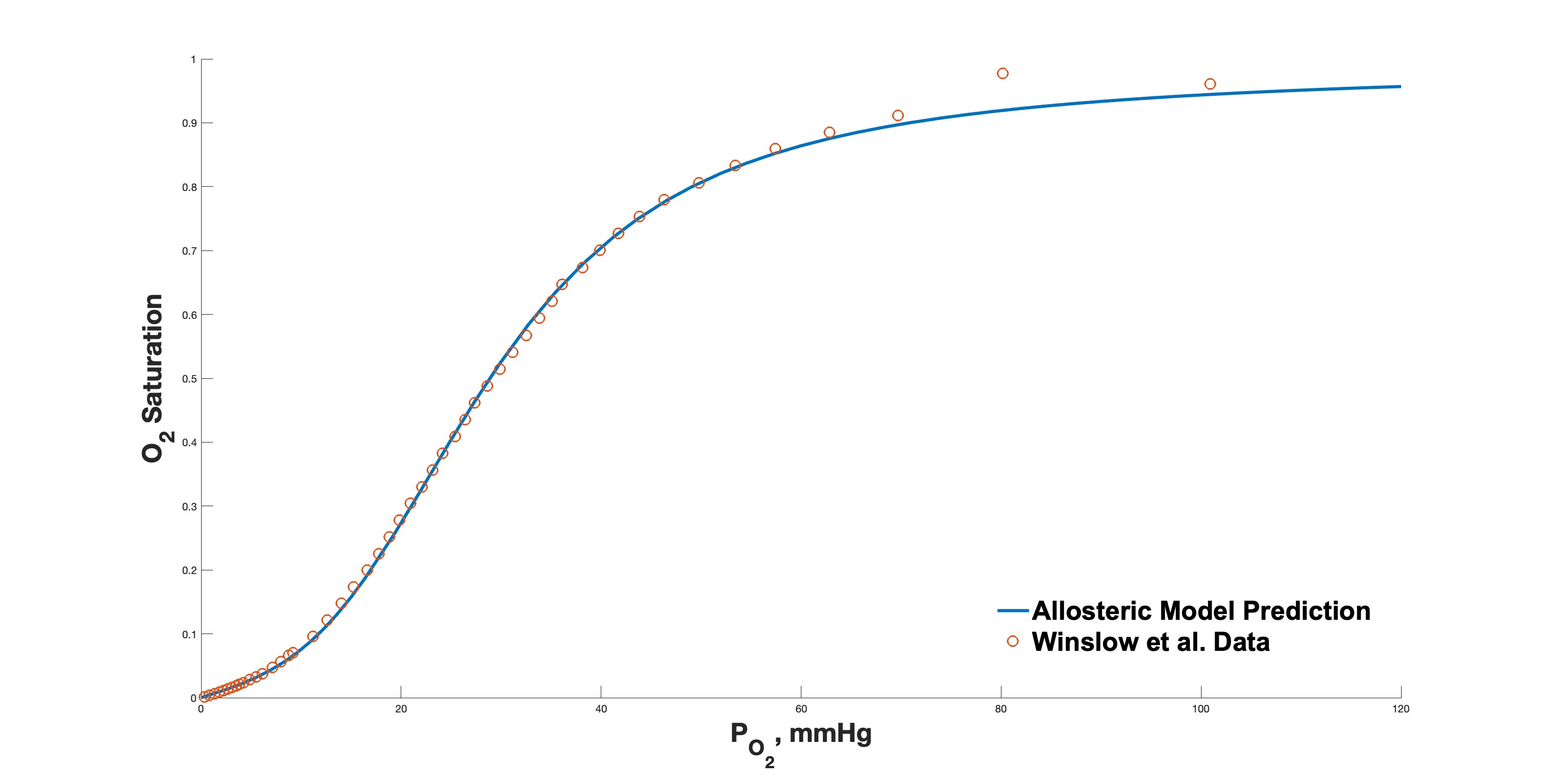
Figure 2: Oxygen saturation ($\text{S}_{\text{O}_{2}}$) as a function of the partial pressure of oxygen ($\text{P}_{\text{O}_{2}}$), with $\text{P}_{\text{CO}_{2}}$ and pH held constant. Solid curve is a plot of equation (29) with parameters shown in Table 1, but note that [$\text{O}_{2}$] has here been plotted in terms of $\text{P}_{\text{O}_{2}}$, see Appendix B. Circles plot the experimental data from Winslow et al. (1976) that were used to determine the parameters. Coefficient of determination is $\text{R}^{2}$ = 0.9979.

3.2 Determination of the parameters that govern the interactions of $\text{H}^{+}$ and $\text{CO}_{2}$ with the N-terminal group of hemoglobin

The purpose of this section is to determine the values of all of the remaining parameters, namely the six equilibrium constants associated with reactions at the N-terminal group (three for each of the states T and R), and also the parameter $L$ that is the equilibrium constant of the T $\leftrightarrow$ R transition (in a particular state, with all four N-terminal groups in the form —$\text{NH}_{3}^{+}$, and with all four hemes having no oxygen bound). We assume here that the values of $K_{\text{O}_{2}}^{\text{T}}$, $K_{\text{O}_{2}}^{\text{R}}$, and $L^{*}$ are already known, since they have been determined in the previous section and therefore have the values that are stated in Table 1.

With $L^{*}$ regarded as known, the parameter $L$ becomes an explicit function of the 6 unknown equilibrium constants that we seek to determine here. This function is

$$L=\frac{L^{*}}{c}$$ (31)

where

$$c=\left(\dfrac{1+\dfrac{K_{\text{H}^{+},1}^{\text{R}}}{[\text{H}^{+}]_{\text{std}}}\left(1+\dfrac{[\text{CO}_{2}]_{\text{std}}}{K_{\text{CO}_{2}}^{\text{R}}}\left(1+\dfrac{K_{\text{H}^{+},2}^{\text{R}}}{[\text{H}^{+}]_{\text{std}}}\right)\right)}{1+\dfrac{K_{\text{H}^{+},1}^{\text{T}}}{[\text{H}^{+}]_{\text{std}}}\left(1+\dfrac{[\text{CO}_{2}]_{\text{std}}}{K_{\text{CO}_{2}}^{\text{T}}}\left(1+\dfrac{K_{\text{H}^{+},2}^{\text{T}}}{[\text{H}^{+}]_{\text{std}}}\right)\right)}\right)^{4}$$

This formula for $L$ follows from the definition of $L^{*}$ as the value of $\widetilde{L}$ when the concentrations of $\text{H}^{+}$ and $\text{CO}_{2}$ are at their standard values. By making use of the equation $L$ = $L^{*}/c$ with the value of $L^{*}$ known, we incorporate the previous determination of $L^{*}$ into the parameter fitting of the present section, and in this way we reduce the number of unknown parameters from seven to six.

We then apply the same least square fitting method with Matlab lsqcurvefit function to equation (27) and utilize experimental data on oxygen hemoglobin saturation from Joels and Pugh (1958), Kilmartin and Rossi-Bernardi (1973) and Woyke et al. (2022) to obtain the values summarized in Table 2.

Table 2: Best-fit values of the rest of the equilibrium constants that appear in Equation (27)

Symbol	Value	Unit
$L$	$3.1140\times 10^{-4}$	—
$K_{\text{H}^{+},1}^{\text{R}}$	$6.6279\times 10^{-4}$	moles/liter
$K_{\text{CO}_{2}}^{\text{R}}$	$0.4050$	moles/liter
$K_{\text{H}^{+},2}^{\text{R}}$	$7.5550\times 10^{-6}$	moles/liter
$K_{\text{H}^{+},1}^{\text{T}}$	$7.2101\times 10^{-8}$	moles/liter
$K_{\text{CO}_{2}}^{\text{T}}$	$8.3066\times 10^{-4}$	moles/liter
$K_{\text{H}^{+},2}^{\text{T}}$	$1.5880\times 10^{-8}$	moles/liter

Figure 3 shows the fitted result with parameters stated in Table 2 of our least square fitting analysis, incorporating $\text{CO}_{2}$ and $\text{H}^{+}$ as independent variables, compared with the experimental data obtained from Joels and Pugh (1958). The original dataset comprises three experimental groups distinguished by $\text{P}_{\text{CO}_{2}}$ of 15, 40, and 70 mmHg, and corresponding pH values of 7.5, 7.25, and 7.15, respectively. The experimental data points from Joels and Pugh (1958) are represented by color-matched circles. The fit is excellent at the highest $\text{P}_{\text{CO}_{2}}$ and lowest pH. It is still very good in the intermediate case, and not as good at the lowest $\text{P}_{\text{CO}_{2}}$ and highest pH. The $\text{R}^{2}$ values are shown in Table 3.

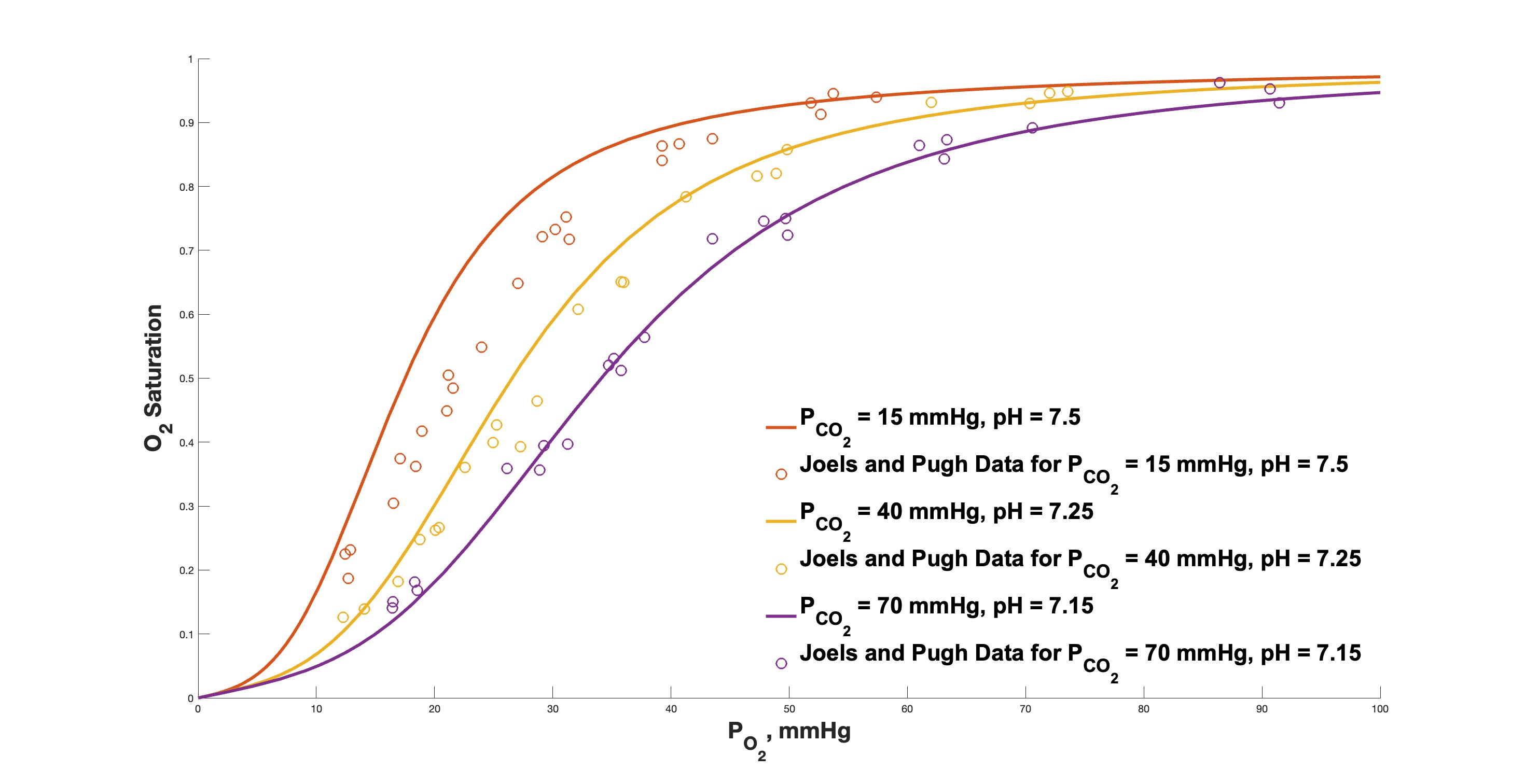
Figure 3: Oxygen saturation ($\text{S}_{\text{O}_{2}}$) as a function of the partial pressure of oxygen ($\text{P}_{\text{O}_{2}}$), with $\text{P}_{\text{CO}_{2}}$ with $\text{P}_{\text{CO}_{2}}$ and pH held constant in each of three cases: $\text{P}_{\text{CO}_{2}}$ = 15 mmHg, pH = 7.5; $\text{P}_{\text{CO}_{2}}$ = 40 mmHg, pH = 7.25; and $\text{P}_{\text{CO}_{2}}$ = 70 mmHg, pH = 7.15. Solid curve is a plot of equation (27) with parameters shown in Table 1 and Table 2. Circles plot the experimental data from Joels and Pugh (1958) that were used to determine the parameters in Table 2. Coefficients of determination are shown in Table 3, but note that these were not the only data used for that purpose, see also Figures 4 and 5.

Table 3: $\text{R}^{2}$ values of the allosteric model predictions on three sets of physiological conditions under data from Joels and Pugh (1958).

$\text{P}_{\text{CO}_{2}}(\text{mmHg})$	pH	$\text{R}^{2}$
15	7.5	0.82944
40	7.25	0.97423
70	7.15	0.99251

3.3 Oxygen $\text{P}_{50}$ as a function of pH and $\text{P}_{\text{CO}_{2}}$

Oxygen $\text{P}_{50}$ is the partial pressure of oxygen at which hemoglobin is 50 percent saturated, i.e., at which $\text{S}_{\text{O}_{2}}$ = 1/2. The value of the oxygen P50 is a function of pH and also of $\text{P}_{\text{CO}_{2}}$, and this relationship is often used as a way to assess the influence of pH and $\text{P}_{\text{CO}_{2}}$ on oxygen-hemoglobin binding.

In the present model, the oxygen $\text{P}_{50}$ is determined by

$$\dfrac{\dfrac{1}{\widetilde{L}}\left(1+\dfrac{[\text{O}_{2}]_{50}}{K_{\text{O}_{2}}^{\text{T}}}\right)^{3}\dfrac{[\text{O}_{2}]_{50}}{K_{\text{O}_{2}}^{\text{T}}}+\left(1+\dfrac{[\text{O}_{2}]_{50}}{K_{\text{O}_{2}}^{\text{R}}}\right)^{3}\dfrac{[\text{O}_{2}]_{50}}{K_{\text{O}_{2}}^{\text{R}}}}{\dfrac{1}{\widetilde{L}}\left(1+\dfrac{[\text{O}_{2}]_{50}}{K_{\text{O}_{2}}^{\text{T}}}\right)^{4}+\left(1+\dfrac{[\text{O}_{2}]_{50}}{K_{\text{O}_{2}}^{\text{R}}}\right)^{4}}=\dfrac{1}{2}$$ (32)

which we solve numerically for $[\text{O}_{2}]_{50}$ using the solve function in the Matlab symbolic toolbox, and then we convert $[\text{O}_{2}]_{50}$ to $\text{P}_{50}$ as described in Appendix B. In the above equation $K_{\text{O}_{2}}^{\text{T}}$ and $K_{\text{O}_{2}}^{\text{R}}$ have the values stated in Table 1. The parameter $\widetilde{L}$ is not constant, but instead is the function of [$\text{H}^{+}$] and [$\text{CO}_{2}$] that is given by equation (28) with parameters as stated in in Table 2. Thus, to evaluate the oxygen $\text{P}_{50}$ for any particular pH and $\text{P}_{\text{CO}_{2}}$, we first convert the given pH to $[\text{H}^{+}]$ and the given $\text{P}_{\text{CO}_{2}}$ to $[\text{CO}_{2}]$ as in Appendix B, then we evaluate $\widetilde{L}$ as above, solve equation (32) for $[\text{O}_{2}]_{50}$, and finally convert $[\text{O}_{2}]_{50}$ to $\text{P}_{50}$ by using the conversion from $[\text{O}_{2}]$ to $\text{P}_{\text{O}_{2}}$ that is stated in Appendix B.

For comparison, we state two empirical formulae for the oxygen $\text{P}_{50}$ that have appeared in the literature:

$$\text{P}_{50}^{\text{DB}}=26.8-21.279(\text{pH}_{\text{rbc}}-7.24)+8.872(\text{pH}_{\text{rbc}}-7.24)^{2}$$

$$+0.0482(\text{P}_{\text{CO}_{2}}-40)+3.64\text{E}-5(\text{P}_{\text{CO}_{2}}-40)^{2}$$ (33)

$$\text{P}_{50}^{\text{K}}=26.8\times 10^{0.4(7.24-\text{pH}_{\text{rbc}})+0.06\log\left(\dfrac{\text{P}_{\text{CO}_{2}}}{40}\right)}$$ (34)

Equation (33) is from Dash and Bassingthwaighte (2010), see also Buerk and Bridges (1986). Equation (34) is from Kelman (1966). In both formulae, the units of partial pressure are mmHg. The ”log” in the Kelman formula is base 10.

In Figure 4 we plot the oxygen $\text{P}_{50}$ as a function of pH with $\text{P}_{\text{CO}_{2}}$ fixed, and in Figure 5 we plot the oxygen $\text{P}_{50}$ as a function of $\text{P}_{\text{CO}_{2}}$ with pH fixed. In both figures we show the three predictions (the prediction of our model, and those of the empirical formulae in equations (33) and (34)) of $\text{P}_{50}$ as solid curves, and the experimental data as open circles. The allosteric model of the present paper is the clear winner here: it comes substantially closer to the experimental data than either of the empirical formulae, but to be fair we should note that the allosteric model was tuned in part to these data (see previous section), and it is possible that the empirical formulae would do as well if similarly tuned. The $\text{R}^{2}$ values of the fits of our model predictions to the experimental data are 0.94714 and 0.94661 in Figures 4 and 5, respectively.

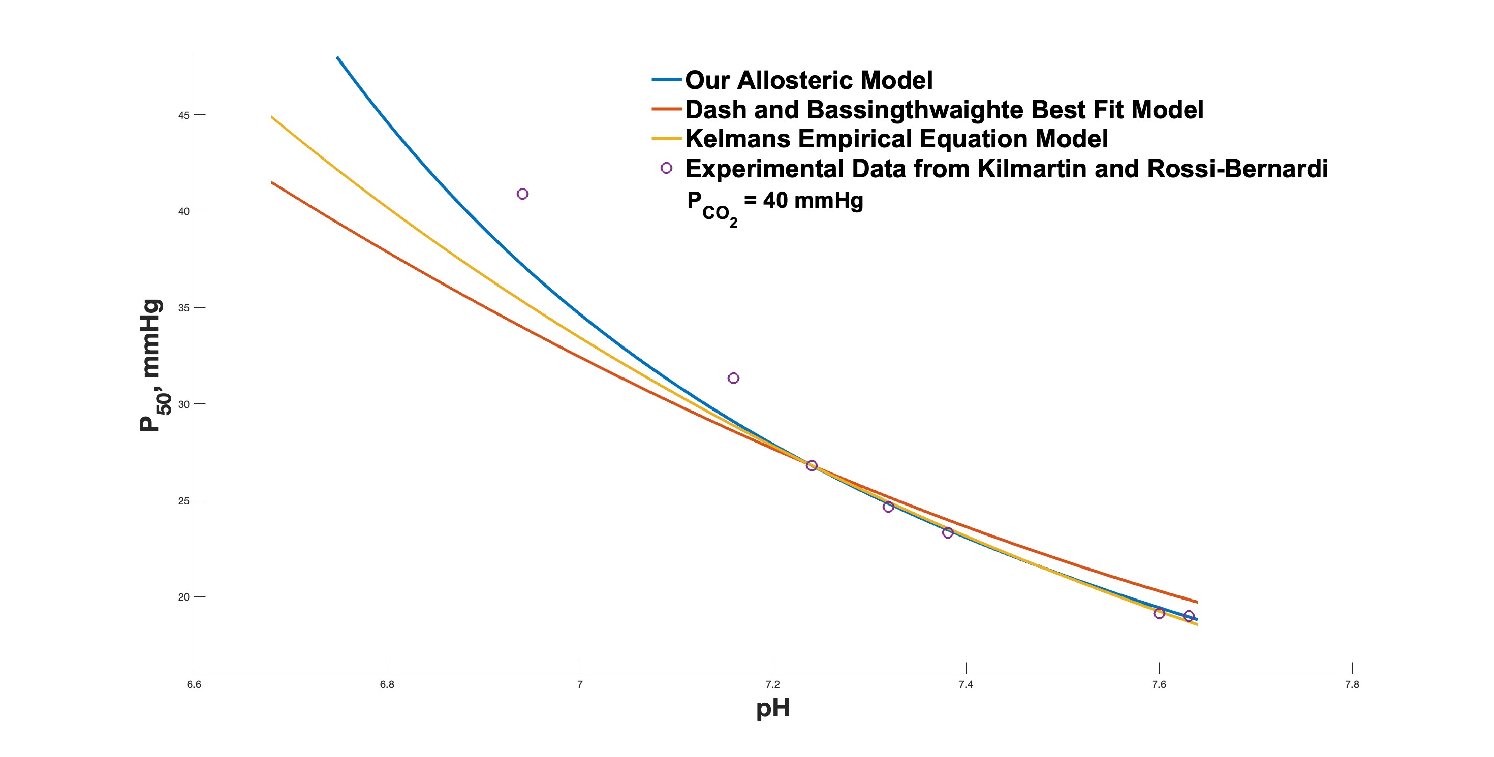
Figure 4: Oxygen $\text{P}_{50}$ as a function of pH with $\text{P}_{\text{CO}_{2}}$ = 40 mmHg. Model predictions are the solid lines, with blue for the present allosteric model, red for equation (33) from Dash and Bassingthwaighte (2010), and yellow for equation (34) from Kelman (1966). Purple circles are data points from Kilmartin and Rossi-Bernardi (1973).

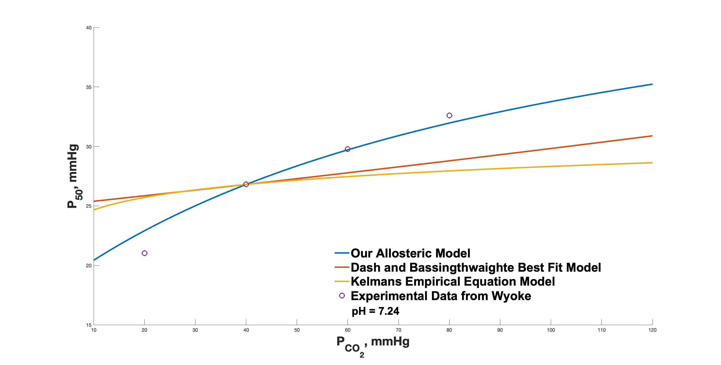
Figure 5: Oxygen $\text{P}_{50}$ as a function of $\text{P}_{\text{CO}_{2}}$ with pH = 7.24. Colors and symbols have the same meanings as in Figure 4, except that purple circles are data points from Woyke et al. (2022).

3.4 Components of the Bohr Effect

In order to study separately the allosteric influence exerted by [$\text{H}^{+}$] and [$\text{CO}_{2}$] on oxygen dissociation curves (ODCs), we fixed each one in turn of these allosteric effectors, setting it to its standard physiological level, and multiply the other by factors of 1/2, $1/\sqrt{2}$, 1, $\sqrt{2}$, 2 of its standard physiological level respectively. The resulting ODCs are shown in Figure 6 and Figure 7.

What is seen in these figures is a shift of the ODC curve to the right (i.e., decreased affinity for oxygen) with an increase in [$\text{H}^{+}$] (reduced pH) at fixed [$\text{CO}_{2}$], and likewise with an increase in [$\text{CO}_{2}$] at fixed [$\text{H}^{+}$]. These two effects are collectively known as the Bohr effect. The reason they have been considered as a single effect is that physiologically they go together, since $\text{CO}_{2}$ combines (catalyzed by carbonic anhydrase) with $\text{H}_{2}\text{O}$ to form $\text{H}_{2}\text{CO}_{3}$, which dissociates into $\text{H}\text{CO}_{3}^{-}$ and $\text{H}^{+}$. Here, however, we see the two components of the Bohr effect separately.

It is noteworthy that the shifts in the ODCs triggered by modifications in $\text{P}_{\text{CO}_{2}}$ are relatively subtle in contrast to those induced by changes in pH.

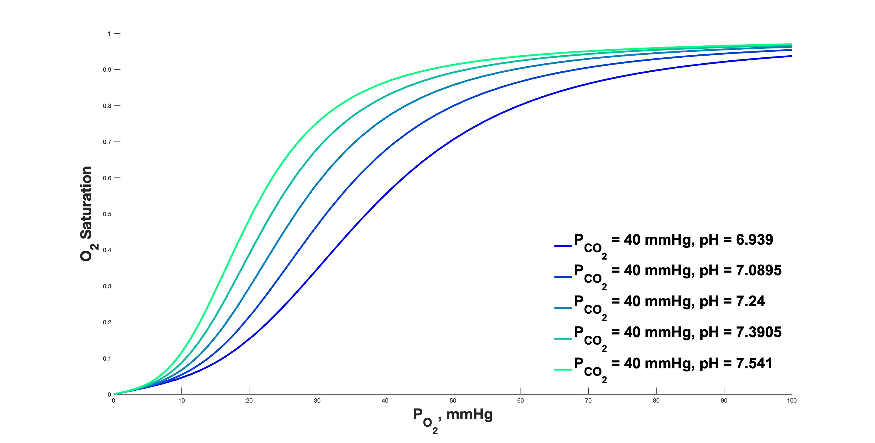
Figure 6: Oxygen saturation ($\text{S}_{\text{O}_{2}}$) as a function of the partial pressure of oxygen ($\text{P}_{\text{O}_{2}}$), with constant $\text{P}_{\text{CO}_{2}}$ = 40 mmHg and pH = 6.939, 7.0895, 7.24, 7.3905, and 7.541, as calculated from the equation provided in (27).

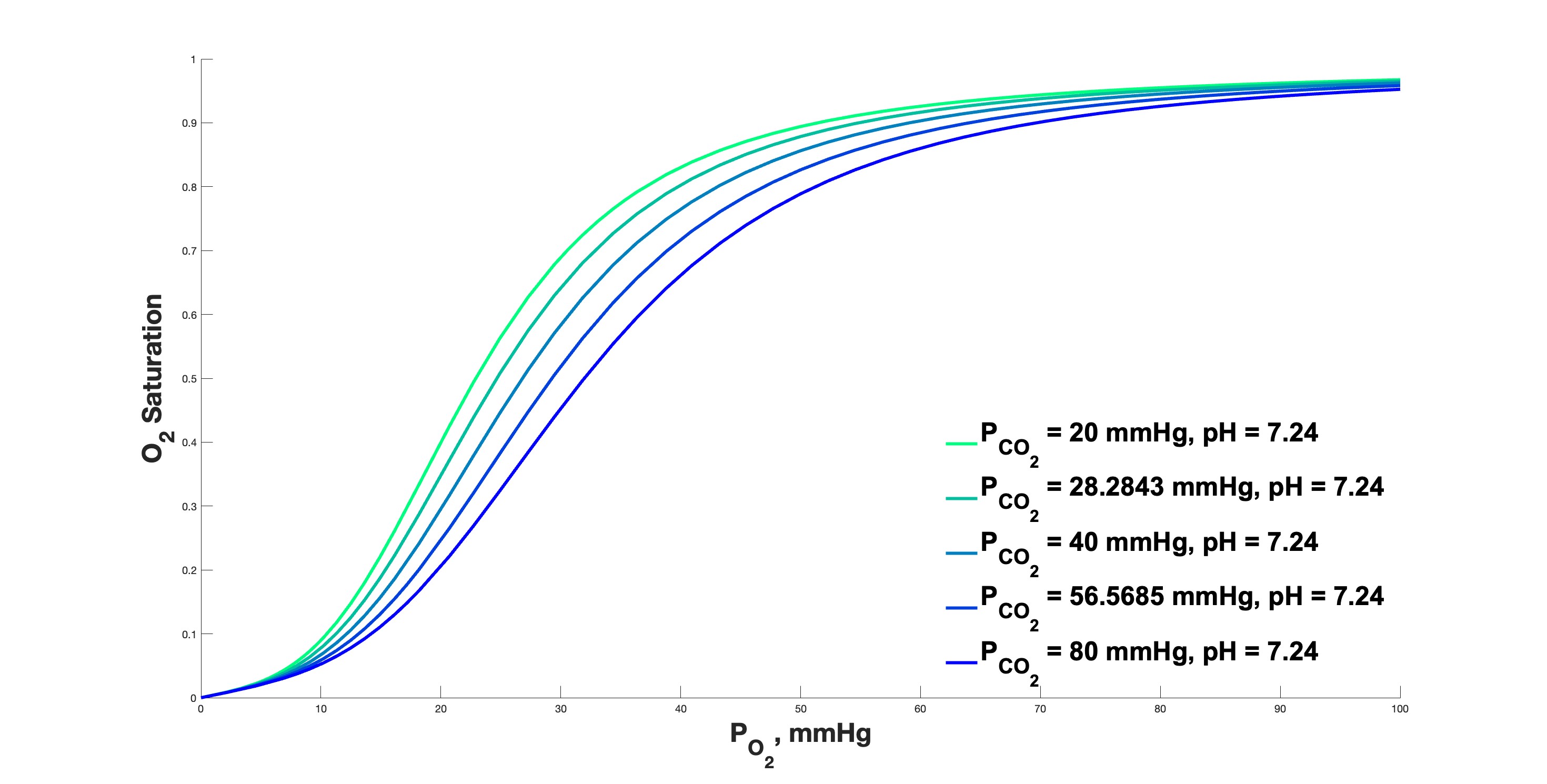
Figure 7: Oxygen saturation ($\text{S}_{\text{O}_{2}}$) as a function of the partial pressure of oxygen ($\text{P}_{\text{O}_{2}}$), with $\text{P}_{\text{CO}_{2}}$ = 20, 28.2842, 40, 56.685, 80 mmHg and constant pH = 7.24, as calculated from the equation provided in (27).

4 Sensitivity Analysis

We explore the local sensitivity of all model parameters, as delineated in Tables 1 and 2, employing a One-At-A-Time sensitivity measure, as outlined by Hamby (1994). This measure evaluates the percentage change in the residual sum of squares (RSS) between our model output and N experimental data points when each parameter is individually adjusted by $\pm$20%.

$$C(\theta_{i},\theta_{i}^{*})=\dfrac{|\sum_{j=1}^{N}(S_{\text{O}_{2}}(\theta_{i},x_{j})-y_{j})^{2}-\sum_{j=1}^{N}(S_{\text{O}_{2}}(\theta_{i}^{*},x_{j})-y_{j})^{2}|}{\sum_{j=1}^{N}(S_{\text{O}_{2}}(\theta_{i},x_{j})-y_{j})^{2}}$$ (35)

where $\theta_{i}\in\{L,K_{\text{O}_{2}}^{\text{R}},K_{\text{O}_{2}}^{\text{T}},K_{\text{H}^{+},1}^{\text{R}},K_{\text{CO}_{2}}^{\text{R}},K_{\text{H}^{+},2}^{\text{R}},K_{\text{H}^{+},1}^{\text{T}},K_{\text{CO}_{2}}^{\text{T}},K_{\text{H}^{+},2}^{\text{T}}\}$ is the parameter we are analysing, $\theta_{i}^{*}$ is the modified parameter, $x_{j}=([\text{O}_{2}]_{j},[\text{CO}_{2}]_{j},[\text{H}^{+}]_{j})$ is the jth inputting experiment data, and $y_{j}$ is the measured oxygen saturation corresponding to $x_{j}$. Therefore $S_{\text{O}_{2}}(\theta_{i}^{*},x_{j})$ denoted the model predicted saturation at given inputting level $x_{j}$ with all parameters at the level of Tables 1 and 2 except for $\theta_{i}$ adjusted to $\theta_{i}^{*}$.

After applying (35) to experimental data from Winslow et al. (1976), Joels and Pugh (1958), and Woyke et al.(2022), we obtain the following local sensitivity as shown in Table. 4. We saw that the percentage changes in RSS is bounded by the percentage perturbation we applied on the parameters, which demonstrates that the fit of our model to experimental data is not too sensitive to any one of the model’s parameters.

Table 4: Local sensitivities, $C(\theta_{i},\theta_{i}^{*})$, of model parameters to changes in their values. Each parameter, $\theta_{i}$, was adjusted up and down by 20% (yielding $\theta_{i}^{*}=0.8\theta_{i}$ and $\theta_{i}^{*}=1.2\theta_{i}$, respectively), and the resulting change in the Residual Sum of Squares (RSS) between the model output and experimental data was calculated using Eq. (35). The parameters originate from the equilibrium constants listed in Tables 1 and 2.

Parameter($\theta_{i}$)	$C(\theta_{i},\theta_{i}^{*})$	$C(\theta_{i},\theta_{i}^{*})$
	($\theta_{i}^{*}=0.8\theta_{i}$)	($\theta_{i}^{*}=1.2\theta_{i}$)
$L$	0.065	0.148
$K_{\text{O}_{2}}^{\text{R}}$	0.013	0.109
$K_{\text{O}_{2}}^{\text{T}}$	0.081	0.170
$K_{\text{H}^{+},1}^{\text{R}}$	8.906e-05	5.937e-05
$K_{\text{CO}_{2}}^{\text{R}}$	0.111	0.131
$K_{\text{H}^{+},2}^{\text{R}}$	0.182	0.066
$K_{\text{H}^{+},1}^{\text{T}}$	0.036	0.127
$K_{\text{CO}_{2}}^{\text{T}}$	0.110	0.081
$K_{\text{H}^{+},2}^{\text{T}}$	0.010	0.093

It is noteworthy that variations of $K_{\text{H}^{+},1}^{\text{R}}$ in both directions seem to exert a negligible impact on model performance. The parameter value found by our fitting procedure was almost $10^{-3}$ moles/liter (see Table 2). This means that in the R state of hemoglobin, we would have to get down to pH = 3 in order to see any significant amount of —$\text{NH}_{3}^{+}$ as the state of the N terminal. Since our data is far from that range of pH, all we can say from our fitting is that the N terminal state —$\text{NH}_{3}^{+}$ essentially does not happen when hemoglobin is in the R state. Thus our fitting procedure notices that $K_{\text{H}^{+},1}^{\text{R}}$ is large (in the above sense) but cannot determine how large. Note, however, that the corresponding parameter of the T state, $K_{\text{H}^{+},1}^{\text{R}}$ has a very different order of magnitude, and is indeed well-determined by our fitting procedure.

5 Summary and Conclusions

We have presented an allosteric model of the reversible binding of $\text{H}^{+}$, $\text{CO}_{2}$, and $\text{O}_{2}$ to hemoglobin. We have fit the model to experimental data, and thereby identified the model parameters. We have studied the sensitivity of the fit to data by varying each of the model parameters in turn.

Our focus in this paper has been the influence of $\text{H}^{+}$ and $\text{CO}_{2}$ on oxygen-hemoglobin binding. These two influences are collectively known as the Bohr effect, and we have separately studied these two components of the Bohr effect. Although we have not done so here, our model can also be used to study the Haldane effect, which is the influence of $\text{O}_{2}$ on $\text{CO}_{2}$ binding by hemoglobin. More generally, our model makes it possible to evaluate the mean numbers of $\text{H}^{+}$, $\text{CO}_{2}$, and $\text{O}_{2}$ that will be bound to one hemoglobin molecule, as functions of the free concentrations of those three molecular species. There is a need for a model that can do this in the simulation of gas exchange in the lungs, and of acid-base balance. In these related subjects, hemoglobin plays a pivotal role.

A didactic contribution of this paper is the use of probability in the formulation of the allosteric model. This brings out most clearly the role of conditional independence in the statement of the allosteric model, and it also leads to the straightforward evaluation of results, without the enumeration of all possible states. This becomes increasingly important as the complexity of the model grows, e.g., if one wanted to allow for more $\text{H}^{+}$ binding sites.

Possible limitations of the present model are (1) that there may be additional sites not considered here at which $\text{H}^{+}$ or $\text{CO}_{2}$ can bind to hemoglobin, and/or (2) that the interaction of $\text{H}^{+}$ and $\text{CO}_{2}$ binding with O2 binding may not be purely allosteric. There could, for example, be direct interactions within each subunit of hemoglobin between an $\text{H}^{+}$ binding site or a $\text{CO}_{2}$ binding site with the heme of that subunit. By insisting on only allosteric interaction, however, we avoid what would otherwise be a rapid proliferation of parameters.

Declarations

Competing interests

The authors declare that they have no known competing financial interests or personal relationships that could have appeared to influence the work reported in this paper.

Data availability

The datasets generated during and/or analysed during the current study are available from the author on reasonable request.

Appendix A Chemical-Kinetic Formulation of the Allosteric Model

A.1 Reactions Involving Oxygen Binding and Unbinding in the Heme

A.1.1 Reaction Scheme

The equilibrium reaction scheme of the allosteric model under standard physiological conditions is depicted in Figure 8. The two global states of hemoglobin are commonly referred to as the T(tense) state and the R(relaxed) state. The number of oxygen molecules bound to a hemoglobin molecule in a given state is indicated by a subscript, such that $\text{R}_{3}$ (for example) denotes a hemoglobin molecule in the R state with 3 oxygen molecules bound. Two equilibrium constants are introduced: $K_{\text{O}_{2}}^{\text{T}}$ and $K_{\text{O}_{2}}^{\text{R}}$, corresponding to the T and R states, respectively.

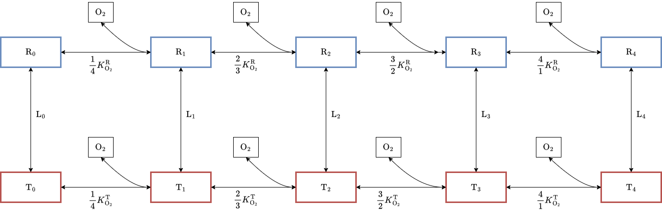
Figure 8: Reversible binding/unbinding of oxygen (horizontal reactions), and transitions (vertical reactions) between the two global states, T(tense) and R(relaxed), of hemoglobin. $K_{\text{O}_{2}}^{\text{R}}$ is the equilibrium constant for dissociation of O2 from any one of the heme groups when hemoglobin is in the R state, and $K_{\text{O}_{2}}^{\text{T}}$ has the same meaning but for hemoglobin in the T state. $L_{i}$ is the equilibrium constant for the R $\leftrightarrow$ T transition when there are $i$ molecules of $\text{O}_{2}$ bound to hemoglobin.

Note the numerical factors multiplying $K_{\text{O}_{2}}^{\text{R}}$ and $K_{\text{O}_{2}}^{\text{T}}$, which we shall explain in the context of the following reaction:

$$\ce{R_{i}+O_{2}<=>[\ce{(4-i)k_{\text{O}_{2}}^{R}}][\ce{(i+1)\gamma_{\text{O}_{2}}^{R}}]{\ce{R_{i+1}}}}$$ (36)

In this reaction, $k_{\text{O}_{2}}^{\text{R}}$ and $\gamma_{\text{O}_{2}}^{\text{R}}$ represent the forward and reverse rate constants, respectively. The forward rate constant is $(4-\text{i})k_{\text{O}_{2}}^{\text{R}}$, justified by the existence of $(4-i)$ unoccupied binding sites for oxygen, while the reverse rate constant is $(i+1)\gamma_{\text{O}_{2}}^{\text{R}}$, derived from the presence of $(i+1)$ bound oxygen molecules to $\text{R}_{i+1}$, available for dissociation.

At equilibrium, we have

$$\left(4-i\right)k_{\text{O}_{2}}^{\text{R}}[\text{R}_{i}][\text{O}_{2}]=\left(i+1\right)\gamma_{\text{O}_{2}}^{\text{R}}[\text{R}_{i+1}]$$ (37)

where the notation $[\,\cdot\,]$ denoted the concentration of given species. Solving the equation for the ratio of reactant concentrations yields

$$\dfrac{[\text{R}_{i}][\text{O}_{2}]}{[\text{R}_{i+1}]}=\dfrac{(i+1)\gamma_{\text{O}_{2}}^{\text{R}}}{(4-i)k_{\text{O}_{2}}^{\text{R}}}=\dfrac{i+1}{4-i}K_{\text{O}_{2}}^{\text{R}}$$ (38)

where $K_{\text{O}_{2}}^{\text{R}}=\dfrac{\gamma_{\text{O}_{2}}^{\text{R}}}{k_{\text{O}_{2}}^{\text{R}}}$ is the single-site equilibrium constant. Therefore, the dissociation equilibrium constant for reaction (36) can be expressed as $(\dfrac{i+1}{4-i})K_{\text{O}_{2}}^{\text{R}}$. Of course, the same reasoning is applicable to the T state, and that is why the numerical factors in the bottom row of Figure 8 are the same as those in the top row.

Note the implicit assumption in the foregoing that oxygen binding/unbinding at any one site is independent of the state of the other sites provided that we know the global state (T or R) of the hemoglobin molecule as a whole. This is the characteristic conditional independence assumption of the allosteric model.

A.1.2 Detailed Balance Analysis

The reaction scheme of Figure 8 seems to involve 7 equilibrium constants, $K_{\text{O}_{2}}^{\text{R}}$, $K_{\text{O}_{2}}^{\text{T}}$, and $L_{0}$ … $L_{4}$. Of these, however, only 3 are independent. To see this, note that the reaction scheme involves 4 loops, all four of which are of the form shown in Figure 9.

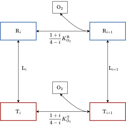
Figure 9: Generalized reversible binding/unbinding reactions that occur in our model on heme group of each hemoglobin molecule. Variables has the same meaning as Fig. 8.

According to the principle of detailed balance, within any loop in a reaction scheme, the product of the equilibrium constants must yield 1 (Alberty 2004). This principle, when applied to a counterclockwise circuit as seen in Figure 9, accounting for the direction of progression and definition of equilibrium constants, we can derive the following equation:

$$\left(\dfrac{i+1}{4-i}\right)K_{\text{O}_{2}}^{\text{R}}L_{i}\dfrac{1}{\left(\dfrac{i+1}{4-i}\right)K_{\text{O}_{2}}^{\text{T}}}\dfrac{1}{L_{i+1}}=1$$ (39)

Simplifying this yields:

$$\begin{cases}\begin{aligned} \dfrac{L_{i+1}}{L_{i}}&=\dfrac{K_{\text{O}_{2}}^{\text{R}}}{K_{\text{O}_{2}}^{\text{T}}}\\ \end{aligned}\\ \\ \begin{aligned} L_{i}=\left(\dfrac{K_{\text{O}_{2}}^{\text{R}}}{K_{\text{O}_{2}}^{\text{T}}}\right)^{i}L_{0}\end{aligned}\end{cases}$$ (40)

where $L_{i}$ is the equilibrium rate constant for the transition of $\text{R}_{i}$ to $\text{T}_{i}$. Consequently, $L_{i}$ forms a geometric sequence with a ratio of $\dfrac{K_{\text{O}_{2}}^{\text{R}}}{K_{\text{O}_{2}}^{\text{T}}}$. It is thus inferred that the entire allosteric scheme is characterized by three parameters: $K_{\text{O}_{2}}^{\text{R}}$, $K_{\text{O}_{2}}^{\text{T}}$, and $L_{0}$. Note that $K_{\text{O}_{2}}^{\text{R}}$ and $K_{\text{O}_{2}}^{\text{T}}$ have units of concentration, whereas $L_{0}$ is dimensionless.

A.1.3 Oxyhemoglobin Saturation

Equation (38) can be rewritten as follows:

$$\dfrac{[\text{R}_{i}]}{[\text{R}_{i-1}]}=\dfrac{4-i+1}{i}\dfrac{[\text{O}_{2}]}{K_{\text{O}_{2}}^{\text{R}}}$$ (41)

and this implies

$$\dfrac{[\text{R}_{i}]}{[\text{R}_{0}]}=\dfrac{(4)\ldots(4-i+1)}{1\ldots i}\left(\dfrac{[\text{O}_{2}]}{K_{\text{O}_{2}}^{\text{R}}}\right)^{i}=\dfrac{4!}{(4-i)!i!}\left(\dfrac{[\text{O}_{2}]}{K_{\text{O}_{2}}^{\text{R}}}\right)^{i}={4\choose i}\left(\dfrac{[\text{O}_{2}]}{K_{\text{O}_{2}}^{\text{R}}}\right)^{i}$$ (42)

Similarly

$$\dfrac{[\text{T}_{i}]}{[\text{T}_{0}]}={4\choose i}\left(\dfrac{[\text{O}_{2}]}{K_{\text{O}_{2}}^{\text{T}}}\right)^{i}$$ (43)

By definition of $L_{0}$, we also have

$$\dfrac{[\text{R}_{0}]}{[\text{T}_{0}]}=\dfrac{1}{L_{0}}$$ (44)

From (42-44), we can express the total concentration of hemoglobin, which we denote by $[\text{Hb}^{*}]$, and also the total concentration of bound oxygen, which we denote by $[\text{O}_{2}]_{\text{bound}}$, in terms of [$\text{T}_{0}$], which is the concentration of hemoglobin in the T state with no oxygen bound:

$$\begin{cases}\begin{aligned} &=\sum_{i=0}^{4}[\text{R}_{i}]+\sum_{i=0}^{4}[\text{T}_{i}]\\ &=[\text{T}_{0}]\left(\dfrac{1}{L_{0}}\sum_{i=0}^{4}{4\choose i}\left(\dfrac{[\text{O}_{2}]}{K_{\text{O}_{2}}^{\text{R}}}\right)^{i}+\sum_{i=0}^{4}{4\choose i}\left(\dfrac{[\text{O}_{2}]}{K_{\text{O}_{2}}^{\text{T}}}\right)^{i}\right)\end{aligned}\\ \\ \begin{aligned} {}_{\text{bound}}&=\sum_{i=0}^{4}i[\text{R}_{i}]+\sum_{i=0}^{4}i[\text{T}_{i}]\\ &=[\text{T}_{0}]\left(\dfrac{1}{L_{0}}\sum_{i=0}^{4}i{4\choose i}\left(\dfrac{[\text{O}_{2}]}{K_{\text{O}_{2}}^{\text{R}}}\right)^{i}+\sum_{i=0}^{4}i{4\choose i}\left(\dfrac{[\text{O}_{2}]}{K_{\text{O}_{2}}^{\text{T}}}\right)^{i}\right)\end{aligned}\end{cases}$$ (45)

To evaluate the sums in (45) we use the identities

$$\begin{cases}\begin{aligned} \sum_{k=0}^{n}{n\choose k}x^{k}=(1+x)^{n}\end{aligned}\\ \\ \begin{aligned} \sum_{k=1}^{n}k{n\choose k}x^{k}=nx(1+x)^{n-1}\end{aligned}\end{cases}$$

the first of which is the binomial theorem, and the second can be derived from the first by differentiation with respect to x followed by multiplication by x. Equation (45) then become:

$$\begin{cases}\begin{aligned} =[\text{T}_{0}]\left(\dfrac{1}{L_{0}}\left(1+\dfrac{[\text{O}_{2}]}{K_{\text{O}_{2}}^{\text{R}}}\right)^{4}+\left(1+\dfrac{[\text{O}_{2}]}{K_{\text{O}_{2}}^{\text{T}}}\right)^{4}\right)\end{aligned}\\ \\ \begin{aligned} {}_{\text{bound}}=4[\text{T}_{0}]\left(\dfrac{1}{L_{0}}\left(1+\dfrac{[\text{O}_{2}]}{K_{\text{O}_{2}}^{\text{R}}}\right)^{3}\dfrac{[\text{O}_{2}]}{K_{\text{O}_{2}}^{\text{R}}}+\left(1+\dfrac{[\text{O}_{2}]}{K_{\text{O}_{2}}^{\text{T}}}\right)^{3}\dfrac{[\text{O}_{2}]}{K_{\text{O}_{2}}^{\text{T}}}\right)\end{aligned}\end{cases}$$ (46)

and finally we can evaluate the saturation of hemoglobin as follows:

$$S_{\text{O}_{2}}=\dfrac{[\text{O}_{2}]_{\text{bound}}}{4[\text{Hb}^{*}]}=\dfrac{\dfrac{1}{L_{0}}\left(1+\dfrac{[\text{O}_{2}]}{K_{\text{O}_{2}}^{\text{R}}}\right)^{3}\dfrac{[\text{O}_{2}]}{K_{\text{O}_{2}}^{\text{R}}}+\left(1+\dfrac{[\text{O}_{2}]}{K_{\text{O}_{2}}^{\text{T}}}\right)^{3}\dfrac{[\text{O}_{2}]}{K_{\text{O}_{2}}^{\text{T}}}}{\dfrac{1}{L_{0}}\left(1+\dfrac{[\text{O}_{2}]}{K_{\text{O}_{2}}^{\text{R}}}\right)^{4}+\left(1+\dfrac{[\text{O}_{2}]}{K_{\text{O}_{2}}^{\text{T}}}\right)^{4}}$$ (47)

A.2 Reactions in Amino Group

A.2.1 General Reaction Schemes

The following section explores the reactions occurring within the N-terminal group of hemoglobin, and their effects on oxygen saturation. We specifically focus on three reactions that pertain to hemoglobin’s allosteric effectors:

$$\begin{cases}\begin{aligned} \text{Reaction}\ r_{1}:\ \ce{\text{---}NH3+&<=>H++\text{---}NH2}\end{aligned}\\ \\ \begin{aligned} \text{Reaction}\ r_{2}:\ \ce{\text{---}NH2+CO2&<=>\text{---}NHCOOH}\end{aligned}\\ \\ \begin{aligned} \text{Reaction}\ r_{3}:\ \ce{\text{---}NHCOOH&<=>\text{---}NHCOO^{-}+H+}\end{aligned}\end{cases}$$ (48)

As before, we use the notation R or T to denote which of the two global states a hemoglobin molecule is in, with a subscript $i$ = 0… 4 to denote the number of oxygen molecules bound. Superscripts $j,k,l,m$ (which will always appear in that order) indicate the numbers of the different occurrences in the hemoglobin molecule of each of the four possible states of the N-terminal amino groups. The superscript $j$ is the number of $\ce{\text{---}NH3+}$, $k$ is the number of $\ce{\text{---}NH2}$, $l$ is the number of $\ce{\text{---}NHCOOH}$, and $m$ is the number of $\ce{\text{---}NHCOO-}$. Thus, $j,k,l,m$ are non-negative integers such that $j+k+l+m$ = 4, since each of the four N-terminal amino groups has to be in one of those four states. For example $\text{T}_{2}^{2011}$ is a possible state of hemoglobin in which the global state is T, there are 2 oxygen molecules bound, 2 of the 4 N-terminal amino groups are in the state $\ce{\text{---}NH3+}$, there are no N-terminal amino groups in the state $\ce{\text{---}NH2}$, and there is one each of N-terminal amino groups in the states $\ce{\text{---}NHCOOH}$ and $\ce{\text{---}NHCOO-}$. Note that a key assumption of the allosteric model is that it does not matter which of the four subunits of hemoglobin are the ones that have oxygen bound, even when the subunits can be distinguished by different states of their N-terminal groups.

Figure 10 depicts all possible reactions involving the N-terminal groups for a hemoglobin molecule in the R state with $i$ oxygen molecules bound. Note, however, that the value of $i$ makes no difference, and also that the exact same diagram is applicable with R replaced by T.

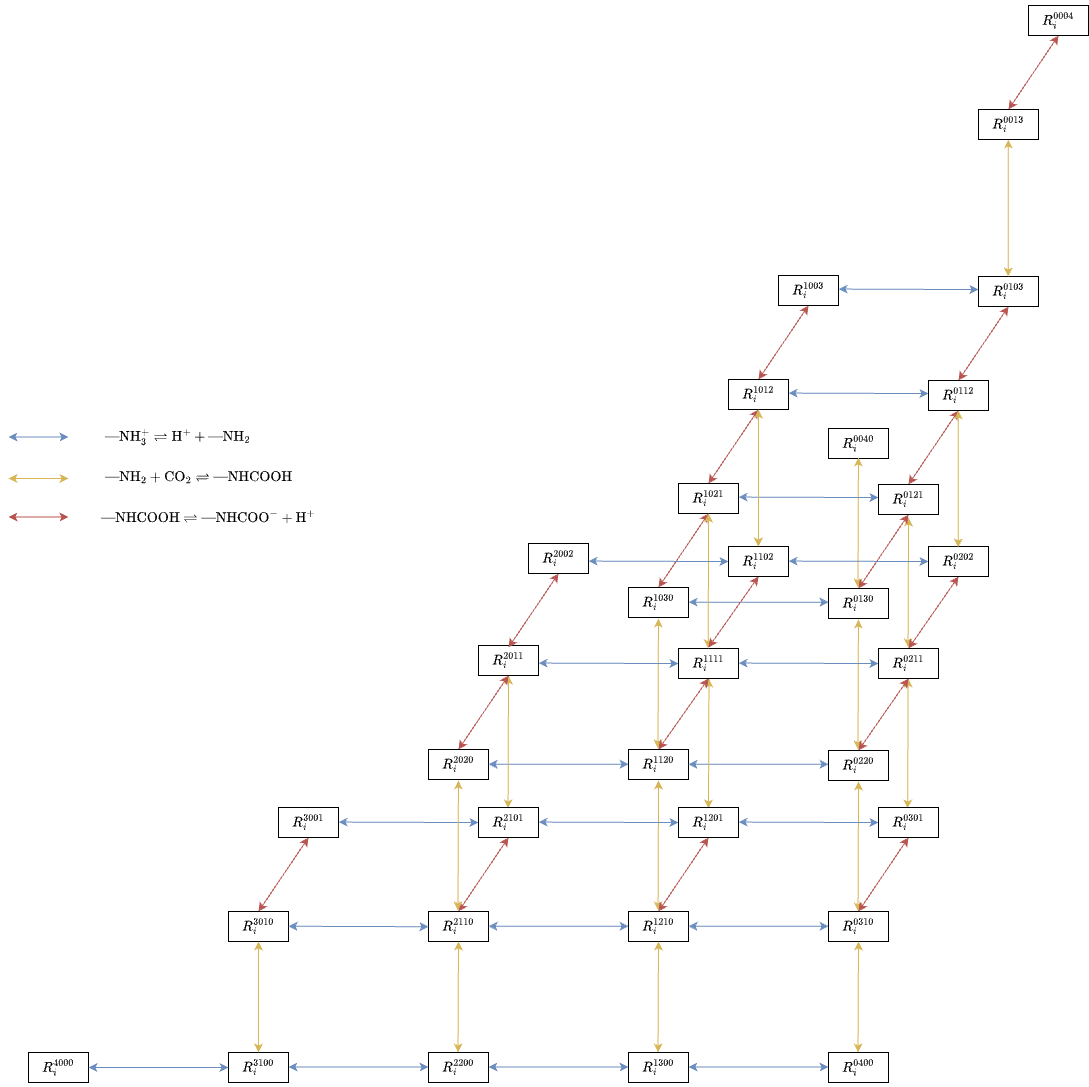
Figure 10: Reversible binding/unbinding reactions that occur in our model on N-terminal group of a R state hemoglobin molecule with $i$ bound oxygen molecules. “R” stands for the global state the hemoglobin, the subscript “$i$” describe the number of oxygen molecule bound to the hemoglobin molecule, and the superscript “$jklm$” denotes the number of subunit in the states of $\ce{\text{---}NH3+}$, $\ce{\text{---}NH2}$, $\ce{\text{---}NHCOOH}$, and $\ce{\text{---}NHCOO-}$ respectively. The blue arrow denotes the reaction $\text{—NH}_{3}^{+}\rightleftharpoons\text{H}^{+}+\text{—NH}_{2}$, the yellow arrow denotes the reaction $\text{—NH}_{2}+\text{CO}_{2}\rightleftharpoons\text{—NHCOOH}$, and the red arrow denotes the reaction $\text{—NHCOOH}\rightleftharpoons\text{—NHCOO}^{-}+\text{H}^{+}$

The corresponding equilibrium relationships pertaining to the reactions in (48), with the fixed R state and $i$ bound oxygen molecules, follow the reaction availability argument of section A.1.1. They are given by

$$\begin{cases}\begin{aligned} (j)\gamma_{\text{H}^{+},1}^{\text{R}}[\text{R}_{i}^{jklm}]=(k+1)k_{\text{H}^{+},1}^{\text{R}}[\text{R}_{i}^{(j-1)(k+1)lm}][\text{H}^{+}]\end{aligned}\\ \\ \begin{aligned} (k)k_{\text{CO}_{2}}^{\text{R}}[\text{R}_{i}^{jklm}][\text{CO}_{2}]=(l+1)\gamma_{\text{CO}_{2}}^{\text{R}}[\text{R}_{i}^{j(k-1)(l+1)m}]\end{aligned}\\ \\ \begin{aligned} (l)\gamma_{\text{H}^{+},2}^{\text{R}}[\text{R}_{i}^{jklm}]=(m+1)k_{\text{H}^{+},2}^{\text{R}}[\text{R}_{i}^{jk(l-1)(m+1)}][\text{H}^{+}]\end{aligned}\end{cases}$$ (49)

which can also be rewritten in terms of equilibrium constants as follows:

$$\begin{cases}\begin{aligned} \dfrac{[\text{R}_{i}^{jklm}]}{[\text{R}_{i}^{(j-1)(k+1)lm}][\text{H}^{+}]}=\left(\dfrac{k+1}{j}\right)\dfrac{1}{K_{\text{H}^{+},1}^{\text{R}}},\ K_{\text{H}^{+},1}^{\text{R}}=\dfrac{\gamma_{\text{H}^{+},1}^{\text{R}}}{k_{\text{H}^{+},1}^{\text{R}}}\end{aligned}\\ \\ \begin{aligned} \dfrac{[\text{R}_{i}^{jklm}][\text{CO}_{2}]}{[\text{R}_{i}^{j(k-1)(l+1)m}]}=\left(\dfrac{l+1}{k}\right)K_{\text{CO}_{2}}^{\text{R}},\ K_{\text{CO}_{2}}^{\text{R}}=\dfrac{\gamma_{\text{CO}_{2}}^{\text{R}}}{k_{\text{CO}_{2}}^{\text{R}}}\end{aligned}\\ \\ \begin{aligned} \dfrac{[\text{R}_{i}^{jklm}]}{[\text{R}_{i}^{jk(l-1)(m+1)}][\text{H}^{+}]}=\left(\dfrac{m+1}{l}\right)\dfrac{1}{K_{\text{H}^{+},2}^{\text{R}}},\ K_{\text{H}^{+},2}^{\text{R}}=\dfrac{\gamma_{\text{H}^{+},2}^{\text{R}}}{k_{\text{H}^{+},2}^{\text{R}}}\end{aligned}\end{cases}$$ (50)

Note that in equations (49-50), we have the constraints that

$$\begin{cases}\begin{aligned} j+k+l+m=4\end{aligned}\\ j\neq 0\ \text{in reaction}\ r_{1}\\ k\neq 0\ \text{in reaction}\ r_{2}\\ l\neq 0\ \text{in reaction}\ r_{3}\end{cases}$$ (51)

A.2.2 Detailed Balance Analysis

Note that the rate constants in (49) and the equilibrium constants in (50) do not depend on the subscript $i$, which denotes the number of oxygen molecules bound. These rate constant and equilibrium constants do depend, however, on the global state of the hemoglobin molecule. Thus, corresponding to equations (49-50) are equations of exactly the same form with R replaced by T, and the values of any particular rate or equilibrium constant in the R state may be different from the value of the corresponding constant in the T state.

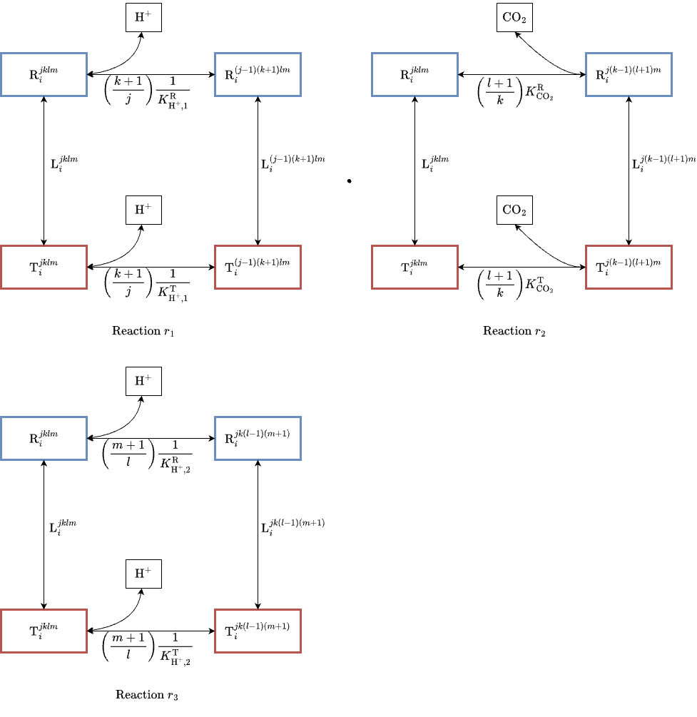
Figure 11: Detailed balance analysis as applied to the allosteric reaction scheme of hemoglobin in relation to the N-terminal group in equation (48) and state transition reaction. Top left figure: Detailed balance loop involving reaction $r_{1}$ (—NH3+ ¡=¿ H+ + —NH2) and allosteric transition R $\leftrightarrow$ T. Top right figure: Detailed balance loop involving reaction $r_{2}$ (—NH2 + CO2 ¡=¿ —NHCOOH) and allosteric transition R $\leftrightarrow$ T. Bottom figure: Detailed balance loop involving reaction $r_{3}$ (—NHCOOH ¡=¿ —NHCOO^- + H+) and allosteric transition R $\leftrightarrow$ T.

$$\begin{cases}\begin{aligned} \text{Reaction}\ r_{1}:\ \left(\dfrac{k+1}{j}\dfrac{1}{K_{\text{H}^{+},1}^{\text{R}}}\right)\left(L_{i}^{jklm}\right)\left(\dfrac{1}{\left(\dfrac{k+1}{j}\right)\dfrac{1}{K_{\text{H}^{+},1}^{\text{R}}}}\right)\left(\dfrac{1}{L_{i}^{(j-1)(k+1)lm}}\right)&=1\end{aligned}\\ \\ \begin{aligned} \text{Reaction}\ r_{2}:\ \left(\dfrac{l+1}{k}K_{\text{CO}_{2}}^{\text{R}}\right)\left(L_{i}^{jklm}\right)\left(\dfrac{1}{\left(\dfrac{l+1}{k}\right)K_{\text{CO}_{2}}^{\text{R}}}\right)\left(\dfrac{1}{L_{i}^{j(k-1)(l+1)m}}\right)&=1\end{aligned}\\ \\ \begin{aligned} \text{Reaction}\ r_{3}:\ \left(\dfrac{m+1}{l}\dfrac{1}{K_{\text{R}^{+},2}^{\text{T}}}\right)\left(L_{i}^{jklm}\right)\left(\dfrac{1}{\left(\dfrac{m+1}{l}\right)\dfrac{1}{K_{\text{H}^{+},2}^{\text{R}}}}\right)\left(\dfrac{1}{L_{i}^{jk(l-1)(m+1)}}\right)&=1\end{aligned}\end{cases}$$

By combining these results with Equation (40), we are able to derive the relationships among the allosteric equilibrium rate constants:

$$\begin{cases}\begin{aligned} \dfrac{L_{i}^{(j-1)(k+1)lm}}{L_{i}^{jklm}}&=\dfrac{K_{\text{H}^{+},1}^{\text{R}}}{K_{\text{H}^{+},1}^{\text{T}}}\\ \end{aligned}\\ \\ \begin{aligned} \dfrac{L_{i}^{j(k-1)(l+1)m}}{L_{i}^{jklm}}&=\dfrac{K_{\text{CO}_{2}}^{\text{R}}}{K_{\text{CO}_{2}}^{\text{T}}}\\ \end{aligned}\\ \\ \begin{aligned} \dfrac{L_{i}^{jk(l-1)(m+1)}}{L_{i}^{jklm}}&=\dfrac{K_{\text{H}^{+},2}^{\text{R}}}{K_{\text{H}^{+},2}^{\text{T}}}\\ \end{aligned}\\ \\ \begin{aligned} L_{i}^{jklm}=\left(\dfrac{K_{\text{H}^{+},1}^{\text{R}}}{K_{\text{H}^{+},1}^{\text{T}}}\right)^{k+l+m}\left(\dfrac{K_{\text{CO}_{2}}^{\text{R}}}{K_{\text{CO}_{2}}^{\text{T}}}\right)^{l+m}\left(\dfrac{K_{\text{H}^{+},2}^{\text{R}}}{K_{\text{H}^{+},2}^{\text{T}}}\right)^{m}L_{i}^{4000}\end{aligned}\\ \\ \begin{aligned} L_{i}^{jklm}=\left(\dfrac{K_{\text{H}^{+},1}^{\text{R}}}{K_{\text{H}^{+},1}^{\text{T}}}\right)^{k+l+m}\left(\dfrac{K_{\text{CO}_{2}}^{\text{R}}}{K_{\text{CO}_{2}}^{\text{T}}}\right)^{l+m}\left(\dfrac{K_{\text{H}^{+},2}^{\text{R}}}{K_{\text{H}^{+},2}^{\text{T}}}\right)^{m}\left(\dfrac{K_{\text{O}_{2}}^{\text{R}}}{K_{\text{O}_{2}}^{\text{T}}}\right)^{i}L_{0}^{4000}\end{aligned}\end{cases}$$

We aim to validate the principle of detailed balance in the context of N-terminal group reactions by examining whether the products of equilibrium constants around the depicted loops in Figure 12 are equal to 1:

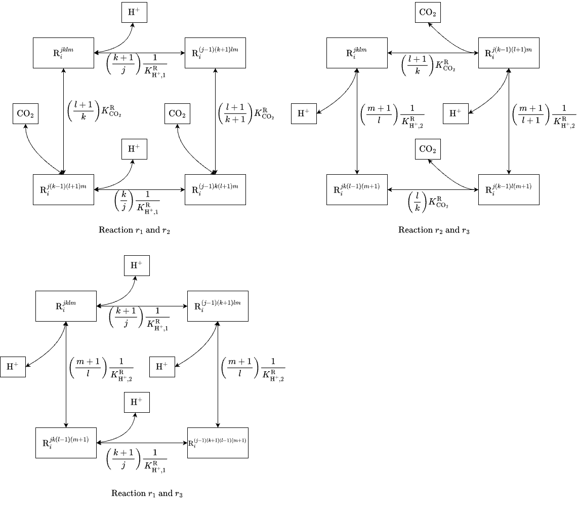
Figure 12: Detailed balance analysis as applied to the allosteric reaction scheme of hemoglobin in relation to the N-terminal group in equation (48). Top left figure: Detailed balance loop involving reaction $r_{1}$ (—NH3+ ¡=¿ H+ + —NH2) and $r_{2}$ (—NH2 + CO2 ¡=¿ —NHCOOH). Top right figure: Detailed balance loop involving reaction $r_{2}$ (—NH2 + CO2 ¡=¿ —NHCOOH) and $r_{3}$ (—NHCOOH ¡=¿ —NHCOO^- + H+). Bottom figure: Detailed balance loop involving reaction $r_{1}$ (—NH3+ ¡=¿ H+ + —NH2) and $r_{3}$ (—NHCOOH ¡=¿ —NHCOO^- + H+).

By checking that the principle of detailed balance is applicable to each reaction, we obtain:

$$\begin{cases}\begin{aligned} \text{Reaction}\ r_{1}\ \text{and}\ r_{2}:\ \left(\dfrac{l+1}{k}K_{\text{CO}_{2}}^{\text{R}}\right)\left(\dfrac{k}{j}\dfrac{1}{K_{\text{H}^{+},1}^{\text{R}}}\right)\left(\dfrac{1}{\dfrac{l+1}{k+1}K_{\text{CO}_{2}}^{\text{R}}}\right)\left(\dfrac{1}{\dfrac{k+1}{j}\dfrac{1}{K_{\text{H}^{+},1}^{\text{R}}}}\right)=1\end{aligned}\\ \\ \begin{aligned} \text{Reaction}\ r_{1}\ \text{and}\ r_{3}:\ \left(\dfrac{m+1}{l}\dfrac{1}{K_{\text{H}^{+},2}^{\text{R}}}\right)\left(\dfrac{k+1}{j}\dfrac{1}{K_{\text{H}^{+},1}^{\text{R}}}\right)\left(\dfrac{1}{\dfrac{m+1}{l}\dfrac{1}{K_{\text{H}^{+},2}^{\text{R}}}}\right)\left(\dfrac{1}{\dfrac{k+1}{j}\dfrac{1}{K_{\text{H}^{+},1}^{\text{R}}}}\right)=1\end{aligned}\\ \\ \begin{aligned} \text{Reaction}\ r_{2}\ \text{and}\ r_{3}:\ \left(\dfrac{m+1}{l}\dfrac{1}{K_{\text{H}^{+},2}^{\text{R}}}\right)\left(\dfrac{l}{k}K_{\text{CO}_{2}}^{\text{R}}\right)\left(\dfrac{1}{\dfrac{m+1}{l+1}\dfrac{1}{K_{\text{H}^{+},2}^{\text{R}}}}\right)\left(\dfrac{1}{\dfrac{l+1}{k}K_{\text{CO}_{2}}^{\text{R}}}\right)=1\end{aligned}\end{cases}$$

Thus all allosteric reactions in N-terminal group subject to the constraints stated in (51) are verified to be in agreement with the principle of detailed balance.

A.2.3 Oxyhemoglobin Saturation

Consider again the reaction diagram provided in Figure 1 along with the reactions defined in (48). To effect the state transition of a single hemoglobin subunit from $\text{Hm---NH}_{3}^{+}$ to $\text{Hm---NHCOO}^{-}$, the subunit must traverse intermediate states $\text{Hm---NH}_{2}$ and Hm—NHCOOH due to the linear reaction scheme. Suppose the reference state of hemoglobin as $\text{R}_{i}^{4000}$. It necessitates $k$ $r_{1}$ reactions to transform into the state $\text{R}_{i}^{(4-k)k00}$; $k$ $r_{1}$ reactions and $k$ $r_{2}$ reactions to convert into the state $\text{R}_{i}^{(4-k)0k0}$; $k$ $r_{1}$ reactions, $k$ $r_{2}$ reactions, and $k$ $r_{3}$ reactions to become the state $\text{R}_{i}^{(4-k)00k}$. Consequently, for any given state $\text{R}_{i}^{jklm}$, it requires a total of (k+l+m) $r_{1}$ reactions, (l+m) $r_{2}$ reactions, and $m$ $r_{3}$ reactions to evolve from the original $\text{R}_{i}^{4000}$ state.

Following the reaction availability argument detailed in section A.1.1 and the three governing reactions outlined in (49), we can derive the following equilibrium state concentration relationships:

$$\dfrac{[\text{R}_{i}^{jk00}]}{[\text{R}_{i}^{4000}]}={4\choose k}\left(\dfrac{K_{\text{H}^{+},1}^{\text{R}}}{[\text{H}^{+}]}\right)^{k}$$

$$\dfrac{[\text{R}_{i}^{jkl0}]}{[\text{R}_{i}^{4000}]}={4\choose k+l}\left(\dfrac{K_{\text{H}^{+},1}^{\text{R}}}{[\text{H}^{+}]}\right)^{k+l}{k+l\choose l}\left(\dfrac{[\text{CO}_{2}]}{K_{\text{CO}_{2}}^{\text{R}}}\right)^{l}$$

$$\dfrac{[\text{R}_{i}^{jklm}]}{[\text{R}_{i}^{4000}]}={4\choose k+l+m}\left(\dfrac{K_{\text{H}^{+},1}^{\text{R}}}{[\text{H}^{+}]}\right)^{k+l+m}{k+l+m\choose l+m}\left(\dfrac{[\text{CO}_{2}]}{K_{\text{CO}_{2}}^{\text{R}}}\right)^{l+m}{l+m\choose m}\left(\dfrac{K_{\text{H}^{+},2}^{\text{R}}}{[\text{H}^{+}]}\right)^{m}$$ (52)

The multinomial coefficients can be simplified as:

$${4\choose k+l+m}{k+l+m\choose l+m}{l+m\choose m}=\dfrac{4!}{j!(k+l+m)!}\dfrac{(k+l+m)!}{k!(l+m)!}\dfrac{(l+m)!}{l!m!}$$

$$=\dfrac{4!}{j!k!l!m!}={4\choose j,k,l,m}$$

The remaining terms of equation (52) can be rewritten and grouped by exponent:

$$\left(\dfrac{K_{\text{H}^{+},1}^{\text{T}}}{[\text{H}^{+}]}\right)^{k+l+m}\left(\dfrac{[\text{CO}_{2}]}{K_{\text{CO}_{2}}^{\text{T}}}\right)^{l+m}\left(\dfrac{K_{\text{H}^{+},2}^{\text{T}}}{[\text{H}^{+}]}\right)^{m}=\left(\dfrac{K_{\text{H}^{+},1}^{\text{T}}}{[\text{H}^{+}]}\right)^{k}\left(\dfrac{K_{\text{H}^{+},1}^{\text{T}}}{[\text{H}^{+}]}\dfrac{[\text{CO}_{2}]}{K_{\text{CO}_{2}}^{\text{T}}}\right)^{l}\left(\dfrac{K_{\text{H}^{+},1}^{\text{T}}}{[\text{H}^{+}]}\dfrac{[\text{CO}_{2}]}{K_{\text{CO}_{2}}^{\text{T}}}\dfrac{K_{\text{H}^{+},2}^{\text{T}}}{[\text{H}^{+}]}\right)^{m}$$

Thus we have

$$\dfrac{[\text{R}_{i}^{jklm}]}{[\text{R}_{i}^{4000}]}={4\choose j,k,l,m}\left(\dfrac{K_{\text{H}^{+},1}^{\text{R}}}{[\text{H}^{+}]}\right)^{k}\left(\dfrac{K_{\text{H}^{+},1}^{\text{R}}}{[\text{H}^{+}]}\dfrac{[\text{CO}_{2}]}{K_{\text{CO}_{2}}^{\text{R}}}\right)^{l}\left(\dfrac{K_{\text{H}^{+},1}^{\text{R}}}{[\text{H}^{+}]}\dfrac{[\text{CO}_{2}]}{K_{\text{CO}_{2}}^{\text{R}}}\dfrac{K_{\text{H}^{+},2}^{\text{R}}}{[\text{H}^{+}]}\right)^{m}$$ (53)

Further applying equation (42), we can determine the equilibrium concentration of any arbitrary state relative to the reference state. For any R state:

$$\dfrac{[\text{R}_{i}^{jklm}]}{[\text{R}_{0}^{4000}]}={4\choose i}\left(\dfrac{[\text{O}_{2}]}{K_{\text{O}_{2}}^{\text{R}}}\right)^{i}{4\choose j,k,l,m}\left(\dfrac{K_{\text{H}^{+},1}^{\text{R}}}{[\text{H}^{+}]}\right)^{k}\left(\dfrac{K_{\text{H}^{+},1}^{\text{R}}}{[\text{H}^{+}]}\dfrac{[\text{CO}_{2}]}{K_{\text{CO}_{2}}^{\text{R}}}\right)^{l}\left(\dfrac{K_{\text{H}^{+},1}^{\text{R}}}{[\text{H}^{+}]}\dfrac{[\text{CO}_{2}]}{K_{\text{CO}_{2}}^{\text{R}}}\dfrac{K_{\text{H}^{+},2}^{\text{R}}}{[\text{H}^{+}]}\right)^{m}$$ (54)

Similarly, for any T state:

$$\dfrac{[\text{T}_{i}^{jklm}]}{[\text{T}_{0}^{4000}]}={4\choose i}\left(\dfrac{[\text{O}_{2}]}{K_{\text{O}_{2}}^{\text{T}}}\right)^{i}{4\choose j,k,l,m}\left(\dfrac{K_{\text{H}^{+},1}^{\text{T}}}{[\text{H}^{+}]}\right)^{k}\left(\dfrac{K_{\text{H}^{+},1}^{\text{T}}}{[\text{H}^{+}]}\dfrac{[\text{CO}_{2}]}{K_{\text{CO}_{2}}^{\text{T}}}\right)^{l}\left(\dfrac{K_{\text{H}^{+},1}^{\text{T}}}{[\text{H}^{+}]}\dfrac{[\text{CO}_{2}]}{K_{\text{CO}_{2}}^{\text{T}}}\dfrac{K_{\text{H}^{+},2}^{\text{T}}}{[\text{H}^{+}]}\right)^{m}$$ (55)

Given the equilibrium state relation:

$$[\text{R}_{0}^{4000}]L_{0}^{4000}=[\text{T}_{0}^{4000}]$$

we find that:

$$\dfrac{[\text{R}_{0}^{4000}]}{[\text{T}_{0}^{4000}]}=\dfrac{1}{L_{0}^{4000}}$$ (56)

The state of hemoglobin and the concentration of bound oxygen can be expressed in terms of $[\text{T}_{0}^{4000}]$, enabling us to determine the total hemoglobin concentration $[\text{Hb}^{*}]$ and the total bound oxygen concentration $[\text{O}2]_{\text{bound}}$:

$$\begin{cases}\begin{aligned} &=\sum_{i=0}^{4}\sum_{j+k+l+m=4}[\text{R}_{i}^{jklm}]+\sum_{i=0}^{4}\sum_{j+k+l+m=4}[\text{T}_{i}^{jklm}]\\ &=[\text{T}_{0}^{4000}]\dfrac{1}{L_{0}^{4000}}\left(1+\dfrac{[\text{O}_{2}]}{K_{\text{O}_{2}}^{\text{R}}}\right)^{4}\left(1+\dfrac{K_{\text{H}^{+},1}^{\text{R}}}{[\text{H}^{+}]}\left(1+\dfrac{[\text{CO}_{2}]}{K_{\text{CO}_{2}}^{\text{R}}}\left(1+\dfrac{K_{\text{H}^{+},2}^{\text{R}}}{[\text{H}^{+}]}\right)\right)\right)^{4}+\\ &[\text{T}_{0}^{4000}]\left(1+\dfrac{[\text{O}_{2}]}{K_{\text{O}_{2}}^{\text{T}}}\right)^{4}\left(1+\dfrac{K_{\text{H}^{+},1}^{\text{T}}}{[\text{H}^{+}]}\left(1+\dfrac{[\text{CO}_{2}]}{K_{\text{CO}_{2}}^{\text{T}}}\left(1+\dfrac{K_{\text{H}^{+},2}^{\text{T}}}{[\text{H}^{+}]}\right)\right)\right)^{4}\end{aligned}\\ \\ \begin{aligned} {}_{\text{bound}}&=\sum_{i=0}^{4}\sum_{j+k+l+m=4}i[\text{R}_{i}^{jklm}]+\sum_{i=0}^{4}\sum_{j+k+l+m=4}i[\text{T}_{i}^{jklm}]\\ &=4[\text{T}_{0}^{4000}]\dfrac{1}{L_{0}^{4000}}\dfrac{[\text{O}_{2}]}{K_{\text{O}_{2}}^{\text{R}}}\left(1+\dfrac{[\text{O}_{2}]}{K_{\text{O}_{2}}^{\text{R}}}\right)^{3}\left(1+\dfrac{K_{\text{H}^{+},1}^{\text{R}}}{[\text{H}^{+}]}\left(1+\dfrac{[\text{CO}_{2}]}{K_{\text{CO}_{2}}^{\text{R}}}\left(1+\dfrac{K_{\text{H}^{+},2}^{\text{R}}}{[\text{H}^{+}]}\right)\right)\right)^{4}+\\ &4[\text{T}_{0}^{4000}]\dfrac{[\text{O}_{2}]}{K_{\text{O}_{2}}^{\text{T}}}\left(1+\dfrac{[\text{O}_{2}]}{K_{\text{O}_{2}}^{\text{T}}}\right)^{3}\left(1+\dfrac{K_{\text{H}^{+},1}^{\text{T}}}{[\text{H}^{+}]}\left(1+\dfrac{[\text{CO}_{2}]}{K_{\text{CO}_{2}}^{\text{T}}}\left(1+\dfrac{K_{\text{H}^{+},2}^{\text{T}}}{[\text{H}^{+}]}\right)\right)\right)^{4}\end{aligned}\end{cases}$$ (57)

Further, we can define:

$$\widetilde{L}_{0}^{4000}=\dfrac{L_{0}^{4000}\left(1+\dfrac{K_{\text{H}^{+},1}^{\text{R}}}{[\text{H}^{+}]}\left(1+\dfrac{[\text{CO}_{2}]}{K_{\text{CO}_{2}}^{\text{R}}}\left(1+\dfrac{K_{\text{H}^{+},2}^{\text{R}}}{[\text{H}^{+}]}\right)\right)\right)^{4}}{\left(1+\dfrac{K_{\text{H}^{+},1}^{\text{T}}}{[\text{H}^{+}]}\left(1+\dfrac{[\text{CO}_{2}]}{K_{\text{CO}_{2}}^{\text{T}}}\left(1+\dfrac{K_{\text{H}^{+},2}^{\text{T}}}{[\text{H}^{+}]}\right)\right)\right)^{4}}$$ (58)

similar to (26), so that (57) can be rewritten as

$$\begin{cases}\begin{aligned} =[\text{T}_{0}^{4000}]\left(1+\dfrac{K_{\text{H}^{+},1}^{\text{R}}}{[\text{H}^{+}]}\left(1+\dfrac{[\text{CO}_{2}]}{K_{\text{CO}_{2}}^{\text{R}}}\left(1+\dfrac{K_{\text{H}^{+},2}^{\text{R}}}{[\text{H}^{+}]}\right)\right)\right)^{4}\\ \\ \left(\dfrac{1}{\widetilde{L}_{0}^{4000}}\left(1+\dfrac{[\text{O}_{2}]}{K_{\text{O}_{2}}^{\text{R}}}\right)^{4}+\left(1+\dfrac{[\text{O}_{2}]}{K_{\text{O}_{2}}^{\text{T}}}\right)^{4}\right)\end{aligned}\\ \\ \begin{aligned} {}_{\text{bound}}=4[\text{T}_{0}^{4000}]\left(1+\dfrac{K_{\text{H}^{+},1}^{\text{R}}}{[\text{H}^{+}]}\left(1+\dfrac{[\text{CO}_{2}]}{K_{\text{CO}_{2}}^{\text{R}}}\left(1+\dfrac{K_{\text{H}^{+},2}^{\text{R}}}{[\text{H}^{+}]}\right)\right)\right)^{4}\\ \\ \left(\dfrac{1}{\widetilde{L}_{0}^{4000}}\dfrac{[\text{O}_{2}]}{K_{\text{O}_{2}}^{\text{R}}}\left(1+\dfrac{[\text{O}_{2}]}{K_{\text{O}_{2}}^{\text{R}}}\right)^{3}+\dfrac{[\text{O}_{2}]}{K_{\text{O}_{2}}^{\text{T}}}\left(1+\dfrac{[\text{O}_{2}]}{K_{\text{O}_{2}}^{\text{T}}}\right)^{3}\right)\end{aligned}\end{cases}$$ (59)

Then,

$$S_{\text{O}_{2}}=\dfrac{[\text{O}_{2}]_{\text{bound}}}{4[\text{Hb}^{*}]}=\dfrac{\dfrac{1}{\widetilde{L}_{0}^{4000}}\dfrac{[\text{O}_{2}]}{K_{\text{O}_{2}}^{\text{R}}}\left(1+\dfrac{[\text{O}_{2}]}{K_{\text{O}_{2}}^{\text{R}}}\right)^{3}+\dfrac{[\text{O}_{2}]}{K_{\text{O}_{2}}^{\text{T}}}\left(1+\dfrac{[\text{O}_{2}]}{K_{\text{O}_{2}}^{\text{T}}}\right)^{3}}{\dfrac{1}{\widetilde{L}_{0}^{4000}}\left(1+\dfrac{[\text{O}_{2}]}{K_{\text{O}_{2}}^{\text{R}}}\right)^{4}+\left(1+\dfrac{[\text{O}_{2}]}{K_{\text{O}_{2}}^{\text{T}}}\right)^{4}}$$ (60)

This is the same as (27). The result here has been derived by chemical-kinetic reasoning, whereas (27) was derived by probabilistic reasoning.

Appendix B Conversion between Molar Concentrations and Partial Pressures for $\text{O}_{2}$ and $\text{CO}_{2}$, and between Molar Concentration and pH for $\text{H}^{+}$; with a Remark on the Significance of these Independent Variables.

In the formulation of our model, we use the free molar concentrations of $\text{O}_{2}$, $\text{CO}_{2}$, and $\text{H}^{+}$ as our independent variables. The word ”free” in this context means not bound to hemoglobin (or to anything else). In the experimental literature, the corresponding values that are stated are usually the partial pressures of $\text{O}_{2}$ and $\text{CO}_{2}$, and the pH.

The conversion between free molar concentration and partial pressure is given by Henry’s law: [$\text{O}_{2}$] = $\alpha_{\text{O}_{2}}\text{P}_{\text{O}_{2}}$ and [$\text{CO}_{2}$] = $\alpha_{\text{CO}_{2}}\text{P}_{\text{CO}_{2}}$. Here, $\alpha_{\text{O}_{2}}$ and $\alpha_{\text{CO}_{2}}$ represent the solubility of oxygen and carbon dioxide in water, respectively.

Under physiological conditions, characterized by normal body temperature, the values of $\alpha_{\text{O}_{2}}$ and $\alpha_{\text{CO}_{2}}$ are known to be $1.46\times 10^{-6}$ M $\text{mmHg}^{-1}$ and $3.27\times 10^{-5}$ M $\text{mmHg}^{-1}$, respectively. These values were derived from the experimental data procured from Austin et al. (1963) for $\alpha{\text{O}_{2}}$ and Hedley-Whyte and Lave (1964) for $\alpha_{\text{CO}_{2}}$.

Finally, the conversion between [$\text{H}^{+}$] and pH is given by the definition of pH, which is pH = $-log_{10}[\text{H}^{+}$].

An important remark is that by controlling the free concentrations of $\text{O}_{2}$, $\text{CO}_{2}$, and $\text{H}^{+}$, we eliminate the need to consider the physiologically important reaction

$$\ce{H2O+CO2<=>H2CO3<=>HCO3-+H+}$$ (61)

through which the $\text{CO}_{2}$ and $\text{H}^{+}$ interact. Likewise, we avoid the need to worry about the influence of binding to hemoglobin on the free concentrations themselves. These considerations will become important, however, in the physiological application of our model.

References

- [1] Alberty, R. A. (2004). Principle of detailed balance in kinetics. Journal of Chemical Education, 81(8), 1206.
- [2] Antonini, E. (1971). Hemoglobin and myoglobin in their reactions with ligands. Frontiers of biology, 21, 27-31.
- [3] Austin, W. H., Lacombe, E., Rand, P. W., & Chatterjee, M. (1963). Solubility of carbon dioxide in serum from 15 to 38 C. Journal of Applied Physiology, 18(2), 301-304.
- [4] Buerk, D. G., & Bridges, E. W. (1986). A simplified algorithm for computing the variation in oxyhemoglobin saturation with pH, PCO2, T and DPG. Chemical Engineering Communications, 47(1-3), 113-124.
- [5] Dash, R. K., & Bassingthwaighte, J. B. (2010). Erratum to: Blood HbO2 and HbCO2 dissociation curves at varied O2, CO2, pH, 2, 3-DPG and temperature levels. Annals of biomedical engineering, 38(4), 1683-1701.
- [6] Dash, R. K., Korman, B., & Bassingthwaighte, J. B. (2016). Simple accurate mathematical models of blood HbO 2 and HbCO 2 dissociation curves at varied physiological conditions: evaluation and comparison with other models. European journal of applied physiology, 116, 97-113.
- [7] Hamby D. M. (1994). A review of techniques for parameter sensitivity analysis of environmental models. Environmental monitoring and assessment, 32(2), 135–154. https://doi.org/10.1007/BF00547132
- [8] Hedley-Whyte, J., & Laver, M. B. (1964). O2 solubility in blood and temperature correction factors for PO2. Journal of Applied Physiology, 19(5), 901-906.
- [9] Hill, A. V. (1910). The possible effects of the aggregation of the molecules of hemoglobin on its dissociation curves. j. physiol., 40, iv-vii.
- [10] Hopfield, J.J., Shulman, R.G., & Ogawa, S. (1971). An allosteric model of hemoglobin: I, kinetics. Journal of Molecular Biology, 55(4), 533-557.
- [11] Hsia, C. C. (1998). Respiratory function of hemoglobin. New England Journal of Medicine, 338(4), 239-248.
- [12] Imamura, T. (1996). Human hemoglobin structure and respiratory transport. Nihon rinsho. Japanese Journal of Clinical Medicine, 54(9), 2320-2325.
- [13] Joels, N., & Pugh, L. G. C. E. (1958). The carbon monoxide dissociation curve of human blood. The Journal of Physiology, 142(1), 63.
- [14] Kelman, G. R. (1966). Digital computer subroutine for the conversion of oxygen tension into saturation. Journal of applied physiology, 21(4), 1375-1376.
- [15] Kilmartin, J. V., & Rossi-Bernardi, L. (1973). Interaction of hemoglobin with hydrogen ions, carbon dioxide, and organic phosphates. Physiological reviews, 53(4), 836-890.
- [16] Marengo-Rowe, A. J. (2006, July). Structure-function relations of human hemoglobins. In Baylor University Medical Center Proceedings (Vol. 19, No. 3, pp. 239-245). Taylor & Francis.
- [17] Monod J, Wyman J, & Changeux J.P. (1965). On the nature of allosteric transitions: a plausible model. J Mol Biol, 12(1), 88-118.
- [18] Pittman, R. N. (2016). Regulation of tissue oxygenation.
- [19] Royer, W.E., Zhu, H., Gorr, T.A., & Flores, J.F. (2005). Allosteric hemoglobin assembly: diversity and similarity. Journal of Biological Chemistry, 280(27), 24978-24981.
- [20] Salathé, E. P., Fayad, R., & Schaffer, S. W. (1981). Mathematical analysis of carbon dioxide transport by blood. Mathematical Biosciences, 57(1-2), 109-153.
- [21] Shibayama, N. (2020). Allosteric transitions in hemoglobin revisited. Biochimica et Biophysica Acta (BBA)-General Subjects, 1864(12), 129694.
- [22] Siggaard-Andersen, O., Wimberley, P. D., Göthgen, I., & Siggaard-Andersen, M. (1984). A mathematical model of the hemoglobin-oxygen dissociation curve of human blood and of the oxygen partial pressure as a function of temperature. Clinical chemistry, 30(10), 1646-1651.
- [23] Singh, M. P., Sharan, M., & Aminataei, A. (1989). Development of mathematical formulae for O2 and CO2 dissociation curves in the blood. Mathematical Medicine and Biology: A Journal of the IMA, 6(1), 25-46.
- [24] Winslow, R. M., Swenberg, M. L., Berger, R. L., Shrager, R. I., Luzzana, M., Samaja, M., & Rossi-Bernardi, L. (1977). Oxygen equilibrium curve of normal human blood and its evaluation by Adair’s equation. Journal of Biological Chemistry,252(7), 2331-2337.
- [25] Woyke, S., Brugger, H., Ströhle, M., Haller, T., Gatterer, H., Dal Cappello, T., & Strapazzon, G. (2022). Effects of carbon dioxide and temperature on the oxygen-hemoglobin dissociation curve of human blood: Implications for avalanche victims. Frontiers in medicine, 8, 808025.
- [26] Wyman, J. (1963). Allosteric effects in hemoglobin. Cold Spring Harbor Symposia on Quantitative Biology, 28, 355-365.