Wavelet Scattering Transform for Bioacustics: Application to Watkins Marine Mammal Sound Database

Abstract

Marine mammal communication is a complex field, hindered by the diversity of vocalizations and environmental factors. The Watkins Marine Mammal Sound Database (WMMD) is an extensive labeled dataset used in machine learning applications. However, the methods for data preparation, preprocessing, and classification found in the literature are quite disparate. This study first focuses on a brief review of the state-of-the-art benchmarks on the dataset, with an emphasis on clarifying data preparation and preprocessing methods. Subsequently, we propose the application of the Wavelet Scattering Transform (WST) in place of standard methods based on the Short-Time Fourier Transform (STFT). The study also tackles a classification task using an ad-hoc deep architecture with residual layers. We outperform the existing classification architecture by $6\%$ in accuracy using WST and $8\%$ using Mel spectrogram preprocessing, effectively reducing by half the number of misclassified samples, and reaching a top accuracy of $96\%$.

1 Introduction

Marine mammals, which include species like whales, dolphins, and seals, are celebrated for their intricate communication systems crucial for survival and social interactions. Despite the significance of these communication systems, understanding them remains challenging due to the diverse range of vocalizations, behaviors, and environmental factors involved (Watkins & Wartzok, 1985)(Dudzinski et al., 2009). Recent research efforts have increasingly turned towards harnessing machine learning (ML) to analyze and decipher communication patterns among marine mammals (Mazhar et al., 2007) (Bermant et al., 2019). The application of AI and ML enables researchers to classify vocalizations effectively, monitor movements, and gain insights into behavior and social structures (Mustill, 2022). Additionally, these technologies support ecological studies by correlating whale vocalizations with environmental factors, providing valuable insights into behavioral patterns and social structures. Real-time monitoring establishes early warning systems for conservation efforts, helping mitigate the impact of human activities on whale populations (Croll et al., 2001)(Gibb et al., 2019).
A significant resource in the study of marine mammal communication is the Watkins Marine Mammal Sound Database (WMMD) (Sayigh et al., 2016). Spanning seven decades, this collection of recordings encompasses various marine mammal species and holds immense historical and scientific value. While the WMMD serves as a renowned reference dataset for studying vocalizations, it presents challenges for classification, including variability and complexity in vocalizations, environmental noise, and data scarcity for certain species.
Current state-of-the-art benchmarks heavily rely on deep learning (Ghani et al., 2023) or peculiar data preparation and preprocessing (Murphy et al., 2022)(Hagiwara et al., 2023)(Hagiwara, 2023). Moreover, most of current works usually tackle just portion of the full dataset, as for instance very few classes (Lu et al., 2021) or the ”best of” subset (Hagiwara et al., 2023). Moreover, the main preprocessing methods are based on Short Time Fourier Transform (Roberts & Mullis, 1987) and further specifications. Addressing these issues, we introduce the Wavelet Scattering Transform (WST) (Mallat, 2012)(Bruna & Mallat, 2013) in our work. Regarded as the mathematical counterpart of Convolutional layers in deep networks, WST boasts invariance and stability properties concerning signal translation and deformation—qualities absent in standard preprocessing. Furthermore, the structure of the scattering coefficients proves valuable in providing a physical interpretation of multiscale processes, especially in the context of complex natural sounds (Khatami et al., 2018).
The significance of the dataset extends beyond biology, representing a noteworthy example of natural time series. Preprocessing and statistics of such objects present a longstanding challenge in data science from the early methods based on Fourier analysis to modern AI-based tools (Fu, 2011)(Aghabozorgi et al., 2015). WST has found application in various physical datasets, contributing to advancements in understanding multiscale and multifrequency processes that are challenging to address with standard Fourier techniques (Bruna & Mallat, 2019)(Cheng et al., 2020)(Glinsky et al., 2020).
In this study we focus on WMMD and:

• we collect a review of data preparation, preprocessing and classification methods used in literature which can be potentially important for bioacustics community;

• we provide a novel detailed and public pipeline for data preparation of WMMD, with the accent on the use of WST as alternative preprocessing method;

• we propose a deep architecture with residual layers, demonstrating higher classification accuracy compared to existing benchmarks for both WST and standard preprocessing.

In Table 1 we report a short summary of accuracy results for classification task, as opposed to existing benchmarks. The code for the present work is available at the public GitHub repository wmmd_vocalization_classification.

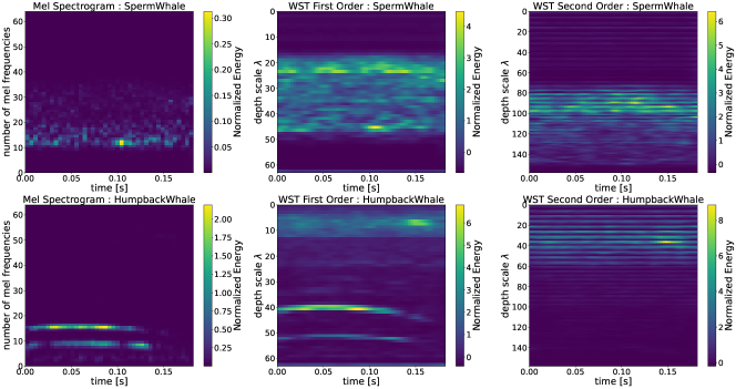
Figure 1: From left: Mel spectrogram, WST of first and second order for vocalizations of two different species of whales. The displayed WSTs correspond to the choice $(J,Q)=(7,10)$. Focusing on the second row, it is graphically evident the correspondence of high depth scale for WST with low frequency in the spectrogram. Mel spectrogram appears to be more coarse-grained with respect to first-order WST, even if the overall heatmaps appear to be similar. Each figure is resized to be squared for visualization purposes. The shapes of the images in each row are, from left, respectively 41$\times$64 for Mel spectrogram and 53$\times$63 and 158$\times$63 for first and second order WST.

2 Preprocessing techniques

2.1 STFT and Mel Spectrogram

Spectrogram representation is one of the most common technique used in 1D signal representation theory, cfr. (Roberts & Mullis, 1987). It provides information about the energy spectrum in the time-frequency domain $(t,\omega)$ and it is based on the Short Time Fourier Transform (STFT). Let us briefly recall the definition of STFT: we suppose that the time variable $t$ is a positive real number, i.e. $t\in[0,+\infty)$. Let us fix a function $h(t)$ called window function, most common choices being Hann window or Gaussian window. Hann window, with support length $T>0$, has the following form

$$h(t)=a\cos^{2}\left(\frac{\pi t}{T}\right)\mathbf{1}_{\{|t|\leq T/2\}}(t)\,$$ (1)

while Gaussian window is a centered Gaussian function with amplitude $a$ and spread $\sigma$, i.e.

$$h(t)=a\exp\left(-\frac{t^{2}}{2\sigma^{2}}\right)\,.$$ (2)

As one can infer from the name, a window function is usually chosen to be localized in time domain, and can also be compactly supported as (1). We can then recall the following definition:

Definition 2.1.

For a given signal $x(t)$ and a fixed window function $h(t)$, the Short Time Fourier Transform is defined as

$$\mathbf{STFT}\{x\}(t,\omega)=\int_{-\infty}^{\infty}x(\tau)h(\tau-t)e^{-i\omega\tau}\,d\tau.$$ (3)

Note that STFT is strictly related to the Fourier transform operator $\mathcal{F}$, due to the immediate relation

$$\mathbf{STFT}\{x\}(t,\omega)=\mathcal{F}\{x(\tau)h(\tau-t)\}(\omega)$$ (4)

i.e. the Fourier transform of the signal $x(\tau)$ multiplied by a moving window $h(\tau-t)$, for any $t>0$. A trivial extension of the definition to the discrete time case is possible, by replacing the integral with an infinite summation. Given the STFT we recall the definition of spectrogram

Definition 2.2.

For any $t>0$ and $\omega>0$, and for a chosen window $h(t)$ the spectrogram of a signal $x$ is defined as the power spectrum of $x(\tau)h(\tau-t)$, i.e.

$$|X(t,\omega)|^{2}=|\mathbf{STFT}\{x\}(t,\omega)|^{2}\,,$$ (5)

The Mel spectrogram (Rabiner & Schafer, 2010), often employed in audio signal processing, involves a transformation of the spectrogram introduced in Definition (2.2) to a Mel frequency scale. This scale is designed to mimic the human ear’s non-linear frequency perception. For a given signal $x(t)$ and a chosen window function $h(t)$, the Mel spectrogram is defined as the power spectrum of the signal transformed to the Mel frequency scale. It provides a detailed representation of the signal’s energy distribution across both time and Mel frequency variables. The first step in computing the Mel spectrogram involves defining a set of triangular filters, often referred to as the Mel filter bank. These filters are spaced along the Mel frequency scale and overlap to capture the non-uniform nature of human hearing. This scaling choice is well motivated for natural sounds and has been used for preprocessing since the first application to classification of labelled sounds (Lee et al., 2006). Informally, an analysis of signal that is based of an ear-like preprocessing should simplify classification.
Let $N$ be the number of filters in the Mel filter bank, and $f(m)$ be the center frequency of the $m$-th filter. The Mel frequency $m$ corresponding to a given frequency $\omega$ is computed using the formula:

$$m=2595\cdot\log_{10}\left(1+\frac{\omega}{700}\right).$$ (6)

The center frequency $f(m)$ in Hertz corresponding to a Mel frequency $m$ is then given by:

$$f(m)=700\cdot(10^{m/2595}-1).$$ (7)

Each triangular filter $H_{m}(\omega)$ is defined as

$$H_{m}(\omega)=\begin{cases}0&\text{if }\omega<f(m-1)\\ \frac{\omega-f(m-1)}{f(m)-f(m-1)}&\text{if }f(m-1)\leq\omega\leq f(m)\\ 1-\frac{\omega-f(m)}{f(m+1)-f(m)}&\text{if }f(m)\leq\omega\leq f(m+1)\\ 0&\text{if }\omega>f(m+1)\end{cases}$$ (8)

The Mel spectrogram is computed by summing the energy in each triangular filter bank applied to the magnitude of the Short Time Fourier Transform (STFT) of the signal:

$$\text{Mel Spectrogram}(t,m)=\sum_{k=0}^{N-1}|X(t,\omega_{k})|^{2}\cdot H_{m}(\omega_{k}),$$ (9)

where $N$ is the number of frequency bins in the STFT, $X(t,\omega_{k})$ is the STFT magnitude at time $t$ and frequency bin $\omega_{k}$, and $H_{m}(\omega_{k})$ is the value of the $m$-th Mel filter at frequency bin $\omega_{k}$.

2.2 Wavelet Scattering Transform

The Wavelet Scattering Transform (WST) (Mallat, 2012) stands as a mathematical operator capable of yielding a stable and invariant representation for a given signal. Specifically, when certain conditions are met (Bruna & Mallat, 2013), the resulting representation exhibits translation invariance, resistance to additive noise (i.e., it remains non-expansive), and stability to deformations. The latter property is formally expressed as Lipschitz-continuity under the influence of $C^{2}$-diffeomorphisms in its original derivation. Integrating a representation operator with these advantageous characteristics into a machine learning framework has the potential to significantly reduce the computational burden involved in training classification algorithms (Bruna, 2013). Since its derivation has been proposed very recently, in this section we provide an extended summary of definition and properties of WST for 1D signals (n.b. an extension to higher dimensions can be found for instance in (Bruna & Mallat, 2013)).
Let $\psi\in L^{2}(\mathbb{R},dx)$ be a function, called mother wavelet, for a fixed scale factor $a>1$ and for any $j\in\mathbb{Z}$, the $j-$th wavelet is defined as

$$\psi_{a^{j}}(t)=a^{-j}\psi(a^{-j}t)$$ (10)

Let $\lambda=a^{j}$ be the scaling-rotation operator, (10) can be redefined in terms of $\lambda$ as

$$\psi_{\lambda}(t)=\lambda^{-1}\psi(\lambda^{-1}t)\,.$$ (11)

To build an intuitive connection with STFT, $a$ is analogous to the width used for Hann or Gaussian windows. About the choice of the mother wavelet, we refer in the following to Morlet wavelet (Mallat, 1999). In practice, in the usual definition of WST they define $Q\in\mathbb{N}$ such that $a=2^{1/Q}$; this will play a role of hyperparameter.
In order to construct the wavelet scattering operator we fix the so-called depth $J\in\mathbb{N}$ and let $\Lambda_{J}=\{\lambda=a^{j}\,:|\lambda|=a^{j}\leq 2^{J}\}$ be the set of scattering indexes. Then, we introduce a scaled low-pass filter $\phi_{J}(t)=2^{-J}\phi(2^{-J}t)$, where $\phi(t)$ is a Gaussian $\mathcal{N}(0,\sigma^{2})$ with $\sigma=0.7$, and a path $p=(\lambda_{1},\dots.\lambda_{m})$, $\lambda_{i}\in\Lambda_{J}$ which is any tuple of length $m$ build using the scattering indexes; the wavelet scattering coefficient along a path $p$ is defined as

$$S_{J}[p]x(u)=U[p]x\star\phi_{J}(t)=\int_{-\infty}^{\infty}U[p]x(\tau)\phi_{J}(t-\tau)d\tau\,,$$ (12)

where

$$U[p]x=U[\lambda_{m}]\dots U[\lambda_{1}]x=|\dots|x\star\psi_{\lambda_{1}}|\star\psi_{\lambda_{2}}|\dots|\star\psi_{\lambda_{m}}|\,.$$ (13)

For the conducted experiments we couple Morlet wavelets with a Gaussian low-pass filter (Mallat, 1999).
Let us clarify the definition of WST in layman’s terms: by a simple combinatorial argument, the longer is the path, the bigger is the number of combinations of scattering indexes, and more precisely one has the characteristic tree structure, as one can see in Figure 2. Each black dot corresponds to a scattering coefficient and one usually refers to the coefficient for fixed $m$ as the $m$-order scattering coefficients. In analogy with the spectrogram representation, it is usual to plot the coefficients of the same order on a single heatmap, having time and $j$ on the axis, see Figure 1. Notice how $J$ is another free hyperparameter whose effect is to increase the cardinality of $\Lambda_{J}$ hence the number of coefficients per order. To practically infer the importance of the order, following (Mallat, 2012) we introduce the path set up to length $m$, $\Lambda_{J}^{m}=\{(\lambda_{1},\dots,\lambda_{m}):\,|\lambda_{i}|=a^{j}\leq 2^{J}\}$, it is possible to define the induced norm of the scattering operator over the set $\mathcal{P}_{J}=\bigcup\Lambda_{J}^{m}$, i.e.

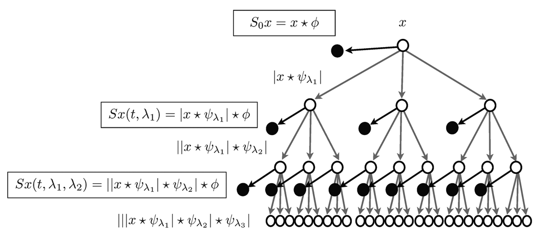
Figure 2: Wavelet Scattering Transform as an iterative process; image taken from (Andén & Mallat, 2014). In their notation the signal is $x(t)=h(t)$ the path $p$ at depth $m$ is explicited in parentheses as a tuple $(\lambda_{1},\dots,\lambda_{m})$. Each black dot corresponds to a scattering coefficient.

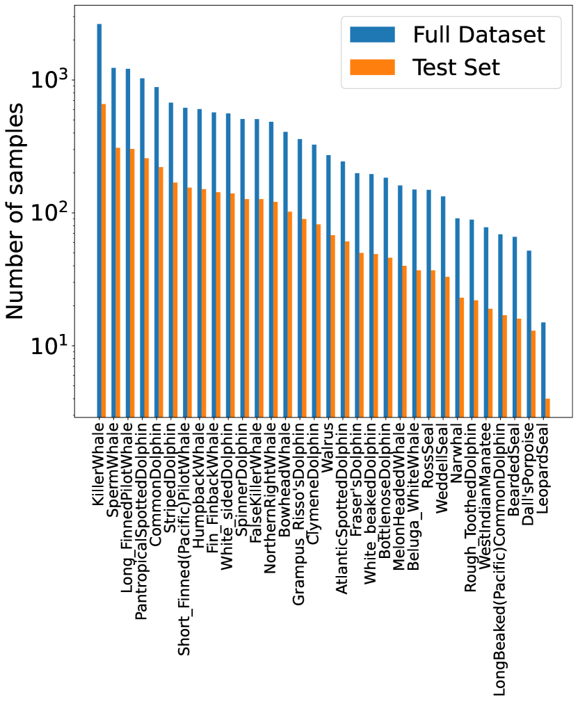
Figure 3: Number of samples per class after data preparation and elimination of duplicates, in log-scale and sorted in decreasing order. The dataset is very imbalanced: the most represented class contains $2637$ instances, while the smallest one just $15$.

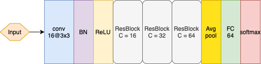
Figure 4: Structure of the architecture employed in the classification task. The residual blocks are unfolded in Figure 5. The acronym ”BN” stands for batch normalization, while ”FC 64” denotes a fully connected layer with input dimension $64$ and output dimension $32$, corresponding to the number of classes. The number of trainable parameters is $176400$.

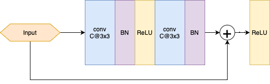
Figure 5: Structure of the residual block used in the full architecture 4. The acronym ”BN” stands for batch normalization.

$$\|S_{J}[\mathcal{P}_{J}]x\|=\sum_{p\in\mathcal{P}_{J}}\|S_{J}[p]x\|$$ (14)

where $\|\cdot\|$ stands for the $L^{2}-$norm. For fixed $J$ and $Q$, and given the definition of $\Lambda_{J}^{m}$. One could be concerned about the depth requested in practice, but in different experiment (Bruna, 2013) it has been showed that just $2$ or $3$ orders, also referred to as layers, of WST are sufficient to represent around $98\%$ of the energy of the signal. Indeed the energy of each layer, i.e. $\|U[\Lambda_{J}^{m}]\|$, is empirically observed to rapidly converge to zero. Thus, usually no more than two orders need to be computed to capture most of the information contained in the signal.

3 Experiments and Results

In this section, our objective is to conduct a comprehensive comparison of the data analysis between the Mel spectrogram and the WST. We emphasize that the pipeline for this comparison is entirely general and could potentially be extended to any temporal series. Notably, the application of WST as a theoretical tool is already prevalent in diverse fields such as cosmology (Valogiannis & Dvorkin, 2022) and field theory (Marchand et al., 2022). As a widely acknowledged principle in the literature (Bruna & Mallat, 2013), WST is preferable to STFT methods when their performances are comparable, primarily due to the invariance properties that facilitate cross-signal interpretation.
Regarding practical computations, the Mel spectogram is calculated using Torchaudio python library, while for WST we used Kymatio python library (Andreux et al., 2020). Training of the networks is conducted on GPUs, specifically RTX8000 NVIDIA (New York University HPC) and Apple M1 chip GPU (personal computer).

3.1 Data Preparation and Preprocessing

The dataset comprises 15,554 samples collected over 70 years by the Woods Hole Oceanographic Institution (Sayigh et al., 2016), representing sounds produced by 51 marine mammal species. Challenges in the dataset include data heterogeneity due to different sensors and class-wise imbalance, leading us to follow the approach in (Bach et al., 2023) by excluding classes with fewer than 50 samples, reducing the species to 32. A detailed examination revealed over 300 repeated samples, some with different labels. Consequently, we removed duplicate signals, resulting in 14,767 unique signals. To address varying signal lengths, we aligned and centered them, fixing the number of time stamps at 8,000. Signals longer than 8,000 retained central points, while shorter ones were padded with equal zeros on both sides. Post data preparation, each signal was standardized, ensuring zero sample mean and unitary variance. With a sample rate of 43,900 Hz, we employed a time window of 0.182 seconds. This length is significantly shorter with respect to related works in mammal vocalizations (Murphy et al., 2022; Ghani et al., 2023), yielding less memory and computational overload for storing the signals and for preprocessing.

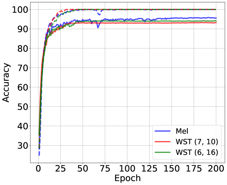
Figure 6: Accuracy per epoch for Mel spectrogram and WST with three couples of $(J,Q)$. Batch size of $128$. Solid line: accuracy on test set. Dashed line: training accuracy.

Regarding the preprocessing, we experimented different combinations of WST hyperparameters, specifically the depth scale parameter $J$ and the resolution $Q$ (where $(J,Q)\in\{(7,10),(6,16)\}$), capturing diverse signal information. The choice $(6,16)$ is adapted to the human ear frequency band, as used for Free Spoken Digits classification (Andreux et al., 2020). The zero-th order WST, providing no information, was excluded from the analysis. Regarding the dimension of the resulting images, for the choice $(J,Q)=(7,10)$, the resulting images for first and second order are respectively 53$\times$63 and 158$\times$63; for the choice $(J,Q)=(6,16)$, the resulting images for first and second order are respectively 63$\times$125 and 158$\times$125. Each order was normalized to the median, following a standard procedure used in other context for spectrograms, cfr. (Macleod et al., 2021).

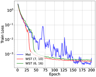
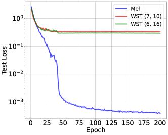
Figure 7: Loss per epoch during training. Left plot: training loss, which appears more stable when utilizing WST. Right plot: loss computed on test set. Similar to the training loss, the use of WST seems to enhance stability its stability, but employing the Mel spectrogram enables the model to reach a smaller value.

	Accuracy	Weighted F1-score	F1-score	AUC
AVES-bio (Hagiwara, 2023)	0.879	-	-	-
ResNet (Murphy et al., 2022)	-	-	0.867	0.928
Transfer Learning (Ghani et al., 2023)	0.83	-	-	0.98
BEANS (Hagiwara et al., 2023)	0.870	-	-	-
WST + our model Figure 4	0.94	0.94	0.90	0.996
Mel spectrogram + our model Figure 4	0.96	0.96	0.92	0.998

Table 1: Main Results. Considering the classification task on the entire WMMD dataset (Sayigh et al., 2016), we compare state-of-the-art benchmarks with our proposal (last two rows). Optimal batch size was found to be $128$.We report, when available in case of existing results, standard performance metrics as the accuracy, the F1-score, and the AUC score, computed on the test set at the end of training. Since the number of elements per class varies significantly, we report the weighted F1-score too. The top performance for each metric is emphasized. Disclaimer: (Hagiwara et al., 2023), (Murphy et al., 2022), (Ghani et al., 2023) use just the ”best of” subset of the full dataset, cfr. (Sayigh et al., 2016), while we use the full dataset. In (Hagiwara, 2023) is not specified.

As far as the Mel spectrogram is concerned, we fixed the number of Mel frequencies at 64 to avoid undesired border effects. The hop length parameter was set to 200, resulting in a single-channel Mel spectrogram dimension of 41$\times$64 for each signal. Similar to the WST methodology, each spectrogram underwent normalization. We plot in Figure 1 examples of Mel spectrogram and WST of first and second order obtained after the described data preparation pipeline.

3.2 Classification

In this section, we provide a detailed description of the classification pipeline, including both the architectures and the training setup used. Finally, we will present the results in terms of accuracy, F1-score, and AUC score, highlighting the comparison with state-of-the-art benchmarks.
In Figure 4, we summarize the architecture employed in our study. Due to the dataset’s significant imbalance, we prepared test and training sets with stratification (see Figure 3). For each class, $25\%$ of examples were allocated to the test set, while $75\%$ were assigned to the training set. We utilized the cross-entropy loss and Adam optimizer with decoupled weight decay (Loshchilov & Hutter, 2018). The initial learning rate was set at $10^{-2}$, and weight decay regularization with a hyperparameter of $10^{-3}$ was applied. Additionally, a scheduler for learning rate reduction on a plateau was incorporated. In Figure 6, we plot the test and train accuracy during training for Mel spectrogram and for three choices of the couple $(J,Q)$, maintaining a fixed minibatch size of $128$. Similar plots for other choices of batch size are available in Appendix A.
Table 1 displays the quantitative performance of the trained models after $200$ epochs, compared with existing benchmarks. Due to the dataset’s significant class imbalance, we also compute a version of F1-score weighted with respect to the number of elements per class. Evidently, our pipeline outperforms state-of-the-art models by $6-8\%$, achieving $94\%$ and $96\%$ accuracy for WST and Mel spectrogram, respectively—exceeding the symbolic threshold of $90\%$. Despite appearing as a small absolute improvement, the percentage of misclassifications in benchmark models, around $12\%$, is more than halved in our proposal, which represent a notable improvement in solving a classification task on the dataset in study.

4 Conclusions

In this study, we focused on the Watkins Marine Mammal Sound Database (WMMD), a comprehensive and labeled dataset of marine mammal vocalizations. Due to its pronounced imbalance and heterogeneity in terms of signal length, data preparation, and classification tasks posed considerable challenges. In this paper, we initially introduced a clear and straightforward data preparation pipeline, employing a time-frequency analysis based on Mel spectrograms — a standard approach, in contrast to an alternative method based on Wavelet Scattering Transform (WST).
Subsequently, we addressed a classification task on the entire dataset utilizing a deep architecture with residual layers. Our approach surpassed state-of-the-art accuracy results by $8\%$ using Mel spectrograms and $6\%$, achieving accuracy values of $96\%$ of correct predictions. The reached accuracy is notable, especially considering the heterogeneity of the dataset, both in signal length and class distribution. Plus, existing works usually focused just on subsets of the full dataset. Given this performance, we conclude that the precision of our method can be of fundamental importance for bioacoustics, bridging the gap between the data science and biology communities.
Furthermore, the analyzed dataset itself serves as a crucial case study for machine learning applications to natural datasets. Building upon the presented results, future directions could involve a more thorough investigation of optimal parameter pairs $(J,Q)$ and other hyperparameters of the model. It would be possible to implement a majority voting routine that consider simultaneously two parallel networks trained on WST and Mel spectrogram. However, we believe that any further improvement in accuracy would necessitate better class balancing, potentially through additional measurements or data augmentation for the less-represented species in the dataset. With these adjustments, near-perfect classification could be within reach.

Impact Statement

This paper presents work whose goal is to advance the field of Machine Learning. There are many potential societal consequences of our work, none which we feel must be specifically highlighted here.

Appendix A Additional Experimental Results.

In this section we report some additional experimental results. In Figures 8 and 9 we show the loss and accuracy per epoch for batch sizes of $64$ and $256$ respectively. A choice of a smaller batch size makes the training less stable, while there is no particular difference from a choice of $128$, as presented in the main body, and $256$ in Figure 9. In Table 2 we report the summary of the performances for other tested combinations of hyperparameters.

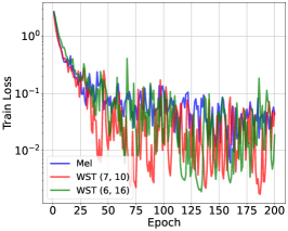
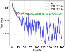
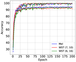
Figure 8: Metrics during training per epoch. Batch size of $64$. Left: loss on training set. Center: loss on test set. Right: accuracy on test set (solid line) and on training set (dashed line).

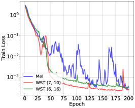
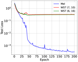
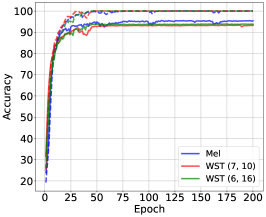
Figure 9: Metrics during training per epoch. Batch size of $256$. Left: loss on training set. Center: loss on test set. Right: accuracy on test set (solid line) and on training set (dashed line).

Representation	Batch Size	Accuracy	Weighted F1-score	F1-score	AUC
Mel	64	0.94	0.94	0.90	0.997
Mel	128	0.96	0.96	0.92	0.998
Mel	256	0.95	0.95	0.93	0.998
WST (6,16)	64	0.94	0.94	0.91	0.996
WST (6,16)	128	0.94	0.94	0.90	0.996
WST (6,16)	256	0.94	0.94	0.90	0.996
WST (7,10)	64	0.91	0.91	0.87	0.995
WST (7,10)	128	0.93	0.93	0.88	0.995
WST (7,10)	256	0.93	0.93	0.88	0.996

Table 2: Performance on validation set after training for different hyperparameters, namely $(J,Q)$ for the WST and batch size.

References

- Aghabozorgi et al. (2015) Aghabozorgi, S., Shirkhorshidi, A. S., and Wah, T. Y. Time-series clustering–a decade review. Information systems, 53:16–38, 2015.
- Andén & Mallat (2014) Andén, J. and Mallat, S. Deep scattering spectrum. IEEE Transactions on Signal Processing, 62(16):4114–4128, 2014.
- Andreux et al. (2020) Andreux, M., Angles, T., Exarchakis, G., Leonarduzzi, R., Rochette, G., Thiry, L., Zarka, J., Mallat, S., Andén, J., Belilovsky, E., et al. Kymatio: Scattering transforms in python. Journal of Machine Learning Research, 21(60):1–6, 2020.
- Bach et al. (2023) Bach, N. H., Vu, L. H., Nguyen, V. D., and Pham, D. P. Classifying marine mammals signal using cubic splines interpolation combining with triple loss variational auto-encoder. Scientific Reports, 13(1):19984, 2023.
- Bermant et al. (2019) Bermant, P. C., Bronstein, M. M., Wood, R. J., Gero, S., and Gruber, D. F. Deep machine learning techniques for the detection and classification of sperm whale bioacoustics. Scientific reports, 9(1):12588, 2019.
- Bruna (2013) Bruna, J. Scattering Representations for Recognition. Theses, Ecole Polytechnique X, February 2013. URL https://pastel.archives-ouvertes.fr/pastel-00905109. Déposée Novembre 2012.
- Bruna & Mallat (2013) Bruna, J. and Mallat, S. Invariant scattering convolution networks. IEEE transactions on pattern analysis and machine intelligence, 35(8):1872–1886, 2013.
- Bruna & Mallat (2019) Bruna, J. and Mallat, S. Multiscale sparse microcanonical models. Mathematical Statistics and Learning, 1(3):257–315, 2019.
- Cheng et al. (2020) Cheng, S., Ting, Y.-S., Ménard, B., and Bruna, J. A new approach to observational cosmology using the scattering transform. Monthly Notices of the Royal Astronomical Society, 499(4):5902–5914, 2020.
- Croll et al. (2001) Croll, D. A., Clark, C. W., Calambokidis, J., Ellison, W. T., and Tershy, B. R. Effect of anthropogenic low-frequency noise on the foraging ecology of balaenoptera whales. In Animal Conservation forum, volume 4, pp. 13–27. Cambridge University Press, 2001.
- Dudzinski et al. (2009) Dudzinski, K. M., Thomas, J. A., and Gregg, J. D. Communication in marine mammals. In Encyclopedia of marine mammals, pp. 260–269. Elsevier, 2009.
- Fu (2011) Fu, T.-c. A review on time series data mining. Engineering Applications of Artificial Intelligence, 24(1):164–181, 2011.
- Ghani et al. (2023) Ghani, B., Denton, T., Kahl, S., and Klinck, H. Global birdsong embeddings enable superior transfer learning for bioacoustic classification. Scientific Reports, 13(1):22876, 2023.
- Gibb et al. (2019) Gibb, R., Browning, E., Glover-Kapfer, P., and Jones, K. E. Emerging opportunities and challenges for passive acoustics in ecological assessment and monitoring. Methods in Ecology and Evolution, 10(2):169–185, 2019.
- Glinsky et al. (2020) Glinsky, M. E., Moore, T. W., Lewis, W. E., Weis, M. R., Jennings, C. A., Ampleford, D. J., Knapp, P. F., Harding, E. C., Gomez, M. R., and Harvey-Thompson, A. J. Quantification of maglif morphology using the mallat scattering transformation. Physics of Plasmas, 27(11), 2020.
- Hagiwara (2023) Hagiwara, M. Aves: Animal vocalization encoder based on self-supervision. In ICASSP 2023-2023 IEEE International Conference on Acoustics, Speech and Signal Processing (ICASSP), pp. 1–5. IEEE, 2023.
- Hagiwara et al. (2023) Hagiwara, M., Hoffman, B., Liu, J.-Y., Cusimano, M., Effenberger, F., and Zacarian, K. Beans: The benchmark of animal sounds. In ICASSP 2023-2023 IEEE International Conference on Acoustics, Speech and Signal Processing (ICASSP), pp. 1–5. IEEE, 2023.
- Khatami et al. (2018) Khatami, F., Wöhr, M., Read, H. L., and Escabí, M. A. Origins of scale invariance in vocalization sequences and speech. PLoS computational biology, 14(4):e1005996, 2018.
- Lee et al. (2006) Lee, C.-H., Chou, C.-H., Han, C.-C., and Huang, R.-Z. Automatic recognition of animal vocalizations using averaged mfcc and linear discriminant analysis. pattern recognition letters, 27(2):93–101, 2006.
- Loshchilov & Hutter (2018) Loshchilov, I. and Hutter, F. Decoupled weight decay regularization. In International Conference on Learning Representations, 2018.
- Lu et al. (2021) Lu, T., Han, B., and Yu, F. Detection and classification of marine mammal sounds using alexnet with transfer learning. Ecological Informatics, 62:101277, 2021.
- Macleod et al. (2021) Macleod, D. M., Areeda, J. S., Coughlin, S. B., Massinger, T. J., and Urban, A. L. GWpy: A Python package for gravitational-wave astrophysics. SoftwareX, 13:100657, 2021. ISSN 2352-7110. doi: 10.1016/j.softx.2021.100657. URL https://www.sciencedirect.com/science/article/pii/S2352711021000029.
- Mallat (1999) Mallat, S. A wavelet tour of signal processing. Elsevier, 1999.
- Mallat (2012) Mallat, S. Group invariant scattering. Communications on Pure and Applied Mathematics, 65(10):1331–1398, 2012.
- Marchand et al. (2022) Marchand, T., Ozawa, M., Biroli, G., and Mallat, S. Wavelet conditional renormalization group. arXiv preprint arXiv:2207.04941, 2022.
- Mazhar et al. (2007) Mazhar, S., Ura, T., and Bahl, R. Vocalization based individual classification of humpback whales using support vector machine. In OCEANS 2007, pp. 1–9. IEEE, 2007.
- Murphy et al. (2022) Murphy, D. T., Ioup, E., Hoque, M. T., and Abdelguerfi, M. Residual learning for marine mammal classification. IEEE Access, 10:118409–118418, 2022.
- Mustill (2022) Mustill, T. How to Speak Whale: The Power and Wonder of Listening to Animals. Hachette UK, 2022.
- Rabiner & Schafer (2010) Rabiner, L. and Schafer, R. Theory and applications of digital speech processing. Prentice Hall Press, 2010.
- Roberts & Mullis (1987) Roberts, R. A. and Mullis, C. T. Digital signal processing. Addison-Wesley Longman Publishing Co., Inc., 1987.
- Sayigh et al. (2016) Sayigh, L., Daher, M. A., Allen, J., Gordon, H., Joyce, K., Stuhlmann, C., and Tyack, P. The watkins marine mammal sound database: an online, freely accessible resource. In Proceedings of Meetings on Acoustics, volume 27. AIP Publishing, 2016.
- Valogiannis & Dvorkin (2022) Valogiannis, G. and Dvorkin, C. Towards an optimal estimation of cosmological parameters with the wavelet scattering transform. Physical Review D, 105(10):103534, 2022.
- Watkins & Wartzok (1985) Watkins, W. A. and Wartzok, D. Sensory biophysics of marine mammals. Marine Mammal Science, 1(3):219–260, 1985.