On an abrasion motivated fractal model

Abstract

In this paper, we consider a fractal model motivated by the abrasion of convex polyhedra, where the abrasion is realised by chipping small neighbourhoods of vertices. We study the upper box-counting dimension of the limiting object after infinitely many chipping.

1 Introduction

1.1 Motivation

Abrasion under collisions (also called collisional abrasion or chipping) is one of the main geological processes governing the evolution of natural shapes, ranging from pebbles to asteroids [7, 10, 23]. The process is driven by a sequence of discrete collisions where abraded particle collides with abraders. Based on their energy, collisions emerge in three well-separated phases [24]: large energy collisions belong to the fragmentation phase where cracks propagate through the entire particle, which is ultimately split into several parts of comparable volume. Medium energy collisions belong to the cleavage phase where the removed volume is smaller, but the crack propagates into the interior of the particle. Finally, in the abrasion phase (also called chipping phase), we consider small energy collisions where cracks remain in the vicinity of the surface and a small portion of the material is removed.

Geometric models of the high energy (fragmentation) phase and of the low energy (abrasion) phase have been studied in considerable detail. In the case of fragmentation, geometric models consider the bisection of convex polyhedra by random planes and study the combinatorial and metric properties of the descendant polyhedra [2, 8, 9]. In the case of abrasion, considering the limit where collision energy approaches zero led to the study of mean field geometric partial differential equations (PDEs) [3, 5, 15, 17], describing the evolution of shape as a function of continuous time. If one considers the original collision process associated with finite impact energies, then discrete time evolution models appear to be a natural choice [7, 24]. While no rigorous result is known that connects discrete-time models to PDE models, their predictions show very good qualitative match [7, 24], suggesting that the geometric study of discrete-time collision models may shed light on general features of shape evolution.

While the discreteness of shape evolution models referred so far only to time, in such models, convex polyhedra are the natural choice as geometric approximations of the studied particle. This choice is natural not only because (as we outline below) discrete time steps are best understood on discrete geometric objects but also because the 3D scanned images of particles on which computer codes can operate are also polyhedral objects [20].

The low energy, abrasion phase, geometric models of collisions are truncations of the polyhedral model, which remove small portions of its volume. If the latter is sufficiently small then, from the combinatorial point of view, we can distinguish between three kinds of local events where (a) one vertex is removed and one face is created, (b) one edge is removed and one face is created and (c) one face retreats parallel to itself and the combinatorial structure of the polyhedron remains invariant. These three local events do not differ from the point of view of collision energy. However, they differ from the point of view of the relative size and shape of the abraded particle with respect to the abrading particle [3, 6, 16]. In particular, event (a) corresponds to the case when the abrader is much larger, and event (c) to the case when the abrader is much smaller than the abraded particle. While none of these three events can, on its own, fully capture collisional shape evolution in the low energy (abrasion) phase, still, the individual study of these events can provide both geometric and physical insight. Moreover, in some cases, one single event reproduces global shape features with remarkable accuracy.

Our goal is the detailed geometric description of the event (a) when one vertex is removed in each step of the shape evolution process. Such discrete steps are called chipping events [22, 27]. In our paper, we will remove all vertices simultaneously, and we refer to this collective event as a single chipping event. The planar version of the chipping event was studied earlier in [27], revealing the emergence of fractal-like contours. Our goal is to offer a full and rigorous geometric study of this phenomenon in three dimensions. As noted above, event (a) corresponds to the case where the abrading object is much larger than the abraded particle, and this is a realistic approximation of pebbles carried in mountain rivers and evolving under collisions with the riverbed. Figure 1 shows an andesite rock that has been abraded in the Poprad River in the Tatra mountains. As a visual comparison, we show a polyhedron with 2912 faces, which was produced from a cube via six consecutive chipping events. Figure 2 shows the vicinity of one vertex of the cube as well as the Apollonian gasket for visual comparison.

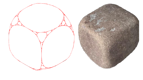
Figure 1: Left: Cube after six iterative chipping events with random orientation, having 2912 faces. Right: Moderately abraded andesite rock recovered from the Poprad river, at the foot of the High Tatra mountains.

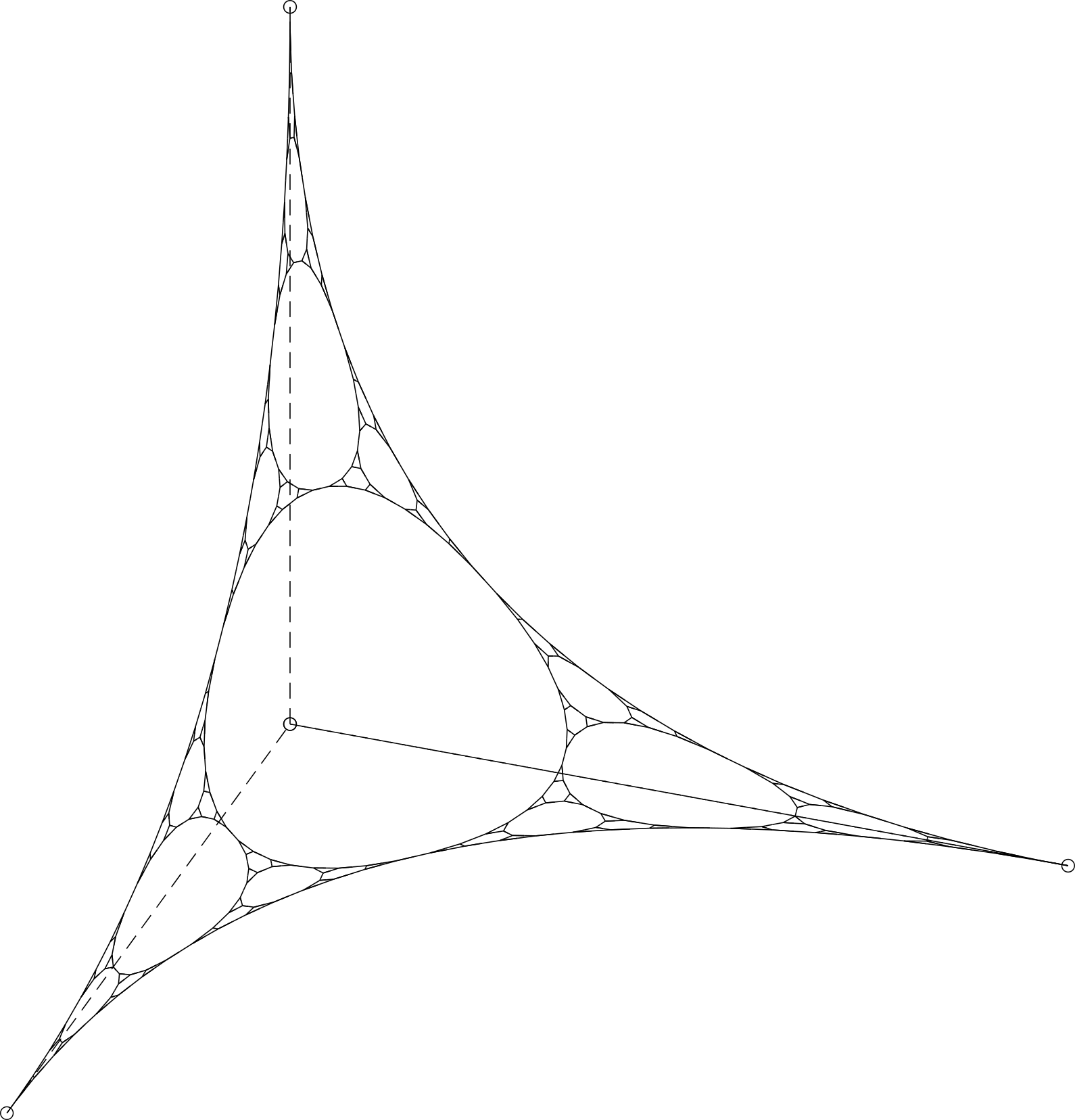
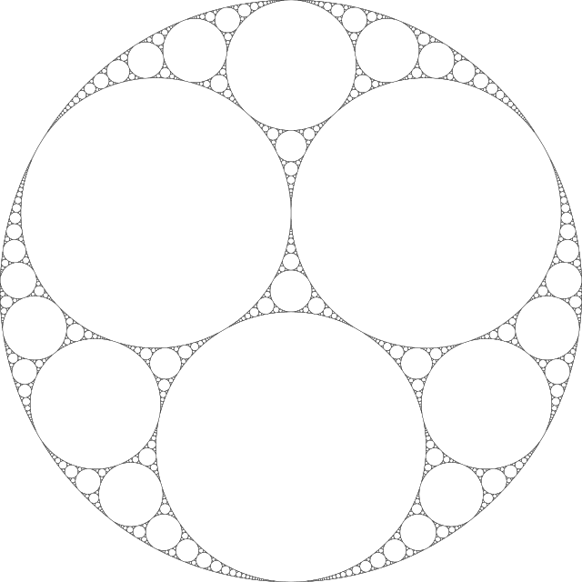
Figure 2: left: Figure of a simulation of chipping in the proximity of an original vertex of the initial polyhedron. right: the Apollonian gasket

Motivated by this visual analogy, we are interested in the geometric description of the limit where the number of chipping events approaches infinity. In this limit, the polyhedron (more precisely, its edge network) approaches a fractal-like object, and our main result (Theorem 1) determines the box-counting dimension of this object.

In fractal geometry, one of the cardinal questions is the dimension of the object under consideration. There are several different kinds of dimensions that are devoted to measuring how much the fractal set is spread. An advantage of the box-counting dimension is that there are available methods that allow us to study the dimension of actual 3D scanned images of particles, but unfortunately, these methods might give some relatively good approaches only at certain scales.

It turns out that our model is strongly connected to the so-called self-affine sets, which have been extensively studied in the last decades; see [1, 13, 14, 18, 19, 26]. The dimension theory of such objects is highly non-trivial. For instance, even in cases where a formula for the value of the dimension is known, it cannot be calculated explicitly, only implicitly, and it can be approximated well only in some cases; see [21, 25]. This is due to the extremely difficult structure of the group of matrix products.

In our case, this difficulty arises as well. Namely, we can give only an implicit formula for the box-counting dimension, which depends only on the chippings. That is, the value of the dimension is independent of the initial polyhedron.

The structure of the paper is as follows: In Section 2, we give a definition for chipping, and for further analysis, we introduce the local chart representation of simple convex polyhedra, and we define a sequence of iterated function systems (IFS) corresponding to the chipping. Finally, section 3 is devoted to the proof of Theorem 1.

2 The model, the iterated function scheme representation, and the dimension

2.1 The chipping model and the limit set

Let $P$ be a convex polyhedron, that is, let $\mathcal{V}$ be a finite subset of $\mathbb{R}^{3}$ and let $P=\mathrm{conv}(\mathcal{V})$ be the convex hull of $\mathcal{V}$ such that every point of $\mathcal{V}$ is an extremal point of $P$. We call $\mathcal{V}=\mathcal{V}(P)$ the set of vertices of $P$. Furthermore, let $\mathcal{E}=\mathcal{E}(P)$ be the set of edges. That is, for any two distinct $A,B\in\mathcal{V}$,

$$[A,B]=\{tA+(1-t)B:0\leq t\leq 1\}\in\mathcal{E}(P)$$

if and only if every $x\in[A,B]$ has a unique representation by the convex combination of vertices using only $A$ and $B$. Let $H$ be the net of edges, i.e. $H=H(P)=\bigcup_{[A,B]\in\mathcal{E}(P)}[A,B]$.

Let us index the vertices of $P$ by a finite set $I=I(P)$, i.e. $\mathcal{V}(P)=\{A_{i}:i\in I(P)\}$. For simpler notations, in some cases, we refer directly to members of $\mathcal{V}(P)$ by their indices. Let $E(P)\subseteq I(P)\times I(P)$ be such that $(i,j)\in E(P)$ if and only if $[A_{i},A_{j}]\in\mathcal{E}(P)$. We use the convention that $E(P)$ is symmetric, i.e., $(i,j)\in E(P)$ if and only if $(j,i)\in E(P)$. For a $j\in I$, let $N(j)$ be the set vertices which are the neighbours of $j$, that is, $i\in N(j)$ if and only if $(j,i)\in E(I)$. We call the convex polyhedron $P$ simple if $\#N(j)=3$ for every $j\in I(P)$. Furthermore, let $\mathcal{F}(P)$ be the set of faces of the polyhedron $P$, and for an $S\in\mathcal{F}(P)$, denote by $\mathbf{n}(S)$ a unit normal vector perpendicular to $S$. Finally, for a $j\in I$, let $M(j)$ be the set of faces $S$ such that $A_{j}$ is a vertex of $S$.

Now, we will define the way how a convex polyhedron evolves under the chipping algorithm. Let $j\in I(P)$ and let $\mathbf{n}_{j}$ be a vector such that $A_{j}+\varepsilon\mathbf{n}_{j}$ is an interior point of $P$ for every sufficiently small $\varepsilon>0$, and $\mathbf{n}_{j}$ is not parallel with any $\mathbf{n}(S)$ for every $S\in M(j)$. Let $\Psi_{j}$ be the hyperplane with normal vector $\mathbf{n}_{j}$, going through the point $A_{j}+\varepsilon_{j}\mathbf{n}_{j}$, and let $\Phi_{j}$ be the closed half-space determined by $\Psi_{j}$ such that $A_{j}$ is an interior point of $\Phi_{j}$, where $\varepsilon_{j}$ are chosen such that $(P\cap\Phi_{j})\cap(P\cap\Phi_{k})=\emptyset$ for every $j\neq k\in I(P)$. By chipping, we mean the removal of such $P\cap\Phi_{j}$ pyramids from all vertices of $P$, and the new chipped polyhedron is $\overline{\bigcup_{i\in I(P)}P\setminus\Phi_{i}}$.
By simple geometric arguments, it is easy to see that the chipping of vertices generates a simple polyhedron. Thus, from now on, we will always assume without loss of the generality that $P$ is simple. Furthermore, for the chipping of simple polyhedra, we can give the following simpler definition:

Definition 1 (chipping).

Let $P$ be a simple convex polyhedron with vertices $\mathcal{V}(P)$ indexed by $I$ and edges $\mathcal{E}(P)$ indexed by $E(P)\subseteq I(P)\times I(P)$. Let $\underline{p}=(p_{ij})_{(i,j)\in E(P)}$ be a vector of positive reals such that for every $i,j\in I(P)$ with $(i,j)\in E(I)$, $p_{ij}\in(0,1)$ and $p_{ij}+p_{ji}<1$. Let us call the vector $\underline{p}$ the chipping rate vector. We define the chipped polyhedron $\mathcal{C}_{\underline{p}}(P)$ as follows: let the set of vertices

$$\mathcal{V}(\mathcal{C}_{\underline{p}}(P)):=\{A_{j}+p_{ji}\overrightarrow{A_{j}A_{i}}:i,j\in I(P)\text{ such that }(i,j)\in E(P)\},$$

and $\mathcal{C}_{\underline{p}}(P)=\mathrm{conv}(\mathcal{V}(\mathcal{C}_{\underline{p}}(P)))$.

Let us index the vertices of $\mathcal{C}_{\underline{p}}(P)$ by $E(P)$, that is, let $I(\mathcal{C}_{\underline{p}}(P))=E(P)$ and $A_{ji}:=A_{j}+p_{ji}\overrightarrow{A_{j}A_{i}}$.

During the shape evolution of a simple polyhedron $P$ when one of its vertices $A_{j}$, which was in connection with $A_{i},A_{k}$ and $A_{l}$, is chipped, it is replaced by a new face composed of three new vertices which are named after the vertices they are created between $A_{ji},A_{jl}$ and $A_{jk}$. The vertex closer is noted first. chipping planes can only intersect edges starting from the chipped vertex. The new vertices are placed on the edges according to proportion $p_{ji},p_{jl},\text{ and }p_{jk}$. Similarly chipping $A_{ji}$ creates the new vertices $A_{jiij},A_{jijk},A_{jijl}$ dividing the edges according to $p_{jiij},p_{jijl}$, and $p_{jijk}$ etc. Moreover, it is easy to see that any $A_{ji},A_{kl}\in\mathcal{V}(\mathcal{C}_{\underline{p}}(P))$, $[A_{ji},A_{kl}]\in\mathcal{E}(\mathcal{C}_{\underline{p}}(P))$ if and only if $j=k$ or $j=l$ and $i=k$.

Let $j\in I(\mathcal{C}_{\underline{p}}(P))$. There exist unique $j^{\prime}\in I(P)$ and unique $i^{\prime}\in N(j^{\prime})$ such that $j=j^{\prime}i^{\prime}$. We call $j^{\prime}$ the mother of $j$, and we call $i^{\prime}$ the father of $j$. Furthermore, If $P$ is simple then $k\in N(j)$ if and only if $k=i^{\prime}j^{\prime}$ or there exists $i^{\prime}\neq k^{\prime}\in N(j^{\prime})$ such that $k=j^{\prime}k^{\prime}$. We call the vertex $i^{\prime}j^{\prime}\in N(j^{\prime}i^{\prime})$ the sibling of $j=j^{\prime}i^{\prime}$. Further, we call the vertices $j^{\prime}k^{\prime},j^{\prime}l^{\prime}\in N(j^{\prime}i^{\prime})$, where $k^{\prime},l^{\prime}\in N(j^{\prime})$ for $k^{\prime}\neq i^{\prime}$ and $l^{\prime}\neq i^{\prime}$, the cousins of $j^{\prime}i^{\prime}$. Let us denote the index of the sibling of $j$ by $s(j)$. For a visual representation of the chipping in a neighbourhood of a vertex, and for the family relations, see Figure 3.

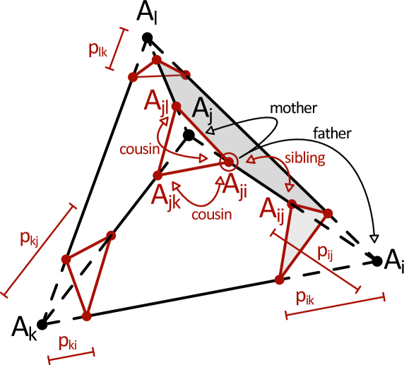
Figure 3: Chipping of a tetrahedron. Black color refers to the initial tetrahedron $P_{0}$, and red refers to the effect of chipping and chipping rates. Arrows show to the familiar relations of $A_{ji}$.

Note that the advantage of the described indexation is that there is a one-to-one correspondence between the indexes $E(P)$ of edges of $P$ and the vertices $I(\mathcal{C}_{\underline{p}}(P))$ of $\mathcal{C}_{\underline{p}}(P)$ since $E(P)$ is symmetric. In particular, $I(\mathcal{C}_{\underline{p}}(P))=E(P)$.

Using the chipping algorithm of Definition 1, we can define a sequence of simple convex polyhedra $P_{n}$ as follows: For any initial convex polyhedra $P_{0}=P$, let $\underline{p}_{0}$ be a chipping rate as in Definition 1, and let $P_{1}=\mathcal{C}_{\underline{p}_{0}}(P_{0})$. Suppose that the simple convex polyhedron $P_{n}$ is defined, then let $\underline{p}_{n}$ be a chipping rate on $E(P_{n})$ and let $P_{n+1}=\mathcal{C}_{\underline{p}_{n}}(P_{n})$. We call the sequence $P_{n}$ of polyhedra as chipping sequence.

Remark 1.

Note that as $n$ increases by one, the words describing the elements of $I(P_{n})$ are going to be $2^{n}$ long combinations of the indices of $I(P_{0})$. Words describing elements of $E(P_{n})$ are twice as long words.

The main object of our study is the limit set of the net of edges $H(P_{n})$ of the chipping sequence $P_{n}$. As we will see, there exists a unique compact set $X$ to which the sequence $H(P_{n})$ is converging in some proper sense (Hausdorff metric), and this set shows fractal-like properties strongly related to self-affine sets. For a discussion of this phenomenon, see Section 2.6.

Let us now define the Hausdorff metric of compact subsets of $\mathbb{R}^{3}$. For a set $X$ and $\delta>0$, let

$$[X]_{\delta}=\{y\in\mathbb{R}^{3}:\text{ there exists }x\in X\text{ such that }\|x-y\|<\delta\},$$

where $\|.\|$ denotes the usual Euclidean norm. We define the Hausdorff metric between two compact sets $X,Y\subset\mathbb{R}^{3}$

$$d_{H}(X,Y)=\inf\{\delta>0:Y\subset[X]_{\delta}\text{ and }X\subset[Y]_{\delta}\}.$$

It is well known that the set of compact subsets of $\mathbb{R}^{3}$ endowed with $d_{H}$ forms a complete metric space, see [12, Theorem 3.16]. It is easy to see that $d_{H}(\bigcup_{i=1}^{n}X_{i},\bigcup_{i=1}^{n}Y_{i})\leq\max_{i=1,\ldots,n}d_{H}(X_{i},Y_{i})$ and for any Lipschitz map $f$ with Lipschitz constant $C>0$, $d_{H}(f(X),f(Y))\leq Cd_{H}(X,Y)$.

Proposition 1.

Let $P_{n}$ be a chipping sequence such that there exists a $\delta>0$ such that for every $n\geq 1$ and $i\in I(P_{n})$, $\delta<p_{i}$ and for every $j\in N(i)$, $p_{i}+p_{j}<1-\delta$. Then there exists a unique compact set $X$ such that $d_{H}(H(P_{n}),X)\to 0$ as $n\to\infty$, where $H(P)$ is the net of edges of $P$.

We will give the proof of Proposition 1 later at the end of Section 2.5. In Figure 1, one can see the comparison of some realisations of the limit set of the chipping sequence and an abraded andesite rock found in Poprad River.

For short, we say that the chipping rates $\boldsymbol{p}=(\underline{p})_{n=1}^{\infty}$ are regular if there exists a $\delta>0$ such that for every $n\geq 1$ and $i\in I(P_{n})$, $\delta<p_{i}$ and for every $j\in N(i)$, $p_{i}+p_{j}<1-\delta$. The regularity of the chipping sequence roughly means that there is some fixed percentage such that at least that percentage of every edge is chipped in a neighbourhood of a vertex, but also a fixed percentage of every edge is kept.

2.2 Local representation of simple convex polyhedra

Let $P$ be a simple convex polyhedron. Now, we define a local representation of the edge net $H(P)$ of $P$ by affine mappings. Let us denote the usual orthogonal basis of $\mathbb{R}^{3}$ by $\{e_{1},e_{2},e_{3}\}$. Let $L=\bigcup_{i=1}^{3}[0,e_{i}]$.

Definition 2 (Local chart).

Let $P$ be an arbitrary, simple, convex polyhedron. Let $\boldsymbol{\lambda}=(\lambda_{ij})_{(i,j)\in E(P)}$ be a vector of positive reals such that for every $i,j\in I(P)$ with $(i,j)\in E(I)$, $\lambda_{ij}\in(0,1)$ and $\lambda_{ij}+\lambda_{ji}=1$.

Furthermore, for every $j\in I(P)$, let $\sigma_{j}\colon\{1,2,3\}\to N(j)$ be a permutation of the neighbourhood of $j$ and let $\sigma=(\sigma_{j})_{j\in I(P)}$. Let us define the matrix

$$\Lambda_{j,\sigma,\boldsymbol{\lambda}}.=\begin{bmatrix}\lambda_{j\sigma_{j}(1)}&0&0\\ 0&\lambda_{j\sigma_{j}(2)}&0\\ 0&0&\lambda_{j\sigma_{j}(3)}\end{bmatrix}.$$ (1)

Let $F_{j,\sigma,\boldsymbol{\lambda}}\colon\mathbb{R}^{3}\mapsto\mathbb{R}^{3}$ be such that

$$F_{j,\sigma,\boldsymbol{\lambda}}(x)=\begin{bmatrix}\overrightarrow{A_{j}A_{\sigma_{j}(1)}}&\overrightarrow{A_{j}A_{\sigma_{j}(2)}}&\overrightarrow{A_{j}A_{\sigma_{j}(3)}}\end{bmatrix}\Lambda_{j,\sigma,\boldsymbol{\lambda}}x+A_{j},$$

where $\overrightarrow{AB}$ denotes the vector with initial $A$ and endpoint $B$. We call $F_{j,\sigma,\boldsymbol{\lambda}}$ the local chart map of $j$ with permutation $\sigma$ and rate $\boldsymbol{\lambda}$, and we call $F_{j,\sigma,\boldsymbol{\lambda}}(L)$ the local neighbourhood of $j\in I(P)$.

For short, let $\boldsymbol{A}_{j,\sigma}:=\begin{bmatrix}\overrightarrow{A_{j}A_{\sigma_{j}(1)}}&\overrightarrow{A_{j}A_{\sigma_{j}(2)}}&\overrightarrow{A_{j}A_{\sigma_{j}(3)}}\end{bmatrix}$. By definition, $F_{j,\sigma,\boldsymbol{\lambda}}(0)=A_{j}$ and $F_{j,\sigma,\boldsymbol{\lambda}}(\underline{e}_{\ell})=\lambda_{j\sigma(\ell)}\cdot\overrightarrow{A_{j}A_{\sigma(\ell)}}+A_{j}$ for any $\ell=1,2,3$. Hence, $H(P)=\bigcup_{j\in I(P)}F_{j,\sigma,\boldsymbol{\lambda}}(L)$. Furthermore, we call the set of functions $\mathcal{F}_{\sigma,\boldsymbol{\lambda}}=\{F_{j,\sigma,\boldsymbol{\lambda}}\}_{j\in I(P)}$ as the chart of $H(P)$ with respect to the permutations $\sigma$ and rate $\boldsymbol{\lambda}$. For a visual representation of the local charts, see Figure 4.

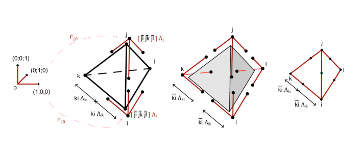
Figure 4: Cover of $H(P)$ by neighbourhoods.

2.3 Adapted charts

Let $P$ be a simple convex polyhedron and let $\{F_{j,\sigma,\boldsymbol{\lambda}}\}_{j\in I(P)}$ be a chart of $H(P)$ with permutations $\sigma=(\sigma_{j})_{j\in I(P)}$ and rates $\boldsymbol{\lambda}=(\lambda_{ij})_{(i,j)\in E(P)}$. We can use a chart effectively during the procedure of chipping if the closest cutting points on the edges of a vertex belong to the neighbourhood of the vertex. In the following, we will define how the chart of $P$ adapted to the chipping $\mathcal{C}_{\underline{p}}(P)$ in such a way.

Definition 3 (Adapted charts).

Let $P$ be a simple convex polyhedron, and let $\underline{p}=(p_{ij})_{(i,j)\in E(P)}$ be a chipping rate. Let $\mathcal{F}_{\sigma^{\prime},\boldsymbol{\lambda}^{\prime}}^{\prime}=\{F_{j^{\prime},\sigma^{\prime},\boldsymbol{\lambda}^{\prime}}\}_{j^{\prime}\in I(P)}$ be a chart of $H(P)$, and let $\mathcal{F}_{\sigma,\boldsymbol{\lambda}}=\{F_{j,\sigma,\boldsymbol{\lambda}}\}_{j\in I(\mathcal{C}_{\underline{p}}(P))}$ be a chart of $H(\mathcal{C}_{\underline{p}}(P))$.

We say that the chart $\mathcal{F}_{\sigma,\boldsymbol{\lambda}}$ is adapted to $\mathcal{F}_{\sigma^{\prime},\boldsymbol{\lambda}^{\prime}}^{\prime}$ if for every $j\in I(\mathcal{C}_{\underline{p}}(P))$ with mother $j^{\prime}\in I(P)$ with and father $i^{\prime}\in I(P)$ such that $N(j^{\prime})=\{i^{\prime},k^{\prime},l^{\prime}\}$, we have that $N(j)=\{i^{\prime}j^{\prime},j^{\prime}k^{\prime},j^{\prime}l^{\prime}\}$ and $\sigma_{j}((\sigma_{j^{\prime}}^{\prime})^{-1})(i^{\prime})=i^{\prime}j^{\prime}$, $\sigma_{j}((\sigma_{j^{\prime}}^{\prime})^{-1})(k^{\prime})=j^{\prime}k^{\prime}$ and $\sigma_{j}((\sigma_{j^{\prime}}^{\prime})^{-1})(l^{\prime})=j^{\prime}l^{\prime}$, moreover,

$$\Lambda_{j^{\prime},\sigma^{\prime},\boldsymbol{\lambda}^{\prime}}=\begin{bmatrix}p_{j^{\prime}\sigma^{\prime}_{j^{\prime}}(1)}&0&0\\ 0&p_{j^{\prime}\sigma^{\prime}_{j^{\prime}}(2)}&0\\ 0&0&p_{j^{\prime}\sigma^{\prime}_{j^{\prime}}(3)}\end{bmatrix}+\\ \begin{bmatrix}1-p_{\sigma^{\prime}_{j^{\prime}}(1)j^{\prime}}-p_{j^{\prime}\sigma^{\prime}_{j^{\prime}}(1)}&0&0\\ 0&1-p_{\sigma^{\prime}_{j^{\prime}}(2)j^{\prime}}-p_{j^{\prime}\sigma^{\prime}_{j^{\prime}}(2)}&0\\ 0&0&1-p_{\sigma^{\prime}_{j^{\prime}}(3)j^{\prime}}-p_{j^{\prime}\sigma^{\prime}_{j^{\prime}}(3)}\end{bmatrix}\Lambda_{j,\sigma,\boldsymbol{\lambda}}.$$

In particular, $\sigma$ being adapted to $\sigma^{\prime}$ means that $\sigma$ gives the same position to the neighbours of $j$ as the permutation $\sigma^{\prime}$ of the mother vertex of $j$ to the father vertices. Clearly, if the chart is adapted to the chipping, then for every $i,j\in I(P)$ with $(i,j)\in E(P)$, $p_{ij}<\lambda_{ij}$.

For a simple convex polyhedron $P$ and for $j,i\in I(P)$ with $(i,j)\in E(P)$, let us define a sibling sequence with respect to a chipping sequence $P_{n}=\mathcal{C}_{\underline{p}_{n}}(P_{n-1})$ with $P_{0}=P$ and chipping rates $\underline{p}=(p_{ij})_{(i,j)\in E(P_{n})}$ as follows: let $j_{0}=j$ and $i_{0}=i$. By induction, if $j_{n},i_{n}\in I(P_{n})$ such that $(i_{n},j_{n})\in E(P_{n})$ is defined then let $j_{n+1}=j_{n}i_{n}\in I(P_{n+1})$ and $i_{n+1}=i_{n}j_{n}\in I(P_{n+1})$, and by the definition of the chipping, $(i_{n+1},j_{n+1})\in E(P_{n+1})$. Clearly, the sibling of $j_{n}$ is $s(j_{n})=i_{n}$ for every $n\geq 1$. For the first two steps of the sibling sequence and the length of the edge between them, see Figure 5.

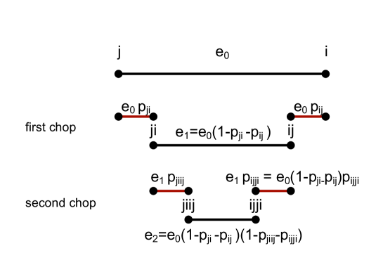
Figure 5: Effect of chipping on one edge

Lemma 1.

Let $P$ be a simple convex polyhedron, and let $P_{n}=\mathcal{C}_{\underline{p}_{n}}(P_{n-1})$ be a chipping sequence with $P_{0}=P$ and chipping rates $\underline{p}_{n}=(p_{ij})_{(i,j)\in E(P_{n-1})}$. Let $\mathcal{F}^{(n)}_{\sigma^{(n)},\boldsymbol{\lambda}^{(n)}}$ be charts of $H(P_{n})$ such that $\mathcal{F}^{(n)}_{\sigma^{(n)},\boldsymbol{\lambda}^{(n)}}$ is adapted to $\mathcal{F}^{(n-1)}_{\sigma^{(n-1)},\boldsymbol{\lambda}^{(n-1)}}$ for every $n\geq 1$. Then for every $j,i\in I(P)$ with $(i,j)\in E(P)$ we have

$$\lambda_{ji}=\sum_{k=1}^{\infty}p_{j_{k}}\prod_{\ell=1}^{k-1}(1-p_{j_{\ell}}-p_{s(j_{\ell})}),$$

where $j_{n}$ is the sibling sequence with initial vertices $j$ and $i$.

Proof.

By definition of adaptedness of charts,

$$\lambda_{ji}=p_{ji}+(1-p_{ji}-p_{ij})\lambda_{jiij}=p_{j_{1}}+(1-p_{j_{1}}-p_{s(j_{1})})\lambda_{j_{1}i_{1}}.$$

The proof can be finished now by induction. ∎

For a chipping sequence $P_{n}=\mathcal{C}_{\underline{p}_{n}}(P_{n-1})$, if $\mathcal{F}^{(n)}_{\sigma^{(n)},\boldsymbol{\lambda}^{(n)}}$ are charts of $H(P_{n})$ such that $\mathcal{F}^{(n)}_{\sigma^{(n)},\boldsymbol{\lambda}^{(n)}}$ is adapted to $\mathcal{F}^{(n-1)}_{\sigma^{(n-1)},\boldsymbol{\lambda}^{(n-1)}}$ for every $n\geq 1$ then we say that the sequence of charts is adapted. By the definition of adaptedness, $\sigma^{(0)}$ defines uniquely every permutation sequences $\sigma^{(n)}$ for every $n\geq 1$.

A simple corollary of Lemma 1 is that the chart $\mathcal{F}_{\sigma,\boldsymbol{\lambda}}$ of $H(P_{0})$ is uniquely determined by the chipping sequence $P_{n}=\mathcal{C}_{\underline{p}_{n}}(P_{n-1})$ and the vector of permutations $\sigma=(\sigma_{j})_{j\in I(P_{0})}$, and hence, it defines uniquely the sequence of adapted charts.

2.4 Construction of the iterated function systems

For a simple convex polyhedron $P$, chipping rates $\underline{p}=(p_{i^{\prime}j^{\prime}})_{(i^{\prime},j^{\prime})\in E(P)}$ and permutations $\sigma=(\sigma_{j})_{j\in I(\mathcal{C}_{\underline{p}}(P))}$, where $\sigma_{j}$ is a permutation of $N(j)$, let us define for every $j\in I(\mathcal{C}_{\underline{p}}(P))$ a $3\times 3$ matrix $C_{j,\sigma,\underline{p}}$ such that

$$C_{j,\sigma,\underline{p}}=\begin{cases}\begin{bmatrix}1-p_{j}-p_{\sigma(1)}&-p_{j}&-p_{j}\\ 0&p_{\sigma(2)}&0\\ 0&0&p_{\sigma(3)}\\ \end{bmatrix}&\text{if $\sigma(1)$ is the sibling of $j$,}\vspace{5pt}\\ \begin{bmatrix}p_{\sigma(1)}&0&0\\ -p_{j}&1-p_{\sigma(2)}-p_{j}&-p_{j}\\ 0&0&p_{\sigma(3)}\\ \end{bmatrix}&\text{if $\sigma(2)$ is the sibling of $j$, and}\vspace{5pt}\\ \begin{bmatrix}p_{\sigma(1)}&0&0\\ 0&p_{\sigma(2)}&0\\ -p_{j}&-p_{j}&1-p_{\sigma(3)}-p_{j}\\ \end{bmatrix}&\text{if $\sigma(3)$ is the sibling of $j$.}\end{cases}$$ (2)

Lemma 2.

Let $P$ be a simple convex polyhedron, and let $\underline{p}=(p_{ij})_{(i,j)\in E(P)}$ be a vector of chipping rates. Furthermore, let $\mathcal{F}_{\sigma,\boldsymbol{\lambda}}$ and $\mathcal{F}^{\prime}_{\sigma^{\prime},\boldsymbol{\lambda}^{\prime}}$ be charts of $H(\mathcal{C}_{\underline{p}}(P))$ and $H(P)$ respectively such that $\mathcal{F}_{\sigma,\boldsymbol{\lambda}}$ is adapted to $\mathcal{F}^{\prime}_{\sigma^{\prime},\boldsymbol{\lambda}^{\prime}}$.

Then for every $j\in I(\mathcal{C}_{\underline{p}}(P))$ with mother $j^{\prime}\in I(P)$ we have

$$F_{j,\sigma,\boldsymbol{\lambda}}=F_{j^{\prime},\sigma^{\prime},\boldsymbol{\lambda}^{\prime}}\circ G_{j^{\prime},j,\sigma^{\prime},\sigma,\underline{p}},$$

where $G_{j^{\prime},j,\sigma^{\prime},\sigma,\underline{p}}(x)=\Lambda_{j^{\prime},\sigma^{\prime},\boldsymbol{\lambda}^{\prime}}^{-1}\left(C_{j,\sigma,\underline{p}}\Lambda_{j,\sigma,\boldsymbol{\lambda}}x+p_{j}e_{\sigma^{-1}(s(j))}\right)$.

Proof.

Let $j\in I(\mathcal{C}_{\underline{p}}(P))$ be arbitrary. Let $j^{\prime}\in I(P)$ the mother, and $i^{\prime}\in N(j^{\prime})$ be the father of $j$, i.e. $j=j^{\prime}i^{\prime}$. Let us denote the other neighbours of $j^{\prime}$ by $N(j^{\prime})\setminus\{i^{\prime}\}=\{k^{\prime},l^{\prime}\}$. Then the neighbours of $j=j^{\prime}i^{\prime}$ are $i:=i^{\prime}j^{\prime}$, $k:=j^{\prime}k^{\prime}$ and $l:=j^{\prime}l^{\prime}$. In particular, $i^{\prime}j^{\prime}=s(j^{\prime}i^{\prime})=s(j)$. Hence,

$$A_{j} = A_{j^{\prime}i^{\prime}}=A_{j^{\prime}}+p_{j^{\prime}i^{\prime}}\overrightarrow{A_{j^{\prime}}A_{i^{\prime}}},$$

$$A_{i} = A_{i^{\prime}j^{\prime}}=A_{i^{\prime}}+p_{i^{\prime}j^{\prime}}\overrightarrow{A_{i^{\prime}}A_{j^{\prime}}},$$

$$A_{k} = A_{j^{\prime}k^{\prime}}=A_{j^{\prime}}+p_{j^{\prime}k^{\prime}}\overrightarrow{A_{j^{\prime}}A_{k^{\prime}}}\text{ and}$$

$$A_{l} = A_{j^{\prime}l^{\prime}}=A_{j^{\prime}}+p_{j^{\prime}l^{\prime}}\overrightarrow{A_{j^{\prime}}A_{l^{\prime}}}.$$

This implies that

$$\begin{split}\overrightarrow{A_{j}A_{i}}&=(1-p_{i^{\prime}j^{\prime}}-p_{j^{\prime}i^{\prime}})\overrightarrow{A_{j^{\prime}}A_{i^{\prime}}},\\ \overrightarrow{A_{j}A_{k}}&=p_{j^{\prime}k^{\prime}}\overrightarrow{A_{j^{\prime}}A_{k^{\prime}}}-p_{j^{\prime}i^{\prime}}\overrightarrow{A_{j^{\prime}}A_{i^{\prime}}},\\ \overrightarrow{A_{j}A_{l}}&=p_{j^{\prime}l^{\prime}}\overrightarrow{A_{j^{\prime}}A_{l^{\prime}}}-p_{j^{\prime}i^{\prime}}\overrightarrow{A_{j^{\prime}}A_{i^{\prime}}}.\end{split}$$ (3)

Thus, since the charts are adapted, we have $\sigma^{-1}_{j}(i)=\sigma^{-1}_{j^{\prime}}(i^{\prime})$, $\sigma^{-1}_{j}(k)=\sigma^{-1}_{j^{\prime}}(k^{\prime})$ and $\sigma^{-1}_{j}(l)=\sigma^{-1}_{j^{\prime}}(l^{\prime})$. So by (3) and the definition of matrix $C_{j,\sigma,\underline{p}}$ (2), we get

$$\boldsymbol{A}_{j,\sigma}=\boldsymbol{A}_{j^{\prime},\sigma^{\prime}}C_{j,\sigma,\underline{p}}.$$ (4)

Since $i=i^{\prime}j^{\prime}$ is the sibling of $j=j^{\prime}i^{\prime}$ we get by (4) that

$$\begin{split}F_{j,\sigma,\boldsymbol{\lambda}}(x)&=\boldsymbol{A}_{j,\sigma}\Lambda_{j,\sigma,\boldsymbol{\lambda}}x+A_{j}\\ &=\boldsymbol{A}_{j^{\prime},\sigma}C_{j,\sigma,\underline{p}}\Lambda_{j,\sigma,\boldsymbol{\lambda}}x+A_{j^{\prime}}+p_{j^{\prime}i^{\prime}}\overrightarrow{A_{j^{\prime}}A_{i^{\prime}}}\\ &=\boldsymbol{A}_{j^{\prime},\sigma}\left(C_{j,\sigma,\underline{p}}\Lambda_{j,\sigma,\boldsymbol{\lambda}}x+p_{j^{\prime}i^{\prime}}\underline{e}_{\sigma_{j^{\prime}}^{-1}(i^{\prime})}\right)+A_{j^{\prime}}\\ &=F_{j^{\prime},\sigma^{\prime},\boldsymbol{\lambda}^{\prime}}\left(\Lambda_{j^{\prime},\sigma^{\prime},\boldsymbol{\lambda}^{\prime}}^{-1}C_{j,\sigma,\underline{p}}\Lambda_{j,\sigma,\boldsymbol{\lambda}}x+p_{j^{\prime}i^{\prime}}\Lambda_{j^{\prime},\sigma^{\prime},\boldsymbol{\lambda}^{\prime}}^{-1}\underline{e}_{\sigma^{-1}_{j}(i)}\right),\end{split}$$

which had to be proven. ∎

Under the conditions of Lemma 2, the adaptedness of the charts (i.e. $\sigma^{-1}_{j}(i)=\sigma^{-1}_{j^{\prime}}(i^{\prime})$, $\sigma^{-1}_{j}(k)=\sigma^{-1}_{j^{\prime}}(k^{\prime})$ and $\sigma^{-1}_{j}(l)=\sigma^{-1}_{j^{\prime}}(l^{\prime})$) implies that

$$\begin{split}G_{j^{\prime},j,\sigma^{\prime},\sigma,\underline{p}}(\underline{e}_{\sigma^{-1}_{j}(s(j))})&=\underline{e}_{\sigma^{-1}_{j}(s(j))},\\ G_{j^{\prime},l,\sigma^{\prime},\sigma,\underline{p}}(\underline{e}_{\sigma_{j}^{-1}(k)})&=G_{j^{\prime},k,\sigma^{\prime},\sigma,\underline{p}}(\underline{e}_{\sigma_{j}^{-1}(l)})\text{ for }k\neq l\in N(j)\setminus\{s(j)\}.\end{split}$$ (5)

Hence,

$$G_{j^{\prime},j,\sigma^{\prime},\sigma,\underline{p}}(W)\subset W,$$ (6)

where $W$ is the tetrahedron defined by the vectors $\{0,e_{1},e_{2},e_{3}\}$.

2.5 Proof of the existence of the limiting object

Let now $P_{n}=\mathcal{C}_{\underline{p}_{n}}(P_{n-1})$ be a chipping sequence with $P_{0}=P$ and with chipping rates $\underline{p}_{n}=(p_{ij})_{(i,j)\in E(P_{n})}$. Let $\mathcal{F}^{(n)}_{\sigma^{(n)},\boldsymbol{\lambda}^{(n)}}$ be the uniquely determined sequence of adapted charts of $H(P_{n})$. For every $n\geq 1$ and $j_{n}\in I(P_{n})$, there exists a unique sequence $j_{k}\in I(P_{k})$ such that $j_{k}$ is the mother of $j_{k+1}$ for every $k=0,\ldots,n-1$. We call the sequence $\underline{j}=(j_{k})_{k=0}^{n-1}$ the mother sequence of $j_{n}$. Let us denote the set of infinite mother sequences by $\Sigma$ that is,

$$\Sigma=\{(j_{0},j_{1},\ldots):j_{k}\in I(P_{k})\text{ and }j_{k-1}\text{ is the mother of }j_{k}\}.$$

Furthermore, denote $\Sigma_{n}$, the set of mother sequences of length $n$ and denote $\Sigma_{*}$, the set of finite mother sequences. For a $\underline{j}\in\Sigma_{*}$, denote $|\underline{j}|$ the length of $\underline{j}$, that is, $|\underline{j}|=n$ for $\underline{j}=(j_{0},\ldots,j_{n})$.

By applying Lemma 2 inductively, we get

$$\begin{split}F_{j_{n},\sigma^{(n)},\boldsymbol{\lambda}^{(n)}}&=F_{j_{n-1},\sigma^{(n-1)},\boldsymbol{\lambda}^{(n-1)}}\circ G_{j_{n-1},j_{n},\sigma^{(n-1)},\sigma^{(n)},\underline{p}_{n}}\\ &=F_{j_{n},\sigma^{(0)},\boldsymbol{\lambda}^{(0)}}\circ G_{j_{0},j_{1},\sigma^{(0)},\sigma^{(1)},\underline{p}_{1}}\circ\cdots\circ G_{j_{n-1},j_{n},\sigma^{(n-1)},\sigma^{(n)},\underline{p}_{n}}.\end{split}$$ (7)

For a mother sequence $\underline{j}=(j_{0},\ldots,j_{n})$ and a sequence chipping rates $\boldsymbol{p}=(\underline{p}_{1},\ldots,\underline{p}_{n})$ let

$$G_{\underline{j},\sigma^{(0)},\boldsymbol{p}}:=G_{j_{0},j_{1},\sigma^{(0)},\sigma^{(1)},\underline{p}_{1}}\circ\cdots\circ G_{j_{n-1},j_{n},\sigma^{(n-1)},\sigma^{(n)},\underline{p}_{n}}.$$ (8)

Furthermore, let

$$C_{\underline{j},\sigma^{(0)},\boldsymbol{p}}:=C_{j_{1},\sigma^{(1)},\underline{p}_{1}}\cdots C_{j_{n},\sigma^{(n)},\underline{p}_{n}}.$$ (9)

Note that $\sigma^{(0)}$ determines uniquely the further permutations, so the product and composition above depend only on it. Moreover, for an integer $1\leq k\leq n-1$ let $\underline{j}|_{k}=(j_{1},\ldots,j_{k})$ and $\boldsymbol{p}|_{k}=(\underline{p}_{1},\ldots,\underline{p}_{k})$. For $k=0$, we use the conventions $\underline{j}|_{0}=\emptyset$, $\boldsymbol{p}|_{0}=\emptyset$, $C_{\emptyset,\emptyset}=\mathrm{Id}$.

It is easy to see by the definition of the map $G_{\underline{j},\sigma^{(0)},\boldsymbol{p}}$ that

$$G_{\underline{j},\sigma^{(0)},\boldsymbol{p}}(x)=\\ \Lambda_{j_{0},\sigma^{(0)},\boldsymbol{\lambda}^{(0)}}^{-1}\left(C_{\underline{j},\sigma^{(0)},\boldsymbol{p}}\ \Lambda_{j_{n},\sigma^{(n)},\boldsymbol{\lambda}^{(n)}}x+\sum_{k=1}^{n}p_{j_{k}}C_{\underline{j}|_{k-1},\sigma^{(0)},\boldsymbol{p}|_{k-1}}\underline{e}_{\sigma_{j_{k}}^{-1}(s(j_{k}))}\right).$$

Let us denote the set of indexes of vertices through the chipping by $I^{*}:=\bigcup_{n=0}^{\infty}I(P_{n})$.

Let us denote the singular values of a real $3\times 3$ matrix $A$ by $\alpha_{1}\geq\alpha_{2}\geq\alpha_{3}$. Clearly, for a $3\times 3$ matrix $A$, $\|A\|=\alpha_{1}(A)$, where $\|.\|$ is the induced norm by the usual Euclidean norm, and $\alpha_{3}(A)=\|A^{-1}\|^{-1}$. Furthermore, let $\|.\|_{1}$ be the $1$-norm of $\mathbb{R}^{3}$, that is, for $\underline{v}^{T}=(v_{1},v_{2},v_{3})\in\mathbb{R}^{3}$ $\|\underline{v}\|_{1}=|v_{1}|+|v_{2}|+|v_{3}|$. With a slight abuse of notation, let us denote the $1$-norm of $3\times 3$ matrices by $\|.\|_{1}$ too, that is, for a $3\times 3$ matrix $A=(a_{ij})_{i,j=1}^{3}$, we have $\|A\|_{1}=\max_{1\leq j\leq 3}\{|a_{1j}|+|a_{2j}|+|a_{3j}|\}$.

Lemma 3.

If the chipping rates $\boldsymbol{p}$ are regular then there exists $C>0$ such that for every $n\geq 1$ and every mother sequence $\underline{j}=(j_{0},\ldots,j_{n-1})$ of length $n$

$$\alpha_{1}(C_{\underline{j},\sigma^{(0)},\boldsymbol{p}})\leq C(1-\delta)^{n}.$$

Proof.

Since every two norms over finite dimensional vector spaces are equivalent, there exists $C>0$ such that

$$\alpha_{1}(C_{\underline{j},\sigma^{(0)},\boldsymbol{p}})\leq C\|C_{\underline{j},\sigma^{(0)},\boldsymbol{p}}\|_{1}\leq C\prod_{k=1}^{n}\|C_{j_{k},\sigma^{(0)},\underline{p}_{k}}\|_{1}.$$

On the other hand, for every matrix $C_{j,\sigma,\underline{p}}$ defined in (2)

$$\|C_{j,\sigma,\underline{p}}\|_{1}=\max\left\{1-p_{j}-p_{s(j)},\max_{k\in N(j)\setminus\{s(j)\}}\{p_{j}+p_{k}\}\right\}\leq 1-\delta,$$

which follows from the regularity of the rates. ∎

Now, we are ready to show the existence of the limit set of the sequence of net edges.

Proof of Proposition 1.

Let $P$ be a simple convex polyhedron. Let $\boldsymbol{p}=(\underline{p}_{n})_{n=1}^{\infty}$ be a sequence of regular chipping rates and let $P_{n}=\mathcal{C}_{\underline{p}_{n}}(P_{n-1})$ with $P_{0}=P$ be a chipping sequence.

Let us fix a permutation vector $\sigma^{(0)}=(\sigma_{j})_{j\in I(P)}$ and let $\mathcal{F}^{(n)}$ be a sequence of adapted charts of $H(P_{n})$. Note that $\boldsymbol{p}$ and $\sigma$ uniquely determine the sequence of adapted charts, so by a slight abuse of notation, we omit the fixed permutation from the notations.

Let $W$ be the tetrahedron defined by the vectors $\{\underline{0},\underline{e}_{1},\underline{e}_{2},\underline{e}_{3}\}$, and let $L=\bigcup_{i=1}^{3}[\underline{0},\underline{e}_{i}]$, where $[\underline{0},\underline{e}_{i}]=\{t\underline{e}_{i}:t\in[0,1]\}$. By definition, $H(P_{n})=\bigcup_{F\in\mathcal{F}^{(n)}}F(L)\subset\bigcup_{F\in\mathcal{F}^{(n)}}F(W)=:X_{n}$.

First, we show that $X_{n}$ converges to a limit set $X$ as $n\to\infty$. By Lemma 2 and (7), for every $F\in\mathcal{F}^{(n)}$ there exists a mother sequence $\underline{j}$ such that $F=F^{\prime}\circ G_{\underline{j}|_{n},\boldsymbol{p}|_{n}}$, where $F^{\prime}\in\mathcal{F}^{(0)}$. Thus, $X_{n}\subseteq X_{n-1}$ by (6). Clearly, $X_{n}$ are compact sets, and so there exists a non-empty compact set

$$X:=\bigcap_{n=1}^{\infty}X_{n}=\bigcap_{n=1}^{\infty}\bigcup_{F\in\mathcal{F}^{(n)}}F(W).$$ (10)

Furthermore, by Lemma 3,

$$\begin{split}&d_{H}(F^{\prime}\circ G_{\underline{j}|_{n-1},\boldsymbol{p}|_{n-1}}(W),F^{\prime}\circ G_{\underline{j}|_{n},\boldsymbol{p}|_{n}}(W))\\ &\qquad\leq\alpha_{1}(\boldsymbol{A}_{j_{0}}C_{\underline{j}|_{n-1},\boldsymbol{p}|_{n-1}}\Lambda_{j_{n-1},\boldsymbol{\lambda}^{(n-1)}})d_{H}(W,G_{j_{n-1},j_{n},\underline{p}_{n}}(W))\\ &\qquad\leq\alpha_{1}(\boldsymbol{A}_{j_{0}})C(1-\delta)^{n-1}\mathrm{diam}(W),\end{split}$$

where recall that $\boldsymbol{A}_{j_{0}}=\begin{bmatrix}\overrightarrow{A_{j_{0}}A_{\sigma_{j_{0}}(1)}}&\overrightarrow{A_{j_{0}}A_{\sigma_{j_{0}}(2)}}&\overrightarrow{A_{j_{0}}A_{\sigma_{j_{0}}(3)}}\end{bmatrix}$, and so

$$d_{H}(X_{n-1},X_{n})\leq(1-\delta)^{n-1}C\mathrm{diam}(W)\max_{j\in I(P)}\alpha_{1}(\boldsymbol{A}_{j}).$$

This implies that $X_{n}$ forms a Cauchy sequence, and so $X_{n}\to X$ in Hausdorff metric. Finally,

$$\begin{split}d_{H}(H(P_{n}),X_{n})&\leq\max_{F\in\mathcal{F}^{(n)}}d_{H}(F(L),F(W))\leq\max_{F\in\mathcal{F}^{(n)}}\mathrm{diam}(F(W))\\ &\leq\max_{j\in I(P)}\alpha_{1}(\boldsymbol{A}_{j})C(1-\delta)^{n-1}\mathrm{diam}(T),\end{split}$$

which completes the proof. ∎

2.6 The box-counting dimension

The main purpose of this paper is to study the fractal properties of the limit set $X$ defined in Proposition 1. There is no widely accepted definition of fractals. However, it is usually understood to be a set whose smaller parts resemble the whole. As we have seen by the construction (10) in Section 2.5, $X$ is a finite union of such sets since we repeat the same kind of chipping again and again. In particular, if the chipping rates $p_{ji}\equiv p$ were taken as a constant value independent of $n$ and $i,j\in I(P_{n})$, then the limiting object $X$ would be a finite union of so-called self-affine sets. More precisely, $X=\bigcup_{F^{\prime}\in\mathcal{F}^{(0)}}F^{\prime}(Y)$, where $Y$ is the unique non-empty compact set such that

$$Y=C_{1}Y+2pe_{1}\cup C_{2}Y+2pe_{2}\cup C_{3}Y+2pe_{3},$$

where $C_{i}$ is the matrix defined in (2) such that $j$ has sibling $\sigma(i)$.

Let us now define the box-counting dimension. Let $A$ be a bounded subset of $\mathbb{R}^{3}$. Let $N_{\delta}(A)$ be the minimal number of balls that cover $A$. We define the upper box-counting dimension as

$$\overline{\dim}_{B}(A)=\limsup_{\delta\to 0}\frac{\log N_{\delta}(A)}{-\log\delta}.$$

Two useful properties of the upper box-counting dimension are finite stability and monotonicity under Lipschitz mappings, that is, for every finite index set $J$

$$\overline{\dim}_{B}\left(\bigcup_{j\in J}A_{j}\right)=\max\{\overline{\dim}_{B}(A_{j}):j\in J\},$$

and for every map $f\colon\mathbb{R}^{3}\mapsto\mathbb{R}^{3}$ such that $\|f(\underline{x})-f(\underline{y})\|\leq L\|\underline{x}-\underline{y}\|$ for every $\underline{x},\underline{y}\in\mathbb{R}^{3}$ with some uniform constant $0<L$

$$\overline{\dim}_{B}\left(f(A)\right)\leq\overline{\dim}_{B}(A).$$

For further properties of the box-counting dimension, see [11, Section 3.1].

The difficulty which arises in the calculation of the dimension of self-affine-like objects is that they are defined by strict affine mappings. In other words, the most natural cover of $X$ is the collection $\{F(W)\}_{F\in\mathcal{F}^{(n)}}$ by the construction (10), but the sets $F(W)$ are relatively long and thin shapes which do not fit the required cover by balls. To handle this difficulty, let us define the singular value function introduced by Falconer [13]. For a $3\times 3$ matrix $A$, let

$$\varphi^{s}(A)=\begin{cases}\alpha_{1}(A)^{s}&\text{if }0\leq s\leq 1\\ \alpha_{1}(A)\alpha_{2}(A)^{s-1}&\text{if }1<s\leq 2\\ \alpha_{1}(A)\alpha_{2}(A)\alpha_{3}(A)^{s-2}&\text{if }2<s\leq 3\\ \big{(}\alpha_{1}(A)\alpha_{2}(A)\alpha_{3}(A)\big{)}^{s/3}&\text{if }s>3,\end{cases}$$

where $\alpha_{i}(A)$ denotes the $i$th singular value of $A$. The function $s\mapsto\varphi^{s}(A)$ is monotone decreasing, and the function $A\mapsto\varphi^{s}(A)$ is sub-multiplicative, i.e. for every $3\times 3$ matrices $A,B$, $\varphi^{s}(AB)\leq\varphi^{s}(A)\varphi^{s}(B)$ for every $s\geq 0$, see [13].

Theorem 1.

Let $P$ be a convex polyhedron, and let $P_{n}=\mathcal{C}_{\underline{p}_{n}}(P_{n-1})$ be a chipping sequence with $P_{0}=P$ and chipping rates $\underline{p}_{n}=(p_{i})_{i\in I(P_{n})}$. Let $\sigma^{(0)}$ be an arbitrary but fixed neighbourhood permutation of $P$. Furthermore, let $\{C_{\underline{j},\boldsymbol{p}}\}$ be the matrices defined in (2) and (9).

If there exists $\delta>0$ such that for every $j\in I^{*}=\bigcup_{n=0}^{\infty}I(P_{n})$ and $i\in N(j)$, $p_{j}>\delta$ and $p_{j}+p_{i}<1-\delta$ then

$$\overline{\dim}_{B}(X)=\inf\{s>0:\sum_{n=1}^{\infty}\sum_{\underline{j}\in\Sigma_{n}}\varphi^{s}(C_{\underline{j},\boldsymbol{p}|_{n}})<\infty\}.$$

Furthermore, $\overline{\dim}_{B}(X)\in[1,2]$.

The method of the proof uses the ideas of Falconer [14]. However, there are several technical difficulties; for instance, $X$ is not a planar, connected set.

3 The upper box dimension the edge net of the abraded polyhedron

We assume, without loss of generality, that $P_{0}$ is a simple convex polyhedron. Throughout the section we fix a $P_{n}=\mathcal{C}_{\underline{p}_{n}}(P_{n-1})$ chipping sequence with $P_{0}=P$ and chipping rates $\boldsymbol{p}=(\underline{p}_{n})_{n=1}^{\infty}$, where $\underline{p}_{n}=(p_{i})_{i\in I(P_{n})}=(p_{ij})_{(i,j)\in E(P_{n-1})}$, furthermore, we fix a neighbourhood permutation $\sigma=(\sigma_{j})_{j\in I(P)}$ of $P_{0}$. We will also assume throughout the section that chipping rates are regular, that is, there exists a $\delta>0$ such that for every $i\in I^{*}=\bigcup_{n=0}^{\infty}I(P_{n})$, $\delta<p_{i}$ and $p_{i}+p_{j}<1-\delta$ for every $j\in N(i)$.

To simplify the notations, we denote the adapted sequence of charts by $\mathcal{F}^{(n)}=\{F_{j}\}_{j\in I(P_{n})}$ and the matrix defined in (1) by $\Lambda_{j}$ for $j\in I^{*}$. Let us denote the matrices defined in (2) by $C_{j}$ for $j\in I^{*}$, and the matrices defined in (9) by $C_{\underline{j}}$ for mother sequences $\underline{j}\in\Sigma_{*}$. Similarly, for a $j\in I^{*}$ with mother $j^{\prime}$, let $G_{j^{\prime},j}$ be the map defined in Lemma 2 and for a mother sequence $\underline{j}\in\Sigma_{*}$, let $G_{\underline{j}}$ be defined in (8).

For a mother sequence $\underline{j}=(j_{0},j_{1},\ldots,j_{n})\in\Sigma_{n}$, let

$$B_{\underline{j}}:=\Lambda_{j_{0}}^{-1}C_{\underline{j}}\Lambda_{j_{n}}.$$

Simple algebraic calculations show that for every $j\in I^{*}$, the matrix $C_{j}^{-1}$ contains non-negative elements, hence, $(B_{\underline{j}})^{-1}$ has non-negative elements for every mother sequence $\underline{j}\in\Sigma_{*}$.

Let $s_{0}$ be as in Theorem 1. By Lemma 1 and the regularity of the chipping rates $\boldsymbol{p}$, we have that for every $j\in I^{*}$, $\delta<\lambda_{j}<1$, and so

$$s_{0}=\inf\{s>0:\sum_{\underline{j}\in\Sigma_{*}}\varphi^{s}(B_{\underline{j}})<\infty\}.$$ (11)

3.1 Singular values and separation

Before we prove the lower bound in Theorem 1, we need further analysis of the matrices $B_{\underline{j}}$. For an $\varepsilon\geq 0$, let us denote the triangle formed by the vertices $(1-2\varepsilon,\varepsilon,\varepsilon)$, $(\varepsilon,1-2\varepsilon,\varepsilon)$ and $(\varepsilon,\varepsilon,1-2\varepsilon)$ by $T_{\varepsilon}$. Let us denote the triangle formed by the vertices $\underline{e}_{1},\underline{e}_{2},\underline{e}_{3}$ by $T_{0}$. Let us denote the orthogonal projection to a proper subspace $Y$ of $\mathbb{R}^{3}$ by $\mathrm{proj}_{Y}$. Furthermore, let us denote the subspace perpendicular to $(1,1,1)$ by $V$ and for simplicity, by $\mathrm{proj}$ the orthogonal projection $\mathrm{proj}\colon\mathbb{R}^{3}\mapsto V$. Also, let us denote the standard scalar product on $\mathbb{R}^{3}$ by $\langle\cdot,\cdot\rangle$, and the angle between two vectors by $\sphericalangle(\cdot,\cdot)$.

Lemma 4.

For every $\varepsilon>0$, there exist a uniform constant $C>0$ such that for every $\underline{v}\in T_{\varepsilon}$, and every mother sequence $\underline{j}\in\Sigma_{*}$

$$\|(B_{\underline{j}})^{-1}\underline{v}\|\geq C\|(B_{\underline{j}})^{-1}\|.$$

Proof.

Let $A$ be an arbitrary but fixed matrix with strictly positive elements such that for every $\underline{w}\in T_{0}$, $A\underline{w}/\|A\underline{w}\|_{1}\in T_{\varepsilon}$. Since $(B_{\underline{j}})^{-1}\underline{v}$ has non-negative elements, we have $\frac{A(B_{\underline{j}})^{-1}\underline{v}}{\|A(B_{\underline{j}})^{-1}\underline{v}\|_{1}}\in T_{\varepsilon}$. By [4, Lemma 2.2], there exists a constant $C^{\prime}>0$ depending only on $\varepsilon>0$ such that

$$\|A(B_{\underline{j}})^{-1}\underline{v}\|\geq C^{\prime}\|A(B_{\underline{j}})^{-1}\|.$$

But clearly, $\|A(B_{\underline{j}})^{-1}\underline{v}\|\leq\|A\|\|(B_{\underline{j}})^{-1}\underline{v}\|$ and $\|A(B_{\underline{j}})^{-1}\|\geq\|A^{-1}\|^{-1}\|(B_{\underline{j}})^{-1}\|$, thus by choosing $C=C^{\prime}\|A^{-1}\|^{-1}\|A\|^{-1}$, the claim follows. ∎

An immediate corollary of Lemma 4 is that for every $\underline{v}\in T_{\varepsilon}$, every $n\geq 1$, every mother sequence $\underline{j}\in\Sigma_{*}$

$$\alpha_{3}(B_{\underline{j}})\geq C\|B_{\underline{j}}|(B_{\underline{j}})^{-1}V^{\perp}\|,$$ (12)

where $\|A|Y\|$ denotes the restricted norm of the $3\times 3$ matrix to the subspace $Y\subset\mathbb{R}^{3}$, that is, $\|A|Y\|=\sup_{\underline{v}\in Y}\|A\underline{v}\|$. More generally, denote by $\alpha_{i}(A|V)$ the $i$th singular value of the linear mapping $A|_{V}$ from $V$ to $\mathrm{Im}(A|_{V})$.

Lemma 5.

There exists $c>0$ such that for every mother sequence $\underline{j}\in\Sigma_{*}$ and for every $\underline{w}\in V$

$$\|\mathrm{proj}(B_{\underline{j}}\underline{w})\|\geq c\alpha_{2}(B_{\underline{j}})\|\underline{w}\|.$$

Proof.

Let $\underline{w}\in V$ be arbitrary. Then for any vector $\underline{v}\in V^{\perp}$

$$0=\langle\underline{w},\underline{v}\rangle=\left\langle B_{\underline{j}}\underline{w},\left((B_{\underline{j}})^{-1}\right)^{T}\underline{v}\right\rangle.$$

Since $\left((B_{\underline{j}})^{-1}\right)^{T}$ has non-negative elements, we have that $\left((B_{\underline{j}})^{-1}\right)^{T}\underline{v}$ is contained in the first octant $\{(x,y,z):x,y,z\geq 0\}$, and so there exists a positive $\delta>0$ such that $\sphericalangle(\underline{v},B_{\underline{j}}\underline{w})>\delta$ for every mother sequence $\underline{j}$ and every $\underline{w}\in V$. And so, there exists $c>0$ such that

$$\|\mathrm{proj}(B_{\underline{j}}\underline{w})\|\geq c\|B_{\underline{j}}\underline{w}\|.$$

Let $\underline{w}_{1},\underline{w_{2}}\in V$ be such that $\langle\underline{w}_{1},\underline{w}_{2}\rangle=0$, and let $Z$ be the parallelepiped formed by $\underline{w}_{1},\underline{w_{2}},(B_{\underline{j}})^{-1}\underline{v}$. Hence,

$$\begin{split}\alpha_{1}(B_{\underline{j}})\|\underline{w}_{1}\|\|B_{\underline{j}}\underline{w}_{2}\|\|\underline{v}\|&\geq\|B_{\underline{j}}\underline{w}_{1}\|\|B_{\underline{j}}\underline{w}_{2}\|\|\underline{v}\|\geq\mathrm{Vol}(B_{\underline{j}}(Z))\\ &=\alpha_{1}(B_{\underline{j}})\alpha_{2}(B_{\underline{j}})\alpha_{3}(B_{\underline{j}})\mathrm{Vol}(Z)\\ &\geq\alpha_{1}(B_{\underline{j}})\alpha_{2}(B_{\underline{j}})\alpha_{3}(B_{\underline{j}})\|\underline{w}_{1}\|\|\underline{w}_{2}\|\|(B_{\underline{j}})^{-1}\underline{v}\|\sqrt{2}/2\\ &\geq C\alpha_{1}(B_{\underline{j}})\alpha_{2}(B_{\underline{j}})\|\underline{w}_{1}\|\|\underline{w}_{2}\|,\end{split}$$

where in the last inequality, we used Lemma 4. Hence, the claim follows. ∎

Lemma 6.

For every mother sequence $\underline{j}\in\Sigma_{*}$ and every vector $\underline{w}$ with strictly positive coordinates, there exists $c>0$ such that

$$G_{\underline{j}}(\underline{0})+c\underline{w}\in G_{\underline{j}}(T_{0}).$$

In particular, for every $2$-dimensional subspace $Y$ with normal vector of strictly positive coordinates $\mathrm{proj}_{Y}(G_{\underline{j}}(W))=\mathrm{proj}_{Y}(G_{\underline{j}}(T_{0}))$.

Proof.

There exists $c\in\mathbb{R}$ such that $G_{\underline{j}}(\underline{0})+c\underline{w}$ is contained in the hyperplane $G_{\underline{j}}(V+\underline{v})$, where $\underline{v}=(1/3,1/3,1/3)$. Indeed, if not then $\underline{w}\in B_{\underline{j}}(V)$ and in particular, $(B_{\underline{j}})^{-1}\underline{w}\in V$. Since $(B_{\underline{j}})^{-1}\underline{w}$ has strictly positive coordinates this is impossible.

Now, let us argue by contradiction and suppose that$G_{\underline{j}}(\underline{0})+c\underline{w}\in G_{\underline{j}}(V+\underline{v})\setminus G_{\underline{j}}(T_{0})$. Clearly, $G_{\underline{j}}^{-1}(G_{\underline{j}}(\underline{0})+c\underline{w})=c(B_{\underline{j}})^{-1}\underline{w}\in(V+\underline{v})\setminus T_{0}$, but this is impossible since $(B_{\underline{j}})^{-1}\underline{w}$ has strictly positive elements.

Finally, let $Y\subset\mathbb{R}^{3}$ be a $2$-dimensional with normal vector $\underline{w}$. Since $\mathrm{proj}_{Y}(G_{\underline{j}}(\underline{0})+c\underline{w})=\mathrm{proj}_{Y}(G_{\underline{j}}(\underline{0}))$, the last claim follows. ∎

Lemma 7.

There exist a uniform constant $C>0$ such that for every mother sequence $\underline{j}\in\Sigma^{*}$

$$\mathrm{Area}\left(\mathrm{proj}(G_{\underline{j}}(T_{0}))\right)\geq C\alpha_{1}(B_{\underline{j}})\alpha_{2}(B_{\underline{j}}).$$

Proof.

Let $\underline{v}=(1/3,1/3,1/3)$ as usual. By Lemma 6, there exists $c>0$ such that $G_{\underline{j}}(\underline{0})+c\underline{v}\in G_{\underline{j}}(T_{0})$. Since $G_{\underline{j}}^{-1}(G_{\underline{j}}(\underline{0})+c\underline{v})=c(B_{\underline{j}})^{-1}\underline{v}\in T_{0}$, we have $\|c(B_{\underline{j}})^{-1}\underline{v}\|\leq 1$. Thus, by (12) we get

$$c\|\underline{v}\|=\left\|B_{\underline{j}}\frac{(B_{\underline{j}})^{-1}\underline{v}}{\|(B_{\underline{j}})^{-1}\underline{v}\|}\right\|\|c(B_{\underline{j}})^{-1}\underline{v}\|\leq C\alpha_{3}(B_{\underline{j}}).$$ (13)

Let us denote the height of $G_{\underline{j}}(W)$ with respect to the side $G_{\underline{j}}(T_{0})$ by $m$. Then

$$\begin{split}\alpha_{1}(B_{\underline{j}})\alpha_{2}(B_{\underline{j}})\alpha_{3}(B_{\underline{j}})\mathrm{Area(T_{0})}\frac{\sqrt{3}}{18}&=\alpha_{1}(B_{\underline{j}})\alpha_{2}(B_{\underline{j}})\alpha_{3}(B_{\underline{j}})\mathrm{Vol}(W)\\ &=\mathrm{Vol}(G_{\underline{j}}(W))=\mathrm{Area}(G_{\underline{j}}(T_{0}))m/6\\ &\leq\mathrm{Area}(G_{\underline{j}}(T_{0}))c\|\underline{v}\|/6\\ &\leq\mathrm{Area}(G_{\underline{j}}(T_{0}))\alpha_{3}(B_{\underline{j}})C/6,\end{split}$$

where in the last inequality we used (13). ∎

Lemma 8.

For every $n\geq 1$ and every mother sequences $\underline{j},\underline{j}^{\prime}\in\Sigma_{n}$ such that $j_{0}=j^{\prime}_{0}$ but $\underline{j}\neq\underline{j}^{\prime}$, i.e. there exists $1\leq k\leq n$ such that $j_{k}\neq j_{k}^{\prime}$ then

$$\mathrm{proj}(G_{\underline{j}}(W^{o}))\cap\mathrm{proj}(G_{\underline{j}^{\prime}}(W^{o}))=\emptyset,$$

where we recall that $\mathrm{proj}$ denotes the orthogonal projection to the subspace $V$ of normal vector $\underline{v}=(1/3,1/3,1/3)$.

Proof.

Let $1\leq k\leq n$ be the smallest integer such that $j_{k}\neq j_{k}^{\prime}$. Since $G_{i^{\prime},i}(W)\subseteq W$ for every $i\in I^{*}$ with mother $i^{\prime}$, it is enough to show that for every $2$-dimensional subspace $Y\subset\mathbb{R}^{2}$ with normal vector of strictly positive entries

$$\mathrm{proj}_{Y}(G_{j_{k-1},j_{k}}(W^{o}))\cap\mathrm{proj}_{Y}(G_{j_{k-1}^{\prime},j_{k}^{\prime}}(W^{o}))=\emptyset,$$

where $\mathrm{proj}_{Y}$ is the orthogonal projection to the subspace $Y$. Hence, by Lemma 6 it is enough to show that

$$\mathrm{proj}_{Y}(G_{j_{k-1},j_{k}}(T_{0}))^{o}\cap\mathrm{proj}_{Y}(G_{j_{k-1}^{\prime},j_{k}^{\prime}}(T_{0}))^{o}=\emptyset.$$

However, this follows by the fact that the common vertex of the triangles $G_{j_{k-1},j_{k}}(T_{0})$ and $G_{j_{k-1}^{\prime},j_{k}^{\prime}}(T_{0})$ is positioned on one of the same plane formed by coordinate axis and the other vertices are positioned on different coordinate-planes. ∎

Lemma 9.

There exists a constant $C>0$ such that for every mother sequence $\underline{j}\in\Sigma_{*}$ there exists an $i\in\{2,3\}$ such that

$$\|\operatorname{proj}(G_{\underline{j}}(\underline{e}_{i}))-\operatorname{proj}(G_{\underline{j}}(\underline{e}_{1}))\|\geq C\alpha_{1}(B_{\underline{j}}).$$

Proof.

Let us consider the singular value decomposition of the linear map $\operatorname{proj}B_{\underline{j}}|_{V}\colon V\mapsto V$. Namely, let $\underline{x}_{1},\underline{x}_{2}$ and $\underline{y}_{1},\underline{y}_{2}$ be orthonormal bases of $V$ such that $\operatorname{proj}B_{\underline{j}}\underline{x}_{i}=\alpha_{i}(\operatorname{proj}B_{\underline{j}}|V)\underline{y}_{i}$ for $i=1,2$.

Now, let us consider the exterior product $\bigwedge V$. Clearly, $\dim\bigwedge V=1$ and $\operatorname{proj}B_{\underline{j}}|_{V}$ induces a linear map $(\operatorname{proj}B_{\underline{j}}|_{V})^{\wedge}$ on $\bigwedge V$ naturally by

$$(\operatorname{proj}B_{\underline{j}}|_{V})^{\wedge}(\underline{x}\wedge\underline{y})=(\operatorname{proj}B_{\underline{j}}\underline{x})\wedge(\operatorname{proj}B_{\underline{j}}\underline{y})=:d_{\underline{j}}\ \underline{x}\wedge\underline{y},$$

where $d_{\underline{j}}=\alpha_{1}(\operatorname{proj}B_{\underline{j}}|V)\alpha_{2}(\operatorname{proj}B_{\underline{j}}|V)\in\mathbb{R}$. Since $\|\underline{x}\wedge\underline{y}\|$ is the area of the parallelogram formed by the vectors $\underline{x},\underline{y}\in V$, we get by Lemma 7 that there exists a constant $C>0$ such that for every mother sequence $\underline{j}\in\Sigma_{*}$

$$\alpha_{1}(\operatorname{proj}B_{\underline{j}}|V)\alpha_{2}(\operatorname{proj}B_{\underline{j}}|V)\geq C\alpha_{1}(B_{\underline{j}})\alpha_{2}(B_{\underline{j}}).$$ (14)

Furthermore, since $\alpha_{2}(B_{\underline{j}})\geq\inf_{\underline{w}\in V}\|\operatorname{proj}B_{\underline{j}}\underline{w}\|$ we have that

$$\alpha_{1}(\operatorname{proj}B_{\underline{j}}|V)\geq C\alpha_{1}(B_{\underline{j}}).$$ (15)

For every vector $\underline{z}\in V$ such that $\sphericalangle(\underline{x}_{1},\underline{z})<\pi/2-\varepsilon$, $\|\operatorname{proj}B_{\underline{j}}\underline{z}\|\geq\alpha_{1}(\operatorname{proj}B_{\underline{j}}|V)\|z\|\cos(\pi/2-\varepsilon)$. Since the angle between $\underline{e}_{3}-\underline{e}_{1}$ and $\underline{e}_{2}-\underline{e}_{1}$ is $\pi/3$, by choosing $\varepsilon=\pi/12$ we get that there is an $i\in\{2,3\}$ such that

$$\|\operatorname{proj}B_{\underline{j}}(\underline{e}_{i}-\underline{e}_{1})\|\geq\cos(5\pi/12)\|\underline{e}_{i}-\underline{e}_{1}\|\alpha_{1}(\operatorname{proj}B_{\underline{j}}|V).$$

The claim of the lemma follows from the combination of the previous inequality with (15). ∎

3.2 Upper bound

The proof of the upper bound is standard and follows easily from [14], but we give here the details for the convenience of the reader. First, we show that $s_{0}\leq 2$. The proof is similar to the proof of Lemma 11. However, it requires the more sophisticated estimates from Section 3.1.

Lemma 10.

Under the assumptions above, $s_{0}\leq 2$.

Proof.

By Lemma 6 and Lemma 8, for every $n\in\mathbb{N}$, $\bigcup\limits_{\underline{j}\in\Sigma_{n}}\mathrm{proj}\circ G_{\underline{j}}(T_{0})\subset T_{0}$ and $G_{\underline{j}}(T_{0})^{o}\cap G_{\underline{i}}(T_{0})^{o}=\emptyset$ for every $\underline{j}\neq\underline{i}\in\Sigma_{n}$. Hence, by Lemma 7

$$\begin{split}\mathrm{Area}(\mathrm{proj}(T_{0}))&\geq\sum_{\underline{j}\in\Sigma_{n}}\mathrm{Area}\left(\mathrm{proj}(G_{\underline{j}}(T_{0}))\right)\\ &\geq C\sum_{\underline{j}\in\Sigma_{n}}\alpha_{1}(B_{\underline{j}})\alpha_{2}(B_{\underline{j}}).\end{split}$$

On the other hand, by Lemma 1 and the regularity of the chipping rates $\boldsymbol{p}$, we have that for every $j\in I^{*}$, $\delta<\lambda_{j}<1$, and so by Lemma 3 there exists a constant $C>0$ such that for every $\underline{j}\in\Sigma_{*}$

$$\alpha_{3}(B_{\underline{j}})\leq\alpha_{1}(B_{\underline{j}})\leq C(1-\delta)^{|\underline{j}|}.$$ (16)

Thus, for every $s>2$

$$\begin{split}\sum_{n=1}^{\infty}\sum_{\underline{j}\in\Sigma_{n}}\alpha_{1}(B_{\underline{j}})\alpha_{2}(B_{\underline{j}})\alpha_{3}(B_{\underline{j}})^{s-2}&\leq C^{s-2}\sum_{n=1}^{\infty}(1-\delta)^{n(s-2)}<\infty.\end{split}$$

∎

Lemma 11.

Under the assumptions above, $\overline{\dim}_{B}(X)\leq s_{0}$.

Proof.

Let $s_{0}<s<3$ be arbitrary but fixed, and let $K:=\sum_{\underline{j}\in\Sigma_{*}}\varphi^{s}(B_{\underline{j}})$, and let $\ell=\lceil s\rceil$. For every infinite mother sequence $\underline{j}\in\Sigma$ and $\delta>0$, there exists a unique $n=n(\underline{j},\delta)\in\mathbb{N}$ such that $\alpha_{\ell}(\boldsymbol{A}_{j_{0}}B_{\underline{j}|_{n}})\leq\delta<\alpha_{\ell}(\boldsymbol{A}_{j_{0}}B_{\underline{j}|_{n-1}})$. Let

$$\mathcal{M}_{\delta}=\{\underline{j}\in\Sigma_{*}:\alpha_{\ell}(\boldsymbol{A}_{j_{0}}B_{\underline{j}})\leq\delta<\alpha_{\ell}(\boldsymbol{A}_{j_{0}}B_{\underline{j}|_{|\underline{j}|-1}})\}.$$

Let $B(\underline{0},1)$ be the unit ball centred at the origin. Since $T\subset B(\underline{0},1)$, $X\subset\bigcup_{j_{0}\in I(P),\underline{j}\in\mathcal{M}_{\delta}}F_{j_{0}}\circ G_{\underline{j}}(B(\underline{0},1))$ for every $\delta>0$. Furthermore, $F_{j_{0}}\circ G_{\underline{j}}(B(\underline{0},1))$ is an ellipse with main semi-axis of length $\alpha_{i}(\boldsymbol{A}_{j_{0}}B_{\underline{j}})$. Let $R_{\underline{j}}$ be the smallest closed rectangle with axis parallel to the main axis of $F_{j_{0}}\circ G_{\underline{j}}(B(\underline{0},1))$. Then for every $\underline{j}\in\mathcal{M}_{\delta}$, $R_{\underline{j}}$ can be covered by at most $\prod_{n=1}^{\ell-1}\left\lceil\frac{\alpha_{n}(\boldsymbol{A}_{j_{0}}B_{\underline{j}})}{\alpha_{\ell}(\boldsymbol{A}_{j_{0}}B_{\underline{j}})}\right\rceil$-many cubes of side length $\delta>0$. Thus,

$$\begin{split}N_{\sqrt{3}\delta}(X)&\leq\sum_{\underline{j}\in\mathcal{M}_{\delta}}\prod_{n=1}^{\ell-1}\left\lceil\frac{\alpha_{n}(\boldsymbol{A}_{j_{0}}B_{\underline{j}})}{\alpha_{\ell}(\boldsymbol{A}_{j_{0}}B_{\underline{j}})}\right\rceil\leq 4\sum_{\underline{j}\in\mathcal{M}_{\delta}}\prod_{n=1}^{\ell-1}\frac{\alpha_{n}(\boldsymbol{A}_{j_{0}}B_{\underline{j}})}{\alpha_{\ell}(\boldsymbol{A}_{j_{0}}B_{\underline{j}})}\\ &\leq 4\delta^{-s}\sum_{\underline{j}\in\mathcal{M}_{\delta}}\prod_{n=1}^{\ell-1}\frac{\alpha_{n}(\boldsymbol{A}_{j_{0}}B_{\underline{j}})}{\alpha_{\ell}(\boldsymbol{A}_{j_{0}}B_{\underline{j}})}\alpha_{\ell}(\boldsymbol{A}_{j_{0}}B_{\underline{j}})^{s}\\ &\leq 4\delta^{-s}\sum_{\underline{j}\in\mathcal{M}_{\delta}}\varphi^{s}(\boldsymbol{A}_{j_{0}}B_{\underline{j}})\leq 4\delta^{-s}\max_{j\in I(P)}\varphi^{s}(\boldsymbol{A}_{j})K,\end{split}$$

which completes the proof since $s_{0}<s$ was arbitrary. ∎

3.3 Lower bound

Before we turn into the lower bound, observe that by $G_{j^{\prime},j}(W)\subset W$ we get that for every $j\in I(P)$ there exists a non-empty compact set $Z_{j}=\bigcap_{n=1}^{\infty}\bigcup_{\underline{j}\in\Sigma_{n}}G_{\underline{j}}(W)$, moreover, $X=\bigcup_{j\in I(P)}F_{j}(Z_{j})$.

Lemma 12.

Under the assumptions above, $s_{0}\geq 1$.

Proof.

Clearly, for every $i\in I(P)$, $Z_{i}$ contains a curve connecting $\underline{e}_{1}$ and $\underline{e}_{2}$. Let us denote this curve by $\Gamma$. Let $\mathcal{D}_{n}(i):=\{\underline{j}\in\Sigma_{n}:G_{\underline{j}}(W)^{o}\cap\Gamma\neq\emptyset\}$. By (5), we can order $\mathcal{D}_{n}(i)=\{\underline{j}_{1},\ldots,\underline{j}_{\#\mathcal{D}_{n}(i)}\}$ such that $G_{\underline{j}_{\ell}}(\underline{e}_{1})=G_{\underline{j}_{\ell+1}}(\underline{e}_{2})$. Hence,

$$\sqrt{2}=\|\underline{e}_{2}-\underline{e}_{1}\|\leq\sum_{\underline{j}\in\mathcal{D}_{n}(i)}\|B_{\underline{j}}(\underline{e}_{2}-\underline{e}_{1})\|\leq\sum_{\underline{j}\in\Sigma_{n}}\alpha_{1}(B_{\underline{j}})\|\underline{e}_{2}-\underline{e}_{1}\|,$$

which implies $\sum_{\underline{j}\in\Sigma_{*}}\alpha_{1}(B_{\underline{j}})=\infty$. ∎

Let us define now a modified cut of the mother sequences: let $i\in I(P)$ and let

$$\mathcal{M}_{n}(i):=\{\underline{j}\in\Sigma_{*}:j_{0}=i\text{ and }C(1-\delta)^{n+1}<\alpha_{2}(B_{\underline{j}})\leq C(1-\delta)^{n}\},$$

where $C(1-\delta)^{n}$ is the upper estimate in Lemma 3. Hence, for every $\underline{j}\in\mathcal{M}_{n}(i)$, $|\underline{j}|\leq n$. Furthermore, $\Sigma_{*}=\bigcup_{i\in I(p)}\bigcup_{n=1}^{\infty}\mathcal{M}_{n}(i)$.

Lemma 13.

If $\sum_{\underline{j}\in\Sigma_{*}}\varphi^{s}(B_{\underline{j}})=\infty$ then there exists a sequence $n_{k}$ and an $i\in I(P)$ such that $\sum_{\underline{j}\in\mathcal{M}_{n_{k}}(i)}\varphi^{s}(B_{\underline{j}})>n_{k}^{-2}.$

Proof.

Let us argue by contradiction. Suppose that there exists $N\geq 1$ such that for every $n\geq N$ and $i\in I(P)$

$$\sum_{\underline{j}\in\mathcal{M}_{n}(i)}\varphi^{s}(B_{\underline{j}})\leq n^{-2}.$$

Hence,

$$\begin{split}\sum_{\underline{j}\in\Sigma_{*}}\varphi^{s}(B_{\underline{j}})&=\sum_{i\in I(P)}\sum_{n=1}^{\infty}\sum_{\underline{j}\in\mathcal{M}_{n}(i)}\varphi^{s}(B_{\underline{j}})\\ &\leq\sum_{i\in I(P)}\sum_{n=1}^{N}\sum_{\underline{j}\in\mathcal{M}_{n}(i)}\varphi^{s}(B_{\underline{j}})+\#I(P)\sum_{n=N}^{\infty}\frac{1}{n^{2}}<\infty,\end{split}$$

which is a contradiction. ∎

Lemma 14.

For every $s\geq 1$ and $i\in I(P)$ such that $\sum\limits_{\underline{j}\in\Sigma_{*}:j_{0}=i}\varphi^{s}(B_{\underline{j}})=\infty$, $\overline{\dim}_{B}\mathrm{proj}(Z_{i})\geq s$.

Proof.

Trivially, $\mathrm{proj}(Z_{i})\cap\mathrm{proj}G_{\underline{j}}(T_{0})$ contains curves connecting $\mathrm{proj}G_{\underline{j}}(\underline{e}_{1})$ and $\mathrm{proj}G_{\underline{j}}(\underline{e}_{2})$, $\mathrm{proj}G_{\underline{j}}(\underline{e}_{1})$ and $\mathrm{proj}G_{\underline{j}}(\underline{e}_{3})$. Then for every $\underline{j}\in\Sigma_{*}$

$$N_{r}(\mathrm{proj}(Z_{i})\cap\mathrm{proj}(G_{\underline{j}}(T_{0}))\geq\frac{\|\operatorname{proj}B_{\underline{j}}(\underline{e}_{k}-\underline{e}_{1})\|}{r}$$

Hence, by choosing $r=C(1-\delta)^{n+1}$ and $\underline{j}\in\mathcal{M}_{n}$, and applying Lemma 9 we get

$$N_{C(1-\delta)^{n+1}}(\mathrm{proj}(Z_{i})\cap\mathrm{proj}(G_{\underline{j}}(T_{0}))\geq C^{\prime}\frac{\alpha_{1}(B_{\underline{j}})}{\alpha_{2}(B_{\underline{j}})}$$

for some uniform constant $C^{\prime}>0$. Since for every $x\in\operatorname{proj}(Z_{i})$ there exist at most $2$ $\underline{j}\in\Sigma_{m}$ for every $m=1,2,\ldots$ such that $x\in\operatorname{proj}G_{\underline{j}}(T_{0})$ we get that for every $m\leq n$

$$\begin{split}N_{C(1-\delta)^{n+1}}(\mathrm{proj}(Z_{i}))&\geq N_{C(1-\delta)^{n}}\left(\mathrm{proj}(Z_{i})\cap\bigcup_{\underline{j}\in\mathcal{M}_{n}(i)\cap\Sigma_{m}}\operatorname{proj}G_{\underline{j}}(T_{0})\right)\\ &\geq\frac{C^{\prime}}{2}\sum_{\underline{j}\in\mathcal{M}_{n}(i)\cap\Sigma_{m}}\frac{\alpha_{1}(B_{\underline{j}})}{\alpha_{2}(B_{\underline{j}})}\end{split}$$

and so

$$\begin{split}nN_{C(1-\delta)^{n+1}}(\mathrm{proj}(Z_{i}))\geq\frac{C^{\prime}}{2}\sum_{\underline{j}\in\mathcal{M}_{n}(i)}\frac{\alpha_{1}(B_{\underline{j}})}{\alpha_{2}(B_{\underline{j}})}\geq\frac{C^{\prime}}{2C^{s}(1-\delta)^{sn}}\sum_{\underline{j}\in\mathcal{M}_{n}(i)}\varphi^{s}(B_{\underline{j}})\end{split}$$

Hence, by Lemma 13 there exists a subsequence $n_{k}$ such that

$$N_{C(1-\delta)^{n_{k}+1}}(\mathrm{proj}(Z_{i}))\geq\frac{C^{\prime}}{2C^{s}(1-\delta)^{sn_{k}}n_{k}^{3}},$$

which implies the claim. ∎

Proof of Theorem 1.

By Lemma 11 and (11), the upper bound $\overline{\dim}_{B}(X)\leq s_{0}$ follows.

For the lower bound, we have by Lemma 14 that for every $s\geq 1$ with $s<s_{0}$ or $s=1$

$$\begin{split}\overline{\dim}_{B}(X)&=\max\{\overline{\dim}_{B}(F_{j}(Z_{j})):j\in I(P)\}\\ &\geq\max\{\overline{\dim}_{B}(Z_{j}):j\in I(P)\}\\ &\geq\max\{\overline{\dim}_{B}(\operatorname{proj}(Z_{j})):j\in I(P)\}\geq s.\end{split}$$

Since $s$ was arbitrary, the claim follows. ∎

References

- [1] B. Bárány, M. Hochman, and A. Rapaport. Hausdorff dimension of planar self-affine sets and measures. Invent. Math., 216(3):601–659, 2019.
- [2] I. Bárány and G. Domokos. Same average in every direction. arXiv:2310.18960, 2024.
- [3] F. J. Bloore. The shape of pebbles. Journal of the International Association for Mathematical Geology, 9(2):113–122, Apr 1977.
- [4] J. Bochi and I. D. Morris. Continuity properties of the lower spectral radius. Proc. Lond. Math. Soc. (3), 110(2):477–509, 2015.
- [5] G. Domokos and G. W. Gibbons. The evolution of pebble size and shape in space and time. Proc. Roy. Soc. A., 468:3059–3079, 2012.
- [6] G. Domokos, D. Jerolmack, A. Sipos, and A. Török. How River Rocks Round: Resolving the Shape-Size Paradox. PLoS ONE, 9(2):e88657, Feb. 2014.
- [7] G. Domokos, D. Jerolmack, A. A. Sipos, and A. Török. How river rocks round: Resolving the shape-size paradox. PloS One, 9:195–218, 2014.
- [8] G. Domokos, D. J. Jerolmack, F. Kun, and J. Török. Plato’s cube and the natural geometry of fragmentation. Proceedings of the National Academy of Sciences, 117(31):18178–18185, 2020.
- [9] G. Domokos, F. Kun, A. A. Sipos, and T. Szabó. Universality of fragment shapes. Scientific Reports, 5:9147, 2015.
- [10] G. Domokos, A. A. Sipos, G. M. Szabó, and P. Várkonyi. Formation of sharp edges and planar areas of asteroids by polyhedral abrasion. The Astrophysical Journal Letters, 699:L13–L16, 2009.
- [11] K. Falconer. Fractal geometry. John Wiley & Sons, Ltd., Chichester, third edition, 2014. Mathematical foundations and applications.
- [12] K. J. Falconer. The geometry of fractal sets, volume 85 of Cambridge Tracts in Mathematics. Cambridge University Press, Cambridge, 1986.
- [13] K. J. Falconer. The Hausdorff dimension of self-affine fractals. Math. Proc. Cambridge Philos. Soc., 103(2):339–350, 1988.
- [14] K. J. Falconer. The dimension of self-affine fractals. II. Math. Proc. Cambridge Philos. Soc., 111(1):169–179, 1992.
- [15] W. Firey. Shapes of worn stones. Mathematika, 21(1):1–11, 1974.
- [16] P. V. G. Domokos, A. Sipos. Continuous and discrete models for abrasion processes. Periodica Polytechnica, 40(1):3–8, 2009.
- [17] R. Hamilton. Worn stones with flat sides. Discourses Math. Appl., 3:69–78, 1994.
- [18] M. Hochman and A. Rapaport. Hausdorff dimension of planar self-affine sets and measures with overlaps. J. Eur. Math. Soc. (JEMS), 24(7):2361–2441, 2022.
- [19] T. Jordan, M. Pollicott, and K. Simon. Hausdorff dimension for randomly perturbed self affine attractors. Comm. Math. Phys., 270(2):519–544, 2007.
- [20] B. Ludmány and G. Domokos. Identification of primary shape descriptors on 3d scanned particles. Periodica Polytechnica Electrical Engineering and Computer Science, 62(2):59–64, (2018).
- [21] I. D. Morris. Fast approximation of the affinity dimension for dominated affine iterated function systems. Ann. Fenn. Math., 47(2):645–694, 2022.
- [22] T. Novák-Szabó, A. Á. Sipos, S. Shaw, D. Bertoni, A. Pozzebon, E. Grottoli, G. Sarti, P. Ciavola, G. Domokos, and D. J. Jerolmack. Universal characteristics of particle shape evolution by bed-load chipping. Science Advances, 4(3), 2018.
- [23] T. Novák-Szabó, A. A. Sipos, S. Shaw, D. Bertoni, A. Pozzebon, E. Grottoli, G. Sarti, P. Ciavola, G. Domokos, and D. J. Jerolmack. Universal characteristics of particle shape evolution by bed-load chipping. Science Advances, 4(3):eaao4946, Mar. 2018.
- [24] G. Pál, G. Domokos, and F. Kun. Curvature flows, scaling laws and the geometry of attrition under impacts. Scientific Reports, 11:20661, 2021.
- [25] M. Pollicott and P. Vytnova. Estimating singularity dimension. Math. Proc. Cambridge Philos. Soc., 158(2):223–238, 2015.
- [26] A. Rapaport. On self-affine measures associated to strongly irreducible and proximal systems. arXiv:2212.07215, 2022.
- [27] S. Redner and P. Krapivsky. Smoothing a rock by chipping. Physical Review E, 75, 2007.