$\zeta$-QVAE: A Quantum Variational Autoencoder utilizing Regularized Mixed-state Latent Representations

Abstract

A major challenge in near-term quantum computing is its application to large real-world datasets due to scarce quantum hardware resources. One approach to enabling tractable quantum models for such datasets involves compressing the original data to manageable dimensions while still representing essential information for downstream analysis. In classical machine learning, variational autoencoders (VAEs) facilitate efficient data compression, representation learning for subsequent tasks, and novel data generation. However, no model has been proposed that exactly captures all of these features for direct application to quantum data on quantum computers. Some existing quantum models for data compression lack regularization of latent representations, thus preventing direct use for generation and control of generalization. Others are hybrid models with only some internal quantum components, impeding direct training on quantum data. To bridge this gap, we present a fully quantum framework, $\zeta$-QVAE, which encompasses all the capabilities of classical VAEs and can be directly applied for both classical and quantum data compression. Our model utilizes regularized mixed states to attain optimal latent representations. It accommodates various divergences for reconstruction and regularization. Furthermore, by accommodating mixed states at every stage, it can utilize the full-data density matrix and allow for a “global" training objective. Doing so, in turn, makes efficient optimization possible and has potential implications for private and federated learning. In addition to exploring the theoretical properties of $\zeta$-QVAE, we demonstrate its performance on representative genomics and synthetic data. Our results consistently indicate that $\zeta$-QVAE exhibits similar or better performance compared to matched classical models.

1 Introduction

Autoencoders play an important role in current machine learning systems, enabling compression of data, learning latent representations, and as generative models. Classical variational autoencoders (VAEs) provide a unified modeling framework which combines these strengths, and more recent classical models have extended this framework to allow a trade-off between reconstruction and information captured by the latent space [1], to maximize the coverage of the latent space and hence avoid generating spurious patterns [2], and to incorporate more complex encoders and decoders [3, 4]

In the Noisy Intermediate-Scale Quantum (NISQ) era, quantum technologies are progressing rapidly, and classical machine learning methods are rapidly being generalized to operate in a quantum machine learning setting. Yet, the limited availability of quantum hardware and restrictions on the number of qubits in actual quantum devices underscores the need to minimize quantum resource requirements. In this work, we introduce a fully generalized quantum variational autoencoder (QVAE) framework, which answers the challenges above by allowing efficient quantum data compression. Our framework preserves or generalizes all the key features of classical VAE models, while directly operating on quantum data, to which classical compression methods cannot be directly applied. Notably, our proposed framework is valuable not just for quantum datasets but also for classical datasets due to the following potential advantages: (1) Quantum superposition offers the inherent advantage of a much richer representation space than classical binary bits. This enables potentially more efficient representations of data, crucial for compression into a compact latent space; (2) The entanglement of qubits can be utilized to capture intricate dependencies in the original data via the encoding into latent states, which classical methods may be unable to represent efficiently; (3) Our framework employs quantum probability in place of classical distributions; for instance, we replace the classical Gaussian distributions typically used in VAEs with quantum mixed states.

A large number of proposals have been made to provide quantum analogues of autoencoder models [5, 6, 7, 8, 9]. Mostly, such models learn a quantum circuit to directly maximize the reconstruction of input quantum states. However, this approach has several shortcomings. While such quantum autoencoder analogs are optimized for the reconstruction of quantum states, they do not include a regularization term over the latent space, and hence cannot be used directly for generation and do not explicitly control generalization. We note that such models are ‘variational’ in the sense that their quantum circuits may be trained using an approximate Ansatz, which differs from the approximation of a prior distribution which induces the regularization term in a classical VAE objective; we will thus refer to this type of model as a Quantum Autoencoder (QAE). Further, the training for such QAEs assumes a particular form for the reconstruction error (quantum fidelity), and hence cannot be directly generalized if other forms of objective are required. In the quantum context, many different measures of similarity between quantum states have been proposed in addition to fidelity; the restriction to a particular similarity measure is thus undesirable. Another shortcoming of such QAEs is that the input, encoded and output states are all assumed to be pure states; this sacrifices a unique potential advantage of quantum models for handling large datasets in parallel and embedding information using mixed quantum states.

An alternative kind of model is a hybrid quantum-classical analogue, such as the Ref. [10], which is a classical VAE with a quantum Boltzmann distribution imposed upon its latent variables. Although such hybrid models are trained as generative models, their objective is defined using a bound on the classical log-likelihood (hence they are trained to generate and reconstruct classical data). They cannot therefore be trained directly on quantum inputs, and moreover sacrifice the potential virtues of handling data efficiently through mixed quantum states. Hence, none of the current models is able to integrate the advantages of mixed-state input and latent representations, flexible objectives and effective, fully quantum regularization. However, such capabilities are particularly important for scaling up quantum models to handle real-world datasets with large feature spaces by compressing them down to dimensions feasible for NISQ quantum hardware.

We therefore introduce a gate-based quantum variational autoencoder framework with a training objective that includes a latent space regularization term (and hence may be viewed as a generalized form of probabilistic generative models). We refer to our model as a $\zeta$-QVAE, where $\zeta$ represents the density matrix of the mixed-state latent representation in our model (analogous to the classical latent state, $Z$). The $\zeta-$QVAE allows for regularized latent representations to exist as mixed states within the Bloch sphere, which further enriches the representation space, and potentially allows more efficient data compression. In our framework, the encoder and decoder pairs are modeled as quantum operations (completely positive trace-preserving (CPTP) linear maps), to provide mixed-state latent representations for quantum inputs (which may be mixed or pure states). Our model also offers multiple divergence options for the reconstruction and regularization losses, since specific losses are commonly used for particular applications of Quantum Machine Learning. Specifically, we show how i) fidelity [11], frequently utilized in quantum state tomography [12], ii) quantum relative entropy/quantum Jensen-Shannon divergence, significant in the field of quantum information theory [13, 14, 15], and iii) quantum Wasserstein distance, applied in generative models [16], can be integrated into our framework. Furthermore, we show that a quantum information-theoretic analogue to the classical evidence lower bound (ELBO) exists for the regularized reconstruction loss when the quantum relative entropy is used.

Moreover, we formulate both local and global versions of each divergence, which allow models to be optimized for reconstruction of individual data points or the dataset as a whole, respectively. In particular, the quantum Wasserstein distance can be shown to give rise to equivalent optimal models under both global and instance-based objectives, while the other global divergences were observed to give similarly good performance under both on a real-world genomics dataset. The global version of each divergence allows efficient optimization by reducing the number of repeated quantum operations during the training. It also has implications for private and federated learning, since it requires only aggregate information about the dataset as opposed to individual data points. Further, we discuss suitable application domains for the $\zeta$-QVAE, as well as addressing the challenges associated with implementing our framework on NISQ hardware.

2 Theoretical Framework

We assume that our data live in an input Hilbert space, $X$, over $N_{X}$ qubits, and that we wish to learn an encoder/decoder pair to compress our dataset to Hilbert space, $Z$, over $N_{Z}$ qubits ($N_{Z}\leq N_{X}$). Our dataset consists of a finite set of $N$ pure states, $\ket{\psi_{1}}...\ket{\psi_{N}}$ (which may themselves be generated from classical data-points, e.g. by amplitude encoding, or may be generated from an intrinsically quantum source). We use the following definitions for the input density matrices of individual datapoints (indexed by $i$), and a global density matrix representing the entire dataset:

$$\rho_{i} = \ket{\psi_{i}}\bra{\psi_{i}}$$

$$\rho_{\text{glob}} = \frac{1}{N}\sum_{i}\rho_{i}$$ (1)

We note that our dataset may be considered a finite sample from a distribution across pure states over $X$, and hence $\rho_{\text{glob}}$ may be considered a finite-sample approximation to an underlying data distribution. Our goal is to learn quantum operations (completely positive trace-preserving (CPTP) linear maps) $(\mathcal{E},\mathcal{D})$ corresponding to an encoder and decoder respectively, where these have the respective signatures $\mathcal{E}:D(X)\rightarrow D(Z)$ and $\mathcal{D}:D(Z)\rightarrow D(X)$ (here, $D(X)$ denotes the set of density matrices over finite Hilbert space $X$; we note also that, due to circuit constraints, we may have $\mathcal{E}\in S_{\mathcal{E}}$ and $\mathcal{D}\in S_{\mathcal{D}}$, where $S_{\mathcal{E}}$ and $S_{\mathcal{D}}$ are subsets of CPTP linear maps having a predefined maximum circuit complexity). Given an $(\mathcal{E},\mathcal{D})$ pair, we define:

$$\zeta_{i} = \mathcal{E}(\rho_{i})$$

$$\sigma_{i} = \mathcal{D}(\zeta_{i})$$ (2)

where $\zeta_{i}$ and $\sigma_{i}$ represent the latent and reconstructed state respectively associated with input state $\rho_{i}$, and similarly, $\zeta_{\text{glob}}=\mathcal{E}(\rho_{\text{glob}})$ and $\sigma_{\text{glob}}=\mathcal{D}(\zeta_{\text{glob}})$. Further, we assume we have a predefined ‘prior’ density matrix over the latent space, $\zeta_{\text{gen}}$; below, we will take this to be the maximally mixed state, $\zeta_{\text{gen}}=(1/2^{N_{Z}})I_{2^{N_{Z}}}$. As in the classical case, this prior, $\zeta_{\text{gen}}$, is transformed by the decoder to produce a generative approximation of the data distribution, $\sigma_{\text{gen}}=\mathcal{D}(\zeta_{\text{gen}})$. For concreteness, to define our encoder and decoder (see Fig. 1 and Fig. 2), we append $N_{A}$ auxiliary qubits to our input Hilbert space $X$, and $N_{T}$ reference qubits along with $N_{B}$ auxiliary qubits to our latent Hilbert space $Z$ ($N_{T}=N_{X}-N_{Z}$, where $N_{T}$ denotes the number of ‘trash’ qubits). Then, we can use the following definitions:

$$\mathcal{E}(\rho) = \Tr_{N_{A}+N_{T}}(U^{-1}(\rho\otimes\ket{0_{N_{A}}}\bra{0_{N_{A}}})U)$$

$$\mathcal{D}(\zeta) = \Tr_{N_{B}}(V^{-1}(\zeta\otimes\ket{0_{N_{B}+N_{T}}}\bra{0_{N_{B}+N_{T}}})V)$$ (3)

where $U$ and $V$ are unitary matrix representations of the encoder and decoder circuits ($\mathcal{E}$ and $\mathcal{D}$) respectively, and $\Tr_{N}(.)$ denotes the trace over the final $N$ qubits (where, in general, the qubits may be ordered/indexed arbitrarily, although below we assume that the auxiliary qubits are ordered after those in $X$ and $Z$). In Appendix A (Prop. 1), we prove that setting $N_{A}=N_{B}=N_{Z}$ is sufficient to allow arbitrary pairs of quantum operations $(\mathcal{E},\mathcal{D})$ to be learned (assuming no circuit complexity constraints).

Global Training Objective: To derive a training loss for the model above, we assume that we are interested in learning a model which minimizes a completely general loss $\mathcal{L}_{1}(a,b)$ (the only assumptions being that it is non-negative and 0 iff $a=b$, but not necessarily symmetric, $\it{i.e.},$ a divergence) between the implicit generative model and the global data density matrix (note that we derive an alternative instance-based objective below); hence we seek to optimize:

$$\min_{\mathcal{D}}\mathcal{L}_{1}(\rho_{\text{glob}},\sigma_{\text{gen}})$$ (4)

We note that Eq. 4 involves only the decoder, $\mathcal{D}$. In analogy with the classical VAE, to simultaneously learn a representation of our data in the latent space, we introduce a variational density parameterized by our encoder $\mathcal{E}$, which we assume (temporarily) to be expressive enough to fulfill the condition $\zeta_{\text{glob}}=\zeta_{\text{gen}}$:

$$\min_{\mathcal{D}}\mathcal{L}_{1}(\rho_{\text{glob}},\sigma_{\text{gen}})=\min_{\begin{subarray}{c}\mathcal{E},\mathcal{D}\\ \text{s.t.}\zeta_{\text{glob}}=\zeta_{\text{gen}}\end{subarray}}\mathcal{L}_{1}(\rho_{\text{glob}},\sigma_{\text{glob}})$$ (5)

We can reformulate Eq. 5 as a constrained optimization problem, introducing a second (regularization) loss $\mathcal{L}_{2}$ (with the same conditions as $\mathcal{L}_{1}$):

$$\min_{\mathcal{E},\mathcal{D}}\mathcal{L}_{1}(\rho_{\text{glob}},\sigma_{\text{glob}})$$

$$\mathcal{L}_{2}(\zeta_{\text{glob}},\zeta_{\text{gen}})\leq\epsilon$$ (6)

To account for the fact that our class of encoders may not allow $\mathcal{L}_{2}(\zeta_{\text{glob}},\zeta_{\text{gen}})=0$ to be fulfilled, we introduce the constant $\epsilon=\min_{\mathcal{E}}(\mathcal{L}_{2}(\zeta_{\text{glob}},\zeta_{\text{gen}}))$ in Sec. 2. Finally, introducing the Lagrange multiplier $\beta\geq 0$, we derive our training objective $F$ for a global input density matrix, $\rho_{\text{glob}}$:

$$\min_{\begin{subarray}{c}\mathcal{E},\mathcal{D}\\ \text{s.t.}\mathcal{L}_{2}(\zeta_{\text{glob}},\zeta_{\text{gen}})\leq\epsilon\end{subarray}}\mathcal{L}_{1}(\rho_{\text{glob}},\sigma_{\text{glob}}) \geq \max_{\beta}\min_{\mathcal{E},\mathcal{D}}F_{\text{glob}}(\mathcal{E},\mathcal{D},\beta)$$

$$F_{\text{glob}}(\mathcal{E},\mathcal{D},\beta) = \mathcal{L}_{1}(\rho_{\text{glob}},\sigma_{\text{glob}})+\beta(\mathcal{L}_{2}(\zeta_{\text{glob}},\zeta_{\text{gen}})-\epsilon)$$ (7)

In place of the maximization across $\beta$ on the RHS (upper) of Sec. 2, we treat $\beta$ as a hyperparameter when optimizing $F_{\text{glob}}$, and we disregard the constant $-\beta\epsilon$ for the objectives used in the $\zeta$-QVAE (as defined in subsec. 3.2 and subsec. 3.2). We also show, in Appendix A (Prop. 2), that when $\mathcal{L}_{1}$ and $\mathcal{L}_{2}$ are the quantum relative entropy, $\beta=1$ and $\epsilon=0$, that $F_{\text{glob}}(\mathcal{E},\mathcal{D},\beta)$ forms an analogue of the classical Evidence Lower-Bound (ELBO), as in the classical VAE [17] (we note that this bound is distinct from the Q-ELBO bound in [10], since the Q-ELBO is a bound on the classical log-likelihood, while Prop. 2 is a bound on the quantum relative entropy). The $\zeta$-QVAE objective therefore optimizes the original objective in Eq. 4 in the case that either $\mathcal{L}_{1}$ and $\mathcal{L}_{2}$ are the quantum relative entropy with $\beta=1$, or $\beta=\beta^{*}$, where $\beta^{*}$ is the optimum value of $\beta$ in the RHS (upper) of Sec. 2.

Instance-based Training Objective: In the above, Sec. 2 provides an objective for training $(\mathcal{E},\mathcal{D})$ based on the generation and reconstruction of the global data density matrix $\rho_{\text{glob}}$. However, we may be interested in the reconstruction of individual data points, which is not explicitly optimized in Sec. 2. For this reason, we consider the following optimization problem for instance-level generation/reconstruction:

$$\min_{\mathcal{D}}\sum_{i}\mathcal{L}_{1}(\rho_{i},\sigma_{\text{gen}})$$ (8)

By a similar argument to above, this leads to the following instance-level objective, $F_{\text{inst}}$:

$$\min_{\begin{subarray}{c}\mathcal{E},\mathcal{D}\\ \text{s.t.}\mathcal{L}_{2}(\zeta_{i},\zeta_{\text{gen}})\leq\epsilon,\forall i\end{subarray}}\sum_{i}\mathcal{L}_{1}(\rho_{i},\sigma_{i}) \geq \max_{\beta_{1...N}}\min_{\mathcal{E},\mathcal{D}}F_{\text{inst}}(\mathcal{E},\mathcal{D},\beta_{1...N})$$

$$F_{\text{inst}}(\mathcal{E},\mathcal{D},\beta_{1...N}) = \sum_{i}\left(\mathcal{L}_{1}(\rho_{i},\sigma_{i})+\beta_{i}(\mathcal{L}_{2}(\zeta_{i},\zeta_{\text{gen}})-\epsilon)\right)$$ (9)

As above, we treat the $\beta$’s as a hyperparameter, using a common $\beta=\beta_{1}=...=\beta_{N}$, and ignore the constant terms $-\beta_{i}\epsilon$. Here, $\epsilon=\min_{\mathcal{E}}(\max_{i}\mathcal{L}_{2}(\zeta_{i},\zeta_{\text{gen}}))$, and Sec. 2 forms a strict lower-bound on Eq. 8 when $\epsilon=0$. In general, $F_{\text{glob}}$ and $F_{\text{inst}}$ will lead to different optimization problems, and hence different solutions for $(\mathcal{E},\mathcal{D})$; however, in Appendix A (Prop. 3), we show that for certain losses, the optimization problems in Sec. 2 and Sec. 2 become equivalent.

We note finally that, if we have an auxiliary loss function $\mathcal{L}^{\prime}_{1}$ for which:

$$\min_{\begin{subarray}{c}\mathcal{E},\mathcal{D}\\ \text{s.t.}\mathcal{D}(\mathcal{E}(\rho))=\sigma\end{subarray}}\mathcal{L}^{\prime}_{1}(\rho,\mathcal{E},\mathcal{D})=\mathcal{L}_{1}(\rho,\sigma),$$ (10)

we may use the following alternative definitions of $F_{\text{glob}}$ and $F_{\text{inst}}$ in Sec. 2 and Sec. 2:

$$F^{\prime}_{\text{glob}}(\mathcal{E},\mathcal{D},\beta) = \mathcal{L}^{\prime}_{1}(\rho_{\text{glob}},\mathcal{E},\mathcal{D})+\beta(\mathcal{L}_{2}(\zeta_{\text{glob}},\zeta_{\text{gen}})-\epsilon)$$

$$F^{\prime}_{\text{inst}}(\mathcal{E},\mathcal{D},\beta_{1...N}) = \sum_{i}\left(\mathcal{L}^{\prime}_{1}(\rho_{i},\mathcal{E},\mathcal{D})+\beta_{i}(\mathcal{L}_{2}(\zeta_{i},\zeta_{\text{gen}})-\epsilon)\right)$$ (11)

This version of the bound will used below when $\mathcal{L}_{1}$ is the Wasserstein divergence.

3 Model

3.1 $\zeta$-QVAE architecture

The overall architecture of the proposed QVAE is given in Fig. 1 with an example of $N_{X}=2$ input qubits, a latent space of $N_{Z}=1$ qubit, and one auxiliary qubit ($d_{1}$) in both the encoder and decoder (hence, $N_{A}=N_{B}=1$). The encoder and decoder are defined by quantum circuits, with trainable parameters $\theta_{e}$ and $\theta_{d}$ respectively. The corresponding unitary matrices are denoted $U(\theta_{e})$ and $V(\theta_{d})$ respectively. Additionally, the unitary matrix $A_{i}$ performs the conversion from a classical source to a quantum representation for data-point $i$ (e.g. using amplitude or angle embedding). Hence, $\ket{\psi_{i}}=A_{i}\ket{0}$, and $\rho_{i}=\ket{\psi_{i}}\bra{\psi_{i}}$. After the embedding and encoder circuits have been applied to the initial $\ket{0}$ state, both the $N_{A}$ auxiliary qubits and the $N_{T}=N_{X}-N_{Z}$ trash qubits are discarded by a partial trace operation, and the remaining qubit $q_{1}$ is considered the latent state. The encoder $\mathcal{E}$ as a whole therefore has the form defined by Sec. 2. To reconstruct original information from the latent state, $N_{T}+N_{B}$ zero state qubits are added to the remaining qubits, and a final partial trace is performed across the auxiliary qubit $d_{1}$; hence the decoder $\mathcal{D}$ is of the form in Sec. 2.

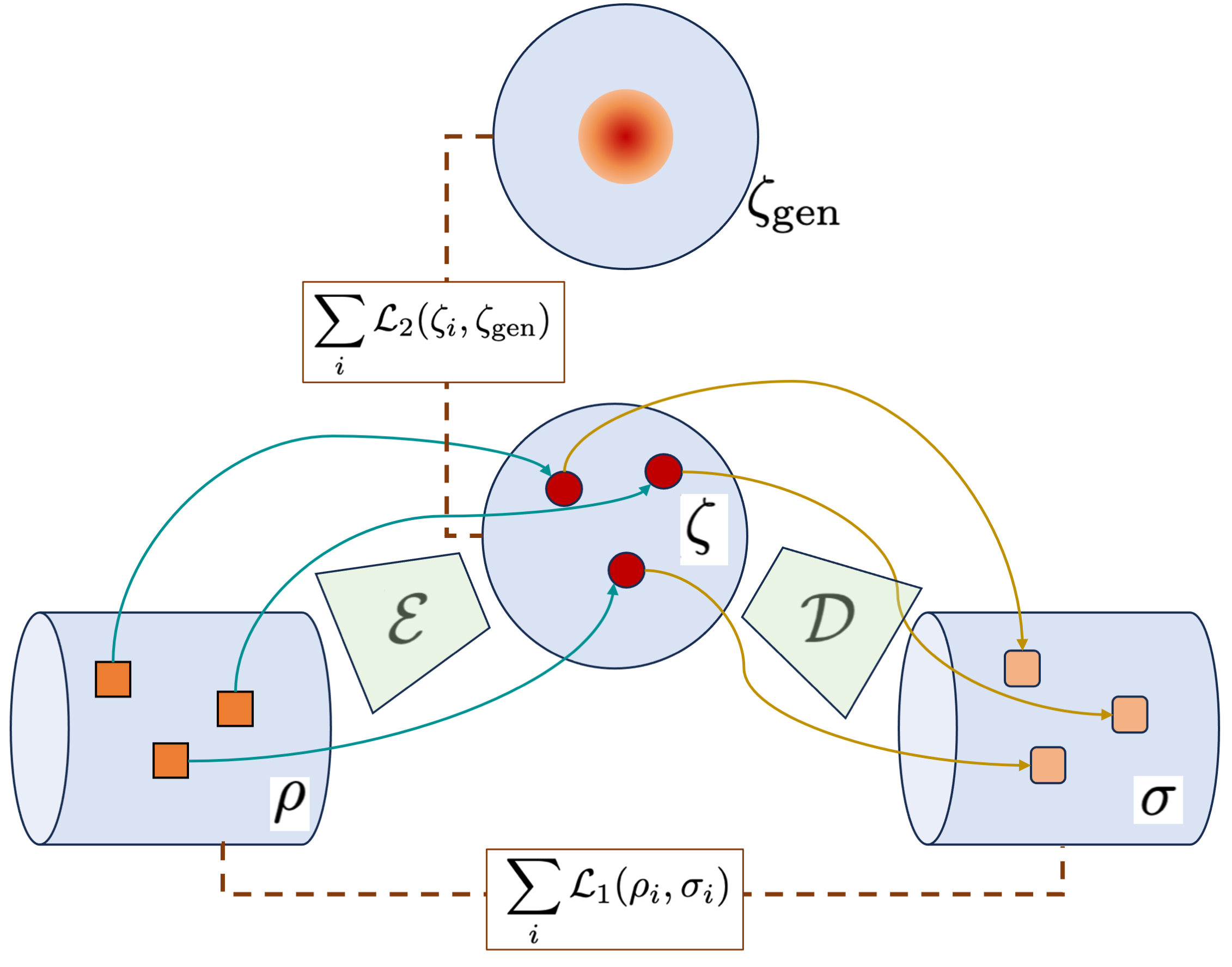
(a)

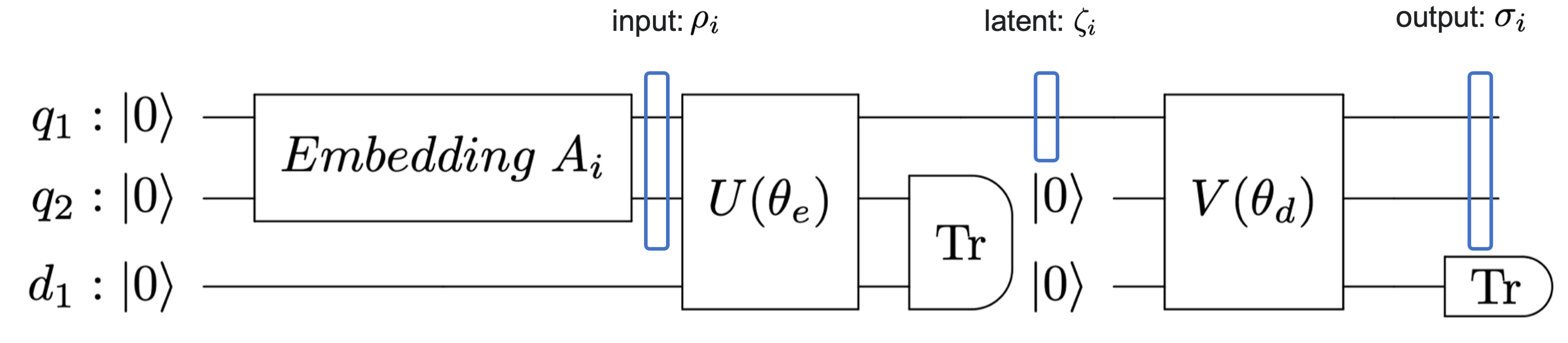
(b)

Figure 1: (a) Illustration of the architecture and objective function of the $\zeta$-QVAE; arrows represent transformations between mixed states, $\zeta_{\text{gen}}$ is the maximally mixed state, and $\mathcal{L}_{1}$ and $\mathcal{L}_{2}$ are the reconstruction and regularization loss respectively. (b) $\zeta$-QVAE overall circuit representation.

In Fig. 2, the encoder circuit $U(\theta_{e})$ we used in this study is shown for one trainable layer $\it{i.e.}\,N_{l}=1$ (note that we use a data embedding circuit, $A_{i}$, to first project classical data to a quantum state, e.g. via amplitude encoding; this is not formally part of the $\zeta$-QVAE encoder, and can be removed if a quantum data source provides the input state). The Ansatz (marked in beige) was introduced by [18] and contains $R_{zz}$ entangling gates and single qubit $R_{y}$ rotations. The decoder circuit contains the same Ansatz as the encoder.

@C=1em @R=.7em & q_1: |0⟩ 1Embedding   A_i 1R_zz(θ_1) 2R_zz(θ_3)R_y(θ_4)
q_2: |0⟩ Embedding   A_i R_zz(θ_1) 1R_zz(θ_2)R_y(θ_5)
d_1: |0⟩ R_zz(θ_2) R_zz(θ_3)R_y(θ_6)1437.7em–

Figure 2: Encoder circuit

3.2 Training objectives

Reconstruction loss, $\mathcal{L}_{1}$: We provide here the explicit forms of all the divergences we consider for the reconstruction loss. As in Sec. 2, a divergence between two density matrices $\rho$ and $\sigma$ over the same Hilbert space is a non-negative function, $\mathcal{L}(\rho,\sigma)$, which is zero iff $\rho=\sigma$, but unlike a metric, need not be symmetric. For generality, we write all divergences below for arbitrary $\rho$ and $\sigma$. However, we are particularly interested in the cases $\mathcal{L}(\rho_{\text{glob}},\sigma_{\text{glob}})$ and $\mathcal{L}(\rho_{i},\sigma_{i})$, denoting the divergence between input and output density matrices for the global and instance level objectives respectively (see Sec. 2 and Sec. 2). For these cases, $\rho_{i}=\ket{\psi_{i}}\bra{\psi_{i}}$, where $\ket{\psi_{i}}$ is the state vector of the $i$-th input data-point, $\rho_{\text{glob}}=(1/N)\sum_{i}\rho_{i}$, $\sigma_{i}=\mathcal{D}(\mathcal{E}(\rho_{i}))$, and $\sigma_{\text{glob}}=\mathcal{D}(\mathcal{E}(\rho_{\text{glob}}))$, where $\mathcal{E}$ and $\mathcal{D}$ are the quantum operation representations of the encoder and decoder, as in Sec. 2. The particular losses we consider for the reconstruction loss, $\mathcal{L}_{1}(\rho,\sigma)$, are summarized below:

• Fidelity loss:

  $$\mathcal{L}^{f}_{1}(\rho,\sigma)=1-\left(\Tr\sqrt{\sqrt{\sigma}\rho\sqrt{\sigma}}\right)^{2},$$ (12)

  where, for a pure state $\rho=\ket{\psi_{\rho}}\bra{\psi_{\rho}}$, this reduces to: $\mathcal{L}^{f}_{1}(\rho,\sigma)=\bra{\psi_{\rho}}\sigma\ket{\psi_{\rho}}$.

• Quantum relative entropy (KLD):

  $$\mathcal{L}^{kl}_{1}(\rho,\sigma)=S(\rho|\sigma)=S(\rho,\sigma)-S(\rho)=-\Tr(\rho\log(\sigma))-S(\rho),$$ (13)

  where $S(\rho)=-\Tr(\rho\log(\rho))$ and $S(\rho,\sigma)=-\Tr(\rho\log(\sigma))$ .

• Symmetric quantum relative entropy (JSD) [15]:

  $$\mathcal{L}^{jsd}_{1}(\rho,\sigma) = S\Big{(}\rho\;\Big{|}\;\frac{1}{2}\left[\rho+\sigma\right]\Big{)}+S\Big{(}\sigma\;\Big{|}\;\frac{1}{2}\left[\rho+\sigma\right]\Big{)}.$$ (14)

• Quantum Wasserstein-distance loss:

  $$\mathcal{L}^{w}_{1}(\rho,\sigma)=\min_{\mathcal{T}:\mathcal{T}(\rho)=\sigma}\Tr(\pi(\rho,\mathcal{T})C),$$ (15)

  where $\mathcal{T}$ is a quantum operation, and:

  $$\pi(\rho,\mathcal{T}) \coloneqq \sum_{i}p_{i}(\mathcal{T}(\ket{e_{i}}\bra{e_{i}}))\otimes(\ket{e_{i}}\bra{e_{i}})$$ (16)

  with $\ket{e_{i}}$ an orthogonal basis for $\rho$, hence $\rho=\sum_{i}p_{i}\ket{e_{i}}\bra{e_{i}}$, and $C$ is defined as in [16]. As discussed in Sec. 2, we introduce the following auxiliary loss function in place of $\mathcal{L}^{w}_{1}$ for the reconstruction loss when using the Quantum Wasserstein-distance:

  $$(\mathcal{L}^{\prime}_{1})^{w}(\rho,\mathcal{E},\mathcal{D})=\Tr(\pi(\rho,\mathcal{D}\circ\mathcal{E})C),$$ (17)

  Clearly, we have:

  $$\min_{\begin{subarray}{c}\mathcal{E},\mathcal{D}\\ \text{s.t.}\mathcal{D}(\mathcal{E}(\rho))=\sigma\end{subarray}}(\mathcal{L}^{\prime}_{1})^{w}(\rho,\mathcal{E},\mathcal{D})=\mathcal{L}^{w}_{1}(\rho,\sigma),$$ (18)

  and so we can use the alternative form of the training objectives in Sec. 2 to optimize $\mathcal{L}^{w}_{1}(\rho,\sigma)$.

Regularization loss, $\mathcal{L}_{2}$: We write the regularization loss below in the general form $\mathcal{L}_{2}(\zeta,\zeta_{\text{gen}})$, i.e. a divergence between a mixed-state latent representation $\zeta$ and the analog of the classical generative ‘prior’ on the latent space, $\zeta_{\text{gen}}$. As discussed in Sec. 2, we use $\zeta_{\text{gen}}=\frac{1}{\lambda}I$, where $I$ is the identity operator and $\lambda$ the dimension of the latent Hilbert space. This represents the maximally mixed state, $\it{i.e.}\,$ the quantum state with the maximal entropy. In principle, all the divergences above could be used for the regularization loss, $\mathcal{L}_{2}$. However, we exclude the quantum Wasserstein loss, since this would require us to minimize over an auxiliary circuit to find the lowest-cost transformation $\mathcal{T}$ between $\zeta$ and $\zeta_{\text{gen}}$. We briefly summarize the remaining divergences used for $\mathcal{L}_{2}$, with the simplifications induced by setting $\zeta_{\text{gen}}=\frac{1}{\lambda}I$.

• Fidelity loss:

  $$\mathcal{L}^{f}_{2}(\zeta,\zeta_{\text{gen}})=1-\left(\Tr\sqrt{\sqrt{\zeta_{\text{gen}}}\zeta\sqrt{\zeta_{\text{gen}}}}\right)^{2}.$$ (19)

• Quantum relative entropy (KLD):

  $$\mathcal{L}^{kl}_{2}(\zeta,\zeta_{\text{gen}})=S(\zeta,\zeta_{\text{gen}})-S(\zeta)=\Tr(\zeta\log(\zeta))-\log(1/\lambda)=-S(\zeta)+c,$$ (20)

  where $c=-\log(1/\lambda)$.

• Symmetric quantum relative entropy (JSD):

  $$\mathcal{L}^{jsd}_{2}(\zeta,\zeta_{\text{gen}}) = S\Big{(}\zeta\;\Big{|}\;\frac{1}{2}\left[\zeta+\zeta_{\text{gen}}\right]\Big{)}+S\Big{(}\zeta_{\text{gen}}\;\Big{|}\;\frac{1}{2}\left[\zeta+\zeta_{\text{gen}}\right]\Big{)}$$ (21)

Overall training objectives: For explicitness, we collect together the specific forms of the overall global and instance based training objectives used to train our model, based on Sec. 2 and Sec. 2 respectively:

$$\mathcal{L}_{\text{glob}}(\theta_{e},\theta_{d},\beta) = \mathcal{L}_{1}(\rho_{\text{glob}},\sigma_{\text{glob}})+\beta\mathcal{L}_{2}(\zeta_{\text{glob}},\zeta_{\text{gen}})$$

$$\mathcal{L}_{\text{inst}}(\theta_{e},\theta_{d},\beta) = \sum_{i}\left(\mathcal{L}_{1}(\rho_{i},\sigma_{i})+\beta\mathcal{L}_{2}(\zeta_{i},\zeta_{\text{gen}})\right)$$ (22)

along with the alternative forms used for the Wasserstein reconstruction loss based on Sec. 2 and Eq. 17:

$$\mathcal{L}^{\prime}_{\text{glob}}(\theta_{e},\theta_{d},\beta) = \mathcal{L}^{\prime}_{1}(\rho_{\text{glob}},\mathcal{E}(\theta_{e}),\mathcal{D}(\theta_{d}))+\beta\mathcal{L}_{2}(\zeta_{\text{glob}},\zeta_{\text{gen}})$$

$$\mathcal{L}^{\prime}_{\text{inst}}(\theta_{e},\theta_{d},\beta) = \sum_{i}\left(\mathcal{L}^{\prime}_{1}(\rho_{i},\mathcal{E}(\theta_{e}),\mathcal{D}(\theta_{d}))+\beta\mathcal{L}_{2}(\zeta_{i},\zeta_{\text{gen}})\right).$$ (23)

3.3 QSVC classifier

In addition to the ability of the $\zeta$-QVAE to reconstruct the original states, we are also interested in how well the latent and reconstructed states belonging to different classes can be effectively distinguished. In other words, we want to evaluate the classification performance on the latent and reconstructed states in comparison to the original input states. To evaluate this, we implemented a quantum kernel based classifier[18] with amplitude embedding.

Our QSVC classifier is illustrated in Fig. 3 using an example with one trainable layer. We use the same Ansatz, which includes alternating $R_{zz}$ and $R_{y}$ gates for the quantum kernel, as employed in the encoder and decoder. The similarity kernel of our QSVC is obtained as the quantum fidelity between each data pair. Due to the nature of the gene expression data and the normalizations we applied to our data for the amplitude embedding, we have observed a concentration of fidelity scores towards the higher end rather than being spread across the entire range from zero to one. To address this, we introduced a scaling function

$$f\Big{(}\bra{v_{i}}\ket{v_{j}}\Big{)}=\tan\Big(\frac{\pi}{2.03}\bra{v_{i}}\ket{v_{j}}\Big{missing})$$

to enhance resolution within the densely populated region.

@C=1em @R=.7em & q_1: |0⟩ 2Embedding   A_i 1R_zz(θ_1) 2R_zz(θ_3)R_y(θ_4) 2QSVC
q_2: |0⟩ Embedding   A_i R_zz(θ_1) 1R_zz(θ_2)R_y(θ_5)QSVC
q_3: |0⟩ Embedding   A_i R_zz(θ_2) R_zz(θ_3)R_y(θ_6)QSVC1437.7em–

Figure 3: The overall QSVC architecture.

4 Experiments

4.1 Dataset

We test our model on a synthetic dataset that is designed to be compressible and a large and noisy real-world gene expression dataset (including schizophrenia patients and controls) from the PsychENCODE project [19].

4.1.1 PsychENCODE gene expression data

In this dataset, the schizophrenia status for patients and controls is given together with the quantile normalized expression values of 16 selected genes, generated from RNAseq data from the prefrontal cortex of $\sim 1500$ postmortem subjects from the PsychENCODE consortium [19]. These genes were selected from a panel of 555 genes, including pre-identified high-confidence schizophrenia genes and transcription factors. The 16 genes selected were those found to have the highest variance across patients.

To allow for possible future applications of angle embedding on this dataset, we first conducted a global normalization on the data

$$\vec{x}_{i}\rightarrow\pi\times[\vec{x}_{i}-\min(X)]/[\max(X)-\min(X)],$$

where $X$ is the entire dataset matrix (including all feature vectors from all data points) and $\vec{x}_{i}$ the gene expression vector of the $i$-th data point. We employed amplitude embedding in this study; we therefore performed an additional per-data-point L2 normalization, which allowed us to process the data as state vectors. We randomly picked equal number of cases (patients) and controls to create a training and test partition of size 695 and 298 respectively.

4.1.2 Swiss Roll synthetic dataset

In the interest of understanding the generalizability to different datasets, we run the $\zeta$-QVAE and QSVC classifier on $1000$ data points from the Swiss Roll dataset [20] as implemented in Python’s scikit-learn package. The Swiss Roll dataset involves a helically distributed sheet of 3-dimensional points that can be compressed to a 2-dimensional manifold. To adapt the dataset to our context, we take the 3-dimensional dataset and append 5 additional dimensions by adding Gaussian-distributed noise terms (zero-centered, standard deviation $=0.2$). We applied a per-data-point L2 normalization to make the inputs suitable for the quantum circuit. Furthermore, we set up a classification task by designating approximately half of the points as “cases" and the other half as “controls"; the task is designed to allow perfect classification along the 2-dimensional manifold, thus serving to evaluate how well we capture the 2-dimensional manifold.

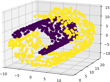
Figure 4: The 3-dimensional Swiss Roll dataset. The colors indicate the labels for the classification task.

4.2 Model setup

To train the $\zeta$-QVAE, we employed the COBYLA optimizer, utilizing a training duration of 60 epochs with a patience setting of 20 epochs throughout the study. Additionally, we kept the number of layers $N_{l}$ identical within both the encoder and decoder, as well as the count of auxiliary qubits in the encoder and decoder ($N_{A}$ and $N_{B}$). When running the $\zeta$-QVAE with $N_{T}$ trash qubits, we select the first $N_{T}$ qubits as trash qubits. All the performance results, including $\zeta$-QVAE reconstruction rate and QSVC classification accuracies are averaged over five random initializations.

We determined the number of layers of the QSVC classifier $N_{cl}$ based on its performance on the input datasets. Notably, we observed that varying $N_{cl}$ between one and three had negligible impact for the datasets comprising 16 input features. Nevertheless, to account for potential larger input feature dimensions, where a greater $N_{cl}$ might be essential, we opted to set $N_{cl}=3$ for the remainder of the study. Throughout this study, the test accuracy serves as the metric for the classification performance.

5 Results

In this section, we begin by subsec. 5.1 offering an overview of different objective functions introduced in subsec. 3.2. Subsequently, we focus on the specific case of our model in which the negative fidelity serves as the reconstruction loss, complemented by the JSD as the regularization loss. We will refer to this specific objective function as Fid+JSD in the following. In subsec. 5.2 and subsec. 5.3, we provide a thorough investigation of the impact of the model architecture on the regularization, and consequently, on the quantum state reconstruction and downstream classification tasks using the Fid+JSD objective function. In subsec. 5.4 we test our framework with the global level objective function. Then in subsec. 5.5, we test the $\zeta-$QVAE on the synthetic dataset. Finally in subsec. 5.6, we compare the $\zeta-$QVAE with QAE and classical VAE models.

In our model, the architecture is controlled by several hyperparameters, including the number of layers $N_{l}$ in the encoder and decoder, the $\beta$-value and the number of auxiliary qubits in the encoder and decoder $N_{A}=N_{B}$. As we show, the impacts of these hyperparameters are not independent from each other. We evaluate the performance of each model using the fidelity reconstruction rate of the $\zeta$-QVAE and the accuracy of the QSVC on the downstream classification tasks. The notation employed in this section is as follows: $f(N_{A},N_{l})$ represents the fidelity reconstruction rate of a given model with $N_{A}$ auxiliary qubits and $N_{l}$ layers. Similarly, $l(N_{A},N_{l})$ signifies the QSVC test accuracy using the latent states of the corresponding model with $N_{A}$ auxiliary qubits and $N_{l}$ layers as input, while $r(N_{A},N_{l})$ denotes the QSVC test accuracy using the reconstructed states as input.

5.1 Objective function choice:

Choice of reconstruction loss We begin with the evaluation of the three different forms of reconstruction loss - fidelity, Wasserstein and JSD - at $\beta=0$, which implies that the regularization term is excluded from the objective function. The results are presented in Tab. 1.

Table 1: Comparison of the three types of reconstruction losses at $\beta=0$.

	fidelity	wasserstein	JSD
$f(0,3)$	$0.844\pm 0.043$	$0.853\pm 0.033$	$0.839\pm 0.037$
$l(0,3)$	$0.647\pm 0.01$	$0.652\pm 0.007$	$0.652\pm 0.013$
$r(0,3)$	$0.644\pm 0.01$	$0.65\pm 0.005$	$0.653\pm 0.012$
$f(0,2)$	$0.898\pm 0.008$	$0.882\pm 0.013$	$0.875\pm 0.012$
$l(0,2)$	$0.636\pm 0.008$	$0.65\pm 0.009$	$0.653\pm 0.011$
$r(0,2)$	$0.637\pm 0.008$	$0.65\pm 0.01$	$0.654\pm 0.007$
$f(0,1)$	$0.953\pm 0$	$0.771\pm 0.223$	$0.953\pm 0.0$
$l(0,1)$	$0.606\pm 0.002$	$0.62\pm 0.019$	$0.605\pm 0.002$
$r(0,1)$	$0.607\pm 0.003$	$0.622\pm 0.023$	$0.606\pm 0.005$
$f(1,3)$	$0.742\pm 0.046$	$0.695\pm 0.024$	$0.686\pm 0.048$
$l(1,3)$	$0.655\pm 0.003$	$0.65\pm 0.008$	$0.651\pm 0.005$
$r(1,3)$	$0.627\pm 0.021$	$0.607\pm 0.026$	$0.63\pm 0.016$
$f(1,2)$	$0.851\pm 0.029$	$0.838\pm 0.026$	$0.841\pm 0.03$
$l(1,2)$	$0.653\pm 0.013$	$0.657\pm 0.011$	$0.653\pm 0.014$
$r(1,2)$	$0.613\pm 0.019$	$0.601\pm 0.023$	$0.622\pm 0.019$
$f(1,1)$	$0.886\pm 0.009$	$0.894\pm 0.005$	$0.9\pm 0.007$
$l(1,1)$	$0.629\pm 0.018$	$0.64\pm 0.027$	$0.636\pm 0.023$
$r(1,1)$	$0.574\pm 0.021$	$0.573\pm 0.03$	$0.571\pm 0.032$

We found that all three types of reconstruction loss behave qualitatively similarly at $\beta=0$, which can be briefly summarized as follows (further details are elaborated in subsec. 5.2 and subsec. 5.3):

• In the case no auxiliary qubits are employed in the decoder, the reconstructed state is identical to the latent state (extended by reference $\ket{0}$ trash-qubits) up to a unitary transformation and thus results in substantially the same fidelity-based quantum kernel matrix for QSVC. Thus, the classification performance on the latent and reconstructed states is observed to be effectively the same.

• Regardless of the presence of auxiliary qubits, with an increasing number of layers, the fidelity reconstruction rate decreases while the test accuracy of classification tasks improves for both latent and reconstructed states. This observation implies that increasing the number of layers may implicitly regularize the model, since the larger parameter search space increases the difficulty for the COBYLA optimizer of finding solutions with high reconstruction fidelity.

• For any given value of $N_{l}$, incorporating auxiliary qubits results in a lower fidelity reconstruction rate compared to the case where no auxiliary qubits are used. However, the classification accuracy on the latent states improves slightly while the classification accuracy on the reconstructed states drops especially for smaller $N_{l}$.

We observe that, generally, the negative fidelity loss is able to achieve better reconstruction performance, while performing comparably to the other losses on classification tasks; we therefore use fidelity reconstruction loss in the following sections.

Choice of regularization loss: Next, we examine the different choices of regularization loss choices at different values of $\beta$. The results are shown in 2(c). Given the variations in overall scale among the different forms of regularization loss, our focus shifts to slightly different ranges of $\beta$ for each. Recalling the baseline results at $\beta=0$ from Tab. 1, the performance of the fidelity reconstruction loss is as follows: $f(0,3)=0.844\pm 0.043$, $l(0,3)=0.647\pm 0.01$ and $r(0,3)=0.644\pm 0.01$.

Table 2: Negative fidelity reconstruction loss with three different regularization loss options.

	$\beta=0.5$	$\beta=1$	$\beta=1.5$	$\beta=2$	$\beta=2.2$	$\beta=2.5$	$\beta=2.7$
$f(0,3)$	$0.876\pm 0.025$	$0.843\pm 0.02$	$0.813\pm 0.017$	$0.815\pm 0.013$	$0.763\pm 0.043$	$0.765\pm 0.038$	$0.728\pm 0.035$
$l(0,3)$	$0.651\pm 0.007$	$0.651\pm 0.011$	$0.654\pm 0.012$	$0.653\pm 0.009$	$0.658\pm 0.005$	$0.669\pm 0.005$	$0.661\pm 0.011$
$r(0,3)$	$0.653\pm 0.005$	$0.649\pm 0.009$	$0.652\pm 0.01$	$0.655\pm 0.01$	$0.661\pm 0.005$	$0.665\pm 0.003$	$0.061\pm 0.011$

(a) JSD regularization loss

	$\beta=0.5$	$\beta=1$	$\beta=1.5$	$\beta=2$	$\beta=2.2$	$\beta=2.5$
$f(0,3)$	$0.773\pm 0.039$	$0.714\pm 0.037$	$0.664\pm 0.064$	$0.522\pm 0.085$	$0.53\pm 0.076$	$0.425\pm 0.068$
$l(0,3)$	$0.654\pm 0.014$	$0.653\pm 0.012$	$0.652\pm 0.009$	$0.653\pm 0.014$	$0.656\pm 0.009$	$0.661\pm 0.007$
$r(0,3)$	$0.654\pm 0.011$	$0.652\pm 0.012$	$0.652\pm 0.008$	$0.65\pm 0.014$	$0.658\pm 0.014$	$0.661\pm 0.007$

(b) KLD regularization loss

	$\beta=0.5$	$\beta=1$	$\beta=1.1$	$\beta=1.2$	$\beta=1.5$	$\beta=2$	$\beta=2.5$
$f(0,3)$	$0.863\pm 0.009$	$0.864\pm 0.025$	$0.847\pm 0.015$	$0.849\pm 0.015$	$0.834\pm 0.027$	$0.829\pm 0.033$	$0.798\pm 0.03$
$l(0,3)$	$0.648\pm 0.007$	$0.646\pm 0.015$	$0.657\pm 0.008$	$0.661\pm 0.01$	$0.655\pm 0.005$	$0.653\pm 0.008$	$0.648\pm 0.019$
$r(0,3)$	$0.649\pm 0.007$	$0.646\pm 0.014$	$0.658\pm 0.01$	$0.658\pm 0.01$	$0.657\pm 0.006$	$0.656\pm 0.01$	$0.651\pm 0.018$

(c) Negative fidelity regularization loss

Here, we observe that KLD has the least favorable performance among the regularization loss options in terms of reconstruction rate. All three regularization loss options seem to be comparable in classification test accuracy, although the model utilizing JSD performs is slightly better for the optimal $\beta$. Consequently, our focus in the next section is on the combination of negative fidelity reconstruction loss and JSD regularization loss.

5.2 Understanding the determinants of regularization and reconstruction in $\zeta-$QVAE

Models with appropriately tuned regularization, leading to an optimal degree of disentanglement in their latent representations, have been shown to outperform those lacking such adjustments due to their ability to capture the independent underlying latent factors effectively [1]. In this section, we investigate how the degree of regularization (explicit and implicit, as discussed below) and the reconstruction rate of the $\zeta-$QVAE are influenced by the interplay of several factors: the $\beta$-value, the presence of auxiliary qubits and the circuit complexity. We impose different circuit complexity constraints by varying the number of layers $N_{l}$ in the encoder and decoder and studied a range of $\beta$-values from zero to six, while considering all combinations with and without one auxiliary qubit.

The reconstruction ability of the model is estimated using the fidelity reconstruction rate. To quantify the regularization effect, we analyze the distribution of the latent states in the latent space by calculating the regularization loss. In addition, we take into account downstream classification performance as an additional metric for the evaluation of the reconstruction rate and degree of regularization.

Table 3: Fid+JSD objective function

	$\beta=0$	$\beta=1$	$\beta=2$
$f(0,3)$	$0.844\pm 0.043$	$0.843\pm 0.02$	$0.815\pm 0.013$
$l(0,3)$	$0.647\pm 0.01$	$0.651\pm 0.011$	$0.653\pm 0.009$
$r(0,3)$	$0.644\pm 0.01$	$0.649\pm 0.009$	$0.655\pm 0.01$
$f(0,2)$	$0.898\pm 0.008$	$0.883\pm 0.018$	$0.832\pm 0.027$
$l(0,2)$	$0.636\pm 0.008$	$0.644\pm 0.009$	$0.653\pm 0.009$
$r(0,2)$	$0.637\pm 0.008$	$0.644\pm 0.004$	$0.655\pm 0.007$
$f(0,1)$	$0.953\pm 0.0$	$0.673\pm 0.212$	$0.728\pm 0.186$
$l(0,1)$	$0.606\pm 0.002$	$0.646\pm 0.006$	$0.653\pm 0.008$
$r(0,1)$	$0.607\pm 0.003$	$0.647\pm 0.003$	$0.653\pm 0.01$
$f(1,3)$	$0.742\pm 0.046$	$0.649\pm 0.061$	$0.561\pm 0.066$
$l(1,3)$	$0.655\pm 0.003$	$0.651\pm 0.011$	$0.651\pm 0.016$
$r(1,3)$	$0.627\pm 0.021$	$0.613\pm 0.004$	$0.605\pm 0.011$
$f(1,2)$	$0.851\pm 0.029$	$0.815\pm 0.03$	$0.686\pm 0.044$
$l(1,2)$	$0.653\pm 0.013$	$0.638\pm 0.01$	$0.644\pm 0.005$
$r(1,2)$	$0.613\pm 0.019$	$0.6\pm 0.027$	$0.593\pm 0.024$
$f(1,1)$	$0.886\pm 0.009$	$0.887\pm 0.009$	$0.887\pm 0.006$
$l(1,1)$	$0.629\pm 0.018$	$0.648\pm 0.005$	$0.648\pm 0.012$
$r(1,1)$	$0.574\pm 0.021$	$0.588\pm 0.014$	$0.562\pm 0.022$

We noticed that the models with $N_{l}=1$ and no auxiliary qubits often failed to converge at non-zero $\beta$ values, leading to the large standard deviation of $f(0,1)$ in Tab. 3. For example, among the five random initializations at $\beta=2$, two exhibited a test fidelity reconstruction rate around $0.5$ while the remaining three had a fidelity of approximately 0.88. Similarly, at $\beta=1$, three had fidelity around 0.5, and the remaining two showed a fidelity near 0.93. Further, for the models with $N_{l}=1$ and one auxiliary qubit, we found that for the range of $\beta\in[0,6]$, the reconstruction fidelity remained constant within the error range as suggested by $f(1,1)$ in Tab. 3. Below we provide several key findings based on results obtained for $N_{l}=2$ and 3.

Regularization is controlled by $\beta$-value, model complexity and number of auxiliary qubits: Varying $\beta$ is the most direct way to adjust the degree of the regularization. In Fig. 5, the fidelity reconstruction rate (which is 1 for a perfect reconstruction) and regularization loss (where 0 implies stronger regularization / smaller regularization loss) are shown as a function of $\beta$. We see that for the entire range of $\beta$ considered in this study, higher $\beta$ values lead to stronger regularization and worse fidelity reconstruction rates. One can also see in Fig. 5, that the regularization loss is smaller when using one auxiliary qubit compared to the scenario without any auxiliary qubits, across all values of $\beta$. In addition, the model complexity controlled by $N_{l}$ can also influence the degree of the regularization. As we can see in Tab. 3 in the case where no auxiliary qubits are present, similar to our observation at $\beta=0$, increasing the number of layers in the encoder and decoder also leads to a decreased reconstruction rate for $\beta=1$ and 2, accompanied by improved classification performance. Increasing the number of layers or the number of auxiliary qubits thus has a similar effect to increasing $\beta$, resulting in a form of implicit regularization as noted above in subsec. 5.1. At $\beta=0$, the effect of increasing number of layers is more noticeable than at a higher value of $\beta$. The number of layers, auxiliary qubits and $\beta$ can thus be viewed as jointly contributing to the regularization of the model.

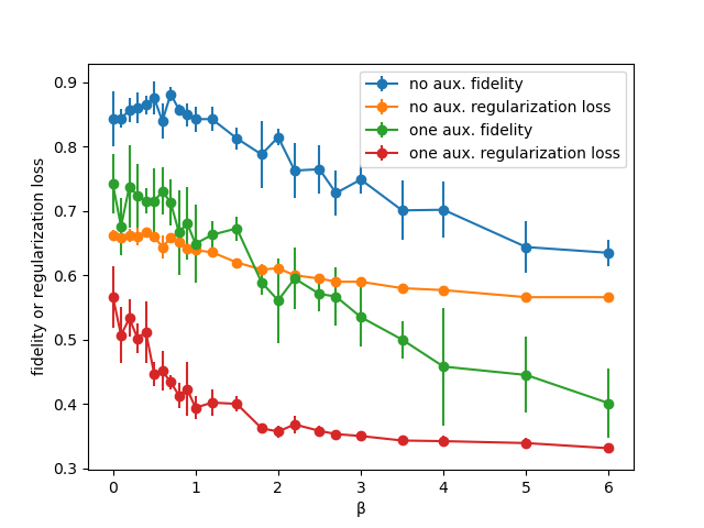
Figure 5: The two components of the objective function are plotted as a function of $\beta$ for the case with one trash qubit and $N_{l}=3$.

Reconstruction and regularization are strongly dependent in the absence of auxiliary qubits: In the case where no auxiliary qubits are used, the reconstructed states are obtained from the latent states by a unitary (linear) operation. This means effectively, both the reconstruction constraints and the regularization constraints are imposed to the same space (since the latent states are mapped to a linear subspace of the output space with the same intrinsic dimensionality). The reconstructed state thus inherits directly the same regularization as the latent state. This can be seen in the left panels in Fig. 6, where a lower reconstruction loss at smaller $\beta$ can only be achieved by sacrificing the regularization loss, $\it{i.e.}\,$ by allowing a higher regularization loss.

Reconstruction and regularization are substantially decoupled in the presence of auxiliary qubits: In the presence of auxiliary qubits, we observed simultaneous decreasing curves for the regularization loss and the reconstruction loss in right panels of Fig. 6 (one should note that the reconstruction loss is the negative counterpart of the reconstruction fidelity shown in Fig. 5). This is because the presence of auxiliary qubits allows for non-unitary transformations from latent states to reconstructed states, thus allowing a separate optimization of the regularization loss and reconstruction loss. This feature of $\zeta-$QVAE has no classical analogue and can be potentially utilized to devise a framework for controlling the degree of coupling between latent and reconstructed states, thus enabling a flexible trade-off between regularization and reconstruction rates.

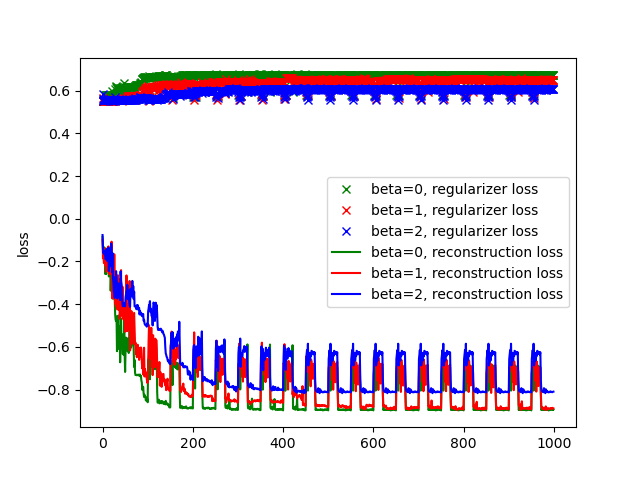
(a) $N_{l}=2$, no auxiliary qubits

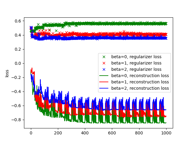
(b) $N_{l}=2$, one auxiliary qubit

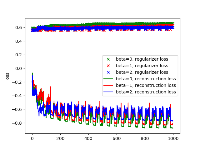
(c) $N_{l}=3$, no auxiliary qubits

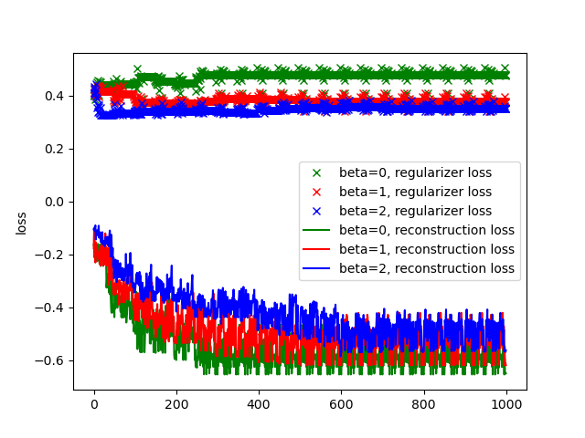
(d) $N_{l}=3$, one auxiliary qubit

Figure 6: The optimization process of the reconstruction loss and regularization loss are shown separately. In the absence of auxiliary qubits, the two components of the objective function are mutually dependent. Utilizing auxiliary qubits allows for decoupling and thus simultaneous improvement of both terms.

Reconstructing the original state poses challenges in the presence of auxiliary qubits: As shown in Tab. 3, the fidelity reconstruction rate is lower in the presence of one auxiliary qubit compared to its absence. In addition, we note a decrease in the classification performance on the reconstructed states when one auxiliary qubit is used compared to when no auxiliary qubits are used. Whereas for the latent states, the classification performance remains similar. The observed phenomenon may be explained by the removal of the constraint imposed by the coupled reconstruction loss and regularization loss when employing one auxiliary qubit, which introduces a greater challenge to the optimization process of the model parameters[21]. This difficulty in optimization may be exacerbated by the Barren plateau effect intensified by the inclusion of an additional qubit [22].

5.3 Optimal representations for downstream classification tasks

An optimal degree of regularization exists for the downstream classification performance: In Fig. 7 (a) and (b), we plot the downstream classification performance against $\beta$. We noticed that when no auxiliary qubits are used, an optimal range of $\beta$ is associated with higher classification accuracy. For the one trash qubit case, $\it{i.e.}$ $N_{T}=1$, shown in (a), the optimal $\beta$ is found to be around $2.5$ for both $N_{l}=2$ and $N_{l}=3$. We also note that the model using three layers achieved slightly higher classification accuracy than the two-layer model. On the other hand, when one auxiliary qubit is used, the regularization seems to have no clear impact on the downstream classification performance (red and green points). Nevertheless, we cannot conclude less significant improvements cannot be identified since there is a large range of uncertainty in the performance. In panel (b) where two trash qubits are used, the optimal $\beta$ occurs around 2 for the scenario without auxiliary qubits. Although it is still difficult to determine if there exists an optimal range of $\beta$ in the scenarios with one auxiliary qubit, we can see that the performance of the models with auxiliary qubits is slightly better than that without auxiliary qubits.

In panels (c) and (d), we plot the test accuracy directly against the regularization loss. For both $N_{T}=1$ and $N_{T}=2$ without auxiliary qubits, we see a clear optimal range of regularization loss at 0.6 (for $N_{T}=1$) and 0.11 (for $N_{T}=2$). For models with auxiliary qubits, we included also negative $\beta$s, indicated by green points. This is motivated by the observation that, even for $\beta=0$, the regularization was already stronger than the optimal range observed for cases without auxiliary qubits case (blue points). As shown in (c), $l(1,3)$ (red points) improves slightly with increasing regularization loss in the $N_{T}=1$ case, and this trend persists with a slight improvement for negative $\beta$ values. In (d), The data suggests an upward trend as the regularization loss decreases. However, this observed trend is less pronounced compared to models without auxiliary qubits and remains suggestive rather than conclusive.

Regularization is more advantageous for smaller latent space: For $N_{T}=1$, the latent space is an eight-dimensional Hilbert space formed by three qubits while for $N_{T}=2$, the latent space is four-dimensional formed by two qubits. As shown in Fig. 7 (a) and (b), for the $N_{T}=1$ case, the regularization improves the classification performance by $\approx 4\%$ while for $N_{T}=2$, the improvement is over $7.5\%$.

Classification performance on the latent states is similar to that on the input states: The classification performance of the employed QSVC on the input states is $0.675\pm 0.003$. For one trash qubit case, $\it{i.e.}$ compressing to half of the original dimensionality, the best classification performance achieved on the latent states is $0.669\pm 0.005$ for $\beta=2.5$, $N_{l}=3$ and no auxiliary qubits. Notably, this is only $0.9\%$ lower than that achieved with the full original states. For two trash qubits, $\it{i.e.}$ compressing to a quarter of the original dimensionality, we achieved a classification performance of $0.63\pm 0.015$ for $\beta=6$, $N_{l}=3$ and one auxiliary qubit.

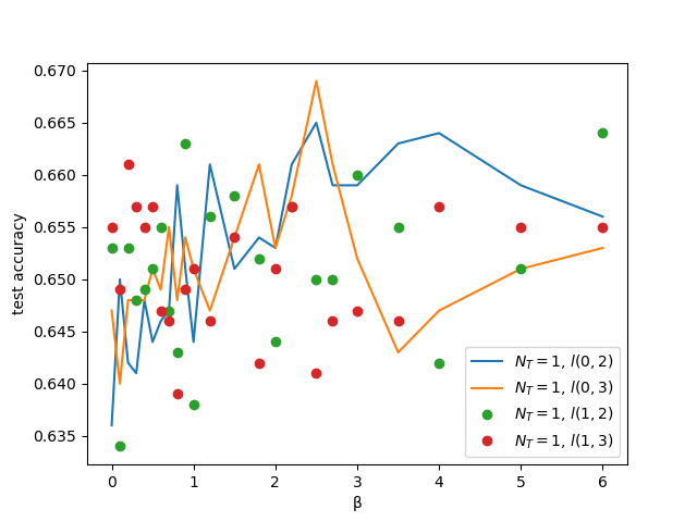
(a) $N_{T}=1$

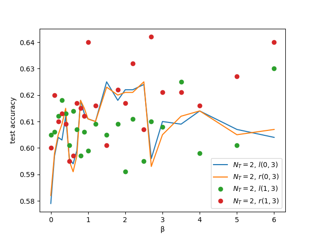
(b) $N_{T}=2$

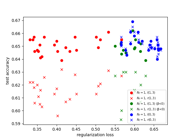
(c) $N_{T}=1$, including negative $\beta$ in green

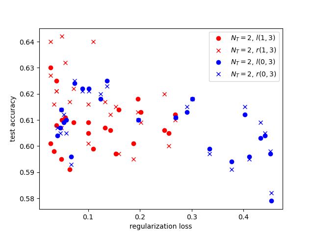
(d) $N_{T}=2$

Figure 7: (a) and (b): Classification performance is plotted against $\beta$. For both $N_{T}=1$ and 2, the no auxiliary qubit cases (orange and blue line) clearly show an optimal $\beta$ with improved classification performance, while in the one auxiliary qubit case the optimal $\beta$ range is unclear. For $N_{T}=2$ using auxiliary qubits is advantageous compared to no auxiliary qubits. (c) and (d): Plots test accuracy directly against regularization loss to eliminate uncertainties caused by the intermediate parameter $\beta$. For both $N_{T}=1$ and 2, while in the no auxiliary qubit case, there is clearly an optimal range for regularization loss, for the one auxiliary qubit case this is less clear.

5.4 Training using global objective

Recall from Eq. 1, that the global state is defined as a mixed state over the entire input dataset. In this section, we test the performance of the $\zeta$-QVAE using the global density matrix. We consider only the setup where negative fidelity serves as the reconstruction loss and JSD acts as regularization loss.

In this scenario, our quantum circuit is trained on a single global input state, while the model construction is identical to that of the instance-level model. Hence, through the training phase, one single latent state and one output state are present. Following the completion of quantum circuit training, each individual instance-level input data point will be fed through the optimized model. For each data point within the original dataset, the associated latent state and reconstructed state are computed. Subsequently, calculations for the fidelity reconstruction rate calculation and downstream classification tasks are executed on the instance-level input, latent and reconstructed states.

We tested a range of $\beta$s on the global $\zeta-$QVAE and the results are shown in Fig. 8. While the reconstruction rate is slightly lower for nearly all $\beta$s, the overall pattern of the curve with respect to $\beta$ is very similar to that of the instance-level trained models. In the down-stream classification tasks, the QSVC test accuracy achieved on the latent and reconstructed states remains comparable for $\zeta-$QVAE models trained on both global and instance-level data. For $l(0,3)$, where an optimal $\beta$ of 2.5 was observed for the instance-level trained models, the globally trained models exhibit an optimal $\beta$ of three. Nevertheless, the disparity in performance falls within the error range.

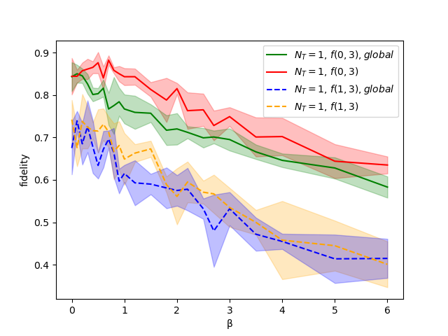
(a) Fidelity reconstruction rate

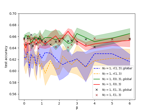
(b) Classification performance

Figure 8: For $N_{T}=1$ and $N_{l}=3$, we compare the globally trained with the instance-level trained model. The shaded areas represent the error range.

5.5 Application to the Swiss Roll dataset

To evaluate performance on the Swiss Roll dataset (Fig. 9), we considered the case where our 8-dimensional input state is mapped to 3 qubits and the latent state is determined by 1 qubit. For the $\zeta$-QVAE, we set $N_{T}=2$, $N_{l}=3$, $\beta=\{0,0.5,1.0,1.5,2.0,2.5,3.0,3.5\}$, and test the scenario with zero auxiliary qubits to one with 1 auxiliary qubit added to the encoder and decoder. The results yield similar conclusions to those of the gene expression dataset. The reconstruction fidelity on the leave-out test set steadily decreases with an increase in $\beta$, irrespective of the number of auxiliary qubits (Fig. 9b). In contrast, the test accuracy in the classification task using the latent state achieves a peak at $\beta=1.5$ for the 0-auxiliary-qubits case, showing an improved test accuracy of $0.75\pm 0.04$ relative to the accuracy of $0.60\pm 0.02$ at $\beta=0$. On the other hand, there is no clear benefit of a non-zero $\beta$ for the 1-auxiliary-qubit case, at least at the values screened here (Fig. 9c). This may be due to the fact that the implicit regularization due to the inclusion of the auxiliary qubit is already quite strong at $\beta=0$. Overall, the test accuracy remains reasonably high, with a maximum of $0.75\pm 0.04$ (based on both the latent and reconstructed states; test AUC = $0.82\pm 0.05$) for 0 auxiliary qubits and $0.77\pm 0.01$ (based on the latent state; test AUC = $0.82\pm 0.02$) for 1 auxiliary qubit.

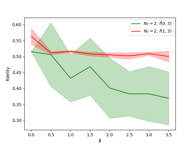
(a) Fidelity reconstruction rate

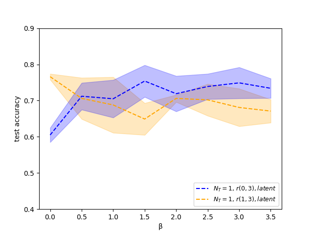
(b) Classification performance

Figure 9: $N_{T}=2$, $N_{l}=3$. We evaluate the performance of the $\zeta$-QVAE (a) and QSVC classifier on the latent states (b) using the Swiss Roll dataset. The shaded areas represent the error range.

5.6 Comparison to QAE and classical VAEs

Quantum Autoencoder (QAE): At $\beta=0$, $\zeta$-QVAE without the regularization term and with a fidelity-based reconstruction loss is similar to the QAE introduced in Ref. [5] with the following minor differences: (1) The objective function to be maximized in Ref. [5], $\it{i.e.}$ fidelity on the trash state $F(\rho_{t},\ket{0})$, serves as an upper bound of the actual reconstruction fidelity $F(\rho_{i},\mathcal{D}(\mathcal{E}(\rho_{i})))$, which we optimize directly; (2) The decoder in QAE is the inverse of encoder, which is a special instance of our decoder, whose parameters are independent from that of the encoder. Our results show that the $\zeta$-QVAE achieves improved classification performance at $\beta>0$, suggesting that models with regularization offer advantages compared to the QAE.

Classical VAEs: We compare two types of classical $\beta$-VAEs [1] to the $\zeta-$QVAE. The first type has a single linear layer without an activation function for both the encoder and decoder. The second type is a two-layer $\beta$-VAE with 12 hidden nodes and a RELU activation function. We consider classical $\beta$-VAEs with 8-, 4-, 2- and 1-dimensional latent spaces. Across these cases, we conducted tests over a wide range of $\beta$ and presented the highest classification performance overall $\beta$s in Tab. 4. It is important to note that in the classical $\beta$-VAE, each dimension in the latent space includes a mean and a variance, resulting in two degrees of freedom per dimension. Therefore, a four/two/one latent dimensional classical VAE is comparable to three/two/one latent qubits in the $\zeta-$QVAE, respectively.

On the gene expression data, the fully quantum compression and classification scheme (QVAE+QSVC) reached a classification accuracy of $0.669\pm 0.005$ using three latent qubits and $0.63\pm 0.015$ with two latent qubits, outperforming the fully classical compression and classification scheme (VAE+SVC). On the synthetic Swiss Roll dataset, the $\zeta-$QVAE with one latent qubit achieved a classification accuracy of $0.77\pm 0.01$, which is slightly higher than that of the classical $\beta-$VAE with one-dimensional latent space.

In addition to the improved classification accuracy on the latent states, the number of parameters used by the $\zeta-$QVAE is also much smaller than that of the classical VAE. For example, in the case of 16 input features, a single-layer classical $\beta-$VAE with a 4-dimensional latent space has 216 free parameters. In contrast, a 3-layer $\zeta-$QVAE has only 60 free parameters for the same input features, but benefits from the high dimensionality of the Hilbert space associated with the latent state. It is also possible that the entanglement between the qubits employed by the model contributes to a reduction in the number of parameters needed for encoding the original data.

Table 4: Classification performance on the latent representations

	gene expression data		Swiss Roll dataset
	linear VAE	standard VAE	linear VAE	standard VAE
latent dim. = 8	$0.653\pm 0.027$	$0.659\pm 0.01$	$-$	$-$
latent dim. = 4	$0.643\pm 0.017$	$0.646\pm 0.006$	$-$	$-$
latent dim. = 2	$0.615\pm 0.01$	$0.612\pm 0.019$	$0.784\pm 0.003$	$0.775\pm 0.006$
latent dim. = 1	$-$	$-$	$0.708\pm 0.004$	$0.768\pm 0.004$

6 Advantages of the $\zeta$-QVAE framework

In general, the application domains of $\zeta-$QVAE are not expected to differ significantly from those of classical VAEs. However, certain distinctive features of $\zeta-$QVAE can offer specific advantages in select applications.

Application to large-scale datasets. Our framework addresses key challenges in applying quantum models to fields involving large-scale datasets by allowing big datasets with large feature spaces to be compressed into a smaller latent space while preserving essential information crucial for downstream analyses, such as classification. This reduces the necessary (quantum) data storage capacity and addresses the limited availability of quantum hardware by allowing subsequent analysis to be carried out by quantum devices with a small number of qubits.

Application to privacy-aware computation. Our formulation of global objectives holds potential for privacy-preserving computation, as it potentially eliminates the need for access to all the original data points during model training. Instead, only the global density matrix may be required, or alternatively samples may be provided from any equivalent quantum ensemble with the same density matrix (for instance, the eigenvectors in the basis which the data density matrix diagonalizes, weighted by their eigenvalues). Given that mixed states are composed of classical mixtures of pure states, which may not necessarily be orthogonal, it is possible for different sets of pure states to yield the same mixed state. As a consequence, the decomposition of a mixed state into an ensemble of pure states is not unique. Consequently, if only the global mixed state density matrix is provided, individual-level data cannot be recovered. Moreover, the global objective also offers potential for application in federated learning. In this scenario, the sub-ensembles of each actor may be transformed independently, as their density matrices can be combined additively to generate the full data matrix.

Application to genomics studies. Combining the specific advantages of our framework, we are particularly driven by potential applications in genomics studies. Genomics studies involve large-scale datasets that are diverse in data modalities and often contain sensitive information. Our framework addresses key challenges in the integration of quantum computing within such domains by: 1. enabling the compression of large-scale data into a compact representation, 2. offering flexible selection of problem-specific objectives for various data types, and 3. providing methods to conceal sensitive training data, for instance in scenarios involving individual-level genomics and clinical data.

7 Implementation on near-term quantum devices

It is important to note that implementing our framework on NISQ hardware presents challenges not addressed in this manuscript, such as implementing circuits to input amplitude-encoded state vectors [23], reading out latent mixed states with sufficient accuracy, and storage of the resulting density matrices. Specifically for our framework, efficient methods are needed for the divergence calculations between pairs of quantum states in the objective function, and for quantum state tomography, which is required for latent state readout and storage. For the latter, while there are several generally applicable approaches based on matrix-state tomography [24], neural-network-based tomography [25, 26], or the efficient calculation of density matrix properties [12], the question remains of how well these methods scale for the states learned by our model. Frameworks like ours, which primarily utilize mixed states, may encounter additional practical difficulties due to the large number of parameters required to fully characterize the state, which in turn would impact the number of state samples needed for accurate readout of the states. In our current simulation-based implementation, the latent states are represented by a small number of qubits, but scaling up could demand the incorporation of additional methods when applied to NISQ hardware.

8 Discussion

We have introduced a novel fully quantum VAE architecture, named $\zeta$-QVAE, which utilizes mixed-state latent representation and provides a flexible framework in which a wide range of quantum reconstruction losses and regularizers can be combined in a unified way. Further, a theoretical analysis can be given of the objective functions we introduce, which optimize quantum analogues of the variation bounds underlying the classical $\beta$-VAE and Wasserstein-AE. A notable feature of our framework is that mixed states are treated analogously to classical distributions, significantly generalizing previous QAE architectures. Our results show that our model outperforms classical and alternative QAE models with matched architectures on reconstruction and classification tasks. Moreover, we show that the ability to fine-tune the regularization of the latent states allows our model to optimize its representations for down-stream classification tasks, and there is a complex interplay between regularization and model architecture (including circuit complexity, latent space dimensionality and the inclusion of auxiliary qubits) in determining performance on downstream tasks. We further show that our model performs consistently well when trained using a global mixed-state to represent the data, as opposed to individual pure states per data point, thus indicating promising application potential in private and federated learning settings.

With such considerations in mind, we propose that our framework may be ideally suited to constructing practical quantum models in application areas involving large-scale, heterogeneous and potentially privacy-aware dataset such as genomics. In future work, we intend to further investigate how to utilize the observed interaction between model architecture, explicit and implicit regularization, and downstream task performance from the point of view of representational complexity [27]. Further, we intend to investigate how explicit privacy guarantees and federated versions of our approach may be derived for training our model based on our global objective. Finally, we will investigate the potential of our model to provide efficient compression of intrinsically quantum sources, and implementations of our approach on quantum hardware.

Code availability

The code to run $\zeta$-QVAE is available at https://github.com/gaoyuanwang1976/QVAE.git.

9 Appendix A

We provide here further details and proofs regarding the theoretical properties of our framework. The first relates to the number of qubits required to achieve arbitrary mappings in our encoder and decoder:

Proposition 1: Setting $N_{A}=N_{B}=N_{Z}$ is sufficient to allow arbitrary pairs of quantum operations $(\mathcal{E},\mathcal{D})$ to be learned in our framework.

Proof: An arbitrary quantum channel may be represented by a Choi matrix of rank between 1 and $\text{dim}\mathcal{X}\cdot\text{dim}\mathcal{Y}$, where $\mathcal{X}$ and $\mathcal{Y}$ are the input and output Hilbert spaces of the channel respectively. For $\mathcal{E}$, the input and output spaces have dimension $2^{N_{X}}$ and $2^{N_{Z}}$ respectively; hence the maximum rank of the Choi matrix is $2^{N_{X}}\cdot 2^{N_{Z}}=2^{N_{X}+N_{Z}}$, corresponding to a system requiring $N_{X}+N_{Z}$ qubits, which can be achieved by setting $N_{A}=N_{Z}$. For $\mathcal{D}$, the input and output spaces are swapped, and so the maximum rank is again $2^{N_{X}+N_{Z}}$, leading to an identical setting for $N_{B}$. ∎

Second, we show that, as in the classical case, the regularized reconstruction loss objective we use is also a lower-bound on the negative quantum relative entropy (the analogue of the classical log-likelihood), when using the quantum relative entropy for both the reconstruction and regularization terms in our objective, and setting $\beta=1$ and $\epsilon=0$.

Proposition 2: $-S(\rho_{\text{glob}}|\sigma_{\text{gen}})\geq-S(\rho_{\text{glob}}|\sigma_{\text{glob}})-S(\zeta_{\text{glob}}|\zeta_{\text{gen}})$

Proof: We let $\rho_{\text{glob}}=\sum_{i}p_{i}\ket{v_{i}}\bra{v_{i}}$, $\zeta_{\text{gen}}=(1/2^{N_{Z}})\sum_{j}\ket{w_{j}}\bra{w_{j}}$ and $\zeta_{\text{glob}}=\mathcal{E}(\rho_{\text{glob}})=\sum_{j}q_{j}\ket{w_{j}}\bra{w_{j}}$. Notice that we choose to express $\zeta_{\text{gen}}$ in the same basis as $\zeta_{\text{glob}}$, which is possible, since the former is the maximally mixed state, which diagonalizes in any basis. We can express the LHS of the proposition as:

$$-S(\rho_{\text{glob}}|\sigma_{\text{gen}}) = \Tr{\rho_{\text{glob}}\log\sigma_{\text{gen}}}+S(\rho_{\text{glob}})$$ (24)

$$= \sum_{i}p_{i}\Tr{\ket{v_{i}}\bra{v_{i}}\log\sigma_{\text{gen}}}+S(\rho_{\text{glob}})$$

To derive the proposition, we will bound each of the summands $\Tr{\ket{v_{i}}\bra{v_{i}}\log\sigma_{\text{gen}}}$. We begin by observing the following:

$$\Tr{\ket{v_{i}}\bra{v_{i}}\sigma_{\text{gen}}} = \mathbb{E}_{j\sim\text{Categ}(1/2^{N_{Z}})}[\Tr{\ket{v_{i}}\bra{v_{i}}\mathcal{D}(\ket{w_{j}}\bra{w_{j}})}]$$

$$= \mathbb{E}_{j\sim\text{Categ}(q_{1}...q_{2^{N_{Z}}}})[\Tr{\ket{v_{i}}\bra{v_{i}}\mathcal{D}(\ket{w_{j}}\bra{w_{j}})}\cdot\frac{2^{-N_{Z}}}{q_{j}}]$$

$$= \Tr{\ket{v_{i}}\bra{v_{i}}\mathbb{E}_{j\sim\text{Categ}(q_{1}...q_{2^{N_{Z}}}})[\mathcal{D}(\ket{w_{j}}\bra{w_{j}})\cdot\frac{2^{-N_{Z}}}{q_{j}}]}$$

Hence, introducing logs and applying Jensen’s trace inequality (lines 2-3), we have:

$$\Tr{\ket{v_{i}}\bra{v_{i}}\log\sigma_{\text{gen}}}$$

$$=\Tr{\ket{v_{i}}\bra{v_{i}}\log\mathbb{E}_{j\sim\text{Categ}(q_{1}...q_{2^{N_{Z}}}})[\mathcal{D}(\ket{w_{j}}\bra{w_{j}})\cdot\frac{2^{-N_{Z}}}{q_{j}}]}$$

$$\geq\Tr{\ket{v_{i}}\bra{v_{i}}\mathbb{E}_{j\sim\text{Categ}(q_{1}...q_{2^{N_{Z}}}})[\log\mathcal{D}(\ket{w_{j}}\bra{w_{j}})\cdot\frac{2^{-N_{Z}}}{q_{j}}]}$$

$$=\Tr{\ket{v_{i}}\bra{v_{i}}\mathbb{E}_{j\sim Q}[\log\mathcal{D}(\ket{w_{j}}\bra{w_{j}})]}-\mathbb{E}_{j\sim Q}[\log q_{j}]+\log 2^{-N_{Z}}$$

$$=\Tr{\ket{v_{i}}\bra{v_{i}}\log\sigma_{\text{glob}}}+S(\zeta_{\text{glob}})-S(\zeta_{\text{gen}})$$ (26)

Substituting Sec. 9 into Eq. 24 and summing across $i$, we thus have:

$$-S(\rho_{\text{glob}}|\sigma_{\text{gen}}) \geq \sum_{i}p_{i}(\Tr{\ket{v_{i}}\bra{v_{i}}\log\sigma_{\text{glob}}}+S(\zeta_{\text{glob}})-S(\zeta_{\text{gen}}))+S(\rho_{\text{glob}})$$ (27)

$$= -S(\rho_{\text{glob}}|\sigma_{\text{glob}})+S(\zeta_{\text{glob}})-S(\zeta_{\text{gen}})$$

and the proposition follows, since $S(\zeta_{\text{glob}}|\zeta_{\text{gen}})=S(\zeta_{\text{gen}})-S(\zeta_{\text{glob}})$. ∎

Finally, we show that our global and local objectives are equivalent for linear divergences in the following sense:

Proposition 3: Our global and local objectives have identical minimizers for $\mathcal{E}$ and $\mathcal{D}$, when they can be expressed in the form given in subsec. 3.2, and $\mathcal{L}^{\prime}_{1}$ and $\mathcal{L}_{2}$ are linear functions their first arguments.

Proof: We can express $\rho_{\text{glob}}=(1/N)\sum_{i}\rho_{i}$, and $\zeta_{\text{glob}}=(1/N)\sum_{i}\mathcal{E}(\rho_{i})=(1/N)\sum_{i}\zeta_{i}$, where $\rho_{i}$ are the pure states associated with each data-point, and $\zeta_{i}$ are the associated mixed-state latent representations. Hence, if $\mathcal{L}^{\prime}_{1}$ and $\mathcal{L}_{2}$ are linear in their first arguments, we have:

$$\mathcal{L}^{\prime}_{\text{glob}}(\theta_{e},\theta_{d},\beta) = \mathcal{L}^{\prime}_{1}(\rho_{\text{glob}},\mathcal{E}(\theta_{e}),\mathcal{D}(\theta_{d}))+\beta\mathcal{L}_{2}(\zeta_{\text{glob}},\zeta_{\text{gen}})$$ (28)

$$= (1/N)\sum_{i}\mathcal{L}^{\prime}_{1}(\rho_{i},\mathcal{E}(\theta_{e}),\mathcal{D}(\theta_{d}))+(1/N)\sum_{i}\beta\mathcal{L}_{2}(\zeta_{i},\zeta_{\text{gen}})$$

$$= (1/N)\mathcal{L}^{\prime}_{\text{inst}}(\theta_{e},\theta_{d},\beta)$$

Hence, the two objectives are equivalent up to the factor $(1/N)$, leading to identical minimizers. ∎

In particular, Prop. 3 implies that setting $\mathcal{L}^{\prime}_{1}$ to the form given in Eq. 17 for the Quantum Wasserstein loss, and $\beta=0$ (or setting $\mathcal{L}_{2}$ to the Quantum Wasserstein loss with respect to the $\zeta_{\text{gen}}$), results in identical global and local optimization problems.

References

- [1] Irina Higgins et al. “beta-vae: Learning basic visual concepts with a constrained variational framework” In International conference on learning representations, 2016
- [2] Ilya Tolstikhin, Olivier Bousquet, Sylvain Gelly and Bernhard Schoelkopf “Wasserstein auto-encoders” In arXiv preprint arXiv:1711.01558, 2017
- [3] Olaf Ronneberger, Philipp Fischer and Thomas Brox “U-net: Convolutional networks for biomedical image segmentation” In Medical Image Computing and Computer-Assisted Intervention–MICCAI 2015: 18th International Conference, Munich, Germany, October 5-9, 2015, Proceedings, Part III 18, 2015, pp. 234–241 Springer
- [4] Jonathan Ho, Ajay Jain and Pieter Abbeel “Denoising diffusion probabilistic models” In Advances in neural information processing systems 33, 2020, pp. 6840–6851
- [5] Jonathan Romero, Jonathan P Olson and Alan Aspuru-Guzik “Quantum autoencoders for efficient compression of quantum data” In Quantum Science and Technology 2.4 IOP Publishing, 2017, pp. 045001
- [6] Hailan Ma et al. “On compression rate of quantum autoencoders: Control design, numerical and experimental realization” In Automatica 147, 2023, pp. 110659
- [7] Stefano Mangini et al. “Quantum neural network autoencoder and classifier applied to an industrial case study” In Quantum Machine Intelligence 4.2 Springer ScienceBusiness Media LLC, 2022
- [8] Carlos Bravo-Prieto “Quantum autoencoders with enhanced data encoding” In Machine Learning: Science and Technology 2.3 IOP Publishing, 2021, pp. 035028
- [9] Pablo Rivas, Liang Zhao and Javier Orduz “Hybrid Quantum Variational Autoencoders for Representation Learning” In 2021 International Conference on Computational Science and Computational Intelligence (CSCI) IEEE, 2021
- [10] Amir Khoshaman et al. “Quantum variational autoencoder” In Quantum Science and Technology 4.1 IOP Publishing, 2018, pp. 014001
- [11] Richard Jozsa “Fidelity for Mixed Quantum States” In Journal of Modern Optics 41.12 Taylor & Francis, 1994, pp. 2315–2323
- [12] Hsin-Yuan Huang, Richard Kueng and John Preskill “Predicting many properties of a quantum system from very few measurements” In Nature Physics 16.10 Springer ScienceBusiness Media LLC, 2020, pp. 1050–1057
- [13] V. Vedral “The role of relative entropy in quantum information theory” In Rev. Mod. Phys. 74 American Physical Society, 2002, pp. 197–234
- [14] Hamza Fawzi and Omar Fawzi “Efficient optimization of the quantum relative entropy” In Journal of Physics A: Mathematical and Theoretical 51.15 IOP Publishing, 2018, pp. 154003
- [15] A.. Majtey, P.. Lamberti and D.. Prato “Jensen-Shannon divergence as a measure of distinguishability between mixed quantum states” In Physical Review A 72.5 American Physical Society (APS), 2005
- [16] Shouvanik Chakrabarti et al. “Quantum Wasserstein generative adversarial networks” In Advances in Neural Information Processing Systems 32, 2019
- [17] Diederik P Kingma and Max Welling “Auto-encoding variational bayes” In arXiv preprint arXiv:1312.6114, 2013
- [18] Seth Lloyd et al. “Quantum embeddings for machine learning”, 2020 arXiv:2001.03622 [quant-ph]
- [19] Daifeng Wang et al. “Comprehensive functional genomic resource and integrative model for the human brain” In Science 362.6420 American Association for the Advancement of Science, 2018, pp. eaat8464
- [20] Stephen Marsland “Machine Learning: An Algorithmic Perspective” CRC Press, 2014
- [21] Michael Ragone et al. “Representation Theory for Geometric Quantum Machine Learning”, 2023 arXiv:2210.07980 [quant-ph]
- [22] Andrew Arrasmith et al. “Effect of barren plateaus on gradient-free optimization” In Quantum 5 Verein zur Forderung des Open Access Publizierens in den Quantenwissenschaften, 2021, pp. 558
- [23] Israel F. Araujo, Daniel K. Park, Francesco Petruccione and Adenilton J. Silva “A divide-and-conquer algorithm for quantum state preparation” In Scientific Reports 11.6329 Nature Publishing Group, 2021
- [24] Marcus Cramer et al. “Efficient quantum state tomography” In Nature Communications 1.149 Nature Publishing Group, 2010
- [25] Giacomo Torlai et al. “Neural-network quantum state tomography” In Nature Physics 14 Nature Publishing Group, 2018, pp. 447–450
- [26] Juan Carrasquilla, Giacomo Torlai, Roger G. Melko and Leandro Aolita “Reconstructing quantum states with generative models” In Nature Machine Intelligence 1 Nature Publishing Group, 2019, pp. 155–161
- [27] Maria Schuld and Francesco Petruccione “Machine learning with quantum computers” Springer, 2021