LoDIP: Low light phase retrieval with deep image prior

Abstract

Phase retrieval (PR) is a fundamental challenge in scientific imaging, enabling nanoscale techniques like coherent diffractive imaging (CDI). Imaging at low radiation doses becomes important in applications where samples are susceptible to radiation damage. However, most PR methods struggle in low dose scenario due to the presence of very high shot noise. Advancements in the optical data acquisition setup, exemplified by in-situ CDI, have shown potential for low-dose imaging. But these depend on a time series of measurements, rendering them unsuitable for single-image applications. Similarly, on the computational front, data-driven phase retrieval techniques are not readily adaptable to the single-image context. Deep learning based single-image methods, such as deep image prior, have been effective for various imaging tasks but have exhibited limited success when applied to PR. In this work, we propose LoDIP which combines the in-situ CDI setup with the power of implicit neural priors to tackle the problem of single-image low-dose phase retrieval. Quantitative evaluations demonstrate the superior performance of LoDIP on this task as well as applicability to real experimental scenarios.

I Introduction

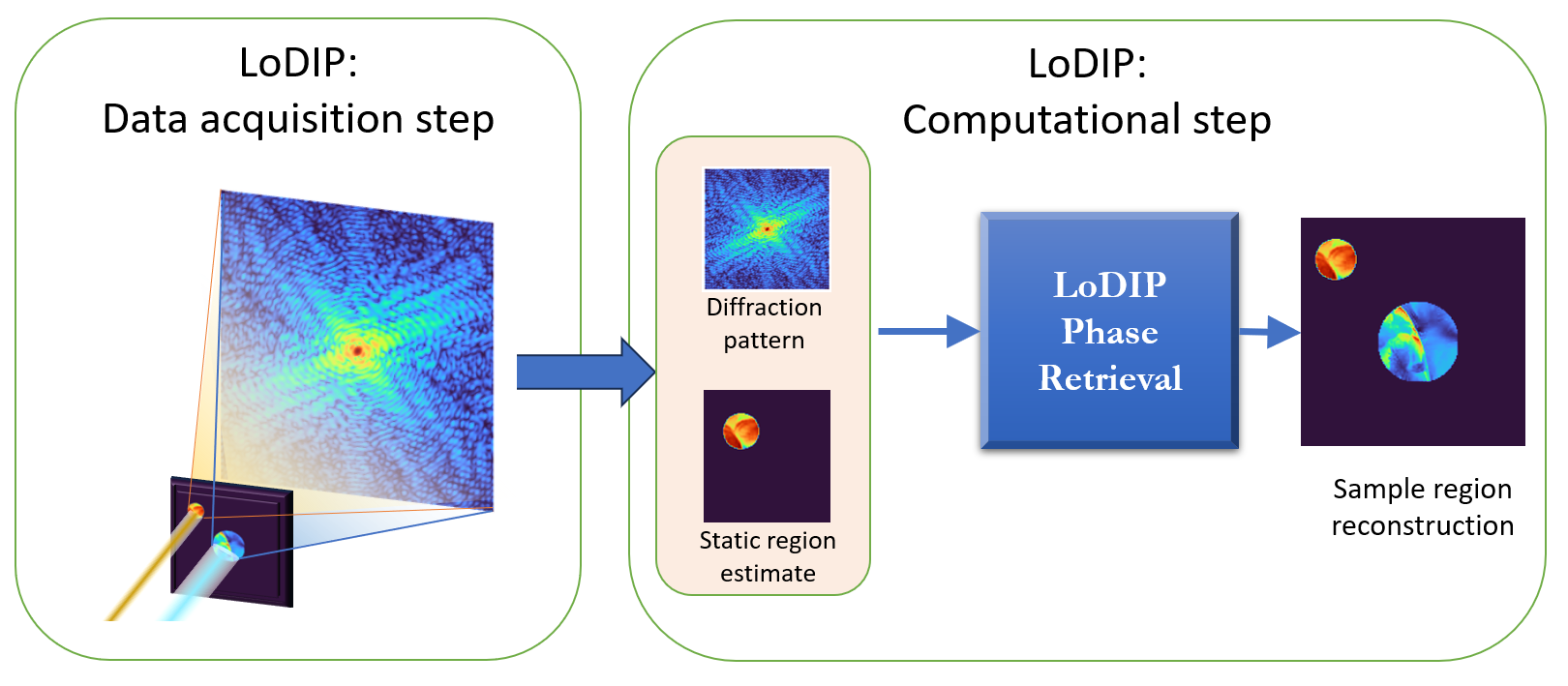
Figure 1: Coherent Diffraction Imaging (CDI) employs a coherent X-ray beam directed at a sample, capturing the resulting diffraction pattern on a 2D detector. A computational algorithm is then applied to reconstruct the desired sample image. Inspired by in-situ CDI [1], LoDIP introduces two modifications to the CDI setup. First, it involves imaging the sample alongside a static region. Secondly, the static region is exposed to a high radiation dose, while the sample’s exposure is significantly reduced through the use of an attenuator. In the computational step, LoDIP takes both the diffraction pattern and an estimated reconstruction of the static region as inputs, generating a sample reconstruction as its output.

Coherent diffractive imaging (CDI) is a lensless imaging technique [2] used for high resolution imaging at nanoscale. CDI has found broad applications across different disciplines due to its remarkable ability to provide high-resolution structural information about a wide range of specimens from biological specimens to nanoscale objects [3].

Unlike visible light, X-rays have high penetrating power and thus can be used to image thick, unfixed specimens. However, many samples of interest for CDI, such as biological material, polymers or organic semiconductors, require minimal radiation exposure to prevent damage during data acquisition [4, 5]. Thus, there is considerable interest in techniques that minimize sample radiation exposure and enable X-ray imaging at extremely low photon counts.

The main challenge is that imaging at low photon counts leads to very high shot noise in the acquired measurements (diffraction pattern) and makes the subsequent image reconstruction (i.e. phase retrieval) very challenging. Under high shot noise, iterative phase retrieval algorithms, including ER, HIO, become unstable, facing challenges such as getting trapped in local minima, stagnation, and failure to converge.

One category of proposed solutions for the low-dose challenge involve modifications to the optical data acquisition setup of CDI [6, 7, 1]. A notable example is in-situ CDI, as introduced by Lo et al. [1] and further explored in [8]. A dose-tolerant static region is positioned next to the sample and is illuminated with a higher radiation dose. This ensures sufficient light reaches the detector while maintaining a low radiation dose on the sample. Multiple measurements are taken over time and the static region is leveraged as a robust time-overlap constraint which regularizes the phase retrieval optimization. However, in order to leverage the time-invariant static region as real-space constraint, this method requires multiple measurements (that is multiple diffraction patterns). Adapting this setup for single-image scenarios results in suboptimal reconstructions (see HIO-stat column in Fig. 4 ).

The solution we propose in this paper is to design a novel data-driven computational algorithm to address single image low-dose phase retrieval. Data-driven approaches have shown potential for simpler versions of phase retrieval at low-photon counts [9, 10], but they cannot be readily adapted to the single-image context due to the requirement for a large training dataset. Deep learning based single-image methods such as deep image prior (DIP) [11, 12] have been used in the past in the single-image context. While they have demonstrated success in simpler phase retrieval scenarios [13, 14, 15], they struggle in low dose situations, as evident from our experiments Fig. 4 and from previous literature on the topic [16, 17].

To address these issues, in this work we propose a deep learning method designed for single-image low-dose phase retrieval. More specifically, we propose LoDIP, a single-image method for low-dose phase retrieval based on DIP and inspired by in-situ CDI. We use the modified imaging setup consisting of a static region illuminated with a high dose of radiation alongside the sample of interest which is illuminated by low-light. This increases the amount of light incident on the detector, without increasing the radiation dose on the sample. Then we modify the DIP framework to exploit the additional constraints coming from this setup. Experiments show that the proposed method LoDIP can reliably work for single-image low-dose phase retrieval both for simulated and experimental data. In particular our experiments show the advantages of LoDIP over state of the art methods: first, being completely data driven, LoDIP does not require specialized algorithmic training to optimize the parameters to obtain satisfactory results. This makes LoDIP accessible to a broad user community. Secondly, our experiments demonstrate that LoDIP outperforms state-of-the-art methods by yielding reconstructions with reduced noise (higher peak signal-to-noise ration) while preserving resolution (comparable Fourier Ring Correlation). Third, since LoDIP is based on the DIP framework, it does not require a large training dataset, in contrast with other deep learning approaches. Finally, being designed for single-image phase retrieval, LoDIP can produce comparable reconstructions to the original in situ CDI method without requiring a time series of measurements.

II Related Work

II-A Coherent Diffractive Imaging

In Coherent Diffractive Imaging (CDI), an object is illuminated by a highly coherent light source. The interaction between the object and the incident wave results in the generation of a diffraction pattern, which is subsequently detected. However, while detectors capture the magnitude of the diffracted wave, the phase information is lost. As a consequence, the process of reconstructing the image of the object of interest necessitates the development of a computational algorithm designed to recover the lost phase from the acquired diffraction pattern. This is commonly referred to as the “phase retrieval” problem. As shown in [18], if the diffraction pattern is sufficiently oversampled, the phase can be retrieved from the diffraction pattern via iterative algorithms (see for instance [19]).

Representing the object of interest by the complex-valued matrix $\mathbf{X}\in\mathbb{C}^{n\times n}$ and the captured diffraction pattern by $\mathbf{Y}\in\mathbb{R}^{m\times m}$, in the conventional phase retrieval configuration the diffraction pattern $\mathbf{Y}$ is obtained through the application of the following forward process:

$$\mathbf{Y}=\left|\mathcal{F}\left(\mathbf{X}\right)\right|^{2}$$ (II.1)

Here, $\mathcal{F}$ represents the Fourier transform, converting the spatial information contained in the object matrix $\mathbf{X}$ into the frequency domain. The magnitude operation $\left|\cdot\right|$ is applied element-wise, capturing the squared amplitude of the transformed frequencies, thus simulating the diffraction pattern resulting from the interaction of an incident wave with the object.

To meet the oversampling criteria, which helps to mitigate the non-uniqueness of the phase retrieval problem, the original object $\mathbf{X}$ is placed in an empty background such that $m=2\times n$. In simulated settings, this oversampling is achieved by zero-padding $\mathbf{X}$ before applying the forward operator. The overall goal of the phase retrieval problem is to recover the image $\mathbf{X}$ from the captured diffraction pattern $\mathbf{Y}$.

Generally, some information about the support of the object (i.e. the location of the object) within the empty background is known. Let $\mathbf{S}_{0}\in\mathbb{C}^{m\times m}$ be the known support information. $S_{0}$ is a matrix containing ones where the object of interest is estimated to be, zeros otherwise. In general one may not know the exact support of the object of interest, but only an estimate of it. This makes the retrieval harder since it leaves some translation freedom (see Fig. 6 for experiments with inaccurate support estimate).

With these assumptions, the phase retrieval problem can be formulated as an optimization problem:

$$\min_{\hat{\mathbf{X}}\in\mathbb{C}^{n\times n}}\;\ell\left(\mathbf{Y},\left|\mathcal{F}\left(\hat{\mathbf{X}}\right)\right|^{2}\right),$$

$$s.t.\left(1-\mathbf{S}_{0}\right)\odot\hat{\mathbf{X}}=[\mathbf{0}]_{m\times m}$$ (II.2)

where the first term imposes that II.1 is satisfied, while the second term is the support constraint. The objective function in the above formulation is referred to as the magnitude constraint or data consistency term. The support constraint imposes that the reconstructed object has the estimated support. We note that the objective function can also be written in terms of the Fourier magnitudes (not squared), i.e. $l(\sqrt{\mathbf{Y}},|\mathcal{F}(\mathbf{X})|)$, this gave similar results in our experiments as the squared case.

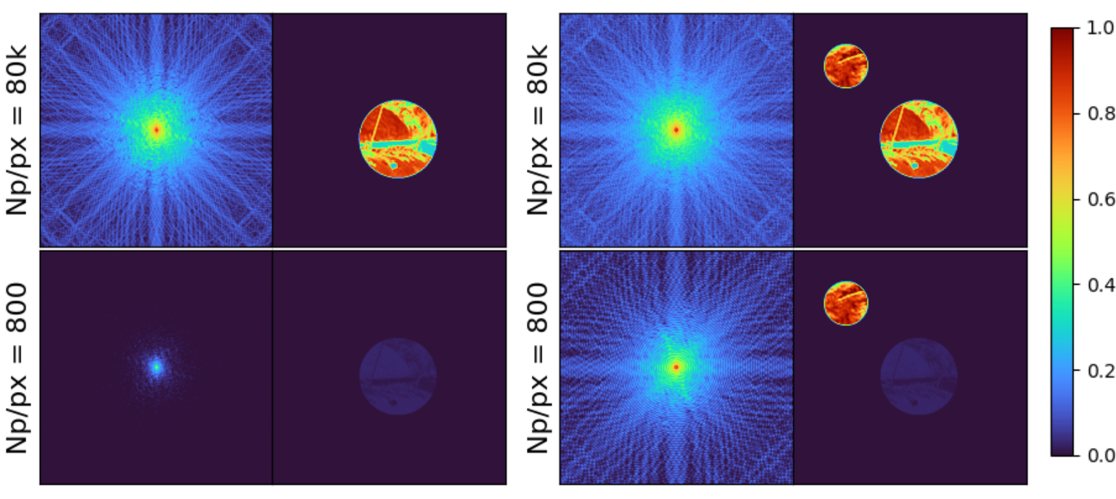
Figure 2: Examples from the simulated data at different levels of illumination of the sample region as measured in photons per pixel (Np/px). [Left] The first two columns are the diffraction pattern and the image sample without a static structure. [Right] And the last two columns are the same sample with a static region. [Top] The first row has a high illumination of 80k Np/px on both the sample and the static region. [Bottom] Whereas the second row has a high illumination of 80k Np/px on the static region and a low illumination of 800 Np/px on the sample. It can be seen that at lower illumination (bottom row), the sample has very low pixel values.

II-B Phase retrieval for low-light imaging

Imaging at cellular or atomic scales necessitates use of X-ray radiation. However, many samples of interest for CDI, such as biological material, polymers or organic semiconductors, require minimal radiation exposure to prevent damage during data acquisition. As a consequence,there is considerable interest in techniques that minimize sample radiation exposure and enable X-ray imaging at extremely low-photon counts. The major challenge of working in the low-dose case is the strong presence of noise in the captured signal. In practice, most of the existing PR methods [20, 21, 22, 23, 24, 25] struggle to work in the low dose setting (high noise). This comes in addition to the existing challenge of working without accurate support information which itself is sufficient for many of the existing algorithms to fail (unless additional strategies are adopted like the shrink-wrap method [26]).

Attempts have been made at low-photon phase retrieval that modify the imaging setup of the problem [6, 7, 1]. While [6] relies on a phase diverse approach, [7, 1] use in the imaging setup a static region made of heavy metals (usually gold) which can withstand high energy light. Among these methods, in-situ CDI [1] achieves a substantial order of magnitude dose reduction over other methods. The main idea is to monitor a dynamic process over time containing two distinct regions: a dynamic area containing the sample which continuously changes, and a static region that remains stationary in time. The static region is subject to significantly higher illumination compared to the sample, ensuring sufficient light falls on the detector, while keeping the radiation dose low for the sample. A series of diffraction patterns is collected over time, resulting in interference between the static and dynamic regions. The static region’s presence in each time step’s measurement offers a strong overlap-in-time constraint for facilitating the convergence of phase retrieval optimization. In the original in situ CDI paper experiments show the reconstruction of the motion of low-dose samples such as glioblastoma cells through Oversampling Smoothness (OSS) algorithm [24].

II-C Deep Learning for phase retrieval

Recent data-driven deep learning methods for phase retrieval [27, 28, 10, 29] have demonstrated that deep neural networks (DNN) within a supervised learning framework can enhance performance in low-light conditions. However, despite some initial successes, deep learning methods for phase retrieval are yet to see widespread adoption among microscopy practitioners. There are a few reasons for why this happens: model training often requires a large dataset, making them unusable in the single-image setting; training often a long time and GPU resources; the reconstruction performance heavily depends on the quality of data provided for the model training. Finally, each model has to be retrained to be used on samples captured under different experimental settings. In this work, we propose a deep learning-based method based on deep image prior which can function in a single-image setting without requiring a large dataset and can be used across datasets and experimental setups.

II-D Neural Networks as a prior

After the success of convolutional neural networks (CNNs) on image classification tasks [30], neural networks and particularly CNNs have improved the state-of-the-art in many computer vision tasks. The majority of these instances were within the framework of supervised learning, requiring the use of extensive datasets for training. More recent works (see for instance [31, 32, 33]) showed that neural networks can succeed in approximating images distribution (this is known as generative modeling). This success led to the use of trained CNNs as a prior for regularizing inverse problems in computer vision [34]. The main idea is to pre-train the model on a similar dataset (possibly for a different task) and use them for inverse problems in a single-sample setting, i.e. without re-training. Around the same time it was discovered that even an untrained neural network can be used as a strong prior for natural images [11, 12] and can be successfully used to regularize inverse problems on natural images.

The surprising success of untrained neural prior or deep image prior (DIP) on inverse problems in image restoration and enhancement has been followed by works aimed at understanding its underlying mechanisms [35]. Subsequent research has resulted in various extensions and adaptations, including approaches involving early stopping strategies [36, 14], methods addressing spectral bias improvements [37], and innovative applications [38]. For a comprehensive overview of the extensive body of work on untrained neural priors in image enhancement, we recommend a recent comprehensive survey [39].

Untrained neural priors have also been applied to computational imaging inverse problems [40, 41, 42] including simpler versions of phase retrieval [13, 14, 15, 43]. However, compared to the setting used in this paper (far-field Fraunhoffer diffraction), these works tackle a much simpler settings for phase retrieval (e.g. near-field Fresnel diffraction).

In this work, we adopt the in-situ CDI setup for the single-image phase retrieval and complement it with an untrained neural network prior in the computational algorithm. Our method is able to produce accurate reconstructions even in the low dose setting, thanks to the in-situ CDI set up and is able to produce results for single-image phase retrieval since the untrained neural network does not require any data. Experiments on simulated and experimental data demonstrate the efficacy of this method over either of these methods alone and other state of the art methods.

III Proposed method

The proposed method, which we refer to as LoDIP, modifies the data acquisition setup of conventional CDI to incorporate a high-dose static region inspired by the in-situ CDI setup. While in-situ CDI leverages the static region as a time-invariant constraint to reconstruct a sequence of dynamic measurements, the high-dose static region serves a different purpose in LoDIP where we are interested in the single-image setting.

Firstly, it increases the available light for image formation on the detector, effectively reducing the impact of shot noise. Additionally, given the high-dose illumination, it is easy to produce an accurate reconstruction of the static region. The known static region is then used as a strong constraint to improve convergence of the phase retrieval optimization. Secondly, it mitigates the ambiguities arising from symmetries in the forward process which is a fundamental difficulty of phase retrieval, (see for instance [19, 44, 45]).

While these adaptations significantly enhance the performance of established phase retrieval methods (such as HIO) at low radiation doses, our experiments (see Fig. 3), show that LoDIP can further improve the final reconstruction quality by incorporating an untrained neural prior for phase retrieval.

III-A LoDIP: Data acquisition

The sample of interest is placed within a finite support next to a static region of heavily scattering, dose-tolerant object such as a gold (Au) pattern on an optical stage. The X-ray illumination on the dose-sensitive sample is reduced to a tolerable limit by the presence of an attenuator, while the static region is exposed to the full dose of the incident illumination. Far-field diffraction patterns recorded from this setup are formed by the interference in Fourier space between the high-dose static region and the sample. These contain Poisson noise relative to the total illumination on the detector. Given the high-dose illumination on the static region and the known support, it is possible to obtain a high-quality static region reconstruction. In this work we use an established iterative method, Generalized Proximal Smoothing (GPS) initialized with 1000 iterations of HIO.

We note explicitly that the placement of the object and the static structure do not influence the reconstruction given by LoDIP, as long as their supports do not overlap. More specifically, let $\mathcal{S}\left(\cdot\right)$ be the operator which extracts the support (location of non-zero elements) of a given image. Then, we assume that the object and the static region have a non-overlapping supports, i.e. $\mathcal{S}\left(\mathbf{X}\right)\odot\mathcal{S}\left(\mathbf{U}\right)=[\mathbf{0}]_{m\times m}$.

III-B LoDIP: Phase Retrieval

For LoDIP, the known static region in the above data acquisition step provides us with a useful constraint to regularize and improve the convergence of the optimization problem. By incorporating the static structure $\mathbf{U}\in\mathbb{C}^{k\times k}$ in the original phase retrieval formulation, the forward process becomes:

$$\mathbf{Y}=\left|\mathcal{F}\left(\mathbf{X}+\mathbf{U}\right)\right|^{2}$$ (III.1)

Here $\mathbf{X}$ and $\mathbf{U}$ are appropriately zero-padded to have the same dimension. In a similar way the optimization problem becomes:

$$\min_{\mathbf{X}\in\mathbb{C}^{n\times n}}\;\ell\left(\mathbf{Y},\left|\mathcal{F}\left(\mathbf{X}+\mathbf{U}\right)\right|^{2}\right),$$

$$s.t.\left(1-\mathbf{S}_{0}\right)\odot\mathbf{X}=[\mathbf{0}]_{m\times m}$$ (III.2)

In LoDIP this setup is further generalized by incorporating the deep image prior framework. In the traditional deep image prior setup, for recovering an image $\mathbf{X}\in\mathbb{C}^{n\times n}$ from its measurements $\mathbf{Y}\in\mathbb{C}^{m\times m}$ the optmization problem is formulated as:

$$\min_{\mathbf{W}}\;\ell\left(\mathbf{Y},\mathcal{A}\left(g_{\mathbf{W}}\left(\mathbf{z}\right)\right)\right),$$ (III.3)

where $\mathbf{Y}=\mathcal{A}\left(\mathbf{X}\right)+\eta$, $\mathcal{A}$ is the known forward operator and $\eta$ is the noise. The optimization variable $\mathbf{X}$ is re-parameterized with a new function $g_{\mathbf{W}}\left(\mathbf{z}\right)$, generally a convolutional neural network. Here $\mathbf{W}$ are the learnable parameters of the network and $\mathbf{z}$ is a random input seed which is fixed throughout the optimization process. In LoDIP we choose $z$ to be the recorded diffraction pattern to provide a strong relation between input and desired output during the optimization process.

More in specifically, we extend the deep image prior setup to incorporate the constraints coming from the above setup: we include the known static region, the known sample support as well as the relative illumination doses on sample and static regions. Since the different doses on the sample and the static region lead to very different range of pixel values for $\mathbf{X}$ and $\mathbf{U}$ we add a scaling factor ($k$) to the optimization objective (Section III-B) to bring the expected output of the neural network to the range $[0,1]$. This greatly improves the final reconstruction quality. Finally the optimization problem solved by LoDIP is:

$$\min_{\mathbf{W}}\;\ell\left(\mathbf{Y},\left|\mathcal{F}\left(k*g_{\mathbf{W}}\left(\mathbf{z}\right)+\mathbf{U}\right)\right|^{2}\right),$$

$$s.t.\left(1-\mathbf{S}_{0}\right)\odot\mathbf{X}=[\mathbf{0}]_{m\times m}$$ (III.4)

Following the literature on this topic, we have used a U-Net [46] with skip connections and ReLU activation functions. The implementation of LoDIP is very flexible and can accommodate multiple modifications. First, any suitable network architecture can be used in the proposed setup. Second, LoDIP can be modified to work in the multiple measurements setting of the original in-situ CDI paper.This interesting modification is left for a future work. Third, LoDIP can seamlessly incorporate a rough reconstruction of the sample as initialization so it can be effectively combined with other techniques designed to generate high-quality initializations for iterative phase retrieval methods [44]. Fourth, LoDIP can be used in the presence of a probe function by incorporating it in the forward operator (this was done in Section IV-B to produce the results for experimental data whose generation required a probe). This makes LoDIP easily adjustable for diverse experimental conditions in contrast to existing state-of-the-art methods such as GPS [25] which would require major modifications to accommodate different experimental setups. Fifth, the performance of LoDIP is not sensitive to the relative size or relative location of the sample and the static structure, nor to the specific choice of the static structure. A static structure design step such as in [45, 47] has the potential to improve the performance, but is not necessary. In fact in our experiments we obtain accurate reconstructions independently of the choice of the static structure (specifically, for each google image reconstruction we use a different static region). Finally, unlike Fourier holography [48, 47], the proposed method works with different illuminations of the sample and the static region.

IV Experimental Results and Discussion

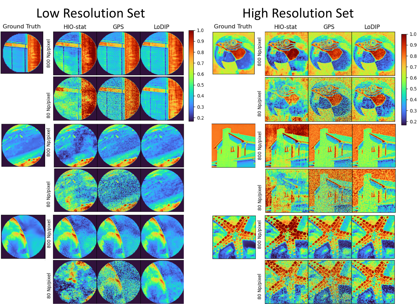
Figure 3: Experimental Results on simulated data. Left: Reconstruction of Low Resolution Set images for 800 Np/pixel (Top rows) and 80 Np/pixel (Bottom rows). Right: Reconstruction of High Resolution Set images for 800 Np/pixel (Top rows) and 80 Np/pixel (Bottom rows). Each image shows a zoomed-in view of only the sample region.

TABLE I: Quantitative comparison of LoDIP and HIO-stat performance. For each metric, the reported values represent the mean over all the samples in the dataset

	Np/px=800			Np/px=80
	Low resolution Set
	PSNR $\uparrow$	SSIM $\uparrow$	$R_{\text{real}}\downarrow$	PSNR $\uparrow$	SSIM $\uparrow$	$R_{\text{real}}\downarrow$
LoDIP	28.52	0.76	0.07	25.09	0.63	0.10
HIO-stat	21.55	0.47	0.18	13.11	0.17	0.44
GPS	22.96	0.53	0.13	13.91	0.29	0.39
	High Resolution Set
LoDIP	23.56	0.59	0.09	20.01	0.42	0.14
HIO-stat	19.90	0.57	0.13	13.99	0.24	0.29
GPS	19.16	0.45	0.15	10.83	0.17	0.40
	Biological cell sample
LoDIP	26.97	0.68	0.11	19.08	0.32	0.26
HIO-stat	21.27	0.50	0.18	12.21	0.14	0.39
GPS	23.68	0.53	0.15	15.14	0.19	0.42

IV-A Data

We perform experiments on three kinds of data. First, we create a simulated data using a procedure similar to [49]. Natural images are used to create the sample region and the static region for each sample in the dataset. Examples of the generated images can be seen in Fig. 2. Next, we create a simulation images of biological cell using physically accurate simulations of a gold lacey for the static structure and a biological cell for the sample region, these can be found in Fig. 4.

Finally, we demonstrate the applicability of LoDIP on experimental diffraction patterns from live glioblastoma cells measured with a 534 nm HeNe laser. The dataset utilized in this study is sourced from the work of Lo et al. [1]. The static structure is a 100 µ pinhole exposed to the same incident illumination as the sample. Unlike the first two datasets above, this data has been collected using a probe. Further information about the generation of simulated data and optical laser data collection can be found in the original paper [1]. .

Experimental setup and data generation

The experimental setup is similar to the one in [1]. The size of the entire image (here, 512x512) corresponds to the size of the detector in the real experimental setup. The support of the sample region is 170x170 pixels. This gives an oversampling ratio of approximately 3.0 which is higher than the theoretical requirement of 2. The sample and the static structure have non-overlapping support and the static structure is set to have half the radius of the sample region (however, the method is independent of the static region size).

Simulating low-light conditions

Based on previous studies on low-dose phase retrieval [1] and [8] on low-dose phase retrieval, the illumination on the sample has been varied from 2.5x$10^{5}$ to 2.5x$10^{9}$ photons per  µm^-2. The illumination on the static structure has been fixed at 2.5x$10^{9}$ photons per  µm^-2. We show results on the low doses of 2.5x$10^{6}$ and 2.5x$10^{7}$ photons per  µm^-2 which corresponds to $800$ and $80$ photons per pixel (Np/px) based on the simulation geometry. This results in different illuminations of the sample and static images. This is clearly seen in Fig. 2, columns two and four, where the sample region becomes darker in the bottom row image, whereas the static image remains the same. Note that as the sample is illuminated by low-dose light, the diffraction pattern is also darker: most of the pixels are close to zero and so Poisson noise is very high in this case.

The illumination in photons per pixel has been calculated by dividing this number of incident photons on the entire sample area by the total number of pixels containing the sample. The lighting conditions have been graded in number of incident photons per pixel (Np/px in Fig. 2). Based on the total number of incident photons, Poisson noise has been applied. Additive white Gaussian noise is commonly used as an approximation for Poisson noise. However, this approximation is only valid at high photon counts. Since in this case we work with low photon counts, we directly sample from the Poisson distribution with mean equal to the number of incident photons on a pixel:

$$N_{p}/px=\frac{\text{\# incident photons}}{\text{\# pixels}}$$ (IV.1)

$$s=\frac{Np}{\sum_{i,j}Y_{i,j}}$$ (IV.2)

$$\mathbf{\tilde{}}{Y}=Poisson(\mathbf{Y}\cdot s)\cdot{\frac{1}{s}}$$ (IV.3)

IV-B Results

For all experiments we compare the relative performance of the proposed method (LoDIP) with other popular methods which can be used in this setup. Specifically, we compare with Hybrid input-output (HIO) [50]; Deep Image Prior [11] (DIP) with no static region information; HIO-stat which is a modification of HIO that uses a static region; and Generalized proximal smoothing (GPS) [25] which is the state of the art method for phase retrieval. HIO and DIP work with diffraction patterns collected without a static region (see column 1 in Fig. 2. Rest of the methods, namely HIO-stat, GPS and LoDIP use the static region, however LoDIP also exploits neural network priors.

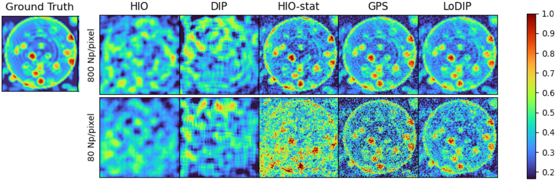
Figure 4: Experimental Results on biological cell sample. (Top row) Reconstruction at 800 Np/pixel. (Bottom row) Reconstruction at 80 Np/pixel).

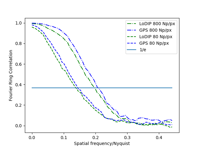
Figure 5: Comparison of FRC values for GPS and LoDIP reconstructions on biological cell at 800 Np/px and 80 Np/px.

Reconstruction of natural images

The proposed method’s robustness and generality are evaluated using natural images. Two commonly used natural image datasets for testing phase retrieval algorithms were selected: the Set12 dataset [51, 52, 53] and internet-sourced stock images used in [49]. For each image, diffraction patterns were first generated using the forward model outlined in Section III and Section IV-A. Results were presented for two low-dose scenarios: 800 and 80 photons per pixel. We observed that the Set12 images exhibited higher resolution and finer details compared to the stock images, thus we refer to these as high and low resolution set respectively. The complementary qualities of the datasets enable a more comprehensive evaluation of each method’s denoising capability and achievable resolution. For each dataset, we compared the reconstructions of each method across 12 samples, with each sample utilizing a different image for its static structure and sample region.

Following previous works on reconstruction with noisy measurements [51], we measure the reconstruction accuracy for all experiments in this paper using using Peak Signal-to-Noise Ratio (PSNR). Higher values of PSNR indicate better fidelity; Structural Similarity Index (SSIM) [53] which measures the similarity between two images, evaluating luminance, contrast, and structure for enhanced accuracy in assessing perceptual image quality. Again higher values indicate better reconstruction; R-factor ($R_{real}$) [25] which measures the degree of agreement between observed and predicted data, commonly used in the assessment of image reconstruction quality. A smaller R-factor indicates a closer agreement between the true and reconstructed image.

The first two rows of Table I show the results for PSNR, SSIM and $R_{real}$ averaged over the entire test set of 12 images for the low and high resolutions sets. Since DIP and HIO without reference regions did not provide good results in this case we omit those methods here. From the table we can see that LoDIP attains better results across all metrics for both data sets and photon counts. The better performance of LoDIP is especially clear in the low photon counts case where LoDIP accuracy is approximately double the accuracy of the other methods. Finally, as expected, the error is higher for the high resolution set as more fine detail has to be reconstructed.

Fig. 3 displays a comparison of the results of LoDIP, HIO with static structure and GPS for images in the low resolution set (left) and high resolution set (right). To study the robustness of our method with respect to the experimental setup we used a circular mask for low resolution set and a square one for the high resolution set. From this figure we can clearly see that GPS and LoDIP produce the best results (as already shown by the metrics in the table), but that GPS produces images that are more noisy than LoDIP reconstructions, showing that LoDIP has a strong denoising ability. The figure shows also the choice of the mask for the sample region does not influence the reconstruction quality for LoDIP (and for the other methods).

We also note that iterative methods such as HIO-stat and GPS require parameter tuning by experts in the field and often multiple independent runs of the algorithm are necessary to obtain good reconstruction. On the other hand, LoDIP hyper-parameter tuning is minimal and convergence is usually obtained in one run. These experiments show that LoDIP is able to provide accurate and denoised reconstructions for both photon counts while preserving the resolution obtained by state of the art iterative method like GPS.

Reconstruction of biological cell sample

Computational microscopy represents a major potential application of the proposed method. Following previous works on PR for CDI [1, 8], we evaluated the performance of LoDIP on realistic and physically accurate simulated data for a prototypical live cell. , The static structure and biological cell were simulated as done in [1]. The results in this section use a simulated 20-nm thick gold lacey pattern as the static structure and a simulated cell consisting of a vesicle containing water and protein aggregates.

Fig. 4 shows the reconstructions from the same HIO, DIP, HIO with static region, LoDIP and GPS at both doses (respectively 800 and 80 photons/pixel). The static region is unknown and estimated using the procedure described in Section III-A. Similar to the case of natural images, GPS and LoDIP produce the best reconstructions in both cases with LoDIP providing a less noisy reconstructed image than GPS especially in the low photon counts case. HIO and DIP without reference regions fail in the reconstruction. The last row of Table I show the results for PSNR, SSIM and $R_{real}$ in the low photons counts case. Again LoDIP outperforms the other methods across all metrics.

FRC is a technique used in microscopy [1, 8] to assess the resolution and overall quality of a reconstruction: it calculates the correlation coefficient between the Fourier transforms of two images, measured within concentric rings of varying spatial frequencies. The resolution is assessed based on the drop in correlation at high frequencies, with a threshold of 0.367 (for more details see [54]). Higher FRC values correspond to better resolution. Fig. 5 displays the Fourier Ring Correlation (FRC) for both photon counts cases for LoDIP and GPS. The resolution of the reconstruction obtained by LoDIP is comparable to the one obtained by GPS. This indicates that the denoising capability of LoDIP results in only a minimal loss of fine-scale details.

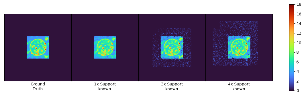
Figure 6: Reconstruction using LoDIP at 80 Np/px without knowledge of accurate support. The columns from left to right are (1) The ground truth, (2) reconstruction with knowledge of the exact support (PSNR=20.08), (3) reconstruction with an approximate support of 3x the actual size (PSNR=20.06), (4) 4x the actual size (PSNR=19.85). Both visually and quantitatively, the LoDIP reconstruction is robust to inaccurate specification of the support. PSNR is calculated only over the exact sample region.

In practice, image reconstruction without precise support information presents a common and challenging problem. To conclude this section, we investigate the robustness of the proposed LoDIP method when dealing with only approximately known support for the biological cell example in the low photons count case.

In Fig. 6, the second column shows reconstruction at 80 Np/px when accurate size and shape of the support is known. The last two columns show the reconstruction when the size of the known support estimate is 3 times and 4 times the size of the actual support. From these results we can see that LoDIP reconstructions are robust to inaccurate support specification. Widely used phase retrieval algorithms struggle when accurate support information is not available [43, 26]. This can be partially mitigated by employing heuristic subroutine such as shrinkwrap [26] to refine the support estimate every few iterations. While effective, these end up increasing the total number of hyperparameters needed to be tuned. LoDIP does not require any such subroutine for support estimation.

Reconstruction from experimental data

Finally, we perform an experiment to demonstrate the proposed method on experimentally captured diffraction patterns (one of them is shown in Fig. 7 left column). Unlike the previous experiments, the object is complex-valued and the optical setup includes a probe. The data for this section is the one provided in [1]. We note explicitly that in this dataset the static and sample images have the same high dose, so this is not exactly the setup for which our method is designed. In fact, our method is especially advantageous in the low dose setting, as the previous experiments show, while it obtains comparable results as other methods in the high dose setting. Nonetheless, this setup is very close to the one of interest so we included it in this work. Generating a new experimental dataset with different doses on the static and sample images is left for a future work.

The original in-situ CDI method [1] uses 50 diffraction patterns with a fixed time-invariant static structure required in all the images. HIO-stat and LoDIP use only a single diffraction pattern and perform single-instance phase retrieval. This is an advantage over in situ CDI since as in many experimental setups a truly static structure is difficult to ensure because of the data collection procedure (e.g. in collecting tomographic data, which requires shifting or tilting both the sample and the static structure). In this section, the reconstruction given by in situ CDI is used as a proxy for the ground truth. In fact, a comparison between in situ CDI and LoDIP would be unfair since LoDIP uses 50 times less data (only one diffraction pattern instead of 50). A comparison with GPS is not possible for this data since the current version of GPS does not support Fresnel propagation and adding this would require major modifications which are outside of the scope of this work. In these experiments, LoDIP and HIO-stat have been modified to incorporate the known probe function.

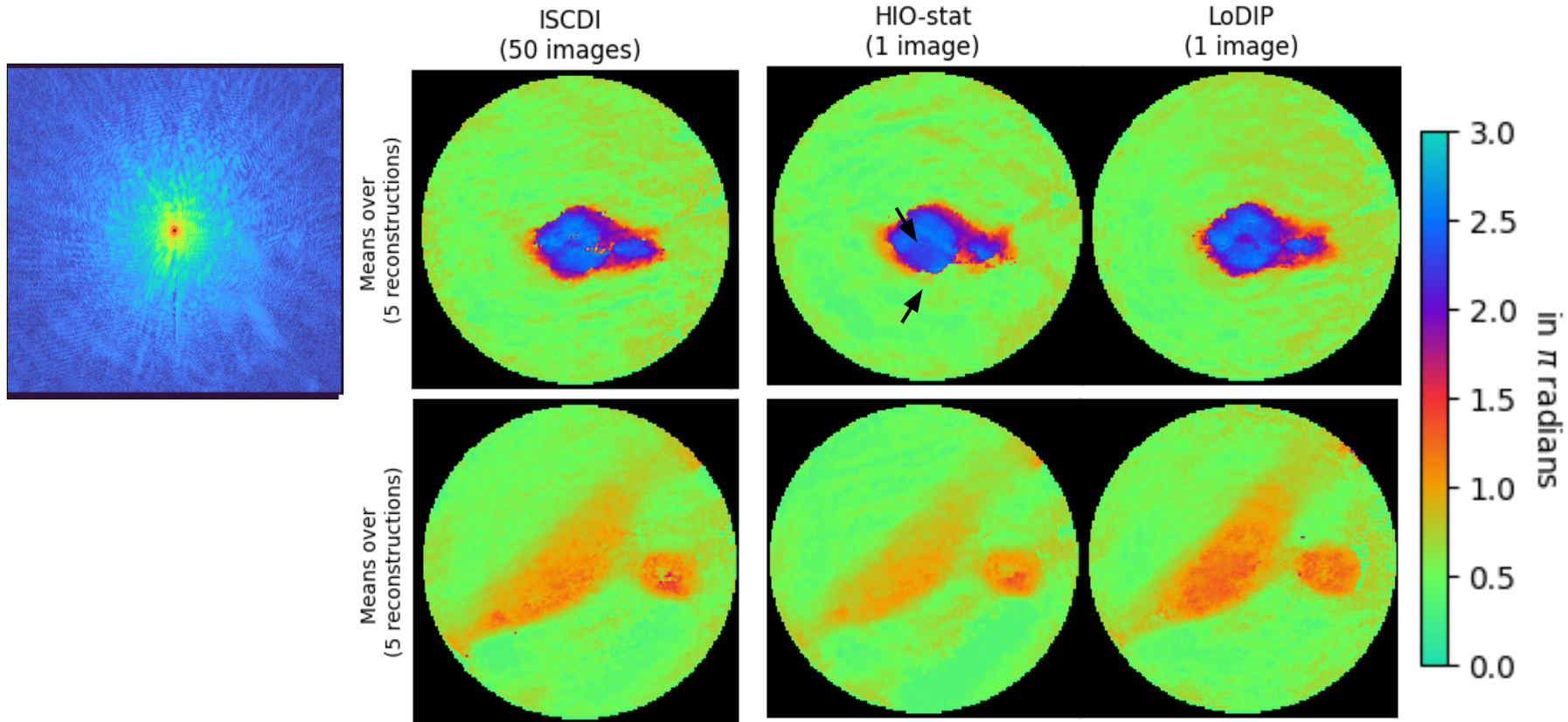
Figure 7: Reconstruction of experimental data (Left) Experimentally captured diffraction pattern. (Right) Reconstruction from different methods.The mean of the top five reconstructions from 20 independent runs is shown in the figure. The static and sample images in this example have the same high dose. LoDIP is especially advantageous in the low dose setting, as the previous experiments show, so as expected, in this high dose setting LoDIP obtains comparable results as in situ CDI and HIO in terms of $R_{F}$. However, LoDIP uses a single diffraction pattern to produce a reconstruction of comparable quality as in-situ CDI which uses 50 samples. Moreover, while HIO-stat reconstruction has similar $R_{F}$ as LoDIP, it contains visible artefacts (indicated by the arrows).

Since there is no ground truth available, to evaluate our results we use R-factor in the Fourier domain. This measures the disagreement between the captured diffraction pattern $\mathbf{Y}$ to the Fourier magnitudes $\lvert\mathcal{F}\left(\hat{\mathbf{X}}\right)\rvert$ of the reconstruction $\hat{\mathbf{X}}$ and is defined as:

$$R_{F}(\hat{\mathbf{X}})=\frac{\sum_{i,j}\left|\lvert\mathcal{F}\left(\hat{\mathbf{X}}\right)\rvert_{i,j}-\mathbf{Y}_{i,j}\right|}{\sum_{i,j}Y_{i,j}}$$ (IV.4)

The reconstruction obtained through in situ CDI yields an R-factor of $30.22\%(\pm 0.97\%)$. As explained before in situ CDI utilizes 50 diffraction patterns for its reconstruction. Comparing this R-factor directly with LoDIP, which only uses a single diffraction pattern, would be unfair due to the substantial difference in data quantity needed to obtain the reconstruction. However, we can use in situ CDI R-factor as a benchmark to assess the performance of our method. The average $R_{F}$ from 20 independent reconstructions based on a single diffraction pattern using both LoDIP and HIO-stat is presented in Table II. Remarkably, LoDIP achieves a comparable R-factor to in-situ CDI, highlighting its efficacy even without the need for multiple diffraction patterns, making it less data-intensive. Interestingly, HIO-stat also demonstrates a comparable R-factor to LoDIP in this scenario. It’s important to note, however, that this success is primarily attributed to the high photon count setting of this experiment, where many methods perform well. It is crucial also to note that, as demonstrated in previous experiments, HIO-stat’s performance diminishes in low photon count settings, providing less accurate results than LoDIP in this more realistic case. Finally, Fig. 7 shows the averaged top 5 reconstructions out of 20 independent runs for all methods. We see that HIO-stat introduces visible artifacts in its reconstruction while LoDIP does not (again the in situ CDI reconstruction is treated as a proxy for the ground truth in this case). Therefore, these results highlight the robustness and adaptability of LoDIP, showcasing its ability to easily accommodate changes in the data acquisition setup and maintain reliable reconstructions across varying experimental conditions.

TABLE II: Quantitative comparison on experimental data. The mean and standard deviation of R-factor($R_{F}$) values are calculated over 20 independent reconstructions each of 5 different samples.

	$R_{F}$
HIO-stat	34.70%($\pm$0.03%)
LoDIP	33.20%($\pm$0.03%)

V Conclusion and Future Work

Emerging deep learning methods present several opportunities to improve upon and expand the scope of computational imaging techniques that require processing steps framed as mathematical optimization problems. The LoDIP approach, introduced in this work, integrates the optimization framework of untrained neural network priors with a precise forward model inspired by the in-situ CDI setup. This combination aims to recover sample images from measured far-field diffraction patterns, particularly in situations where well-established iterative algorithms struggle to achieve proper convergence. We have demonstrated that LoDIP yields an improvement in reconstruction across multiple metrics and samples, especially under low-dose conditions. Moreover, it does not require labeled training data, complex tuning of hyper-parameters, or supervision from a specialist in phase retrieval algorithms. We tested LoDIP for multiple samples and static regions including synthetic data generated from google images, realistic biological cells and experimental data with known and unknown static regions. Our experiments demonstrate LoDIP’s versatility, showcasing its successful application to a wide variety of samples. Furthermore, we showed that LoDIP outperforms state-of-the-art methods in obtaining a denoised reconstructed image, while preserving resolution. We anticipate applications of the LoDIP method to X-ray imaging of dose-sensitive samples of importance in a variety of fields, such as organic semiconductors relevant to modern perovskite solar cells and battery materials, as well as biological samples concerning cellular interactions and life cycles.

References

- [1] Y. H. Lo, L. Zhao, M. Gallagher-Jones, A. Rana, J. J. Lodico, W. Xiao, B. Regan, and J. Miao, “In situ coherent diffractive imaging,” Nature communications, vol. 9, no. 1, p. 1826, 2018.
- [2] J. Miao, P. Charalambous, J. Kirz, and D. Sayre, “Extending the methodology of x-ray crystallography to allow imaging of micrometre-sized non-crystalline specimens,” Nature, vol. 400, no. 6742, pp. 342–344, 1999.
- [3] J. Miao, T. Ishikawa, I. K. Robinson, and M. M. Murnane, “Beyond crystallography: Diffractive imaging using coherent x-ray light sources,” Science, vol. 348, no. 6234, pp. 530–535, 2015.
- [4] G. N. George, I. J. Pickering, M. J. Pushie, K. Nienaber, M. J. Hackett, I. Ascone, B. Hedman, K. O. Hodgson, J. B. Aitken, A. Levina, C. Glover, and P. A. Lay, “X-ray-induced photo-chemistry and X-ray absorption spectroscopy of biological samples,” Journal of Synchrotron Radiation, vol. 19, no. 6, pp. 875–886, Nov 2012. [Online]. Available: https://doi.org/10.1107/S090904951203943X
- [5] E. F. Garman and M. Weik, “X-ray radiation damage to biological macromolecules: further insights,” Journal of Synchrotron Radiation, vol. 24, no. 1, pp. 1–6, Jan 2017. [Online]. Available: https://doi.org/10.1107/S160057751602018X
- [6] C. T. Putkunz, J. N. Clark, D. J. Vine, G. J. Williams, M. A. Pfeifer, E. Balaur, I. McNulty, K. A. Nugent, and A. G. Peele, “Phase-diverse coherent diffractive imaging: High sensitivity with low dose,” Physical review letters, vol. 106, no. 1, p. 013903, 2011.
- [7] T.-Y. Lan, P.-N. Li, and T.-K. Lee, “Method to enhance the resolution of x-ray coherent diffraction imaging for non-crystalline bio-samples,” New Journal of Physics, vol. 16, no. 3, p. 033016, 2014.
- [8] X. Lu, M. Pham, E. Negrini, D. Davis, S. J. Osher, and J. Miao, “Computational microscopy beyond perfect lenses,” arXiv preprint arXiv:2306.11283, 2023.
- [9] A. Goy, K. Arthur, S. Li, and G. Barbastathis, “Low photon count phase retrieval using deep learning,” Physical review letters, vol. 121, no. 24, p. 243902, 2018.
- [10] M. Deng, S. Li, A. Goy, I. Kang, and G. Barbastathis, “Learning to synthesize: robust phase retrieval at low photon counts,” Light: Science & Applications, vol. 9, no. 1, p. 36, 2020.
- [11] D. Ulyanov, A. Vedaldi, and V. Lempitsky, “Deep image prior,” in Proceedings of the IEEE conference on computer vision and pattern recognition, 2018, pp. 9446–9454.
- [12] U. Dmitry, A. Vedaldi, and L. Victor, “Deep image prior,” International Journal of Computer Vision, vol. 128, no. 7, pp. 1867–1888, 2020.
- [13] F. Wang, Y. Bian, H. Wang, M. Lyu, G. Pedrini, W. Osten, G. Barbastathis, and G. Situ, “Phase imaging with an untrained neural network,” Light: Science & Applications, vol. 9, no. 1, p. 77, 2020.
- [14] R. Heckel and P. Hand, “Deep decoder: Concise image representations from untrained non-convolutional networks,” arXiv preprint arXiv:1810.03982, 2018.
- [15] E. Bostan, R. Heckel, M. Chen, M. Kellman, and L. Waller, “Deep phase decoder: self-calibrating phase microscopy with an untrained deep neural network,” Optica, vol. 7, no. 6, pp. 559–562, 2020.
- [16] K. Tayal, C.-H. Lai, V. Kumar, and J. Sun, “Inverse problems, deep learning, and symmetry breaking,” arXiv preprint arXiv:2003.09077, 2020.
- [17] Z. Zhuang, D. Yang, F. Hofmann, D. Barmherzig, and J. Sun, “Practical phase retrieval using double deep image priors,” arXiv:2211.00799, 2022.
- [18] J. Miao, D. Sayre, and H. Chapman, “Phase retrieval from the magnitude of the fourier transforms of nonperiodic objects,” JOSA A, vol. 15, no. 6, pp. 1662–1669, 1998.
- [19] Y. Shechtman, Y. C. Eldar, O. Cohen, H. N. Chapman, J. Miao, and M. Segev, “Phase retrieval with application to optical imaging: A contemporary overview,” IEEE Signal Processing Magazine, vol. 32, no. 3, pp. 87–109, may 2015.
- [20] J. R. Fienup, “Reconstruction of an object from the modulus of its fourier transform,” Optics letters, vol. 3, no. 1, pp. 27–29, 1978.
- [21] J. Miao, J. Kirz, and D. Sayre, “The oversampling phasing method,” Acta Crystallographica Section D: Biological Crystallography, vol. 56, no. 10, pp. 1312–1315, 2000.
- [22] H. H. Bauschke, P. L. Combettes, and D. R. Luke, “Phase retrieval, error reduction algorithm, and fienup variants: a view from convex optimization,” Journal of the Optical Society of America A, vol. 19, no. 7, p. 1334, jul 2002.
- [23] D. R. Luke, “Relaxed averaged alternating reflections for diffraction imaging,” Inverse problems, vol. 21, no. 1, p. 37, 2004.
- [24] J. A. Rodriguez, R. Xu, C.-C. Chen, Y. Zou, and J. Miao, “Oversampling smoothness: an effective algorithm for phase retrieval of noisy diffraction intensities,” Journal of applied crystallography, vol. 46, no. 2, pp. 312–318, 2013.
- [25] M. Pham, P. Yin, A. Rana, S. Osher, and J. Miao, “Generalized proximal smoothing (gps) for phase retrieval,” Optics Express, vol. 27, no. 3, pp. 2792–2808, 2019.
- [26] S. Marchesini, H. He, H. N. Chapman, S. P. Hau-Riege, A. Noy, M. R. Howells, U. Weierstall, and J. C. Spence, “X-ray image reconstruction from a diffraction pattern alone,” Physical Review B, vol. 68, no. 14, p. 140101, 2003.
- [27] A. Sinha, J. Lee, S. Li, and G. Barbastathis, “Lensless computational imaging through deep learning,” Optica, vol. 4, no. 9, p. 1117, sep 2017.
- [28] A. Goy, K. Arthur, S. Li, and G. Barbastathis, “Low photon count phase retrieval using deep learning,” Physical Review Letters, vol. 121, no. 24, dec 2018.
- [29] T. Uelwer, A. Oberstraß, and S. Harmeling, “Phase retrieval using conditional generative adversarial networks,” arXiv:1912.04981, 2019.
- [30] A. Krizhevsky, I. Sutskever, and G. E. Hinton, “Imagenet classification with deep convolutional neural networks,” Communications of the ACM, vol. 60, no. 6, pp. 84–90, 2017.
- [31] D. P. Kingma and M. Welling, “Auto-encoding variational bayes,” arXiv preprint arXiv:1312.6114, 2013.
- [32] I. Goodfellow, J. Pouget-Abadie, M. Mirza, B. Xu, D. Warde-Farley, S. Ozair, A. Courville, and Y. Bengio, “Generative adversarial networks,” Communications of the ACM, vol. 63, no. 11, pp. 139–144, 2020.
- [33] D. P. Kingma and P. Dhariwal, “Glow: Generative flow with invertible 1x1 convolutions,” Advances in neural information processing systems, vol. 31, 2018.
- [34] A. Bora, A. Jalal, E. Price, and A. G. Dimakis, “Compressed sensing using generative models,” in International Conference on Machine Learning. PMLR, 2017, pp. 537–546.
- [35] Z. Cheng, M. Gadelha, S. Maji, and D. Sheldon, “A bayesian perspective on the deep image prior,” in Proceedings of the IEEE/CVF Conference on Computer Vision and Pattern Recognition, 2019, pp. 5443–5451.
- [36] H. Wang, T. Li, Z. Zhuang, T. Chen, H. Liang, and J. Sun, “Early stopping for deep image prior,” arXiv preprint arXiv:2112.06074, 2021.
- [37] Z. Shi, P. Mettes, S. Maji, and C. G. Snoek, “On measuring and controlling the spectral bias of the deep image prior,” International Journal of Computer Vision, vol. 130, no. 4, pp. 885–908, 2022.
- [38] Y. Gandelsman, A. Shocher, and M. Irani, “” double-dip”: unsupervised image decomposition via coupled deep-image-priors,” in Proceedings of the IEEE/CVF Conference on Computer Vision and Pattern Recognition, 2019, pp. 11 026–11 035.
- [39] Y. Lu, Y. Lin, H. Wu, Y. Luo, X. Zheng, and L. Wang, “All one needs to know about priors for deep image restoration and enhancement: A survey,” arXiv preprint arXiv:2206.02070, 2022.
- [40] M. Z. Darestani and R. Heckel, “Accelerated mri with un-trained neural networks,” IEEE Transactions on Computational Imaging, vol. 7, pp. 724–733, 2021.
- [41] A. Qayyum, I. Ilahi, F. Shamshad, F. Boussaid, M. Bennamoun, and J. Qadir, “Untrained neural network priors for inverse imaging problems: A survey,” IEEE Transactions on Pattern Analysis and Machine Intelligence, 2022.
- [42] G. Ongie, A. Jalal, C. A. M. R. G. Baraniuk, A. G. Dimakis, and R. Willett, “Deep learning techniques for inverse problems in imaging,” IEEE Journal on Selected Areas in Information Theory, 2020.
- [43] K. Tayal, R. Manekar, Z. Zhuang, D. Yang, V. Kumar, F. Hofmann, and J. Sun, “Phase retrieval using single-instance deep generative prior,” in Applied Industrial Spectroscopy. Optica Publishing Group, 2021, pp. JW2A–37.
- [44] R. Manekar, Z. Zhuang, K. Tayal, V. Kumar, and J. Sun, “Deep learning initialized phase retrieval,” in NeurIPS 2020 Workshop on Deep Learning and Inverse Problems, 2020.
- [45] R. Hyder, Z. Cai, and M. S. Asif, “Solving phase retrieval with a learned reference,” in Computer Vision–ECCV 2020: 16th European Conference, Glasgow, UK, August 23–28, 2020, Proceedings, Part XXX 16. Springer, 2020, pp. 425–441.
- [46] O. Ronneberger, P. Fischer, and T. Brox, “U-net: Convolutional networks for biomedical image segmentation,” in International Conference on Medical image computing and computer-assisted intervention. Springer, 2015, pp. 234–241.
- [47] D. A. Barmherzig, J. Sun, P.-N. Li, T. J. Lane, and E. J. Candes, “Holographic phase retrieval and reference design,” Inverse Problems, vol. 35, no. 9, p. 094001, 2019.
- [48] I. McNulty, J. Kirz, C. Jacobsen, E. H. Anderson, M. R. Howells, and D. P. Kern, “High-resolution imaging by fourier transform x-ray holography,” Science, vol. 256, no. 5059, pp. 1009–1012, 1992.
- [49] D. J. Chang, C. M. O’Leary, C. Su, D. A. Jacobs, S. Kahn, A. Zettl, J. Ciston, P. Ercius, and J. Miao, “Deep-learning electron diffractive imaging,” Physical review letters, vol. 130, no. 1, p. 016101, 2023.
- [50] J. R. Fienup, “Phase retrieval algorithms: a comparison,” Applied Optics, vol. 21, no. 15, p. 2758, aug 1982.
- [51] C. A. Metzler, P. Schniter, A. Veeraraghavan, and R. G. Baraniuk, “prdeep: Robust phase retrieval with a flexible deep network,” arXiv preprint arXiv:1803.00212, 2018.
- [52] K. Zhang, W. Zuo, Y. Chen, D. Meng, and L. Zhang, “Beyond a gaussian denoiser: Residual learning of deep cnn for image denoising,” IEEE transactions on image processing, vol. 26, no. 7, pp. 3142–3155, 2017.
- [53] H. Lawrence, D. A. Barmherzig, M. Eickenberg, and M. Gabrie, “Low-photon holographic phase retrieval via a deep decoder neural network,” in Optical Sensors. Optica Publishing Group, 2021, pp. JTu5A–19.
- [54] M. van Heel and M. Schatz, “Fourier shell correlation threshold criteria,” Journal of Structural Biology, vol. 151, no. 3, pp. 250–262, 2005. [Online]. Available: https://www.sciencedirect.com/science/article/pii/S1047847705001292