Observation of the $\PGXmb\to\PGyP{2S}\PGXm$ decay and studies of the $\PGXstzb$ baryon in proton-proton collisions at $\sqrt{s}=13\TeV$

Abstract

The first observation of the decay $\PGXmb\to\PGyP{2S}\PGXm$ and measurement of the branching ratio of $\PGXmb\to\PGyP{2S}\PGXm$ to $\PGXmb\to\PJGy\PGXm$ are presented. The $\PJGy$ and $\PGyP{2S}$ mesons are reconstructed using their dimuon decay modes. The results are based on proton-proton colliding beam data from the LHC collected by the CMS experiment at $\sqrt{s}=13\TeV$ in 2016–2018, corresponding to an integrated luminosity of 140. The branching fraction ratio is measured to be $\mathcal{B}(\PGXmb\to\PGyP{2S}\PGXm)/\mathcal{B}(\PGXmb\to\PJGy\PGXm)=0.84^{+0.21}_{-0.19}\stat\pm 0.10\syst\pm 0.02\,(\mathcal{B})$, where the last uncertainty comes from the uncertainties in the branching fractions of the charmonium states. New measurements of the $\PGXstzb$ baryon mass and natural width are also presented, using the $\PGXmb\PGpp$ final state, where the $\PGXmb$ baryon is reconstructed through the decays $\PJGy\PGXm$, $\PGyP{2S}\PGXm$, $\PJGy\PGL\PKm$, and $\PJGy\PGSz\PKm$. Finally, the fraction of the $\PGXmb$ baryons produced from $\PGXstzb$ decays is determined.

0.1 Introduction

The $\PGXb$ family consists of baryons that form isodoublets composed of a triplet of , , and quarks, where corresponds to a or quark for the $\PGXzb$ and $\PGXmb$ states, respectively. Three such isodoublets that are neither orbitally nor radially excited should exist [Th:diquark]. These include one with the spin of the light diquark $j_{\PQq\PQs}=0$ and spin-parity of the baryon $J^{P}=1/2^{+}$ ($\PGXb$ ground states), one with $j_{\PQq\PQs}=1$ and $J^{P}=1/2^{+}$ ($\PGXprb$), and another with $j_{\PQq\PQs}=1$ and $J^{P}=3/2^{+}$ ($\PGXstb$). The ground states were discovered more than a decade ago at the Fermilab Tevatron [XibD0, XibCDF, Xib0CDF] via their decays to $\PJGy\PGXm$ and $\PGXpc\PGpm$. Three of the four states with $j_{\PQq\PQs}=1$ have been observed during the last decade at the CERN LHC [BPH12001, LHCb_XibStar0, LHCb_XibPrime-Star-] via their $\PGXmb\PGpp$ and $\PGXzb\PGpm$ decays, as expected from theoretical predictions [Th:b_bar_1/Nc, Th:b_baryons, Th:m_bb_rel_quark_model]. The fourth state, $\PGXprzb$, is expected to have a mass lower than the $\PGXmb\PGpp$ mass threshold, making a strong decay to the $\PGXmb$ baryon kinematically impossible. Several other more massive $\PGXb$ resonances were also observed recently by the CMS and LHCb Collaborations [LHCb_Xib6227, LHCb_Xib6227_2020, BPH20004, LHCb_Xib_1D, LHCb_Xbss] via their decays to $\PGXzb\PGpm$, $\PGXmb\PGpp$, $\PGXmb\PGpp\PGpm$, $\PGXzb\PGpp\PGpm$, $\PGLzb\PKm$, and $\PGLzb\PKm\PGpp$. Various theoretical models and calculations predict a spectrum of excited $\PGXb$ baryons [Th:m_bb_rel_quark_model, Th:b_bar_1/Nc, Th:b_baryons, Th:bb_in_quark_model, Th:regge_bb_rel, Th:faddeev_bb_spectr, Th:LQ_XQ_heavy_quark, Th:ITEP_Trusov, Th:sum_rule_Pwave, Th:12_32_heavy, Th:S_P_waves_single_bb, Th:heavy_w_chiral, Th:bb_hyperfine, Th:regge_traj, Th:spectr_123_bb], and the observed resonances are considered to be $1P$ isodoublets of $\PGXb$ or $\PGXprb$ states, and a $1D$ doublet. However, larger data samples are needed to measure the quantum numbers of these resonances. There is also the possibility that some of the observed wide resonances could instead be unresolved overlapping narrow states.

Besides the searches for excited $\PGXb$ states, the LHCb Collaboration has observed new ground-state $\PGXb$ decays and determined some of their branching fractions [LHCb_Xb_Dph_Lch, LHCb_Xb_Lbpi, LHCb_Xbdec_pKK, LHCb_JpsiLamK, LHCb_Xb_charmless, LHCb_Xb_JpsiV0]. The spectrum of excited $\PGXb$ baryons can be classified relatively easily, especially with the guidance of the similar and well-established baryons [PDG]. By contrast, the wide variety of decay modes available in the weak decay of the ground-state baryons presents a significant theoretical challenge, and predictions of the branching fractions to various final states are less straightforward. Multibody decays of $\PGXb$ baryons can contain rich resonant structures, including both conventional and exotic resonances, such as excited $\PGXm$ states and the $P^{\PGL}_{\PGy\PQs}(4459)^{0}$ pentaquark reported in the $\PGXmb\to\PJGy\PGL\PKm$ decay [LHCb_JpsiLamK_2020]. The search for new $\PGXb$ decays is also important in the quest for observing possible $CP$ violation [LHCb_Xbdec_pKK_CP]. In general, both weak decays of heavy baryons and their strongly decaying excitations can be described in the framework of heavy-quark effective theory (HQET) [Th:HQET, Th:hq_spectr_sym, Th:weak_decay_itep, Th:weak_decay_heavy, Th:hqet_nonper]. Measurements of the decays and properties of both ground and excited $\PGXb$ states provide coherent and complementary input to HQET, which could improve our understanding of the quantum chromodynamic (QCD) mechanisms responsible for quark dynamics and the formation of hadrons.

In this paper, we study $\PGXmb$ and $\PGXstzb$ baryon states using a sample of proton-proton (pp) collisions from the LHC, collected by the CMS experiment in 2016–2018 at $\sqrt{s}=13\TeV$, corresponding to an integrated luminosity of 140 [Sirunyan:2759951, CMS-PAS-LUM-17-004, CMS-PAS-LUM-18-002]. The inclusion of charge-conjugate states is implied throughout this paper, unless otherwise noted. We report the first observation of the $\PGXmb\to\PGyP{2S}\PGXm$ decay and the measurement of its branching fraction with respect to the well-known $\PGXmb\to\PJGy\PGXm$ decay. In both signal and normalization channels, the charmonium states are reconstructed through their dimuon decay modes, and $\PGXm$ decays to $\PGL\PGpm$ with the following $\PGL\to\Pp\PGpm$ are used. Thus, the relative branching ratio $R$ is measured using the following expression:

$$R=\dfrac{\mathcal{B}(\PGXmb\to\PGyP{2S}\PGXm)}{\mathcal{B}(\PGXmb\to\PJGy\PGXm)}=\dfrac{N(\PGXmb\to\PGyP{2S}\PGXm)}{N(\PGXmb\to\PJGy\PGXm)}\dfrac{\epsilon(\PGXmb\to\PJGy\PGXm)}{\epsilon(\PGXmb\to\PGyP{2S}\PGXm)}\,\dfrac{\mathcal{B}(\PJGy\to\PGmp\PGmm)}{\mathcal{B}(\PGyP{2S}\to\PGmp\PGmm)},$$ (1)

where $N$ and $\epsilon$ represent the measured number of signal events in data and the total efficiency from Monte Carlo (MC) simulation, respectively, for each of the respective decay modes. The values of the branching fractions $\mathcal{B}$ in the last term are taken from the PDG [PDG]. Even though the value of $\mathcal{B}(\PGXmb\to\PJGy\PGXm)$ is not known, the choice of this normalization channel is quite natural since it has the same topology and similar kinematic properties as the signal channel, reducing the systematic uncertainty in the ratio related to the reconstruction of the muons and the other charged particle tracks from the $\PGXmb$ decays.

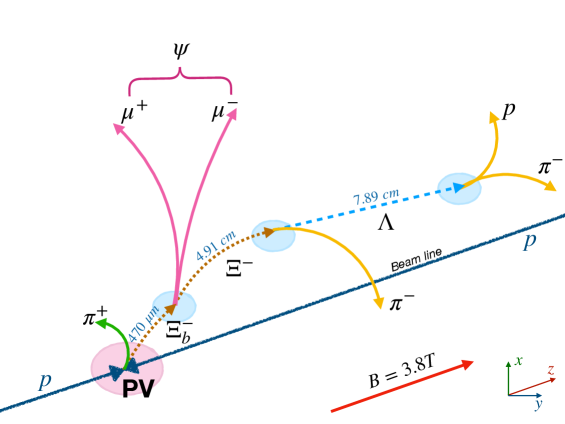
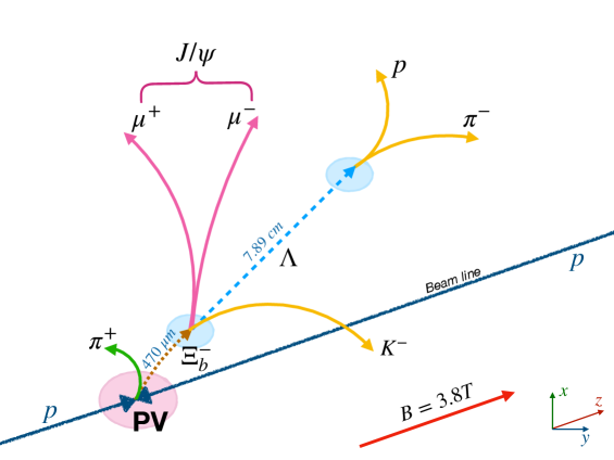
Figure 1: The $\PGXstzb\to\PGXmb\PGpp$ decay topology, where the $\PGXmb$ baryon decays to $\PGy\PGXm$ with $\PGy\to\PGmp\PGmm$ (upper) or $\PJGy\PGL\PKm$ (lower), where refers to the $\PJGy$ and $\PGyP{2S}$ mesons. The distances given are the average decay lengths, $c\tau$.

We also determine the $\PGXstzb$ baryon mass and natural width, using the $\PGXstzb\to\PGXmb\PGpp$ decay. The ground-state $\PGXmb$ is reconstructed via its decays to $\PJGy\PGXm$, $\PGyP{2S}\PGXm$, and $\PJGy\PGL\PKm$. For the $\PGXmb\to\PGyP{2S}\PGXm$ decay, both $\PGyP{2S}\to\PJGy\PGpp\PGpm$, with $\PJGy\to\PGmp\PGmm$, and $\PGyP{2S}\to\PGmp\PGmm$ modes are used in the analysis, and $\PGXm$ is again reconstructed via the $\PGL\PGpm$ channel. For the $\PGXmb\to\PJGy\PGL\PKm$ decay, the presence of the partially reconstructed mode $\PJGy\PGSz\PKm$, where the low-energy photon from the $\PGSz\to\PGL\PGg$ decay is undetected, is included in the fit to the $\PGXmb\PGpp$ invariant mass spectrum. Pictorial representations of the decay topologies for $\PGXstzb\to\PGXmb\PGpp$ are shown in Fig. 1.

We also measure the ratio of the production cross sections $R_{\PGXstzb}$ for $\PGXstzb$ and $\PGXmb$ using the expression:

$$R_{\PGXstzb}=\dfrac{\sigma(\Pp\Pp\to\PGXstzb X)\,\mathcal{B}(\PGXstzb\to\PGXmb\PGpp)}{\sigma(\Pp\Pp\to\PGXmb X)}=\dfrac{N(\PGXstzb\to\PGXmb\PGpp)}{N(\PGXmb)}\dfrac{\epsilon(\PGXmb)}{\epsilon(\PGXstzb\to\PGXmb\PGpp)},$$ (2)

where $N$ and $\epsilon$ refer to similar quantities as those in Eq. (1). Following an analogous CMS measurement of the c2S+ and c∗2S+ production cross section ratios [BPH19001], the $\PGXmb$ baryon is reconstructed in the phase space region defined by the $\PGXmb$ baryon transverse momentum $\pt>15$and rapidity $\abs{y}<2.4$; however, this measured ratio is intended to be representative of the entire phase space, given the small mass difference between the $\PGXstzb$ and $\PGXmb$ particles. The $\PGXstzb$ baryon was the first new particle observed by the CMS Collaboration, using 5of data from 2011 [BPH12001]. With this paper we significantly improve and enrich our previous results for this state. Tabulated results are provided in the HEPData record for this analysis [hepdata].

0.2 The CMS detector and simulated event samples

The central feature of the CMS apparatus is a superconducting solenoid of 6m internal diameter, providing a magnetic field of 3.8T. Within the solenoid volume are a silicon pixel and strip tracker, a lead tungstate crystal electromagnetic calorimeter, and a brass and scintillator hadron calorimeter, each composed of a barrel and two endcap sections. Forward calorimeters extend the pseudorapidity ($\eta$) coverage provided by the barrel and endcap detectors. Muons are measured in gas-ionization detectors embedded in the steel flux-return yoke outside the solenoid. A more detailed description of the CMS detector, together with a definition of the coordinate system used and the relevant kinematic variables, can be found in Ref. [CMS]. More recent changes to the detector are described in Ref. [CMS_Run3]

Muons are measured in the range $\abs{\eta}<2.4$, with detection planes made using three technologies: drift tubes, cathode strip chambers, and resistive plate chambers. The single-muon trigger efficiency exceeds 90% over the full $\eta$ range, whereas the efficiency to reconstruct and identify muons is greater than 96%. Matching muons identified in the muon system to tracks measured in the silicon tracker results in a relative resolution for muons with up to 100of 1% in the barrel and 3% in the endcaps [CMS_muons]. The silicon tracker used in 2016 measured charged particles within the range $\abs{\eta}<2.5$. For nonisolated particles of $1<\pt<10\GeV$ and $\abs{\eta}<1.4$, the track resolutions were typically 1.5% in and 25–90 (45–150)in the transverse (longitudinal) impact parameter [CMS_tracks]. At the start of 2017, a new pixel detector was installed [Phase1Pixel]; the upgraded tracker measured particles up to $\abs{\eta}<3$ with typical resolutions of 1.5% in and 20–75in the transverse impact parameter [DP-2020-049] for nonisolated particles of $1<\pt<10\GeV$. The default track selection used in CMS analyses is the “high-purity” requirement. Because low momentum and displaced tracks share some features with nongenuine tracks such as not pointing back to the $\Pp\Pp$ collision vertex and having fewer measurement points, the high-purity selection is less efficient for these tracks and so the less-restrictive “loose” requirement is often used.

Events of interest are selected using a two-tiered trigger system [Khachatryan:2016bia]. The first level (L1), composed of custom hardware processors, uses information from the calorimeters and muon detectors to select events at a rate of around 100kHz within a fixed latency of about 4 [Sirunyan:2020zal]. The second level, known as the high-level trigger (HLT), consists of a farm of computing processors running a version of the full event reconstruction software optimized for fast processing, and reduces the event rate to around 1kHz before data storage. The events used in this analysis were selected at L1 by requiring the presence of at least two muons, and at the HLT by requiring that the two muons have opposite sign (OS), with various $\abs{\eta}$ and thresholds, compatible with being produced in the dimuon decay of $\PJGy$ or $\PGyP{2S}$ mesons by requiring the corresponding invariant mass windows.

The  8.240 package [Pythia8] with the CP5 underlying event tune [CMS:2019csb] is used to simulate the production of the $\PGXmb$ and $\PGXstzb$ states (where the $\PGSzb$ baryon, with a modified mass value, is used as a proxy for the $\PGXstzb$ state). The $\PGXstzb\to\PGXmb\PGpp$, $\PGXmb\to\PJGy\PGXm$, $\PGXmb\to\PGyP{2S}\PGXm$, $\PGXmb\to\PJGy\PGL\PKm$ (including $\PGXmb\to\PJGy\PGSz\PKm$, $\PGSz\to\PGL\PGg$), $\PGyP{2S}\to\PGmp\PGmm$, $\PGyP{2S}\to\PJGy\PGpp\PGpm$, and $\PJGy\to\PGmp\PGmm$ decays are modeled with  1.6.0 [EvtGen], where final-state photon radiation is included using  3.61 [PHOTOS, PHOTOS_2]. The generated MC events are then passed to a detailed -based simulation [GEANT4] of the CMS detector, which includes the long-lived hyperon decays $\PGXm\to\PGL\PGpm$ and $\PGL\to\Pp\PGpm$. The simulated events are then put through the same trigger and reconstruction algorithms used for the collision data. The simulation includes effects from multiple $\Pp\Pp$ interactions in the same or nearby bunch crossings (pileup) with a multiplicity distribution matching that in data.

0.3 Event reconstruction and selection

The $\PGXmb$ ground state is reconstructed using two main decay modes: $\PGXmb\to\PGy\PGXm$ (followed by $\PGy\to\PGmp\PGmm$), where refers to the $\PJGy$ and $\PGyP{2S}$ mesons, or $\PGXmb\to\PJGy\PGL\PKm$. We also reconstruct the decay chain $\PGXmb\to\PGyP{2S}\PGXm$, $\PGyP{2S}\to\PJGy\PGpp\PGpm$ to increase the number of events for the $\PGXmb\PGpp$ studies. In all the cases, the $\PJGy$ meson is identified through its dimuon decay. The selection criteria, described below, are mainly inherited from Ref. [BPH20004].

The reconstruction chain requires two OS muons forming a good-quality vertex, passing the CMS soft-muon selection [CMS_muons], and with each having $\pt(\PGm)>3\GeV$ and $\abs{\eta(\PGm)}<2.4$. To be of good quality, the fit to a dimuon common vertex must have a $\chi^{2}$ vertex fit probability greater than 1%. These requirements reinforce those applied at the trigger level during the online data taking. A $\PJGy$ or $\PGyP{2S}$ candidate is required to have a dimuon invariant mass within 100of the corresponding world-average mass [PDG], which is about 3 times the mass resolution. Further, a kinematic constraint to the known meson mass [PDG] is applied to the selected dimuon candidates.

The $\PGL$ candidates are formed from displaced two-prong vertices, assuming the decay $\PGL\to\Pp\PGpm$, as described in Ref. [CMS_tracks_V0]. The higher-momentum track is associated with the proton and the lower-momentum track with the pion. A $\PGL$ candidate must have $\pt>1.8\GeV$, and the $\Pp\PGpm$ invariant mass must be within 10of the known $\PGL$ mass [PDG] after the tracks are refit to a common vertex, corresponding to about 3 times the mass resolution. The vertex fit is then repeated with the $\Pp\PGpm$ invariant mass constrained to the $\PGL$ mass, and its momentum recomputed. The $\chi^{2}$ probability of this fit must be greater than 1%.

For the $\PGXmb\to\PGy\PGXm$ channel, the $\PGXm$ candidates are reconstructed by combining each selected $\PGL$ candidate with a charged particle track, assumed to be a pion. The track must have $\pt>0.3\GeV$ and satisfy the loose requirement [CMS_tracks]. A kinematic vertex fit of the $\PGXm\to\PGL\PGpm$ decay is performed, and the $\chi^{2}$ probability is required to be greater than 1%. The $\PGL\PGpm$ invariant mass must be within 10of the known $\PGXm$ mass [PDG], which is about 3 times the mass resolution. The resulting $\PGXm$ candidate must have $\pt>2.5\GeV$. Because $\PGL$ particles mainly decay much further from the $\PGXm$ decay vertex than our vertex resolution, we set a requirement on the pointing angle $\cos\alpha(\PGL,\PGXm)>0.99$ between the momentum of the $\PGL$ candidate and the vector from the $\PGXm$ decay vertex to the $\PGL$ decay vertex in the plane perpendicular to the beam direction (the transverse plane).

To reconstruct the decay chain $\PGXmb\to\PGyP{2S}\PGXm$, $\PGyP{2S}\to\PJGy\PGpp\PGpm$, two additional OS tracks passing the high-purity requirement [CMS_tracks] are assigned the charged pion mass and added to the process. The higher-momentum pion must have $\pt>0.6\GeV$, and the other pion $\pt>0.35\GeV$. The invariant mass of the $\PGyP{2S}$ candidate, calculated via the formula $M(\PGmp\PGmm\PGpp\PGpm)-M(\PGmp\PGmm)+m^{\mathrm{PDG}}(\PJGy)$, is required to be within 18of the known $\PGyP{2S}$ mass [PDG], corresponding to about 3 times the mass resolution. Using this variable removes the $\PJGy\to\PGmp\PGmm$ detector invariant mass resolution from the measurement of the $M(\PGmp\PGmm\PGpp\PGpm)$ invariant mass. Here, and throughout the paper, the symbol $M$ represents a reconstructed invariant mass and $m^{\mathrm{PDG}}$ the PDG world-average mass [PDG].

The $\PGXmb$ candidates are selected by using the $\PGmp$, $\PGmm$, and $\PGXm$ particles in a kinematic fit that constrains their momentum vectors to a common vertex and the dimuon invariant mass to the world-average $\PJGy$ or $\PGyP{2S}$ mass [PDG]. For the decay chain $\PGXmb\to\PGyP{2S}\PGXm$, $\PGyP{2S}\to\PJGy\PGpp\PGpm$, the two additional pions described above are added to the $\PGXmb$ vertex fit. From all the reconstructed $\Pp\Pp$ collision vertices in an event, the primary vertex (PV) is chosen as the one with the smallest pointing angle. The pointing angle is the angle between the $\PGXmb$ candidate momentum and the vector joining the PV with the reconstructed $\PGXmb$ candidate decay vertex. If any of the tracks used in the $\PGXmb$ candidate reconstruction are included in the fit of the chosen PV, they are removed, and the PV is refit. The selected $\PGXmb$ candidates are required to have $\pt(\PGXmb)>10\GeV$ and a $\chi^{2}$ vertex fit probability greater than 1%. The pion from the $\PGXm\to\PGL\PGpm$ decay must satisfy an impact parameter significance requirement $d_{xy}/\sigma_{d_{xy}}>1$, where $d_{xy}$ is the closest distance between the track and the chosen PV in the transverse plane, and $\sigma_{d_{xy}}$ is its uncertainty. For the decay chain $\PGXmb\to\PGyP{2S}\PGXm$, $\PGyP{2S}\to\PJGy\PGpp\PGpm$, we require that the two pion tracks each have $d_{xy}/\sigma_{d_{xy}}>0.4$. The pointing angle $\alpha$ between the $\PGXm$ momentum and the vector from the $\PGXmb$ decay vertex to the $\PGXm$ vertex in the transverse plane must satisfy $\cos{\alpha(\PGXm,\PGXmb)}>0.999$. The analogous angle between the $\PGXmb$ momentum and the vector from the PV to the $\PGXmb$ vertex is required to have $\cos{\alpha(\PGXmb,\text{PV})}>0.99$. Additionally, the distance $L_{xy}$ between the PV and the $\PGXmb$ decay vertex in the transverse plane must fulfill the requirement $L_{xy}/\sigma_{L_{xy}}>3$, where $\sigma_{L_{xy}}$ is its uncertainty.

For the $\PGXmb\to\PJGy\PGL\PKm$ decay channel, the $\PJGy$ and $\PGL$ candidates are reconstructed in the same way as described above, with the additional requirement $\pt(\PGL)>2\GeV$. However, instead of adding a pion track to the subsequent $\PGXm\to\PGL\PGpm$ fit, a charged particle track with a kaon mass assignment is selected. The track must have $\pt>1.4\GeV$ and satisfy the high-purity requirement [CMS_tracks]. The $\PGXmb$ candidates are obtained by performing a kinematic vertex fit to the $\PGmp$, $\PGmm$, $\PGL$, and $\PKm$ candidates, along with the same $\PJGy$ mass constraint and PV selection as for the $\PGXmb\to\PGy\PGXm$ channel. The kaon impact parameter significance must satisfy $d_{xy}/\sigma_{d_{xy}}>0.5$ with respect to the chosen PV. Because of the higher background in this channel more restrictive kinematic and topological requirements are applied: $\pt(\PGXmb)>15\GeV$ and $\cos{\alpha(\PGXmb,\text{PV})}>0.999$, along with the same requirements as above on the vertex fit and $L_{xy}/\sigma_{L_{xy}}$.

Since the lifetime of the excited $\PGXb$ states is expected to be negligible, the $\PGXmb\PGpp$ candidates are formed by combining the selected $\PGXmb$ candidates with each charged particle track originating from the PV and satisfying the loose requirement [CMS_tracks] as done in Ref. [BPH18007], which are given the charged pion mass. The pion charge must be opposite to that of the pion from $\PGXm\to\PGL\PGpm$ or the kaon from $\PGXmb\to\PJGy\PGL\PKm$. The mass difference variable $\Delta M=M(\PGXmb\PGpp)-M(\PGXmb)-m^{\mathrm{PDG}}_{\PGpp}$ is used instead of $M(\PGXmb\PGpp)$ since it is characterized by a better mass resolution as the effect of the $\PGXmb$ mass resolution is removed. From simulation studies, this variable is found to be insensitive to potential mass shifts caused by the missing low-energy photon from the $\PGSz\to\PGL\PGg$ decay. As developed in Ref. [BPH19003], the $\PGXmb$ candidate and all the tracks forming the PV are refit to a common vertex, further improving the $\PGXmb\PGpp$ invariant mass resolution from $1.07\pm 0.07$ to $0.74\pm 0.04\MeV$ (statistical uncertainties only), as determined from simulation studies. If multiple $\PGXstzb$ candidates (where the multiplicity comes from the soft pion reconstruction) in an event pass the selection requirements (which happens in 10–15% of events depending on the $\PGXmb$ channel), only the highest candidate is kept, which is found from simulation studies to improve the signal purity.

0.4 Observation of the $\PGXmb\to\PGyP{2S}\PGXm$ decay and studies of the $\PGXmb$ signal

The invariant mass distributions of the selected $\PJGy\PGXm$, $\PJGy\PGL\PKm$, and $\PGyP{2S}\PGXm$ (with both $\PGyP{2S}\to\PGmp\PGmm$ and $\PGyP{2S}\to\PJGy\PGpp\PGpm$) candidates are shown in Fig. 2. An unbinned extended maximum likelihood fit is performed on each of these distributions. For all four channels, the signal component is described using the sum of two Gaussian functions with a common mean, whose widths and ratio between them are fixed to those determined from MC simulation. However, both widths are allowed to scale by the same free parameter in the fit to give a better description of the data. The background is described with a first-order polynomial for the $\PJGy\PGXm$ and $\PGyP{2S}\PGXm$ channels, and an exponential function for the $\PJGy\PGL\PKm$. In the latter fit, the signal contribution from the partially reconstructed $\PGXmb\to\PJGy\PGSz\PKm$ decays is taken into account by including an asymmetric Gaussian (also known as skew normal) function in the fit, whose shape parameters are fixed to those found from simulation studies.

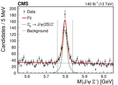
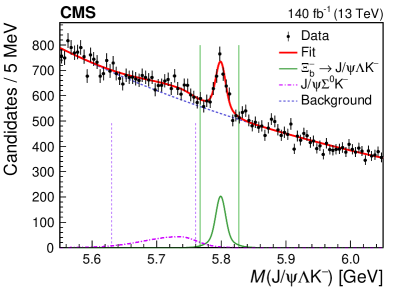
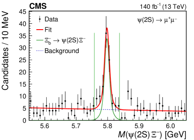
Figure 2: Invariant mass distributions of the selected $\PJGy\PGXm$ (upper left), $\PJGy\PGL\PKm$ (upper right), and $\PGyP{2S}\PGXm$ [lower row, with $\PGyP{2S}\to\PGmp\PGmm$ (left) and $\PGyP{2S}\to\PJGy\PGpp\PGpm$ (right) candidates]. The data are shown by the points, while the vertical bars represent the statistical uncertainties. The overall fit result is shown by the solid red curve, with the signal and background contributions given by the solid green and dashed blue curves, respectively. The vertical lines around each peak display the mass window required for a $\PGXmb$ candidate to be used in the $\PGXstzb$ studies. The dotted-dashed curve in the upper right plot shows the fitted contribution from the $\PGXmb\to\PJGy\PGSz\PKm$ decay, with the accompanying vertical dotted lines indicating the mass window for this mode.

The number of signal events $N$, the mean $\PGXmb$ mass $m_{\PGXmb}^{\text{fit}}$, and the effective $\PGXmb$ width $\sigma_{\text{eff}}$ from the fits to the $\PGXmb$ invariant mass distributions for each of the $\PGXmb$ decay channels. The uncertainties are statistical only. lccc Decay channel & $N$ $m_{\PGXmb}^{\text{fit}}$ () $\sigma_{\text{eff}}$ ()
$\PGXmb\to\PJGy\PGXm$ $846\pm 40\phantom{1}$ $5797.1\pm 0.6$ $16.3\pm 1.0$
$\PGXmb\to\PJGy\PGL\PKm$ $920\pm 98\phantom{1}$ $5798.8\pm 0.9$ $11.9\pm 1.5$
$\PGXmb\to\PJGy\PGSz\PKm$ $880\pm 170$
$\PGXmb\to\PGyP{2S}\PGXm$ (with $\PGyP{2S}\to\PGmp\PGmm$) $\phantom{8}74\pm 11\phantom{0}$ $5797.7\pm 1.4$ $11.1\pm 2.0$
$\PGXmb\to\PGyP{2S}\PGXm$ (with $\PGyP{2S}\to\PJGy\PGpp\PGpm$) $\phantom{8}90\pm 14\phantom{0}$ $5797.2\pm 1.7$ $13.1\pm 2.8$

The number of signal events $N$, the mean $\PGXmb$ mass $m_{\PGXmb}^{\text{fit}}$, and the effective $\PGXmb$ width $\sigma_{\text{eff}}$ from the fit are given in Table 0.4 for each of the $\PGXmb$ decay channels, along with their statistical uncertainties. The value of $\sigma_{\text{eff}}$ is calculated as $\sqrt{\smash[b]{f_{1}\sigma_{1}^{2}+(1-f_{1})\sigma_{2}^{2}}}$, where $\sigma_{1}$ ($\sigma_{2}$) is the width of the first (second) Gaussian, and $f_{1}$ is the fraction of signal events from the fit associated with the first Gaussian function. The measured resolution of the different channels is within the expectations from the available phase space and the final state threshold proximity. The fitted $\PGXmb$ mass values are consistent with the world-average value $m_{\PGXmb}^{\mathrm{PDG}}=5797.0\pm 0.6\MeV$ [PDG].

This is the first observation of the $\PGXmb\to\PGyP{2S}\PGXm$ decay. Its local statistical significance is evaluated with the likelihood ratio technique, comparing the likelihood value from a fit to a signal-plus-background hypothesis to that for a background-only hypothesis. Since the conditions of Wilks’ theorem [Wilks_LL_ratio] are satisfied, the asymptotic formulae of Ref. [Cowan_ssymptotic] (Eqs. (12) and (52)) are used to determine the $\PGXmb\to\PGyP{2S}\PGXm$ signal significance, which is found to be well above 5 standard deviations for both the $\PGyP{2S}\to\PGmp\PGmm$ and $\PGyP{2S}\to\PJGy\PGpp\PGpm$ modes.

For the $\PGXmb\PGpp$ studies described in the next section, the $\PGXmb$ candidates must have an invariant mass within 40 (30)of the $m_{\PGXmb}^{\text{fit}}$ value for the $\PJGy\PGXm$ and $\PGyP{2S}\PGXm$ ($\PJGy\PGL\PKm$) decay channels. This corresponds to about (2.5–3) times $\sigma_{\text{eff}}$, as shown by the solid vertical lines around the peaks in Fig. 2. For the partially reconstructed $\PJGy\PGSz\PKm$ decay channel, a mass window of 5.63–5.76, as in Ref. [BPH20004] and shown by the vertical dotted lines in Fig. 2 (upper right), is used for the reconstructed $\PGXmb$ mass.

0.5 Studies of the $\PGXstzb$ baryon

The measured $\Delta M$ distributions found by combining the selected $\PGXmb$ candidates, as defined in Section 0.4, with charged particle tracks, consistent with coming from the PV and assumed to be pions, are shown in Fig. 3. The distributions are shown separately for the $\PGXmb\to\PJGy\PGXm$, $\PGXmb\to\PGyP{2S}\PGXm$ (combined $\PGyP{2S}\to\PJGy\PGpp\PGpm$ and $\PGyP{2S}\to\PGmp\PGmm$ modes), $\PGXmb\to\PJGy\PGL\PKm$, and $\PGXmb\to\PJGy\PGSz\PKm$ channels. A significant near-threshold peak is evident in all 4 distributions, in agreement with previous CMS [BPH12001] and LHCb [LHCb_XibStar0, LHCb_Xbss] results. The $\Delta M$ distribution for the same-sign $\PGXmb\PGpm$ control sample is also displayed in Fig. 3. It shows no evidence of a peak and is consistent with the $\PGXmb\PGpp$ combinatorial background. No other structures are observed in this $\Delta M$ region for either the $\PGXmb\PGpp$ or $\PGXmb\PGpm$ distributions.

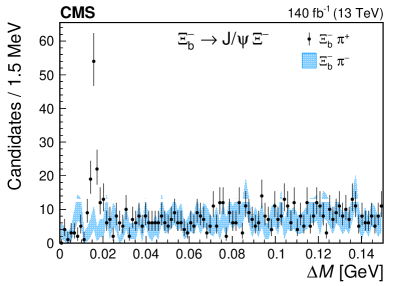
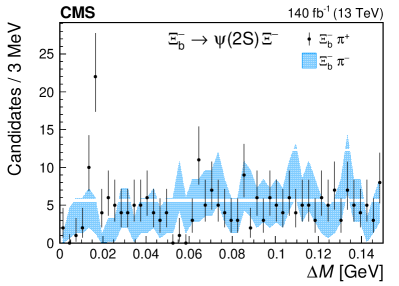
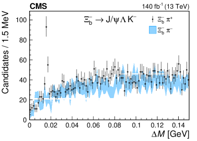
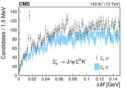
Figure 3: The mass difference $\Delta M$ distribution of the selected $\PGXmb\PGppm$ candidates for the decay channel labeled on each plot. The points show the correct-sign combinations and the blue bands the wrong-sign. The vertical bars on the points and the length of the bands represent the statistical uncertainties in each distribution, respectively.

We fit the $\PGXstzb$ signal using a relativistic Breit–Wigner function, which accounts for the non-negligible natural width $\Gamma(\PGXstzb)$, convolved with a Gaussian function describing the invariant mass resolution, whose parameters are extracted from MC simulation. Lattice QCD calculations [Th:lattice] give $\Gamma(\PGXstzb)=0.51\pm 0.16\MeV$, the ${}^{3}P_{0}$ model predicts 0.85 [Th:3P0_model], and the latest LHCb result finds $\Gamma(\PGXstzb)=0.87\pm 0.06\pm 0.05\MeV$ [LHCb_Xbss]. The simulation studies predict that the invariant mass resolution is slightly different for each $\PGXmb$ baryon decay channel, except for the $\PGXmb\to\PJGy\PGSz\PKm$ mode, where the missing low-energy photon from the $\PGSz$ baryon decay produces a much wider peak with a 26% larger mass resolution. In all cases, the measured widths from the fully reconstructed decay modes are in agreement within their uncertainties.

An unbinned extended maximum likelihood simultaneous fit of all four channels is applied, where the $\PGXstzb$ mass and natural width are constrained to be equal for all the channels, while the mass resolutions, yields, and background parameters are different. The background component is modeled with a threshold function $(\Delta M)^{\alpha}$, where $\alpha$ is a free parameter. The fit results are shown in Fig. 4, and the fitted signal yields are given in Table 0.5.

The measured mass difference and natural width of the $\PGXstzb$ state are $\Delta M^{\text{fit}}=15.810\pm 0.077\MeV$ and $\Gamma(\PGXstzb)=0.87\,^{+0.22}_{-0.20}\MeV$, respectively, where the uncertainties are statistical only.

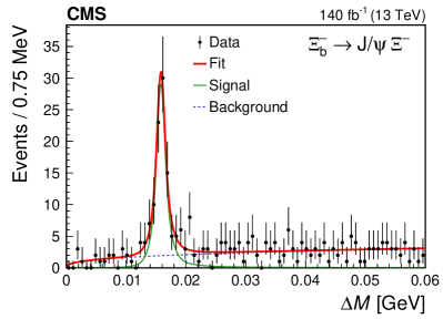
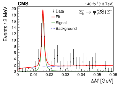
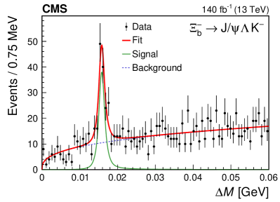
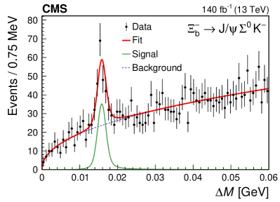
Figure 4: Results of the simultaneous fits to the $\Delta M$ invariant mass distributions for the $\PGXstzb$ candidates in the decay channels given in each plot. The points show the data, with the vertical bars representing the statistical uncertainty. The solid red curve displays the overall fit result, with the solid green and dashed blue curves showing the signal and background contributions, respectively.

The fitted signal yields of the $\PGXstzb\to\PGXmb\PGpp$ decay for each of the listed $\PGXmb$ decay channels. Uncertainties are statistical only. lc Decay channel $N(\PGXstzb)$
$\PGXmb\to\PJGy\PGXm$ $\phantom{1}97\,^{+13}_{-12}$
$\PGXmb\to\PGyP{2S}\PGXm$ $\phantom{1}24\,^{+6\phantom{2}}_{-5}$
$\PGXmb\to\PJGy\PGL\PKm$ $124\,^{+17}_{-16}$
$\PGXmb\to\PJGy\PGSz\PKm$ $155\,^{+22}_{-20}$

0.6 Efficiency and production ratio measurements

While in general the analysis uses events collected by a combination of different dimuon HLT paths, for the measurements of the ratios of efficiencies and the resulting branching fractions and production cross sections, a single dedicated trigger suitable for the decay topology is required in order to simplify the efficiency estimations and reduce the trigger-related systematic uncertainty. For the $\PGXmb\to\PJGy\PGXm$ and $\PGXmb\to\PGyP{2S}\PGXm$ channels, we use an inclusive dimuon HLT path, requiring the presence in the event of a $\PJGy$ ($\PGyP{2S}$) meson with exceeding 25 (18) and decaying into two OS muons. This HLT path is only used for the 2017–2018 sample, while for the 2016 sample the similar trigger requires a minimum of 20 (13) for the $\PJGy$ ($\PGyP{2S}$) meson. In the case of the $\PGXmb\to\PJGy\PGL\PKm$ channel, we use an HLT path requiring the presence of a $\PJGy\to\PGmp\PGmm$ decay and an additional track consistent with originating from the dimuon vertex and having $d_{xy}/\sigma_{d_{xy}}>2$. The dimuon vertex must also be displaced from the PV, by requiring $L_{xy}/\sigma_{L_{xy}}>3$.

These requirements are much stricter than those discussed in Section 0.3 — most from $\PGXmb$ decays are populated within the 10–20range of . Thus, using them causes a significant decrease in the signal yields for the $\PGy\PGXm$ channels. Redoing the fitting procedure with the new requirements leads to total signal yields of $103^{+14}_{-13}$ and $38^{+8}_{-7}$ for $\PGXmb\to\PJGy\PGXm$ and $\PGXmb\to\PGyP{2S}\PGXm$ ($\PGyP{2S}\to\PGmp\PGmm$ mode), respectively. The $\PGXmb\to\PJGy\PGL\PKm$ signal with the tighter HLT requirement results in $606^{+67}_{-64}$ events. The fits to the $\PGXstzb\to\PGXmb\PGpp$ $\Delta M$ distributions are performed separately for each of the decay channels, with $\Gamma(\PGXstzb)$ fixed to the value found from the simultaneous fit. The resulting signal yields are $13\pm 4$ and $74\pm 11$ for the $\PJGy\PGXm$ and $\PJGy\PGL\PKm$ decay modes, respectively.

The efficiencies for the signal and normalization channels are calculated using simulated MC samples of events that have passed the more-restrictive HLT paths described above. The total efficiency includes several factorizable contributions such as the trigger, detector acceptance, and decay channel reconstruction efficiencies. The detector acceptance term is calculated as the ratio of the number of generator-level events within the CMS kinematic acceptance to the number of generated events without any restrictions (within the full phase space region). Efficiencies for different years of data taking are estimated separately and then combined with weights corresponding to the integrated luminosity collected in each year.

Since we measure branching fractions and production cross sections with respect to normalization channels, only the ratios of such efficiencies are needed. Thus, for example, the systematic uncertainties associated with the muon, charged particle track, and $\PGL$ candidate reconstruction are reduced. Table 0.6 reports three efficiency ratios, where the first is used in measuring the quantity $R$, the ratio of branching fractions defined in Eq. (1), and the latter two for finding the $\PGXstzb$/ $\PGXmb$ production cross section ratio using two different decay channels: $\PJGy\PGXm$ and $\PJGy\PGL\PKm$.

The measured efficiency ratios and their statistical uncertainties. cc Efficiency ratio Value
 $\epsilon(\PGXmb\to\PJGy\PGXm)/\epsilon(\PGXmb\to\PGyP{2S}\PGXm,\,\PGyP{2S}\to\PGmp\PGmm)$ $0.304\pm 0.014$
$\epsilon(\PGXmb\to\PJGy\PGXm)/\epsilon(\PGXstzb\to\PGXmb\PGpp,\,\PGXmb\to\PJGy\PGXm)$ $1.645\pm 0.108$
$\epsilon(\PGXmb\to\PJGy\PGL\PKm)/\epsilon(\PGXstzb\to\PGXmb\PGpp,\,\PGXmb\to\PJGy\PGL\PKm)$ $1.941\pm 0.085$

Using the measured signal yields, the efficiency ratio, and Eq. (1), we determine the ratio $R$ of the branching fraction for the newly observed $\PGXmb\to\PGyP{2S}\PGXm$ decay to that of the $\PGXmb\to\PJGy\PGXm$ decay to be

$$R=0.84^{+0.21}_{-0.19},$$

where the uncertainty is coming from the uncertainty in the measured yields. The uncertainty in the ratio of efficiencies is treated separately as a systematic uncertainty, as described in Section 0.7.1.

Applying Eq. (2), the ratio $R_{\PGXstzb}$ of the $\PGXstzb$ to $\PGXmb$ production is separately measured using two $\PGXmb$ decay channels: $\PJGy\PGXm$ and $\PJGy\PGL\PKm$. The results are

$$R_{\PGXstzb}^{\PJGy\PGXm}=0.21\pm 0.07$$

and

$$R_{\PGXstzb}^{\PJGy\PGL\PKm}=0.24\pm 0.04,$$

where the uncertainties are statistical only (again, the efficiency uncertainties are discussed in Section 0.7.1). Both values, obtained with fully independent data and simulation samples, are in good agreement with each other and with the previous measurement by the LHCb Collaboration [LHCb_XibStar0].

0.7 Systematic uncertainties

The systematic uncertainties in the measurements given above are divided into two categories. The first is related to the uncertainties in the measured efficiency ratios and the $\PGXmb$ and $\PGXstzb$ signal yields. The second covers the uncertainties in the measured mass difference and natural width of the $\PGXstzb$ baryon.

0.7.1 Systematic uncertainties in the measured ratios

Many systematic uncertainties related to muon reconstruction and identification, trigger effects and efficiencies, and charged particle track and $\PGL$ candidate reconstruction cancel out in the measured ratio $R$ due to the identical topologies of the $\PGXmb\to\PGyP{2S}\PGXm$ and $\PGXmb\to\PJGy\PGXm$ decays. There is a similar cancellation in the determination of the production cross section ratio $R_{\PGXstzb}$, where the only topological difference between $\PGXstzb$ and $\PGXmb$ is an additional track from the $\PGXstzb\to\PGXmb\PGpp$ decay.

The systematic uncertainty related to the choice of fit functions used to describe the signal and background shapes in the invariant mass fits is evaluated by varying the functions used and recording the change in the number of signal events. For the three $\PGXmb$ decay channels, we first perform the fit with the resolution scaling parameter for the sum of two Gaussian functions set to unity and note the change in the fit results. We then use a Student’s t distribution [Studentt] to model the signal, with the mean and the width allowed to be free and the $n$ parameter (corresponding to the number of degrees of freedom) fixed from the simulation. This function, being symmetric and bell-shaped, also models a heavy-tailed distribution and thus is found to be a reliable alternative to the sum of two Gaussian functions. A single Gaussian function with free parameters is also tried for fitting the $\PGyP{2S}\PGXm$ and $\PJGy\PGXm$ signals. Using the largest change in the number of events, the resulting systematic uncertainty in $R$ from this source is 8.8%.

Two alternative background functions are considered in fitting the $\PJGy\PGXm$ and $\PGyP{2S}\PGXm$ invariant mass distributions: an exponential function and a second-order polynomial. For the more complicated background shape in the $\PJGy\PGL\PKm$ distribution, we switch from an exponential function to a second-order polynomial. The resulting systematic uncertainty in $R$ from this source is estimated as 4.5%. The combined signal-plus-background $\PGXmb$ fit model uncertainties are estimated as 4.0 and 6.9% in the $R_{\PGXstzb}^{\PJGy\PGXm}$ and $R_{\PGXstzb}^{\PJGy\PGL\PKm}$ values, respectively.

The alternative functions used in fitting the $\PGXstzb\to\PGXmb\PGpp$ $\Delta M$ distribution are described in the next subsection when the systematic uncertainties in the measured $\PGXstzb$ mass and width are discussed. The resulting systematic uncertainties due to the fitting functions in the $R_{\PGXstzb}$ production cross section ratio are 7.7 and 6.7% for the $\PJGy\PGXm$ and $\PJGy\PGL\PKm$ decay modes, respectively.

For the $R$ measurement, given that we are using different HLT paths for the $\PGXmb\to\PJGy\PGXm$ and the $\PGXmb\to\PGyP{2S}\PGXm$ signals, a cross-check of the correctness and robustness of such a procedure is performed. The similar branching fraction ratio $R_{\PBp}=\mathcal{B}(\PBp\to\PGyP{2S}\PKp)/\mathcal{B}(\PBp\to\PJGy\PKp)$ was measured with the triggers we use for the $\PGXmb$ signals, and the resulting value of $0.601\pm 0.030$ is consistent with the world-average value [PDG] $0.605\pm 0.021$. The 5% precision of the $R_{\PBp}$ value is taken conservatively as an additional systematic uncertainty in the $R$ measurement.

As mentioned above, an additional source of uncertainty in the $R_{\PGXstzb}$ measurement comes from identifying the extra pion in the $\PGXstzb\to\PGXmb\PGpp$ decay. The uncertainty in the tracking reconstruction efficiency for the low-pion is estimated as 5.2% [BPH18003].

The uncertainty related to the finite size of the MC samples is also considered as a systematic uncertainty. It is estimated from the statistical uncertainty in the determinations of the efficiency ratios from the MC simulation. This corresponds to a systematic uncertainty of 4.6% in $R$, and 6.5 and 4.4% in $R_{\PGXstzb}$ for the $\PJGy\PGXm$ and $\PJGy\PGL\PKm$ modes, respectively.

The systematic uncertainties in the $R$ and $R_{\PGXstzb}$ measurements are summarized in Tables 0.7.1 and 0.7.1, respectively, along with the total systematic uncertainties, calculated from the sum in quadrature of the individual sources.

Systematic uncertainties in percent in the ratio $R$ from the different sources and the total uncertainty. lc Source Uncertainty (%)
Signal model 8.8
Background model 4.5
$R_{\PBp}$ uncertainty 5.0
MC finite size 4.6
Total 12.0

Systematic uncertainties in percent in the ratio $R_{\PGXstzb}$ from the different sources and the total uncertainty, separately for the $\PJGy\PGXm$ and $\PJGy\PGL\PKm$ decay modes. lcc Source $\PJGy\PGXm$ (%) $\PJGy\PGL\PKm$ (%)
$\PGXmb$ fit model 4.0 6.9
$\PGXstzb$ fit model 7.7 6.7
Tracking efficiency 5.2 5.2
MC finite size 6.5 4.4
Total 12.0 11.8

0.7.2 Systematic uncertainties in the $\PGXstzb$ baryon mass and width measurements

Several sources of systematic uncertainty are considered in the simultaneous measurement of the $\PGXstzb$ baryon mass difference and natural width. To evaluate the systematic uncertainties related to the choice of functions used to fit the $\PGXstzb$ $\Delta M$ distributions, alternative functions are chosen and the maximum changes in the results of the fit are used to estimate the corresponding systematic uncertainty. We use a Student’s t-distribution [Studentt] as the alternative function to describe the invariant mass resolution, with the shape parameters determined from MC simulation. Fitting the data distributions leads to estimates for the systematic uncertainty of $\pm 0.003\MeV$ in the mass difference, while the change in the natural width is negligible.

We also vary the function used to describe the background in the fit. We use the threshold function described earlier, multiplied by a first-order polynomial, except for the $\PGXmb\to\PGyP{2S}\PGXm$ decay channel, where the number of events is too small to allow a reasonable fit to the background for functions with more parameters. Another alternative model uses the baseline background model to fit the same-sign $\PGXmb\PGpm$ distributions. The $\alpha$ values obtained in these fits are then used as fixed parameters of the simultaneous fit. From this, we estimate systematic uncertainties from this source of $\pm 0.002$ and $\pm 0.04\MeV$ in the mass difference and natural width, respectively.

The systematic uncertainty coming from the choice of the fit range is estimated by varying the $\Delta M$ fit region from $[0,\,0.05]$ to $[0,\,0.09]\GeV$. The maximum deviation of the fit parameters is used as the systematic uncertainty, giving $\pm 0.023$ and $\pm 0.13\MeV$ in the mass difference and natural width, respectively.

The signal shape for the $\PGXstzb$ $\Delta M$ distribution is fit with a Gaussian resolution function, convolved with a relativistic Breit–Wigner (RBW) and a Blatt–Weisskopf barrier factor [Blatt], with the radial parameter in these functions set to $r=3.5\GeV^{-1}$ and the angular momentum (spin) to $\ell=1$. To determine the systematic uncertainty associated with these choices, the fit is repeated with the value of $r$ varied in the range 1–5 $\GeV^{-1}$ and $\ell$ set to 0 or 2. The change in $r$ has a negligible effect, while the spin change leads to systematic uncertainties of $\pm 0.022$ and $\pm 0.02\MeV$ in the mass difference and natural width measurements, respectively.

For the $\PGXmb\to\PJGy\PGXm$ channel, we verify that the mass resolutions obtained in data and simulation agree to within the combined uncertainty of 7.5%. We obtain a systematic uncertainty associated with any potential disagreement in the $\Delta M$ mass resolution between data and simulation by repeating the $\PGXstzb$ fit with the resolutions from MC scaled up or down by 1.075. The resulting systematic uncertainties are $\pm 0.004$ and $\pm 0.08\MeV$ for the mass difference and natural width, respectively.

The systematic uncertainties described above are summarized in Table 0.7.2, together with the total systematic uncertainties, found from the quadrature sum of those from the individual sources.

The systematic uncertainties in in the measurement of the $\PGXstzb$ mass difference and natural width from each of the sources, along with the total uncertainties. lcc Source $\Delta M$ () $\Gamma(\PGXstzb)$ ()
Signal model 0.003 $<0.01$
Background model 0.002 0.04
Fit range 0.023 0.13
RBW shape 0.022 0.02
Mass resolution 0.004 0.08
Total 0.032 0.16