Batched Nonparametric Contextual Bandits

Abstract

We study nonparametric contextual bandits under batch constraints, where the expected reward for each action is modeled as a smooth function of covariates, and the policy updates are made at the end of each batch of observations. We establish a minimax regret lower bound for this setting and propose Batched Successive Elimination with Dynamic Binning (BaSEDB) that achieves optimal regret (up to logarithmic factors). In essence, BaSEDB dynamically splits the covariate space into smaller bins, carefully aligning their widths with the batch size. We also show the suboptimality of static binning under batch constraints, highlighting the necessity of dynamic binning. Additionally, our results suggest that a nearly constant number of policy updates can attain optimal regret in the fully online setting.

1 Introduction

Recent years have witnessed substantial progress in the field of sequential decision making under uncertainty. Especially noteworthy are the advancements in personalized decision making, where the decision maker uses side-information to make customized decision for a user. The contextual bandit framework has been widely adopted to model such problems because of its capability and elegance [35, 53, 6]. In this framework, one interacts with an environment for a number of rounds: at each round, one is given a context, picks an action, and receives a reward. One can update the action-assignment policy based on previous observations and the goal is to maximize the expected cumulative rewards. For example, in online news recommendation, a recommendation algorithm selects an article for each newly arrived user based on the user’s contextual information, and observes whether the user clicks the article or not. The goal is to try to maximize the number of clicks received. Apart from news recommendation, contextual bandits have found numerous applications in other fields such as clinical trials, personalized medicine, and online advertising [30, 62, 13].

At the core of designing a contextual bandit algorithm is deciding how to update the policy based on prior observations. A standard metric of performance for bandit algorithms is regret, which is the expected difference between the cumulative rewards obtained by an oracle who knows the optimal action for every context and that obtained by the actual algorithm under consideration. Many existing regret optimal bandit algorithms require a policy update per observation (unit) [4, 1, 39, 34]. At a first glance, such frequent policy updates are needed so that the algorithm can quickly learn the optimal action under each context and reduce regret. However, this kind of algorithm ignores an important concern in the practice of sequential decision making—the batch constraint.

In many real world scenarios, the data often arrive in batches: the statistician can only observe the outcomes of the policy at the end of a batch, and then decides what to do for the next batch. For example, this batch constraint is ubiquitous in clinical trials: statisticians need to divide the participants into batches, determine a treatment allocation policy before the batch starts, and then observe all the outcomes at the end of the batch [49]. Policy updates are made per batch instead of per unit. In fact, it is infeasible to apply unit-wise policy update in this case because observing the effect of a treatment takes time and if one waits for the result before deciding how to treat the next patient, the entire experiment will take too long to complete when the number of participants is huge. The batch constraint also appears in areas such as online marketing, crowdsourcing, and simulations [8, 50, 31, 15]. Clearly, the batch constraint presents additional challenges to online learning. Indeed, from an information perspective, the statistician’s information set is largely restricted since she can only observe all the responses at the end of a batch. The following questions naturally arise:

Given a batch budget $M$ and a total number of $T$ rounds, how should the statistician determine the size of each batch, and how should she update the policy after each batch? Can the statistician design batch learning algorithms that achieve regret performances on par with the fully online setting using as few policy updates as possible?

1.1 Main contributions

In this work, we address the aforementioned questions under a classical framework for personalized decision making—nonparametric contextual bandits [48, 39]. In this framework, the expected reward associated with each treatment (or arm in the language of bandits) is modeled as a nonparametric smooth function of the covariates [59]. In the fully online setup, seminal works [48, 39] establish the minimax optimal regret bounds for the nonparametric contextual bandits. Nevertheless, under the more challenging setting with the batch constraint, the fundamental limits for nonparametric bandits remain unknown. Our paper aims to bridge this gap. More concretely, we make the following three novel contributions:

• First, we establish a minimax regret lower bound for the nonparametric bandits with the batch constraint $M$. Our proof relies on a simple but useful insight that the worst-case regret over the entire horizon is greater than the worst-case regret over the first $i$ batches for all $1\leq i\leq M$. To fully exploit this insight, for each different batch number $i$, we construct different families of hard instances to target this batch, leading to a maximal regret over this batch.

• In addition, we demonstrate that the aforementioned lower bound is tight by providing a matching upper bound (up to log factors). Specifically, we design a novel algorithm—Batched Successive Elimination with Dynamic Binning (BaSEDB)—for the nonparametric bandits with batch constraints. BaSEDB progressively splits the covariate space into smaller bins whose widths are carefully selected to align well with the corresponding batch size. The delicate interplay between the batch size and the bin width is crucial for obtaining the optimal regret in the batch setting.

• On the other hand, we show the suboptimality of static binning under the batch constraint by proving an algorithm-specific lower bound. Unlike the fully online setting where policies that use a fixed number of bins can attain the optimal regret [39], our lower bound indicates that batched successive elimination with static binning is strictly suboptimal. This highlights the necessity of dynamic binning in some sense under the batch setting, which is uncommon in classical nonparametric estimation.

It is also worth mentioning that an immediate consequence of our results is that $M\gtrsim\log\log T$ number of batches suffices to achieve the optimal regret in the fully online setting. In other words, we can use a nearly constant number of policy updates in practice to achieve the optimal regret obtained by policies that require one update per round.

1.2 Related work

Nonparametric contextual bandits.

[58] introduced the mathematical framework of contextual bandit. The theory of contextual bandits in the fully online setting has been continuously developed in the past few decades. On one hand, [4, 1, 23, 6, 7, 41] obtained learning guarantees for linear contextual bandits in both low and high dimensional settings. On the other hand, [59] introduced the nonparametric approach to model the mean reward function. [48] proved a minimax lower bound on the regret of nonparametric bandit and developed an upper-confidence-bound (UCB) based policy to achieve a near-optimal rate. [39] improved this result and proposed the Adaptively Binned Successive Elimination (ABSE) policy that can also adapt to the unknown margin parameter. Further insights in this nonparametric setting were developed in subsequent works [42, 43, 45, 24, 27, 52, 25, 10, 51, 9]. The smoothness assumption is also adopted in another line of work [37, 36, 33, 11] on the continuum-armed bandit problems. However in contrast to what we study, the reward is assumed to be a Lipschitz function of the action, and the covariates are not taken into considerations.

Batch learning.

The batch constraint has received increasing attention in recent years. [40, 21] considered the multi-armed bandit problem under the batch setting and showed that $O(\log\log T)$ batches are adequate in achieving the rate-optimal regret, compared to the fully online setting. [26, 47] extended batch learning to the (generalized) linear contextual bandits and [46, 56, 17] further studied the setting with high-dimensional covariates. [29, 28] established batch learning guarantees for the Thompson sampling algorithm. [18] considered Lipschitz continuum-armed bandit problem with the batch constraint. Inference for batched bandits was considered in [60]. A concept related to batch learning in literature is called delayed feedback [14, 13, 55, 19]. These works consider the setting where rewards are observed with delay and analyze effects of delay on the regret. [32, 2] studied delayed feedback in nonparametric bandits and the key difference to batch learning is that the batch size is given, whereas in our case, it is a design choice by the statistician. Batch learning’s focus is different to that of delayed feedback in the sense that the former gives the decision maker discretion to choose the batch size which makes it possible to approximate the optimal standard online regret with a small number of batches. Finally, the notion switching cost is intimately related to the batch constraint. [12] studied online learning with low switching cost and obtained minimax optimal regret with $O(\log\log T)$ batches. [5, 61, 20, 57, 44] developed regret guarantees with low switching cost for reinforcement learning. Low switching cost can be interpreted as infrequent policy updates, but it does not require the learner to divide the samples into batches with feedback only becoming available at the end of a batch.

2 Problem setup

We begin by introducing the problem setup for nonparametric bandits with the batch constraint.

A two-arm nonparametric bandit with horizon $T\geq 1$ is specified by a sequence of independent and identically distributed random vectors

$$(X_{t},Y_{t}^{(1)},Y_{t}^{(-1)}),\qquad\text{for }t=1,2,\ldots,T,$$ (1)

where $X_{t}$ is sampled from a distribution $P_{X}$. Throughout the paper, we assume that $X_{t}\in\mathcal{X}\coloneqq[0,1]^{d}$, and $P_{X}$ has a density (w.r.t. the Lebesgue measure) that is bounded below and above by some constants $\underline{c},\bar{c}>0$, respectively. For $k\in\{1,-1\}$ and $t\geq 1$, we assume that $Y_{t}^{(k)}\in[0,1]$ and that

$$\mathbb{E}[Y_{t}^{(k)}\mid X_{t}]=f^{(k)}(X_{t}).$$

Here $f^{(k)}$ is the unknown mean reward function for the arm $k$.

Without the batch constraint, the game of nonparametric bandits plays sequentially. At each step $t$, the statistician observes the context $X_{t}$, and pulls an action $A_{t}\in\{1,-1\}$ according to a rule $\pi_{t}:\mathcal{X}\mapsto\{1,-1\}$. Then she receives the corresponding reward $Y_{t}^{(A_{t})}$. In this case, the rule $\pi_{t}$ for selecting the action at time $t$ is allowed to depend on all the observations strictly anterior to $t$.

In an $M$-batch game, the statistician is asked to divide the horizon $[1:T]$ into $M$ disjoint batches $[1:t_{1}]$, $[t_{1}+1:t_{2}]$, $\ldots,[t_{M-1}+1,T]$. In contrast to the case without the batch constraint, only the rewards associated with timesteps prior to the current batch are observed and available for making decisions for the current batch. More formally, an $M$-batch policy is composed of a pair $(\Gamma,\pi)$, where $\Gamma=\{t_{0,}t_{1,...,}t_{M}\}$ is a partition of the entire time horizon $T$ that satisfies $0=t_{0}<t_{1}<...<t_{M-1}<t_{M}=T$, and $\pi=\{\pi_{t}\}_{t=1}^{T}$ is a sequence of random functions $\pi_{t}:\mathcal{X}\mapsto\{1,-1\}$. Let $\Gamma(t)$ be the batch index for the time $t$, i.e., $\Gamma(t)$ is the unique integer such that $t_{\Gamma(t)-1}<t\leq t_{\Gamma(t)}$. Then at time $t$, the available information for $\pi_{t}$ is only $\{X_{l}\}_{l=1}^{t}\cup\{Y_{l}^{(A_{l})}\}_{l=1}^{\Gamma(t)-1}$, which we denote by $\mathcal{F}^{t}$. The statistician’s policy $\pi_{t}$ at time $t$ is allowed to depend on $\mathcal{F}_{t}$.

The goal of the statistician is to design an $M$-batch policy $(\Gamma,\pi)$ that can compete with an oracle that has perfect knowledge (i.e., the law of $(X_{t},Y_{t}^{(1)},Y_{t}^{(-1)})$) of the environment. Formally, we define the cumulative regret as

$$R_{T}(\pi)\coloneqq\mathbb{E}\left[\sum_{t=1}^{T}\left(f^{\star}(X_{t})-f^{(\pi_{t}(X_{t}))}(X_{t})\right)\right],$$ (2)

where $f^{\star}(x)\coloneqq\max_{k\in\{1,-1\}}f^{(k)}(x)$ is the maximum mean reward one could obtain on the context $x$. Note here we omit the dependence on $\Gamma$ for simplicity.

2.1 Assumptions

We adopt two standard assumptions in the nonparametric bandits literature [48, 39]. The first assumption is on the smoothness of the mean reward functions.

Assumption 1 (Smoothness).

We assume that the reward function for each arm is $(\beta,L)$-smooth, that is, there exist $\beta\in(0,1]$ and $L>0$ such that for $k\in\{1,-1\}$,

$$|f^{(k)}(x)-f^{(k)}(x^{\prime})|\leq L\|x-x^{\prime}\|_{2}^{\beta}$$

holds for all $x,x^{\prime}\in\mathcal{X}$.

The second assumption is about the separation between the two reward functions.

Assumption 2 (Margin).

We assume that the reward functions satisfy the margin condition with parameter $\alpha>0$, that is there exist $\delta_{0}\in(0,1)$ and $D_{0}>0$ such that

$$\mathbb{P}_{X}\left(0<\left|f^{(1)}(X)-f^{(-1)}(X)\right|\leq\delta\right)\leq D_{0}\delta^{\alpha}$$

holds for all $\delta\in[0,\delta_{0}]$.

Assumption 2 is related to the margin condition in classification [38, 54, 3] and is introduced to bandits in [22, 48, 39]. The margin parameter affects the complexity of the problem. Intuitively, a small $\alpha$, say $\alpha\approx 0$, means the two mean functions are entangled with each other in many regions and hence it is challenging to distinguish them; a large $\alpha$, on the other hand, means the two reward functions are mostly well-separated.

From now on, we use $\mathcal{F}(\alpha,\beta)$ to denote the class of nonparametric bandit instances (i.e., distributions over (1)) that satisfy Assumptions 1-2.

Remark 1.

Throughout the paper, we assume that $\alpha\beta\leq 1$. By proposition 2.1 from [48], when $\alpha\beta>1$, one of the arms will dominate the other one for the entire covariate space. The instance is reduced to a multi-armed bandit without covariates which is not the interest of the current paper. Therefore, we focus on the case $\alpha\beta\leq 1$ hereafter.

3 Fundamental limits of batched nonparametric bandits

Somewhat unconventionally, we start with stating a minimax lower bound, as well as its proof, for regret minimization in batched nonparametric contextual bandits. As we will soon see, the proof of the lower bound is extremely instrumental in our development of an optimal $M$-batch policy $(\Gamma,\pi)$, to be detailed in Section 4.

Recall that $\mathcal{F}(\alpha,\beta)$ denotes the class of nonparametric bandit instances (i.e., distributions over (1)) that obey Assumptions 1-2. We have the following minimax lower bound for any $M$-batch policy, in which we define

$$\gamma\coloneqq\frac{\beta(1+\alpha)}{2\beta+d}\in(0,1).$$

Theorem 1.

Suppose that $\alpha\beta\leq 1$, and assume that $P_{X}$ is the uniform distribution on $\mathcal{X}=[0,1]^{d}$. For any $M$-batch policy $(\Gamma,\pi)$, there exists a nonparametric bandit instance in $\mathcal{F}(\alpha,\beta)$ such that the regret of $(\Gamma,\pi)$ on this instance is lower bounded by

$$\mathbb{E}[R_{T}(\pi)]\geq\tilde{D}T^{\frac{1-\gamma}{1-\gamma^{M}}},$$

where $\tilde{D}>0$ is a constant independent of $T$ and $M$.

See Section 3.1 for the proof of this lower bound.

As a sanity check, one sees that as $M$ increases, the lower bound decreases. This is intuitive, as the policy is more powerful as $M$ increases. As a result, the problem of batched nonparametric bandits becomes easier.

3.1 Proof of Theorem 1

Let $(\Gamma,\pi)$ be the $M$-batch policy under consideration, with

$$\Gamma=\{t_{0}=0,t_{1},t_{2},\ldots,t_{M}=T\}.$$

Throughout this proof, we consider Bernoulli reward distributions, that is $Y_{t}^{(1)},Y_{t}^{(-1)}$ are Bernoulli random variables with mean $f^{(1)}(X_{t})$, and $f^{(-1)}(X_{t})$, respectively. In addition, we fix $f^{(-1)}(x)=\frac{1}{2}$. Let $f$ be the mean reward function of the first arm. To make the dependence on the reward instance clear, we write the cumulative regret up to time $n$ as $R_{n}(\pi;f)$.

Our proof relies on a simple observation: the worst-case regret over $[T]$ is larger than the worst-case regret over the first $i$ batches. Formally, we have

$$\sup_{(f,\frac{1}{2})\in\mathcal{F}(\alpha,\beta)}R_{T}(\pi;f)\geq\max_{1\leq i\leq M}\sup_{(f,\frac{1}{2})\in\mathcal{F}(\alpha,\beta)}R_{t_{i}}(\pi;f).$$ (3)

Though simple, this observation lends us freedom on choosing different families of instances in $\mathcal{F}(\alpha,\beta)$ targeting different batch indices $i$.

Our proof consists of four steps. In Step 1, we reduce bounding the regret of a policy to lower bounding its inferior sampling rate to be defined. In Step 2, we detail the choice of different families of instances for each different batch index $i$. Then in Step 3, we apply an Assouad-type of argument to lower bound the average inferior sampling rate of the family of hard instances. Lastly in Step 4, we combine the arguments to complete the proof.

Step 1: Relating regret to inferior sampling rate.

Given an $M$-batch policy, we define its inferior sampling rate at time $n$ on an instance $(f,\frac{1}{2})$ to be

$$S_{n}(\pi;f)\coloneqq\mathbb{E}\left[\sum_{t=1}^{n}1\{\pi_{t}(X_{t})\neq\pi^{\star}(X_{t}),f(X_{t})\neq\frac{1}{2}\}\right].$$

In words, $S_{n}(\pi;f)$ counts the number of times $\pi$ selects the strictly suboptimal arm up to time $n$. Thanks to the following lemma, we can reduce lower bounding the regret to the inferior sampling rate.

Lemma 1 (Lemma 3.1 in [48]).

Suppose that $(f,\frac{1}{2})\in\mathcal{F}(\alpha,\beta)$. Then for any $1\leq n\leq T$, we have

$$S_{n}(\pi;f)\leq Dn^{\frac{1}{1+\alpha}}R_{n}(\pi;f)^{\frac{\alpha}{1+\alpha}},$$

for some constant $D>0$.

As an immediate consequence of the above lemma, we obtain

$$\sup_{(f,\frac{1}{2})\in\mathcal{F}(\alpha,\beta)}R_{T}(\pi;f) \geq\max_{1\leq i\leq M}\sup_{(f,\frac{1}{2})\in\mathcal{F}(\alpha,\beta)}(\frac{1}{D})^{\frac{1+\alpha}{\alpha}}t_{i}^{-\frac{1}{\alpha}}(S_{t_{i}}(\pi;f))^{\frac{1+\alpha}{\alpha}}$$

$$=(\frac{1}{D})^{\frac{1+\alpha}{\alpha}}\max_{1\leq i\leq M}t_{i}^{-\frac{1}{\alpha}}\left[\sup_{(f,\frac{1}{2})\in\mathcal{F}(\alpha,\beta)}S_{t_{i}}(\pi;f)\right]^{\frac{1+\alpha}{\alpha}}.$$

From now on, we focus on lower bounding $\sup_{(f,\frac{1}{2})\in\mathcal{F}(\alpha,\beta)}S_{t_{i}}(\pi;f)$.

Step 2: Introducing the family of reward instances for $t_{i}$.

Our construction of the family of hard instances is adapted from [48]. Define $z_{1}=1$, and $z_{i}=\lceil(t_{i-1}{}^{1/(2\beta+d)}\rceil$ for $i=2,3,\ldots,M$. Henceforth, we will fix some $i$ and write $z_{i}$ as $z$. We partition $[0,1]^{d}$ into $z^{d}$ bins with equal width. Denote the bins by $C_{j}$ for $j=1,...,z^{d}$, and let $q_{j}$ be the center of $C_{j}$.

Define a set of binary sequences $\Omega_{s}\coloneqq\{\pm 1\}^{s}$, with $s\coloneqq\lceil z^{d-\alpha\beta}\rceil$. For each $\omega\in\Omega_{s}$ we define a function $f_{\omega}:[0,1]^{d}\mapsto\mathbb{R}$:

$$f_{\omega}(x)=\frac{1}{2}+\sum_{j=1}^{s}\omega_{j}\varphi_{j}(x),$$

where $\varphi_{j}(x)=D_{\phi}z^{-\beta}\phi(2z(x-q_{j}))\mathbf{1}\{x\in C_{j}\}$ with $\phi(x)=(1-\|x\|_{\infty})^{\beta}\mathbf{1}\{\|x\|_{\infty}\leq 1\}$, and $D_{\phi}=\min(2^{-\beta}L,1/4)$. In all, we consider the family of reward instances

$$\mathcal{C}_{z}\coloneqq\left\{f^{(1)}(x)=f_{\omega}(x),f^{(-1)}(x)=\frac{1}{2}\mid\omega\in\Omega_{s}\right\}.$$

With slight abuse of notation, we also use $\mathcal{C}_{z}$ to denote $\{f_{\omega}:\omega\in\Omega_{s}\}$. It is straightforward to check that $\mathcal{C}_{z}\subseteq\mathcal{F}(\alpha,\beta).$

Step 3: Lower bounding the inferior sampling rate.

Fix some $i\in[M]$, and consider $z=z_{i}$. Since $\mathcal{C}_{z}\subseteq\mathcal{F}(\alpha,\beta)$, we have

$$\sup_{(f,\frac{1}{2})\in\mathcal{F}(\alpha,\beta)}S_{t_{i}}(\pi;f)\geq\sup_{f\in\mathcal{C}_{z}}S_{t_{i}}(\pi;f).$$

Using the definitions of $\mathcal{C}_{z}$ and $S_{t_{i}}(\pi;f)$, we have

$$\sup_{f\in\mathcal{C}_{z}}S_{t_{i}}(\pi;f) =\sup_{\omega\in\Omega_{s}}\mathbb{E}_{\pi,f_{\omega}}\left[\sum_{t=1}^{t_{i}}\mathbf{1}\{\pi_{t}(X_{t})\neq\textrm{sign}(f_{\omega}(X_{t})-\frac{1}{2}),f_{\omega}(X_{t})\neq\frac{1}{2}\}\right]$$

$$\geq\frac{1}{2^{s}}\sum_{\omega\in\Omega_{s}}\mathbb{E}_{\pi,f_{\omega}}\left[\sum_{t=1}^{t_{i}}\mathbf{1}\{\pi_{t}(X_{t})\neq\textrm{sign}(f_{\omega}(X_{t})-\frac{1}{2}),f_{\omega}(X_{t})\neq\frac{1}{2}\}\right].$$

Since $f_{\omega}(x)=\frac{1}{2}$ for $x\notin\cup_{j=1,\ldots s}C_{j}$, we further obtain

$$\sup_{f\in\mathcal{C}_{z}}S_{t_{i}}(\pi;f) \geq\frac{1}{2^{s}}\sum_{\omega\in\Omega_{s}}\sum_{t=1}^{t_{i}}\sum_{j=1}^{s}\mathbb{E}_{\pi,f_{\omega}}^{t}\left[\mathbf{1}\{\pi_{t}(X_{t})\neq\omega_{j},X_{t}\in C_{j}\}\right].$$ (4)

Here we use $\mathbb{P}_{\pi,f_{\omega}}^{t}$ to denote the joint distribution of $\{X_{l}\}_{l=1}^{t}\cup\{Y_{l}^{\pi_{l}(X_{l})}\}_{l=1}^{\Gamma(t)-1}$ , where $\Gamma(t)$ is the batch index for $t$, i.e., the unique integer such that $t_{\Gamma(t)-1}<t\leq t_{\Gamma(t)}$. We use $\mathbb{E}_{\pi,f_{\omega}}^{t}$ to denote the corresponding expectation. Expand the right hand side of (4) to see that

$$\sup_{f\in\mathcal{C}_{z}}S_{t_{i}}(\pi;f)\geq\frac{1}{2^{s}}\sum_{j=1}^{s}\sum_{t=1}^{t_{i}}\sum_{\omega_{[-j]}\in\Omega_{s-1}}\underbrace{\sum_{h\in\{\pm 1\}}\mathbb{E}_{\pi,f_{\omega_{[-j]}^{h}}}^{t}[\mathbf{1}\{\pi_{t}(X_{t})\neq h,X_{t}\in C_{j}\}]}_{W_{j,t,\omega_{[-j]}}},$$ (5)

where $\omega_{[-j]}^{h}$ is the same as $\omega$ except for the $j$-th entry being $h$. Note that here we use the fact that for $f_{\omega_{[-j]}^{h}}$, the optimal arm in the bin $C_{j}$ is $h$. We then relate $W_{j,t,\omega_{[-j]}}$ to a binary testing error,

$$W_{j,t,\omega_{[-j]}} =\frac{1}{z^{d}}\sum_{h\in\{\pm 1\}}\mathbb{P}_{\pi,f_{\omega_{[-j]}^{h}}}^{t}(\pi_{t}(X_{t})\neq h\mid X_{t}\in C_{j})$$

$$\geq\frac{1}{4z^{d}}\exp\left[-\mathrm{KL}(\mathbb{P}_{\pi,f_{\omega_{[-j]}^{-1}}}^{t},\mathbb{P}_{\pi,f_{\omega_{[-j]}^{1}}}^{t})\right],$$ (6)

where the second step invokes Le Cam’s method. Under the batch setting, at time $t$, the available information is only up to $t_{\Gamma(t)-1}$. Consequently, the KL divergence $\mathrm{KL}(\mathbb{P}_{\pi,f_{\omega_{[-j]}^{-1}}}^{t},\mathbb{P}_{\pi,f_{\omega_{[-j]}^{1}}}^{t})$ can be controlled by

$$\operatorname*{KL}(\mathbb{P}_{\pi,f_{\omega_{[-j]}^{-1}}}^{t-1},\mathbb{P}_{\pi,f_{\omega_{[-j]}^{1}}}^{t-1}) \overset{\mathrm{(i)}}{\leq}8\mathbb{E}_{\pi,f_{\omega_{[-j]}^{-1}}}[\sum_{t=1}^{t_{\Gamma(t)-1}}(f_{\omega_{[-j]}^{-1}}(X_{t})-f_{\omega_{[-j]}^{1}}(X_{t}))^{2}\mathbf{1}\{\pi_{t}(X_{t})=1\}]$$

$$\overset{\mathrm{(ii)}}{\leq}32D_{\phi}^{2}z^{-2\beta}\mathbb{E}_{\pi,f_{\omega_{[-j]}^{-1}}}[\sum_{t=1}^{t_{\Gamma(t)-1}}\mathbf{1}\{\pi_{t}(X_{t})=1,X_{t}\in C_{j}\}]$$

$$\overset{\mathrm{(iii)}}{=}32D_{\phi}^{2}z^{-(2\beta+d)}\sum_{t=1}^{t_{\Gamma(t)-1}}\mathbb{P}_{\pi,f_{\omega_{[-j]}^{-1}}}^{t}(\pi_{t}(X_{t})=1\mid X_{t}\in C_{j})$$

$$\overset{\mathrm{(iv)}}{\leq}32D_{\phi}^{2}z^{-(2\beta+d)}t_{\Gamma(t)-1}.$$ (7)

Here, step (i) uses the standard decomposition of KL divergence and Bernoulli reward structure; step (ii) is due to the definition of $f_{\omega}$; step (iii) uses $\mathbb{P}(X_{t}\in C_{j})=1/z^{d}$, and step (iv) arises from $\mathbb{P}_{\pi,f_{\omega_{[-j]}^{-1}}}^{t}(\pi_{t}(X_{t})=1\mid X_{t}\in C_{j})\leq 1$ for any $1\leq t\leq T$. Combining (5), (6), and (7), we arrive at

$$\sup_{f\in\mathcal{C}_{z}}S_{t_{i}}(\pi;f) \geq\frac{1}{8}\sum_{j=1}^{s}\sum_{t=1}^{t_{i}}\frac{1}{z^{d}}\exp\left(-32D_{\phi}^{2}z^{-(2\beta+d)}t_{\Gamma(t)-1}\right)$$

$$\geq\frac{1}{8}\sum_{j=1}^{z^{d-\alpha\beta}}\sum_{l=1}^{i}\frac{t_{l}-t_{l-1}}{z^{d}}\exp\left(-32D_{\phi}^{2}z^{-(2\beta+d)}t_{l-1}\right)$$

$$\geq\frac{1}{8}\sum_{j=1}^{z^{d-\alpha\beta}}\sum_{l=1}^{i}\frac{t_{l}-t_{l-1}}{z^{d}}\exp\left(-32D_{\phi}^{2}z^{-(2\beta+d)}t_{i-1}\right),$$

where the second line uses the fact that $s=\lceil z^{d-\alpha\beta}\rceil$, and the last inequality holds since $t_{l-1}\leq t_{i-1}$ for all $1\leq l\leq i$. Now recall that $z=z_{i}=\lceil(t_{i-1}){}^{1/(2\beta+d)}\rceil$ for $i\geq 1$, and $z=1$ for $i=1$. We can continue the lower bound to see that

$$\sup_{f\in\mathcal{C}_{z_{i}}}S_{t_{i}}(\pi;f) \geq\frac{1}{8}\sum_{j=1}^{z^{d-\alpha\beta}}\sum_{l=1}^{i}\frac{t_{l}-t_{l-1}}{z^{d}}\exp\left(-32D_{\phi}^{2}z^{-(2\beta+d)}t_{i-1}\right)$$

$$\geq c^{\star}\sum_{j=1}^{z^{d-\alpha\beta}}\sum_{l=1}^{i}\frac{t_{l}-t_{l-1}}{z^{d}}$$

$$=c^{\star}\cdot\frac{t_{i}}{z^{\alpha\beta}}=\begin{cases}c^{\star}\cdot\frac{t_{i}}{t_{i-1}^{\frac{\alpha\beta}{2\beta+d}}},&i>1\\ c^{\star}t_{1},&i=1\end{cases},$$

for some $c^{\star}>0$.

Step 4: Combining bounds together.

Combining the previous arguments together leads to the conclusion that

$$\sup_{(f,\frac{1}{2})\in\mathcal{F}(\alpha,\beta)}R_{T}(\pi;f) \geq\max_{1\leq i\leq M}\sup_{f\in\mathcal{C}_{z_{i}}}R_{t_{i}}(\pi;f)$$

$$\geq(\frac{1}{D})^{\frac{1+\alpha}{\alpha}}\max_{1\leq i\leq M}t_{i}^{-\frac{1}{\alpha}}\left[\sup_{f\in\mathcal{C}_{z_{i}}}S_{t_{i}}(\pi;f)\right]^{\frac{1+\alpha}{\alpha}}$$

$$\gtrsim\max\left\{t_{1},\frac{t_{2}}{t_{1}^{\gamma}},...,\frac{T}{t_{M-1}^{\gamma}}\right\}$$ (8)

$$\geq\tilde{D}T^{\frac{1-\gamma}{1-\gamma^{M}}}.$$

This finishes the proof.

3.2 Implications on design of the optimal $M$-batch policy

As we have mentioned, the proof of the lower bound, i.e., Theorem 1 facilitates the design of optimal $M$-batch policy.

Grid selection.

First, the lower bound of the whole horizon is reduced to the worst-case regret over a specific batch; see (3). Consequently, we need to design the grid $\Gamma=(t_{0},t_{1},t_{2},\ldots,t_{M-1},t_{M})$ such that the total regret is evenly distributed across batches. More concretely, in view of the lower bound (8), one needs to set $t_{1}\asymp\frac{t_{i}}{t_{i-1}^{\gamma}}\asymp T^{\frac{1-\gamma}{1-\gamma^{M}}}$ for $2\leq i\leq M$.

Dynamic binning.

In addition, in the proof of the lower bound, for each different batch $i$, we use different families of hard reward instances, parameterized by the number of bins $z_{i}=\lceil t_{i-1}^{1/(2\beta+d)}\rceil$. In other words, from the lower bound perspective, the granularity (i.e., the bin width $1/z_{i}$) at which we investigate the mean reward function depends crucially on the grid points $\{t_{i}\}$: the larger the grid point $t_{i}$, the finer the granularity. This key observation motivates us to consider the batched successive elimination with dynamic binning algorithm to be introduced below.

4 Batched successive elimination with dynamic binning

Algorithm 1 Batched successive elimination with dynamic binning (BaSEDB)

• $\mathbf{Input}$: Batch size $M$, grid $\Gamma=\{t_{i}\}_{i=0}^{M}$, split factors $\{g_{i}\}_{i=0}^{M-1}$.

  $\mathcal{L}\leftarrow\mathcal{B}_{1}$

  $\mathbf{for}$ $C\in\mathcal{L}$ $\mathbf{do}$

  • $\mathcal{I}_{C}=\mathcal{I}$

  $\mathbf{for}$ $i=1,...,M-1$ $\mathbf{do}$

  • $\mathbf{for}$ $t=t_{i-1}+1,...,t_{i}$ $\mathbf{do}$

    • $C\leftarrow\mathcal{L}(X_{t})$

      Pull an arm from $\mathcal{I}_{C}$ in a round-robin way.

      $\mathbf{if}$ $t=t_{i}$ $\mathbf{then}$

      • Update $\mathcal{L}$ and $\{\mathcal{I}_{C}\}_{C\in\mathcal{L}}$ by Algorithm 2 $(\mathcal{L},\{\mathcal{I}_{C}\}_{C\in\mathcal{L}},i,g_{i})$.

  $\mathbf{for}$ $t=t_{M-1}+1,...,T$ $\mathbf{do}$

  • $C\leftarrow\mathcal{L}(X_{t})$

    Pull any arm from $\mathcal{I}_{C}$.

Algorithm 2 Tree growing subroutine

• $\mathbf{Input}$: Active nodes $\mathcal{L}$, active arm sets $\{\mathcal{I}_{C}\}_{C\in\mathcal{L}}$, batch number $i$, split factor $g_{i}$.

  $\mathcal{L}^{\prime}\leftarrow\{\}$

  $\mathbf{for}$ $C\in\mathcal{L}$ $\mathbf{do}$

  • $\mathbf{if}$ $|\mathcal{I}_{C}|=1$ $\mathbf{then}$

    • $\mathcal{L^{\prime}}\leftarrow\mathcal{L^{\prime}}\cup\{C\}$

      Proceed to next $C$ in the iteration.

    $\bar{Y}_{C,i}^{\max}\leftarrow\max_{k\in\mathcal{I}_{C}}\bar{Y}_{C,i}^{(k)}$

    $\mathbf{for}$ $k\in\mathcal{I}_{C}$ $\mathbf{do}$

    • $\mathbf{if}$ $\bar{Y}_{C,i}^{\max}-\bar{Y}_{C,i}^{(k)}>U(m_{C,i},T,C)$ $\mathbf{then}$ $\mathcal{I}_{C}\leftarrow\mathcal{I}_{C}-\{k\}$

    $\mathbf{if}$ $|\mathcal{I}_{C}|>1$ $\mathbf{then}$

    • $\mathcal{I}_{C^{\prime}}\leftarrow\mathcal{I}_{C}$ $\mathbf{for}$ $C^{\prime}\in\textrm{child}(C,g_{i})$

      $\mathcal{L^{\prime}}\leftarrow\mathcal{L^{\prime}}\cup\textrm{child}(C,g_{i})$

    $\mathbf{else}$

    • $\mathcal{L^{\prime}}\leftarrow\mathcal{L^{\prime}}\cup\{C\}$

  Return $\mathcal{L^{\prime}}$

In this section, we present the batched successive elimination with dynamic binning policy (BaSEDB) that nearly attains the minimax lower bound, up to log factors; see Algorithm 1. On a high level, Algorithm 1 gradually partitions the covariate space $\mathcal{X}$ into smaller hypercubes (i.e., bins) throughout the batches based on a list of carefully chosen cube widths, and reduces the nonparametric bandit in each cube to a bandit problem without covariates.

Figure 1: An example of the tree growing process for $d=1,M=3,G=\{4,3,1\}$. The root node is at depth 0. For the first batch, the 4 nodes located at depth 1 of the tree were used. Both $[\frac{1}{4},\frac{1}{2})$ and $[\frac{1}{2},\frac{3}{4})$ only had one active arm remaining so they were not further split and remained in the set of active nodes (green). Meanwhile, $|\mathcal{I}_{[0,\frac{1}{4})}|=|\mathcal{I}_{[\frac{3}{4},1]}|=2$ so each of them was split into 3 smaller nodes, and both nodes were marked as inactive (red). For the second batch, all the green nodes were actively used but arm elimination was performed at the end of batch 2 only for nodes located at depth 2 (the green nodes at depth 1 already have 1 active arm remaining so there is no need to eliminate again).

A tree-based interpretation.

The process is best illustrated with the notion of a tree $\mathcal{T}$ of depth $M$; see Figure 1. Each layer of of the tree $\mathcal{T}$ is a set of bins that form a regular partition of $\mathcal{X}$ using hypercubes with equal widths. And the common width of the bins $\mathcal{B}_{i}$ in layer $i$ is dictated by a list $\{g_{i}\}_{i=0}^{M-1}$ of split factors. More precisely, we let

$$w_{i}\coloneqq(\prod_{l=0}^{i-1}g_{l})^{-1}$$ (9)

be the width of the cubes in the $i$-th layer $\mathcal{B}_{i}$ for $i\geq 1$, and $w_{0}=1$. In other words, $\mathcal{B}_{i}$ contains all the cubes

$$C_{i,\bm{v}}=\{x\in\mathcal{X}:(v_{j}-1)w_{i}\leq x_{j}<v_{j}w_{i},1\leq j\leq d\},$$

where $\bm{v}=(v_{1},v_{2},\ldots,v_{d})\in[\frac{1}{w_{i}}]^{d}$. As a result, there are in total $(\frac{1}{w_{i}})^{d}$ bins in $\mathcal{B}_{i}$.

Algorithm 1 proceeds in batches and maintains two key objects: (1) a list $\mathcal{L}$ of active bins, and (2) the corresponding active arms $\mathcal{I}_{C}$ for each $C\in\mathcal{L}$; see Figure 1 for an example. Specifically, prior to the game (i.e., prior to the first batch), $\mathcal{L}$ is set to be $\mathcal{B}_{1}$, all bins in layer 1, and $\mathcal{I}_{C}=\{1,-1\}$ for all $C\in\mathcal{L}$. Within this batch, the statistician tries the arms in $\mathcal{I}_{C}$ equally likely for all bins in $\mathcal{L}$. Then at the end of the batch, given the revealed rewards in this batch, we update the active arms $\mathcal{I}_{C}$ for each $C\in\mathcal{L}$ via successive elimination. If no arm were eliminated from $\mathcal{I}_{C}$, this suggests that the current bin is not fine enough for the statistician to tell the difference between the two arms. As a result, she splits the bin $C\in\mathcal{L}$ into its children $\textrm{child}(C)$ in $\mathcal{T}$. All the child nodes will be included in $\mathcal{L}$, while the parent $C$ stops being active (i.e., $C$ is removed from $\mathcal{L}$). The whole process repeats in a batch fashion.

When to eliminate arms?

Now we zoom in on the elimination process described in Algorithm 2. The basic idea follows from successive elimination in the bandit literature [16, 39, 21]: the statistician eliminates an arm from $\mathcal{I}_{C}$ if she expects the arm to be suboptimal in the bin $C$ given the rewards collected in $C$. Specifically, for any node $C\in\mathcal{T}$, define

$$U(\tau,T,C)\coloneqq 4\sqrt{\frac{\log(2T|C|^{d})}{\tau}},$$

where $|C|$ denotes the width of the bin. Let $m_{C,i}\coloneqq\sum_{t=t_{i-1}+1}^{t_{i}}\mathbf{1}\{X_{t}\in C\}$ be the number of times we observe contexts from $C$ in batch $i$. We then define for $k\in\{1,-1\}$ that

$$\bar{Y}_{C,i}^{(k)}\coloneqq\frac{\sum_{t=t_{i-1}+1}^{t_{i}}Y_{t}\cdot\mathbf{1}\{X_{t}\in C,A_{t}=k\}}{\sum_{t=t_{i-1}+1}^{t_{i}}\mathbf{1}\{X_{t}\in C,A_{t}=k\}},$$

which is the empirical mean reward of arm $k$ in node $C$ during the $i$-th batch. It is easy to check that $\bar{Y}_{C,i}^{(k)}$ has expectation $\bar{f}_{C}^{(k)}$ given by

$$\bar{f}_{C}^{(k)}\coloneqq\mathbb{E}[f^{(k)}(X)\mid X\in C]=\frac{1}{\mathbb{P}_{X}(C)}\int_{C}f^{(k)}(x)\mathrm{d}\mathbb{P}_{X}(x).$$

Similarly, we define the average optimal reward in bin $C$ to be

$$\bar{f}_{C}^{\star}\coloneqq\frac{1}{\mathbb{P}_{X}(C)}\int_{C}f^{\star}(x)\mathrm{d}\mathbb{P}_{X}(x).$$

The elimination threshold $U(m_{C,i},T,C)$ is chosen such that an arm $k$ with $\bar{f}_{C}^{\star}-\bar{f}_{C}^{(k)}\gg|C|^{\beta}$ is eliminated with high probability at the end of batch $i$. Therefore, when $|\mathcal{I}_{C}|>1$, the remaining arms are statistically indistinguishable from each other, so $C$ is split into smaller nodes to estimate those arms more accurately using samples from future batches. On the other hand, when $|\mathcal{I}_{C}|=1$, the remaining arm is optimal in $C$ with high probability—a consequence of the smoothness condition, and it will be exploited in the later batches.

Grid $\Gamma$ and split factors $\{g_{i}\}_{i=0}^{M-1}$.

As one can see, the split factor $g_{i}$ controls how many children a node at layer $i$ can have and its appropriate choice is crucial for obtaining small regret. Intuitively, $g_{i}$ should be selected in a way such that a node $C_{i+1}$ with width $w_{i}$ can fully leverage the number of samples allocated to it during the $(i+1)$-th batch. With these goals in mind, we design the grid $\Gamma=\{t_{i}\}$ and split factors $\{g_{i}\}$ as follows. Recall that $\gamma=\frac{\beta(1+\alpha)}{2\beta+d}$. We set

$$b=\Theta\left(T^{\frac{1-\gamma}{1-\gamma^{M}}}\right).$$

The split factors are chosen according to

$$g_{0}=\lfloor b^{\frac{1}{2\beta+d}}\rfloor,\qquad\text{and}\qquad g_{i}=\lfloor g_{i-1}^{\gamma}\rfloor,i=1,...,M-2.$$ (10)

In addition, the grid is chosen such that

$$t_{i}-t_{i-1} =\lfloor l_{i}w_{i}^{-(2\beta+d)}\log(Tw_{i}^{d})\rfloor,1\leq i\leq M-1,$$ (11)

where $l_{i}>0$ is a constant to be specified later. It is easy to check that with these choices, we have

$$t_{1}\asymp T^{\frac{1-\gamma}{1-\gamma^{M}}},\qquad\text{and}\qquad t_{i}=\lfloor b(t_{i-1})^{\gamma}\rfloor,\quad\text{for }i=2,...,M.$$

In particular, we set $b$ properly to make $t_{M}=T$. Indeed, these choices taken together meet the expectation laid out in Section 3.2: we need to choose the grid and the split factors appropriately so that (1) the total regret spreads out across different batches, and (2) the granularity becomes finer as we move further to later batches.

Connections and differences with ABSE in [39].

In appearance, BaSEDB (Algorithm 1) looks quite similar to the Adaptively Binned Successive Elimination (ABSE) proposed in [39]. However, we would like to emphasize several fundamental differences. First, the motivations for the algorithms are completely different. [39] designs ABSE to adapt to the unknown margin condition $\alpha$, while our focus is to tackle the batch constraint. In fact, without the batch constraints, if $\alpha$ is known, adaptive binning is not needed to achieve the optimal regret [39]. This is certainly not the case in the batched setting. Fixing the number of bins used across different batches is suboptimal because one can construct instances that cause the regret incurred during a certain batch to explode. We will expand on this phenomenon in Section 4.3. Secondly, the algorithm in [39] partitions a bin into a fixed number $2^{d}$ of smaller ones once the original bin is unable to distinguish the remaining arms. In this way, the algorithm can adapt to the difference in the local difficulty of the problem. In comparison, one of our main contributions is to carefully design the list of varying split factors that allows the new cubes to maximally utilize the number of samples allocated to it during the next batch.

4.1 Regret guarantees

Now we are ready to present the regret performance of BaSEDB (Algorithm 1).

Theorem 2.

Suppose that $\alpha\beta\leq 1$. Fix any constant $D_{1}>0$ and suppose that $M\leq D_{1}\log T$. Equipped with the grid and split factors list that satisfy (11) and (10), the policy $\hat{\pi}$ given by Algorithm 1 obeys

$$\mathbb{E}[R_{T}(\hat{\pi})]\leq\tilde{C}(\log T)^{2}\cdot T^{\frac{1-\gamma}{1-\gamma^{M}}},$$

where $\tilde{C}>0$ is a constant independent of $T$ and $M$.

See Section 5 for the proof.

While Theorem 2 requires $M\lesssim\log T$, we see from the corollary below that it is in fact sufficient to show the optimality of Algorithm 1.

Corollary 1.

As long as $M\geq D_{2}\log\log(T)$, where $D_{2}$ depends on $\gamma=\frac{\beta(1+\alpha)}{2\beta+d}$, Algorithm 1 achieves

$$\mathbb{E}[R_{T}(\hat{\pi})]\leq\tilde{C}(\log T)^{2}\cdot T^{1-\gamma},$$

where $\tilde{C}>0$ is a constant independent of $T$ and $M$.

Theorem 2, together with Corollary 1 and Theorem 1 establish the fundamental limits of batch learning for the nonparametric bandits with covariates, as well as the optimality of BaSEDB, up to logarithmic factors. To see this, when $M\lesssim\log\log(T)$, the upper bound in Theorem 2 matches the lower bound in Theorem 1, apart from log factors. On the other end, when $M\gtrsim\log\log(T)$, Algorithm 1, while splitting the horizon into $M$ batches, achieves the optimal regret (up to log factors) for the setting without the batch constraint [39]. It is evident that Algorithm 1 is optimal in this case.

4.2 Numerical experiments

In this section, we provide some experiments on the empirical performance of Algorithm 1. We set $T=50000,d=\beta=1,\alpha=0.2$. We let $P_{X}$ be the uniform distribution on $[0,1]$. Denote $q_{j}=(j-1/2)/4$ and $C_{j}=[q_{j}-1/8,q_{j}+1/8]$ for $1\leq j\leq 4$. For the mean reward functions, we choose $f^{(1)},f^{(-1)}:[0,1]\rightarrow\mathbb{R}$ such that

$$f^{(1)}(x)=\frac{1}{2}+\sum_{j=1}^{4}\omega_{j}\varphi_{j}(x),\qquad f^{(-1)}(x)=\frac{1}{2},$$

where $\omega_{j}^{\prime}s$ are sampled i.i.d. from $\mathrm{Rad}(\frac{1}{2})$, $\varphi_{j}(x)=\frac{1}{4}\phi(8(x-q_{j}))\mathbf{1}\{x\in C_{j}\}$ and $\phi(x)=(1-|x|)\mathbf{1}\{|x|\leq 1\}$. We let $Y^{(k)}\sim\mathrm{Bernoulli}(f^{(k)}(x))$. To illustrate the performance of Algorithm 1, we compare it with the Binned Successive Elimination (BSE) policy from [39], which is shown to be minimax optimal in the fully online case. Figure 2 shows the regret of Algorithm 1 under different batch budegts. One can see that it is sufficient to have $M=5$ batches to achieve the fully online efficiency.

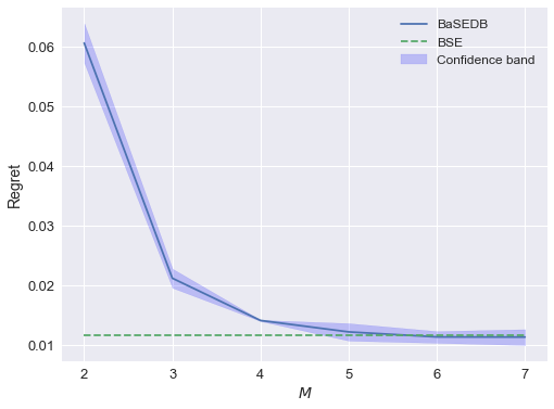
Figure 2: Regret vs. batch budget $M$.

4.3 Failure of static binning

We have seen the power of dynamic binning in solving batched nonparametric bandits by establishing its rate-optimality in minimizing regret. Now we turn to a complimentary but intriguing question: is it necessary to use dynamic binning to achieve optimal regret under the batch constraint? To formally address this question, we investigate the performance of successive elimination with static binning, i.e., Algorithm 1 with $g_{0}=g$, and $g_{1}=g_{2}=\cdots g_{M-2}=1$. Although static binning works when $M$ is large (e.g., a single choice of $g$ attains the optimal regret [48, 39] in the fully online setting), we show that it must fail when $M$ is small.

To bring the failure mode of static binning into focus, we consider the simplest scenario when $M=3$, and $\alpha=\beta=d=1$. Note that the successive elimination with static binning algorithm is parameterized by the grid choice $\Gamma=\{t_{0}=0,t_{1},t_{2},t_{3}=T\}$ and the fixed number $g$ of bins. The following theorem formalizes the failure of static binning in achieving optimal regret when $M=3$.

Theorem 3.

Consider $M=3$, and $\alpha=\beta=d=1$. For any choice of $1\leq t_{1}<t_{2}\leq T-1$, and any choice of $g$, there exists a nonparametric bandit instance in $\mathcal{F}(1,1)$ such that the resulting successive elimination with static binning algorithm $\hat{\pi}_{\mathrm{static}}$ satisfies

$$\mathbb{E}[R_{T}(\hat{\pi}_{\mathrm{static}})]\geq\tilde{C}_{1}T^{\frac{9}{19}+\kappa},$$

for some $\kappa,\tilde{C}_{1}>0$ that are independent of $T$. Here $T^{\frac{9}{19}}$ is the optimal regret achieved by BaSEDB—an successive elimination algorithm with dynamic binning.

While the formal proof is deferred to Section 6, we would like to immediately point out the intuition underlying the failure of static binning.

Necessary choice of grid $\Gamma$.

It is evident from the proof of the minimax lower bound (Theorem 1) that one needs to set $t_{1}\asymp T^{9/19}$, and $t_{2}\asymp T^{15/19}$. Otherwise, the inequality (8) guarantees the worst-case regret of $\hat{\pi}_{\mathrm{static}}$ exceeds the optimal one $T^{\frac{9}{19}}$. Consequently, we can focus on the algorithm with $t_{1}\asymp T^{9/19}$, $t_{2}\asymp T^{15/19}$, and only consider the design choice $g$.

Why fixed $g$ fails.

As a baseline for comparison, recall that in the optimal algorithm with dynamic binning, we set $g_{0}\asymp T^{3/19}$, and $g_{0}g_{1}\asymp T^{5/19}$ so that the worst case regret in three batches are all on the order of $T^{\frac{9}{19}}$. In view of this, we split the choice of $g$ into three cases.

• Suppose that $g\gg T^{3/19}$. In this case, we can construct an instance such that the reward difference only appears on an interval with length $1/z\gg 1/g$; see Figure 3. In other words, the static binning is finer than that in the reward instance. As a result, the number of pulls in the smaller bin (used by the algorithm) in the first batch is not sufficient to tell the two arms apart, that is with constant probability, arm elimination will not happen after the first batch. This necessarily yields the blowup of the regret in the second batch.

• Suppose that $g\ll T^{3/19}$. In this case, we can construct an instance such that the reward difference only appears on an interval with length $1/z\ll 1/g$; see Figure 4. In other words, the static binning is coarser than that in the reward instance. Since the aggregated reward difference on the larger bin is so small, the number of pulls in the larger bin (used by the algorithm) in the first batch is still not sufficient to result in successful arm elimination. Again, the regret on the second batch blows up.

• Suppose that $g\asymp T^{3/19}$. Since this choices matches $g_{0}$ used in the optimal dynamic binning algorithm, there is no reward instance that can blow up the regret in the first two batches. Nevertheless, since $g\ll g_{0}g_{1}\asymp T^{5/19}$, one can construct the instance similar to the previous case (i.e., Figure 4) such that the regret on the third batch blows up.

Figure 3: Instance with $g>z$. Each bin $B$ produced by $\hat{\pi}_{\mathrm{static}}$ has width $1/g$.

Figure 4: Instance with $g<z$. Each bin $B$ produced by $\hat{\pi}_{\mathrm{static}}$ has width $1/g$.

5 Regret analysis for BaSEDB

Our proof of the regret upper bound is inspired by the framework developed in [39]. Our setting presents additional technical difficulty due to the batch constraint.

We begin with introducing some useful notations. Recall the tree growing process described in section 4, where we have defined a tree $\mathcal{T}$ of depth $M$. The root (depth 0) of the tree is the whole space $\mathcal{X}$. In depth $1$, $\mathcal{X}$ has $g_{0}^{d}$ children, each of which is a bin of width $1/g_{0}$. For each bin in depth 1, it has $g_{1}^{d}$ children, each of which is a bin of width $1/(g_{0}g_{1})$. These children form the depth 2 nodes of the tree $\mathcal{T}$. We form the tree recursively until depth $M$.

For a bin $C\in\mathcal{T}$, we define its parent by $\mathsf{p}(C)=\{C^{\prime}\in\mathcal{T}:C\in\mathsf{child}(C^{\prime})\}$. Moreover, we let $\mathsf{p}^{1}(C)=\mathsf{p}(C)$ and define $\mathsf{p}^{k}(C)=\mathsf{p}(\mathsf{p}^{k-1}(C))$ for $k\geq 2$ recursively. In all, we denote by $\mathcal{P}(C)=\{C^{\prime}\in\mathcal{T}:C^{\prime}=\mathsf{p}^{k}(C)\textrm{ for some }k\geq 1\}$ all the ancestors of the bin $C$.

We also define $\mathcal{L}_{t}$ to be the set of active bins at time $t$, with the dummy case $\mathcal{L}_{0}=\{\mathcal{X}\}$. Clearly, for $1\leq t\leq t_{1}$, one has $\mathcal{L}_{1}=\mathcal{B}_{1}$, where $\mathcal{B}_{1}$ are all the bins in the first layer.

5.1 Two clean events

The regret analysis relies on two clean events. First, fix a batch $i\geq 1$, and recall $\mathcal{L}_{t_{i-1}+1}$ is the set of active bins at time $t_{i-1}+1$. We denote the random number of pulls for a bin $C\in\mathcal{L}_{t_{i-1}+1}$ within batch $i$ to be

$$m_{C,i}\coloneqq\sum_{t=t_{i-1}+1}^{t_{i}}\mathbf{1}\{X_{t}\in C\}.$$

Clearly, it has expectation

$$m_{C,i}^{\star}=\mathbb{E}[m_{C,i}]=(t_{i}-t_{i-1})\mathbb{P}_{X}(X\in C).$$

The first clean event claims that $m_{C,i}$ concentrates well around its expectation $m_{C,i}^{\star}$ uniformly over all $C\in\mathcal{T}$. We denote this event by $E$.

Lemma 2.

Suppose that $M\leq D_{1}\log(T)$ for some constant $D_{1}>0$. With probability at least $1-1/T$, for all $1\leq i\leq M$, and $C\in\mathcal{L}_{t_{i-1}+1}$, we have

$$\frac{1}{2}m_{C,i}^{\star}\leq m_{C,i}\leq\frac{3}{2}m_{C,i}^{\star}.$$

See Section 5.5.1 for the proof.

Since $M\leq D_{1}\log(T)$ by assumption, we can apply Lemma 2 to obtain

$$\mathbb{E}[R_{T}(\hat{\pi})\mathbf{1}(E^{c})]\leq T\mathbb{P}(E^{c})=1.$$

Therefore, in the remaining proof, we condition on $E$ and focus on bounding $\mathbb{E}[R_{T}(\hat{\pi})\mathbf{1}(E)]$.

The second clean event is on the elimination process. Since we use successive elimination in each bin, it is natural to expect that the optimal arm in each bin is not eliminated during the process. To mathematically specify this event, we need a few notations.

For each bin $C\in\mathcal{L}_{i}$, let $\mathcal{I}_{C}^{\prime}$ be the set of remaining arms at the end of batch $i$, i.e., after Algorithm 2 is invoked. Define

$$\bar{\mathcal{I}_{C}} =\left\{k\in\{1,-1\}:\sup_{x\in C}f^{\star}(x)-f^{(k)}(x)\leq c_{1}|C|^{\beta}\right\},$$

$$\underline{\mathcal{I}}_{C}=\left\{k\in\{1,-1\}:\sup_{x\in C}f^{\star}(x)-f^{(k)}(x)\leq c_{0}|C|^{\beta}\right\},$$

where $c_{0}=2Ld^{\beta/2}+1$ and $c_{1}=8c_{0}$. Clearly, we have

$$\underline{\mathcal{I}}_{C}\subseteq\bar{\mathcal{I}_{C}}.$$

Define a good event $\mathcal{A}_{C}=\{\underline{\mathcal{I}}_{C}\subseteq\mathcal{I}_{C}^{\prime}\subseteq\bar{\mathcal{I}_{C}}\}$, which is the event that the remaining arms in $C$ have gaps of correct order. In addition, define $\mathcal{G}_{C}=\cap_{C^{\prime}\in\mathcal{P}(C)}\mathcal{A}_{C^{\prime}}$. Recall $\mathcal{B}_{i}$ is the set of bins $C$ with $|C|=(\prod_{l=0}^{i-1}g_{l})^{-1}=w_{i}$ for $i\geq 1$.

Lemma 3.

For any $1\leq i\leq M-1$ and $C\in\mathcal{B}_{i}$, we have

$$\mathbb{P}(E\cap\mathcal{G}_{C}\cap\mathcal{A}_{C}^{c})\leq\frac{4m_{C,i}^{\star}}{T|C|^{d}}.$$

In words, Lemma 3 guarantees that $\mathcal{A}_{C}$ happens with high probability if $E$ holds and $\mathcal{A}_{C^{\prime}}$ holds for all the ancestors $C\text{\textquoteright}$ of $C$. See Section 5.5.2 for the proof.

5.2 Regret decomposition

In this section, we decompose the regret into three terms. First, for a bin $C$, we define

$$r_{T}^{\textrm{live}}(C)\coloneqq\sum_{t=1}^{T}\left(f^{\star}(X_{t})-f^{(\pi_{t}(X_{t}))}(X_{t})\right)\mathbf{1}(X_{t}\in C)\mathbf{1}(C\in\mathcal{L}_{t}).$$

In addition, define $\mathcal{J}_{t}\coloneqq\cup_{s\leq t}\mathcal{L}_{s}$ to be the set of bins that have been live up until time $t$. Correspondingly we define

$$r_{T}^{\textrm{born}}(C)\coloneqq\sum_{t=1}^{T}\left(f^{\star}(X_{t})-f^{(\pi_{t}(X_{t}))}(X_{t})\right)\mathbf{1}(X_{t}\in C)\mathbf{1}(C\in\mathcal{J}_{t}).$$

It is clear from the definition that for any $C\in\mathcal{T}$, one has

$$r_{T}^{\textrm{born}}(C) =r_{T}^{\textrm{live}}(C)+\sum_{C^{\prime}\in\mathsf{child}(C)}r_{T}^{\textrm{born}}(C^{\prime})$$

$$=r_{T}^{\textrm{born}}(C)\mathbf{1}(\mathcal{A}_{C}^{c})+r_{T}^{\textrm{live}}(C)\mathbf{1}(\mathcal{A}_{C})+\sum_{C^{\prime}\in\mathsf{child}(C)}r_{T}^{\textrm{born}}(C^{\prime})\mathbf{1}(\mathcal{A}_{C}).$$

Applying this relation recursively leads to the following regret decomposition:

$$R_{T}(\pi) =r_{T}^{\textrm{born}}(\mathcal{X})$$

$$=\underbrace{r_{T}^{\textrm{live}}(\mathcal{X})}_{=0}+\sum_{C^{\prime}\in\mathsf{child}(\mathcal{X})}r_{T}^{\textrm{born}}(C^{\prime})$$

$$=\sum_{1\leq i<M}\left(\underbrace{\sum_{C\in\mathcal{B}_{i}}r_{T}^{\textrm{born}}(C)\mathbf{1}(\mathcal{G}_{C}\cap\mathcal{A}_{C}^{c})}_{\eqqcolon U_{i}}+\underbrace{\sum_{C\in\mathcal{B}_{i}}r_{T}^{\textrm{live}}(C)\mathbf{1}(\mathcal{G}_{C}\cap\mathcal{A}_{C})}_{\eqqcolon V_{i}}\right)$$

$$\quad+\sum_{C\in\mathcal{B}_{M}}r_{T}^{\textrm{live}}(C)\mathbf{1}(\mathcal{G}_{C}),$$

where the second equality arises from the fact that $r_{T}^{\textrm{live}}(\mathcal{X})=0$. Indeed, $\mathcal{X}\notin\mathcal{L}_{t}$ for any $1\leq t\leq T$.

5.3 Controlling three terms

In what follows, we control $V_{i},U_{i}$ and the last batch separately.

5.3.1 Controlling $V_{i}$

Fix some $1\leq i\leq M-1$, and some bin $C\in\mathcal{B}_{i}$. On the event $\mathcal{G}_{C}$ we have $\mathcal{I}_{\mathsf{p}(C)}^{{}^{\prime}}\subseteq\bar{I}_{\mathsf{p}(C)}$, that is, for any $k\in\mathcal{I}_{\mathsf{p}(C)}^{{}^{\prime}}$,

$$\sup_{x\in\mathsf{p}(C)}f^{\star}(x)-f^{(k)}(x)\leq c_{1}|\mathsf{p}(C)|^{\beta}.$$

This implies that for any $x\in C$, and $k\in\mathcal{I}_{\mathsf{p}(C)}^{{}^{\prime}}$,

$$\left(f^{\star}(x)-f^{(k)}(x)\right)\bm{1}\{\mathcal{G}_{C}\}\leq c_{1}|\mathsf{p}(C)|^{\beta}\mathbf{1}(0<\left|f^{(1)}(x)-f^{(-1)}(x)\right|\leq c_{1}|\mathsf{p}(C)|^{\beta}).$$ (12)

As a result, we obtain

$$\mathbb{E}[r_{T}^{\textrm{live}}(C)\mathbf{1}(\mathcal{G}_{C}\cap\mathcal{A}_{C})]=\mathbb{E}\left[\sum_{t=1}^{T}\left(f^{\star}(X_{t})-f^{(\pi_{t}(X_{t}))}(X_{t})\right)\mathbf{1}(X_{t}\in C)\mathbf{1}(C\in\mathcal{L}_{t})\mathbf{1}(\mathcal{G}_{C}\cap\mathcal{A}_{C})\right]$$

$$\quad\overset{\mathrm{(i)}}{\leq}\mathbb{E}\left[\sum_{t=1}^{T}c_{1}|\mathsf{p}(C)|^{\beta}\mathbf{1}(0<\left|f^{(1)}(X_{t})-f^{(-1)}(X_{t})\right|\leq c_{1}|\mathsf{p}(C)|^{\beta})\mathbf{1}(X_{t}\in C,C\in\mathcal{L}_{t})\mathbf{1}(\mathcal{G}_{C}\cap\mathcal{A}_{C})\right]$$

$$\quad\overset{\mathrm{(ii)}}{\leq}c_{1}|\mathsf{p}(C)|^{\beta}\mathbb{E}\left[\sum_{t=t_{i-1}+1}^{t_{i}}\mathbf{1}(0<\left|f^{(1)}(X_{t})-f^{(-1)}(X_{t})\right|\leq c_{1}|\mathsf{p}(C)|^{\beta},X_{t}\in C)\mathbf{1}(\mathcal{G}_{C}\cap\mathcal{A}_{C})\right]$$

$$\quad\overset{\mathrm{(iii)}}{\leq}c_{1}|\mathsf{p}(C)|^{\beta}\sum_{t=t_{i-1}+1}^{t_{i}}\mathbb{P}(0<\left|f^{(1)}(X_{t})-f^{(-1)}(X_{t})\right|\leq c_{1}|\mathsf{p}(C)|^{\beta},X_{t}\in C)$$

$$\quad=c_{1}|\mathsf{p}(C)|^{\beta}(t_{i}-t_{i-1})\mathbb{P}(0<\left|f^{(1)}(X)-f^{(-1)}(X)\right|\leq c_{1}|\mathsf{p}(C)|^{\beta},X\in C).$$

Here, step (i) uses relation (12), and the fact that $\pi_{t}(X_{t})\in\mathcal{I}_{\mathsf{p}(C)}^{{}^{\prime}}$ when $X_{t}\in C$. For step (ii), if $C$ is split, then it is no longer live, so the live regret incurred on the remaining batches is zero. On the other hand, if $C$ is not split, then $|\mathcal{I}_{C}^{\prime}|=1$. Without loss of generality, assume that arm $-1$ is eliminated. Conditioned on $\mathcal{A}_{C}$, this means $-1\notin\underline{\mathcal{I}}_{C}$ and there exists $x_{0}\in C$ such that $f^{(1)}(x_{0})-f^{(-1)}(x_{0})>c_{0}|C|^{\beta}$. By the smoothness condition, having a gap at least $c_{0}|C|^{\beta}$ on a single point in $C$ implies $f^{(1)}(x)-f^{(-1)}(x)>|C|^{\beta}$ for all $x\in C$. Therefore, arm 1 which is the remaining one is the optimal arm for all $x\in C$ and would not incur any regret further. The third inequality holds since $\mathbf{1}(\mathcal{G}_{C}\cap\mathcal{A}_{C})\leq 1$.

Taking the sum over all bins in $\mathcal{B}_{i}$ and using the fact that $|\mathsf{p}(C)|=w_{i-1}$, we obtain

$$\sum_{C\in\mathcal{B}_{i}}\mathbb{E}[r_{T}^{\textrm{live}}(C)\mathbf{1}(\mathcal{G}_{C}\cap\mathcal{A}_{C})] \leq\sum_{C\in\mathcal{B}_{i}}c_{1}w_{i-1}^{\beta}(t_{i}-t_{i-1})\mathbb{P}(0<\left|f^{(1)}(X)-f^{(-1)}(X)\right|\leq c_{1}|\mathsf{p}(C)|^{\beta},X\in C)$$

$$=c_{1}w_{i-1}^{\beta}(t_{i}-t_{i-1})\sum_{C\in\mathcal{B}_{i}}\mathbb{P}(0<\left|f^{(1)}(X)-f^{(-1)}(X)\right|\leq c_{1}w_{i-1}^{\beta},X\in C).$$ (13)

Note that

$$\sum_{C\in\mathcal{B}_{i}}\mathbb{P}(0<\left|f^{(1)}(X)-f^{(-1)}(X)\right|\leq c_{1}w_{i-1}^{\beta},X\in C) =\mathbb{P}(0<\left|f^{(1)}(X)-f^{(-1)}(X)\right|\leq c_{1}w_{i-1}^{\beta})$$

$$\leq D_{0}\cdot\left[c_{1}w_{i-1}^{\beta}\right]^{\alpha},$$ (14)

where the last inequality follows from the margin condition. Combining relations (14) and (13), we reach

$$\sum_{C\in\mathcal{B}_{i}}\mathbb{E}[r_{T}^{\textrm{live}}(C)\mathbf{1}(\mathcal{G}_{C}\cap\mathcal{A}_{C})] \leq(t_{i}-t_{i-1})\cdot[c_{1}w_{i-1}^{\beta}]^{1+\alpha}\cdot D_{0}.$$

5.3.2 Controlling $U_{i}$

Fix some $1\leq i\leq M-1$, and some bin $C\in\mathcal{B}_{i}$. Again, using the definition of $\mathcal{G}_{C}$, we obtain

$$\mathbb{E}[r_{T}^{\textrm{born}}(C)\mathbf{1}(\mathcal{G}_{C}\cap\mathcal{A}_{C}^{c})] =\mathbb{E}\left[\sum_{t=1}^{T}\left(f^{\star}(X_{t})-f^{(\pi_{t}(X_{t}))}(X_{t})\right)\mathbf{1}(X_{t}\in C)\mathbf{1}(C\in\mathcal{J}_{t})\mathbf{1}(\mathcal{G}_{C}\cap\mathcal{A}_{C}^{c})\right]$$

$$\leq\mathbb{E}\left[\sum_{t=1}^{T}c_{1}|\mathsf{p}(C)|^{\beta}\mathbf{1}(0<\left|f^{(1)}(X_{t})-f^{(-1)}(X_{t})\right|\leq c_{1}|\mathsf{p}(C)|^{\beta})\mathbf{1}(X_{t}\in C,C\in\mathcal{J}_{t})\mathbf{1}(\mathcal{G}_{C}\cap\mathcal{A}_{C}^{c})\right]$$

$$\leq c_{1}|\mathsf{p}(C)|^{\beta}T\mathbb{P}(0<\left|f^{(1)}(X)-f^{(-1)}(X)\right|\leq c_{1}|\mathsf{p}(C)|^{\beta},X\in C)\mathbb{P}(\mathcal{G}_{C}\cap\mathcal{A}_{C}^{c}).$$

Apply Lemma 3 to see that

$$\mathbb{E}[r_{T}^{\textrm{born}}(C)\mathbf{1}(\mathcal{G}_{C}\cap\mathcal{A}_{C}^{c})] \leq c_{1}|\mathsf{p}(C)|^{\beta}T\mathbb{P}(0<\left|f^{(1)}(X)-f^{(-1)}(X)\right|\leq c_{1}|\mathsf{p}(C)|^{\beta},X\in C)\frac{4m_{C,i}^{\star}}{T|C|^{d}}$$

$$=c_{1}w_{i-1}^{\beta}\mathbb{P}(0<\left|f^{(1)}(X)-f^{(-1)}(X)\right|\leq c_{1}w_{i-1}^{\beta},X\in C)\frac{4(t_{i}-t_{i-1})\mathbb{P}_{X}(X\in C)}{|C|^{d}}$$

$$\leq 4\bar{c}c_{1}w_{i-1}^{\beta}\mathbb{P}(0<\left|f^{(1)}(X)-f^{(-1)}(X)\right|\leq c_{1}w_{i-1}^{\beta},X\in C)(t_{i}-t_{i-1}),$$

where we use the fact that $\mathbb{P}_{X}(X\in C)\leq\bar{c}|C|^{d}$ in the second inequality. Summing over all bins in $\mathcal{B}_{i}$, we obtain

$$\sum_{C\in\mathcal{B}_{i}}\mathbb{E}[r_{T}^{\textrm{born}}(C)\mathbf{1}(\mathcal{G}_{C}\cap\mathcal{A}_{C}^{c})] \leq 4\bar{c}c_{1}w_{i-1}^{\beta}(t_{i}-t_{i-1})\sum_{C\in\mathcal{B}_{i}}\mathbb{P}(0<\left|f^{(1)}(X)-f^{(-1)}(X)\right|\leq c_{1}w_{i-1}^{\beta},X\in C)$$

$$\leq 4\bar{c}c_{1}w_{i-1}^{\beta}(t_{i}-t_{i-1})D_{0}\cdot\left[c_{1}w_{i-1}^{\beta}\right]^{\alpha}$$

$$=4D_{0}\bar{c}(t_{i}-t_{i-1})[c_{1}w_{i-1}^{\beta}]^{1+\alpha},$$

where the second inequality reuses the bound in (14).

5.3.3 Last Batch

For $C\in\mathcal{B}_{M}$, one can similarly obtain

$$\mathbb{E}[r_{T}^{\textrm{live}}(C)\mathbf{1}(\mathcal{G}_{C})] \leq c_{1}|\mathsf{p}(C)|^{\beta}(T-t_{M-1})\mathbb{P}(0<\left|f^{(1)}(X)-f^{(-1)}(X)\right|\leq c_{1}|\mathsf{p}(C)|^{\beta},X\in C).$$

Consequently, summing over $C\in\mathcal{B}_{M}$ yields

$$\sum_{C\in\mathcal{B}_{M}}\mathbb{E}[r_{T}^{\textrm{live}}(C)\mathbf{1}(\mathcal{G}_{C})] \leq\sum_{C\in\mathcal{B}_{M}}c_{1}|\mathsf{p}(C)|^{\beta}(T-t_{M-1})\mathbb{P}(0<\left|f^{(1)}(X)-f^{(-1)}(X)\right|\leq c_{1}|\mathsf{p}(C)|^{\beta},X\in C)$$

$$\leq c_{1}w_{M-1}^{\beta}(T-t_{M-1})D_{0}\cdot\left[c_{1}w_{M-1}^{\beta}\right]^{\alpha}$$

$$=D_{0}(T-t_{M-1})[c_{1}w_{M-1}^{\beta}]^{1+\alpha}.$$

5.4 Putting things together

In sum, the total regret is bounded by

$$\mathbb{E}[R_{T}(\pi)] \leq c\left(t_{1}+\sum_{i=2}^{M-1}(t_{i}-t_{i-1})\cdot w_{i-1}^{\beta+\alpha\beta}+(T-t_{M-1})w_{M-1}^{\beta+\alpha\beta}\right),$$

where $c$ is a constant that depends on $(\alpha,\beta,D,L)$. Recall that $w_{i}=(\prod_{l=0}^{i-1}g_{l})^{-1}$, and the choices for the batch size and the split factors (11)-(10). We then obtain

$$t_{1} \lesssim T^{\frac{1-\gamma}{1-\gamma^{M}}}\log T,$$

$$(t_{i}-t_{i-1})\cdot w_{i-1}^{\beta+\alpha\beta} \lesssim T^{\frac{1-\gamma}{1-\gamma^{M}}}\log T,\qquad\text{for }2\leq i\leq M-1,$$

$$(T-t_{M-1})w_{M-1}^{\beta+\alpha\beta} \leq Tw_{M-1}^{\beta+\alpha\beta}\lesssim T^{\frac{1-\gamma}{1-\gamma^{M}}}\log T.$$

The proof is finished by combining the above three bounds.

5.5 Proofs for the clean events

We are left with proving that the two clean events happen with high probability.

5.5.1 Proof of Lemma 2

Fix the batch index $i$, and a node $C$ in layer-$i$ of the tree $\mathcal{T}$. By relation (11), we have

$$m_{C,i}^{\star} =(t_{i}-t_{i-1})\mathbb{P}_{X}(X\in C)$$

$$\asymp|C|^{-(2\beta+d)}\log(T|C|^{d})\mathbb{P}_{X}(X\in C)$$

$$\apprge|C|^{-2\beta}\overset{\mathrm{}}{\geq}g_{0}^{2\beta}\asymp(T^{\frac{1-\gamma}{1-\gamma^{M}}\cdot\frac{2\beta}{2\beta+d}}),$$

where the last step uses the fact that $\mathbb{P}_{X}(X\in C)\geq\underline{c}|C|^{d}$. Therefore, $m_{C,i}^{\star}\geq\frac{3}{4}\log(2T^{2})$ for all $i$ and $C$, as long as $T$ is sufficiently large. This allows us to invoke Chernoff’s bound to obtain that with probability at most $1/T^{2}$

$$\left|\sum\nolimits_{t=t_{i-1}+1}^{t_{i}}\mathbf{1}\{X_{t}\in C\}-m_{C,i}^{\star}\right|\geq\sqrt{3\log(2T^{2})m_{C,i}^{\star}}.$$

Denote $E^{c}=\{\exists 1\leq i\leq M,C\in\mathcal{L}_{t_{i-1}+1}\text{ such that }\mid\sum_{t=t_{i-1}+1}^{t_{i}}\mathbf{1}\{X_{t}\in C\}-m_{C,i}^{\star}\mid\geq\sqrt{3\log(2T^{2})m_{C,i}^{\star}}\}$. Applying union bound to reach

$$\mathbb{P}(E^{c}) \leq\sum_{C\in\mathcal{T}}\frac{1}{T^{2}}\overset{\mathrm{(i)}}{\leq}\frac{1}{T^{2}}\left(\sum_{i=1}^{M}(\prod_{l=0}^{i-1}g_{l})^{d}\right)\overset{\mathrm{(ii)}}{\leq}\frac{1}{T^{2}}\cdot M\cdot(\prod_{l=0}^{M-1}g_{l})^{d},$$

where step (i) sums over all possible nodes of $\mathcal{T}$ across batches, and step (ii) is due to $(\prod_{l=0}^{i-1}g_{l})^{d}\leq(\prod_{l=0}^{M-1}g_{l})^{d}$ for any $1\leq i\leq M$. Since $g_{M-1}=1$, we further obtain

$$\mathbb{P}(E^{c}) \leq\frac{1}{T^{2}}\cdot M\cdot(\prod_{l=0}^{M-2}g_{l})^{d}\overset{\mathrm{(iii)}}{\leq}\frac{1}{T^{2}}\cdot M\cdot t_{M-1}^{\frac{d}{2\beta+d}}\overset{\mathrm{(iv)}}{\leq}D_{1}\frac{1}{T^{2}}\cdot\log T\cdot T^{\frac{d}{2\beta+d}}\leq\frac{1}{T},$$

where step (iii) invokes relation (11), and step (iv) uses the assumption $M\leq D_{1}\log T$. This completes the proof.

5.5.2 Proof of Lemma 3

To simplify notation, for any event $F$, we define $\mathbb{P}^{\mathcal{G}_{C}}(F)=\mathbb{P}(E\cap\mathcal{G}_{C}\cap F)$.

Let $\mathcal{D}_{C}^{1}$ be the event that an arm $k\in\underline{\mathcal{I}}_{C}$ is eliminated at the end of batch $i$, and $\mathcal{D}_{C}^{2}$ be the event that an arm $k\notin\bar{\mathcal{I}_{C}}$ is not eliminated at the end of batch $i$. Consequently, we have

$$\mathbb{P}^{\mathcal{G}_{C}}(\mathcal{A}_{C}^{c})=\mathbb{P}^{\mathcal{G}_{C}}(\mathcal{D}_{C}^{1})+\mathbb{P}^{\mathcal{G}_{C}}((\mathcal{D}_{C}^{1})^{c}\cap\mathcal{D}_{C}^{2}).$$

Recall $U(\tau,T,C)=4\sqrt{\frac{\log(2T|C|^{d})}{\tau}}$ . By relation (11), we can write

$$m_{C,i}^{\star} =(t_{i}-t_{i-1})\mathbb{P}_{X}(X\in C)$$

$$=l_{i}|C|^{-(2\beta+d)}\log(T|C|^{d})\mathbb{P}_{X}(X\in C),$$

where $l_{i}>0$ is a constant chosen such that $U(2m_{C,i}^{\star},T,C)=2c_{0}|C|^{\beta}$. Under $E$, we have $U(m_{C,i},T,C)\leq 4c_{0}|C|^{\beta}$ because $m_{C,i}\geq\frac{1}{2}m_{C,i}^{\star}$.

1. Upper bounding $\mathbb{P}^{\mathcal{G}_{C}}(\mathcal{D}_{C}^{1})$: when $\mathcal{D}_{C}^{1}$ occurs, an arm $k\in\underline{\mathcal{I}}_{C}$ is eliminated by some $k^{\prime}\in\mathcal{I}_{\mathsf{p}(C)}^{\prime}$ at the end of batch $i$. This means $\bar{Y}_{C,i}^{(k^{\prime})}-\bar{Y}_{C,i}^{(k)}>U(m_{C,i},T,C)$. Meanwhile,

   $$\bar{f}_{C}^{(k^{\prime})}-\bar{f}_{C}^{(k)} \leq\bar{f}_{C}^{\star}-\bar{f}_{C}^{(k)}\overset{\mathrm{(i)}}{\leq}c_{0}|C|^{\beta}\leq\frac{1}{2}U(2m_{C,i}^{\star},T,C),$$

   where step (i) uses the definition of $\underline{\mathcal{I}}_{C}$. Consequently, ${|\bar{Y}_{C,i}^{(k^{\prime})}-\bar{f}_{C}^{(k^{\prime})}|\leq U(m_{C,i},T,C)/4}$ and $|\bar{Y}_{C,i}^{(k)}-\bar{f}_{C}^{(k)}|\leq U(m_{C,i},T,C)/4$ cannot hold simultaneously. Otherwise, this would contradict with $\bar{Y}_{C,i}^{(k^{\prime})}-\bar{Y}_{C,i}^{(k)}>U(m_{C,i},T,C)$ because $m_{C,i}\leq 2m_{C,i}^{\star}$ under $E$. Therefore,

   $$\mathbb{P}^{\mathcal{G}_{C}}(\mathcal{D}_{C}^{1}) \leq\mathbb{P}\left\{\exists k\in\mathcal{I}_{\mathsf{p}(C)}^{\prime},m_{C,i}\leq 2m_{C,i}^{\star}:|\bar{Y}_{C,i}^{(k)}-\bar{f}_{C}^{(k)}|\geq\frac{1}{4}U(m_{C,i},T,C)\right\}.$$

2. Upper bounding $\mathbb{P}^{\mathcal{G}_{C}}((\mathcal{D}_{C}^{1})^{c}\cap\mathcal{D}_{C}^{2})$: when $(\mathcal{D}_{C}^{1})^{c}\cap\mathcal{D}_{C}^{2}$ happens, no arm in $\underline{\mathcal{I}}_{C}$ is eliminated while some $k\notin\bar{\mathcal{I}_{C}}$ remains in the active arm set. By definition, there exists $x^{(k)}$ such that ${f^{\star}(x^{(k)})-f^{(k)}(x^{(k)})>8c_{0}|C|^{\beta}}.$ Let $\eta(k)$ be any arm that satisfies $f^{\star}(x^{(k)})=f^{(\eta(k))}(x^{(k)})$, and one can easily verify $\eta(k)\in\underline{\mathcal{I}}_{C}$. Since $k$ is not eliminated, we have $\bar{Y}_{C,i}^{(\eta(k))}-\bar{Y}_{C,i}^{(k)}\leq U(m_{C,i},T,C)$. On the other hand,

   $$\bar{f}_{C}^{(\eta(k))} \overset{(\mathrm{iii})}{\geq}f^{(\eta(k))}(x^{(k)})-c_{0}|C|^{\beta}$$

   $$\geq f^{(k)}(x^{(k)})+8c_{0}|C|^{\beta}-c_{0}|C|^{\beta}$$

   $$=f^{(k)}(x^{(k)})+7c_{0}|C|^{\beta}$$

   $$\overset{(\mathrm{iv})}{\geq}\bar{f}_{C}^{(k)}+6c_{0}|C|^{\beta}\geq\bar{f}_{C}^{(k)}+\frac{3}{2}U(m_{C,i},T,C),$$ (15)

   where steps (iii) and (iv) use Lemma 5. Inequality (15) together with the fact that $\bar{Y}_{C,i}^{(\eta(k))}-\bar{Y}_{C,i}^{(k)}\leq U(m_{C,i},T,C)$ imply $|\bar{Y}_{C,i}^{(k_{0})}-\bar{f}_{C}^{(k_{0})}|\geq U(m_{C,i},T,C)/4$ for either $k_{0}=k$ or $k_{0}=\eta(k)$. Consequently,

   $$\mathbb{P}^{\mathcal{G}_{C}}((\mathcal{D}_{C}^{1})^{c}\cap\mathcal{D}_{C}^{2}) \leq\mathbb{P}\left\{\exists k\in\mathcal{I}_{\mathsf{p}(C)}^{\prime},m_{C,i}\leq 2m_{C,i}^{\star}:|\bar{Y}_{C,i}^{(k)}-\bar{f}_{C}^{(k)}|\geq\frac{1}{4}U(m_{C,i},T,C)\right\}.$$

Combining the two parts we obtain

$$\mathbb{P}^{\mathcal{G}_{C}}(\mathcal{A}_{C}^{c}) =\mathbb{P}^{\mathcal{G}_{C}}(\mathcal{D}_{C}^{1})+\mathbb{P}^{\mathcal{G}_{C}}((\mathcal{D}_{C}^{1})^{c}\cap\mathcal{D}_{C}^{2})$$

$$\leq 2\cdot\mathbb{P}\left\{\exists k\in\mathcal{I}_{\mathsf{p}(C)}^{\prime},m_{C,i}\leq 2m_{C,i}^{\star}:|\bar{Y}_{C,i}^{(k)}-\bar{f}_{C}^{(k)}|\geq\frac{1}{4}U(m_{C,i},T,C)\right\}$$

$$\leq\frac{4m_{C,i}^{\star}}{T|C|^{d}},$$

where the last inequality applies Lemma 4.

5.5.3 Auxiliary lemmas

Lemma 4.

For any $1\leq i\leq M-1$ and $C\in\mathcal{B}_{i}$, one has

$$\mathbb{P}\left\{\exists k\in\mathcal{I}_{\mathsf{p}(C)}^{\prime},m_{C,i}\leq 2m_{C,i}^{\star}:|\bar{Y}_{C,i}^{(k)}-\bar{f}_{C}^{(k)}|\geq\frac{1}{4}U(m_{C,i},T,C)\right\}\leq\frac{2m_{C,i}^{\star}}{T|C|^{d}}.$$

Proof.

Recall in Algorithm 1 we pull each arm in a round-robin fashion within a bin during batch $i$. Fix $\tau>0$. Let $\bar{Y}_{\tau}^{(k)}=\sum_{j=1}^{\tau}Y_{j}^{(k)}/\tau$ where $Y_{j}^{(k)}$’s are i.i.d. random variables with $Y_{j}^{(k)}\in[0,1]$ and $\mathbb{E}[Y_{j}^{(k)}]=\bar{f}_{C}^{(k)}$. By Hoeffding’s inequality, with probability $1/(T|C|^{d})$, we have

$$|\bar{Y}_{\tau}^{(k)}-\bar{f}_{C}^{(k)}|\geq\sqrt{\frac{\log(2T|C|^{d})}{2\tau}}.$$

Applying union bound to get

$$\mathbb{P}\left\{\exists k\in\mathcal{I}_{\mathsf{p}(C)},0\leq\tau\leq m_{C,i}^{\star}:|\bar{Y}_{\tau}^{(k)}-\bar{f}_{C}^{(k)}|\geq\sqrt{\frac{\log(2T|C|^{d})}{2\tau}}\right\}\leq\frac{2m_{C,i}^{\star}}{T|C|^{d}},$$

which completes the proof. ∎

Lemma 5.

Fix $k\in\{1,-1\}$ and $C\in\mathcal{T}$, for any $x\in C$, one has

$$|\bar{f}_{C}^{(k)}-f^{(k)}(x)|\leq c_{0}|C|^{\beta},$$

where $c_{0}=2Ld^{\beta/2}+1$.

Proof.

For notation simplicity, we write $f$ for $f^{(k)}$ in the following proof. By definition,

$$|\bar{f}_{C}-f(x)| =|\frac{1}{\mathbb{P}(C)}\int_{C}(f(y)-f(x))\mathsf{d}\mathbb{P}(y)|$$

$$\leq\frac{1}{\mathbb{P}(C)}\int_{C}|f(y)-f(x)|\mathsf{d}\mathbb{P}(y)$$

$$\leq\frac{1}{\mathbb{P}(C)}\int_{C}L\|x-y\|_{2}^{\beta}\mathsf{d}\mathbb{P}(y),$$

where the first inequality uses the triangle inequality, and the second inequality is due to the smoothness condition. Since $x\in C$, we further have

$$|\bar{f}_{C}-f(x)| \leq\frac{1}{\mathbb{P}(C)}\int_{C}L\|x-y\|_{2}^{\beta}\mathsf{d}\mathbb{P}(y)$$

$$\leq\frac{1}{\mathbb{P}(C)}\int_{C}Ld^{\beta/2}|C|^{\beta}\mathsf{d}\mathbb{P}(y)$$

$$\leq c_{0}|C|^{\beta}.$$

This completes the proof. ∎

6 Proof of suboptimality of static binning

As we argued after the statement of Theorem 3, one needs to set $t_{1}\asymp T^{9/19}$, and $t_{2}\asymp T^{15/19}$. Therefore, throughout the proof, we assume this is true and only focus on the number $g$ of bins.

To construct a hard instance, we partition $[0,1]$ into $z$ bins with equal width. Denote the bins by $C_{j}$ for $j=1,...,z$, and let $q_{j}$ be the center of $C_{j}$. Define a function $\phi:[0,1]\mapsto\mathbb{R}$ as $\phi(x)=(1-|x|)\mathbf{1}\{|x|\leq 1\}.$ Correspondingly define a function $\varphi_{j}:[0,1]\mapsto\mathbb{R}$ as $\varphi_{j}(x)=D_{\phi}z^{-1}\phi(2z(x-q_{j}))\mathbf{1}\{x\in C_{j}\},$ where $D_{\phi}=\min(2^{-1}L,1/4)$. Define a function $f:[0,1]\mapsto\mathbb{R}$:

$$f(x)=\frac{1}{2}+\varphi_{1}(x).$$

The problem instance of interest is $v=(f^{(1)}(x)=f(x),f^{(-1)}(x)=\frac{1}{2})$. It is easy to verify $v\in\mathcal{F}(1,1).$ Throughout the proof, we condition on the event $E$ specified by Lemma 2, which says the number of samples allocated to a bin concentrates well around its expectation. We will show even under this good event, there exists a choice of $z$ that makes successive elimination fail to remove the suboptimal arms at the end of a batch with constant probability.

6.1 A helper lemma

We begin with presenting a helper lemma that will be used extensively in the later part of the proof. The claim is intuitive: if the sample size is small, it is not sufficient to tell apart two Bernoulli distributions with similar means. Then, in our context, arm elimination will not occur.

Lemma 6.

Assume $m_{B,i}\leq 2m_{B,i}^{\star}$. For any $B\subseteq[0,1]$ and $i\in\{1,2\}$. If $\bar{f}_{B}^{(1)}-\bar{f}_{B}^{(-1)}\leq\delta\leq 1/\sqrt{m_{B,i}^{\star}}$ for some $\delta>0$ , then

$$\mathbb{P}\left(\bar{Y}_{B,i}^{(1)}-\bar{Y}_{B,i}^{(-1)}>U(m_{B,i},T,B)\right)\leq\frac{t_{i}}{T}.$$

Proof.

Fix $0<\tau\leq m_{B,i}^{\star}$. Let $\bar{Y}_{\tau}^{(k)}=\sum_{l=1}^{\tau}Y_{l}^{(k)}/\tau$ where $Y_{l}^{(k)}$’s are i.i.d. random variables with $Y_{l}^{(k)}\in[0,1]$ and $\mathbb{E}[Y_{l}^{(k)}]=\bar{f}_{B}^{(k)}$ for $k\in\{1,-1\}$. Recall $U(\tau,T,B)=4\sqrt{\frac{\log(2T|B|)}{\tau}}$. Then,

$$\mathbb{P}\left(\bar{Y}_{\tau}^{(1)}-\bar{Y}_{\tau}^{(-1)}>U(2\tau,T,B)\right) \overset{\mathrm{(i)}}{\leq}\mathbb{P}\left(\bar{Y}_{\tau}^{(1)}-\bar{Y}_{\tau}^{(-1)}>\delta+\sqrt{\frac{\log(2T/g)}{2\tau}}\right)$$

$$\overset{\mathrm{(ii)}}{\leq}\mathbb{P}\left(\bar{Y}_{\tau}^{(1)}-\bar{Y}_{\tau}^{(-1)}>\bar{f}_{B}^{(1)}-\bar{f}_{B}^{(-1)}+\sqrt{\frac{\log(2T/g)}{2\tau}}\right)$$

$$\overset{\mathrm{(iii)}}{\leq}\frac{g}{T},$$

where step (i) is because $\delta\leq 1/\sqrt{m_{B,i}^{\star}}\leq 1/\sqrt{\tau}$, step (ii) is due to $\bar{f}_{B}^{(1)}-\bar{f}_{B}^{(-1)}\leq\delta$, and step (iii) uses Hoeffding’s inequality. Applying union bound to get

$$\mathbb{P}\left(\exists 0<\tau\leq m_{B,i}^{\star}:\bar{Y}_{\tau}^{(1)}-\bar{Y}_{\tau}^{(-1)}>U(2\tau,T,B)\right)\leq\frac{m_{B,i}^{\star}g}{T}\leq\frac{t_{i}}{T}.$$

This finishes the proof. ∎

6.2 Three failure cases for $g$

Fix some small constant $\varepsilon>0$ to be specified later. From now on, we use $\hat{\pi}$ to denote $\hat{\pi}_{\mathrm{static}}$ for simplicity. We split the proof into three cases: (1) $g\geq T^{3/19+\varepsilon}$; (2) $g\leq T^{3/19-\varepsilon}$; (3) and $g\in(T^{3/19-\varepsilon},T^{3/19+\varepsilon})$.

Case 1: $g\geq T^{3/19+\varepsilon}$.

Set $z=T^{3/19-\varepsilon/2}$. Assume without loss of generality that $g=H\cdot z$ for some $H\geq 4$; see Figure 3 for an illustration of the instance. Suppose $C_{1}=\cup_{l=1}^{H}B_{l}$, where $B_{l}$’s are the bins produced by $\hat{\pi}$ that lie in $C_{1}$. It is clear that

$$\mathbb{E}[R_{T}(\hat{\pi})] \overset{\mathrm{(i)}}{\geq}\mathbb{E}\left[\sum_{t=t_{1}+1}^{t_{2}}\left(f^{\star}(X_{t})-f^{\hat{\pi}_{t}(X_{t})}(X_{t})\right)\right]$$

$$\overset{\mathrm{(ii)}}{=}\mathbb{E}\left[\sum_{t=t_{1}+1}^{t_{2}}\left(f^{\star}(X_{t})-f^{\hat{\pi}_{t}(X_{t})}(X_{t})\right)\mathbf{1}\{X_{t}\in C_{1}\}\right]$$

$$\overset{\mathrm{(iii)}}{\geq}\sum_{t=t_{1}+1}^{t_{2}}\sum_{l=H/4}^{3H/4}\mathbb{E}\left[\left(f^{\star}(X_{t})-f^{\hat{\pi}_{t}(X_{t})}(X_{t})\right)\mathbf{1}\{X_{t}\in B_{l}\}\right],$$ (16)

where step (i) is because the total regret is greater than the regret incurred during the second batch, step (ii) uses the fact that under the instance $v$, the mean rewards of the two arms differ only in $C_{1}$, and step (iii) arises since $C_{1}=\cup_{l=1}^{H}B_{l}$. Now we turn to lower bounding $\mathbb{E}\left[\left(f^{\star}(X_{t})-f^{\hat{\pi}_{t}(X_{t})}(X_{t})\right)\mathbf{1}\{X_{t}\in B_{l}\}\right]$ for each $H/4\leq l\leq 3H/4$.

Consider any such $B_{l}$. We drop the subscripts and write $B$ instead for simplicity. By the design of $v$, we have $\bar{f}_{B}^{(1)}-\bar{f}_{B}^{(-1)}\leq D_{\phi}z^{-1}=\delta$, which obeys $D_{\phi}z^{-1}\leq 1/\sqrt{m_{B,1}^{\star}}$—a consequence of the choice of $z$. Additionally, we have $m_{B,1}\leq 2m_{B,1}^{\star}$ under $E$. Therefore, we can invoke Lemma 6 to obtain

$$\mathbb{P}\left(\bar{Y}_{B,1}^{(1)}-\bar{Y}_{B,1}^{(-1)}>U(m_{B,1},T,B)\right)\leq\frac{t_{1}}{T}\leq\frac{1}{2}.$$

In words, with probability exceeding $1/2$, no elimination will happen for the bin $B$. As a result, we obtain

$$\mathbb{E}[R_{T}(\hat{\pi})] \geq\sum_{t=t_{1}+1}^{t_{2}}\sum_{l=H/4}^{3H/4}\mathbb{E}\left[\left(f^{\star}(X_{t})-f^{\hat{\pi}_{t}(X_{t})}(X_{t})\right)\mathbf{1}\{X_{t}\in B_{l}\}\right]$$

$$\gtrsim H\cdot\frac{t_{2}}{g}\cdot z^{-1}\asymp\frac{t_{2}}{z^{2}}=T^{\frac{9}{19}+\epsilon},$$

where we have used the choice of $z$. So Theorem (3) holds with $\kappa=\epsilon$.

Case 2: $g\leq T^{3/19-\varepsilon}$.

Set $z=T^{3/19-\varepsilon/8}$. We have $g<z$ and there exists $H>1$ such that $z=H\cdot g$; see Figure 4 for an illustration of the instance. Let $B$ be the bin produced by $\hat{\pi}$ such that $C_{1}\subset B$. By the design of $v$, we have

$$\bar{f}_{B}^{(1)}-\bar{f}_{B}^{(-1)}\leq\frac{1}{H}(1/2+D_{\phi}z^{-1})+(1-\frac{1}{H})\frac{1}{2}-\frac{1}{2}=\frac{D_{\phi}z^{-1}}{H}.$$

Let $\delta=\frac{D_{\phi}z^{-1}}{H}$, we have $\delta\leq 1/\sqrt{m_{B,1}^{\star}}$ due to our choice of $z$. Additionally, we have $m_{B,1}\leq 2m_{B,1}^{\star}$ under $E$. Therefore, we can invoke Lemma 6 to obtain

$$\mathbb{P}\left(\bar{Y}_{B,1}^{(1)}-\bar{Y}_{B,1}^{(-1)}>U(m_{B,1},T,B)\right)\leq\frac{t_{1}}{T}\leq\frac{1}{2}.$$

Thus, with probability exceeding $1/2$, the suboptimal arm is not eliminated in $B$. Similar to the previous case, we obtain

$$\mathbb{E}[R_{T}(\hat{\pi})] \overset{\mathrm{}}{\geq}\mathbb{E}\left[\sum_{t=t_{1}+1}^{t_{2}}\left(f^{\star}(X_{t})-f^{\hat{\pi}_{t}(X_{t})}(X_{t})\right)\right]$$

$$\overset{\mathrm{}}{=}\mathbb{E}\left[\sum_{t=t_{1}+1}^{t_{2}}\left(f^{\star}(X_{t})-f^{\hat{\pi}_{t}(X_{t})}(X_{t})\right)\mathbf{1}\{X_{t}\in C_{1}\}\right]$$

$$\apprge\frac{t_{2}}{z^{2}}\overset{\mathrm{}}{=}T^{\frac{9}{19}+\frac{\epsilon}{4}}.$$

So Theorem (3) holds with $\kappa=\epsilon/4$.

Case 3: $g\in(T^{3/19-\varepsilon},T^{3/19+\varepsilon})$.

Set $z\asymp T^{1/4}$. We then have $g<z$, as long as $\varepsilon\leq 1/19$. And there exists $H>1$ such that $z=H\cdot g$; see Figure 4 for an illustration of the instance. Let $B$ be the bin produced by $\hat{\pi}$ such that $C_{1}\subset B$. By the design of $v$, we have

$$\bar{f}_{B}^{(1)}-\bar{f}_{B}^{(-1)}\leq\frac{1}{H}(1/2+D_{\phi}z^{-1})+(1-\frac{1}{H})\frac{1}{2}-\frac{1}{2}=\frac{D_{\phi}z^{-1}}{H}.$$

Let $\delta=\frac{D_{\phi}z^{-1}}{H}$, we have $\delta\leq 1/\sqrt{m_{B,1}^{\star}}$ due to our choice of $z$. Additionally, we have $m_{B,1}\leq 2m_{B,1}^{\star}$ under $E$. Therefore, we can invoke Lemma 6 to obtain

$$\mathbb{P}\left(\bar{Y}_{B,1}^{(1)}-\bar{Y}_{B,1}^{(-1)}>U(m_{B,1},T,B)\right)\leq\frac{t_{1}}{T}\leq\frac{1}{4}.$$

This means with probability at least $3/4$, arm elimination does not occur in $B$ after the first batch. Moreover, since $\delta\leq 1/\sqrt{m_{B,2}^{\star}}$ by the choice of $z$, and $m_{B,2}\leq 2m_{B,2}^{\star}$ under $E$, we can apply Lemma 6 again to get

$$\mathbb{P}\left(\bar{Y}_{B,2}^{(1)}-\bar{Y}_{B,2}^{(-1)}>U(m_{B,2},T,B)\right)\leq\frac{t_{2}}{T}\leq\frac{1}{4}.$$

In all, with probability at least $1/2$, arm elimination does not occur in $B$ after the second batch. Similar to before, we reach the conclusion that

$$\mathbb{E}[R_{T}(\hat{\pi})] \overset{\mathrm{}}{\geq}\mathbb{E}\left[\sum_{t=t_{2}+1}^{T}\left(f^{\star}(X_{t})-f^{\hat{\pi}_{t}(X_{t})}(X_{t})\right)\right]$$

$$\overset{\mathrm{}}{=}\mathbb{E}\left[\sum_{t=t_{2}+1}^{T}(f^{\star}(X_{t})-f^{\hat{\pi}_{t}(X_{t})}(X_{t}))\mathbf{1}\{X_{t}\in C_{1}\}\right]$$

$$\overset{\mathrm{}}{\gtrsim}\frac{T}{z^{2}}\overset{\mathrm{}}{=}T^{\frac{1}{2}}.$$

We see that Theorem (3) holds with $\kappa=1/38$.

7 Discussion

In this paper, we characterize the fundamental limits of batch learning in nonparametric contextual bandits. In particular, our optimal batch learning algorithm (i.e., Algorithm 1) is able to match the optimal regret in the fully online setting with only $O(\log\log T)$ policy updates. Our work open a few interesting avenues to explore in the future.

Extensions to multiple arms.

With slight modification, our algorithm works for nonparametric contextual bandits with more than two arms. However, it remains unclear what the fundamental limits of batch learning are in this multi-armed case.

Improving the log factor.

Comparing the upper and lower bounds, it is evident that Algorithm 1 is near-optimal up to log factors. It is certainly interesting to improve this log factor, either by strengthening the lower bound, or making the upper bound more efficient.

Adapting to smoothness and margin parameters.

In practice, we do not always know the smoothness and the margin parameters. Can one develop a batch learning algorithm that can adapt to these unknown parameters? This question is intriguing because in the fully online setting, a similar adaptively binned successive elimination algorithm was proposed in [39] with the sole purpose of adapting to the margin parameter.

Acknowledgements

CM is partially supported by the National Science Foundation via grant DMS-2311127.

References

- [1] Yasin Abbasi-Yadkori, Dávid Pál, and Csaba Szepesvári. Improved algorithms for linear stochastic bandits. Advances in neural information processing systems, 24, 2011.
- [2] Sakshi Arya and Yuhong Yang. Randomized allocation with nonparametric estimation for contextual multi-armed bandits with delayed rewards. Statistics & Probability Letters, 164:108818, 2020.
- [3] Jean-Yves Audibert and Alexandre B Tsybakov. Fast learning rates for plug-in classifiers. The Annals of Statistics, 35(2):608–633, 2007.
- [4] Peter Auer. Using confidence bounds for exploitation-exploration trade-offs. Journal of Machine Learning Research, 3(Nov):397–422, 2002.
- [5] Yu Bai, Tengyang Xie, Nan Jiang, and Yu-Xiang Wang. Provably efficient q-learning with low switching cost. Advances in Neural Information Processing Systems, 32, 2019.
- [6] Hamsa Bastani and Mohsen Bayati. Online decision making with high-dimensional covariates. Operations Research, 68(1):276–294, 2020.
- [7] Hamsa Bastani, Mohsen Bayati, and Khashayar Khosravi. Mostly exploration-free algorithms for contextual bandits. Management Science, 67(3):1329–1349, 2021.
- [8] Dimitris Bertsimas and Adam J Mersereau. A learning approach for interactive marketing to a customer segment. Operations Research, 55(6):1120–1135, 2007.
- [9] Moise Blanchard, Steve Hanneke, and Patrick Jaillet. Non-stationary contextual bandits and universal learning. arXiv preprint arXiv:2302.07186, 2023.
- [10] Changxiao Cai, T Tony Cai, and Hongzhe Li. Transfer learning for contextual multi-armed bandits. arXiv preprint arXiv:2211.12612, 2022.
- [11] T Tony Cai and Hongming Pu. Stochastic continuum-armed bandits with additive models: Minimax regrets and adaptive algorithm. The Annals of Statistics, 50(4):2179–2204, 2022.
- [12] Nicolo Cesa-Bianchi, Ofer Dekel, and Ohad Shamir. Online learning with switching costs and other adaptive adversaries. Advances in Neural Information Processing Systems, 26, 2013.
- [13] Olivier Chapelle. Modeling delayed feedback in display advertising. In Proceedings of the 20th ACM SIGKDD international conference on Knowledge discovery and data mining, pages 1097–1105, 2014.
- [14] Olivier Chapelle and Lihong Li. An empirical evaluation of thompson sampling. Advances in neural information processing systems, 24, 2011.
- [15] Stephen E Chick and Noah Gans. Economic analysis of simulation selection problems. Management Science, 55(3):421–437, 2009.
- [16] Eyal Even-Dar, Shie Mannor, Yishay Mansour, and Sridhar Mahadevan. Action elimination and stopping conditions for the multi-armed bandit and reinforcement learning problems. Journal of machine learning research, 7(6):1079–1105, 2006.
- [17] Jianqing Fan, Zhaoran Wang, Zhuoran Yang, and Chenlu Ye. Provably efficient high-dimensional bandit learning with batched feedbacks. arXiv preprint arXiv:2311.13180, 2023.
- [18] Yasong Feng, Zengfeng Huang, and Tianyu Wang. Lipschitz bandits with batched feedback. Advances in Neural Information Processing Systems, 35:19836–19848, 2022.
- [19] Manegueu Anne Gael, Claire Vernade, Alexandra Carpentier, and Michal Valko. Stochastic bandits with arm-dependent delays. In International Conference on Machine Learning, pages 3348–3356. PMLR, 2020.
- [20] Minbo Gao, Tianle Xie, Simon S Du, and Lin F Yang. A provably efficient algorithm for linear markov decision process with low switching cost. arXiv preprint arXiv:2101.00494, 2021.
- [21] Zijun Gao, Yanjun Han, Zhimei Ren, and Zhengqing Zhou. Batched multi-armed bandits problem. Advances in Neural Information Processing Systems, 32, 2019.
- [22] Alexander Goldenshluger and Assaf Zeevi. Woodroofe’s one-armed bandit problem revisited. The Annals of Applied Probability, 19(4):1603–1633, 2009.
- [23] Alexander Goldenshluger and Assaf Zeevi. A linear response bandit problem. Stochastic Systems, 3(1):230–261, 2013.
- [24] Melody Guan and Heinrich Jiang. Nonparametric stochastic contextual bandits. In Proceedings of the AAAI Conference on Artificial Intelligence, volume 32, 2018.
- [25] Yonatan Gur, Ahmadreza Momeni, and Stefan Wager. Smoothness-adaptive contextual bandits. Operations Research, 70(6):3198–3216, 2022.
- [26] Yanjun Han, Zhengqing Zhou, Zhengyuan Zhou, Jose Blanchet, Peter W Glynn, and Yinyu Ye. Sequential batch learning in finite-action linear contextual bandits. arXiv preprint arXiv:2004.06321, 2020.
- [27] Yichun Hu, Nathan Kallus, and Xiaojie Mao. Smooth contextual bandits: Bridging the parametric and nondifferentiable regret regimes. Operations Research, 70(6):3261–3281, 2022.
- [28] Cem Kalkanli and Ayfer Ozgur. Batched thompson sampling. Advances in Neural Information Processing Systems, 34:29984–29994, 2021.
- [29] Amin Karbasi, Vahab Mirrokni, and Mohammad Shadravan. Parallelizing thompson sampling. Advances in Neural Information Processing Systems, 34:10535–10548, 2021.
- [30] Edward S Kim, Roy S Herbst, Ignacio I Wistuba, J Jack Lee, George R Blumenschein Jr, Anne Tsao, David J Stewart, Marshall E Hicks, Jeremy Erasmus Jr, Sanjay Gupta, et al. The battle trial: personalizing therapy for lung cancer. Cancer discovery, 1(1):44–53, 2011.
- [31] Aniket Kittur, Ed H Chi, and Bongwon Suh. Crowdsourcing user studies with mechanical turk. In Proceedings of the SIGCHI conference on human factors in computing systems, pages 453–456, 2008.
- [32] Anders Bredahl Kock and Martin Thyrsgaard. Optimal sequential treatment allocation. arXiv preprint arXiv:1705.09952, 2017.
- [33] Akshay Krishnamurthy, John Langford, Aleksandrs Slivkins, and Chicheng Zhang. Contextual bandits with continuous actions: Smoothing, zooming, and adapting. The Journal of Machine Learning Research, 21(1):5402–5446, 2020.
- [34] Tor Lattimore and Csaba Szepesvári. Bandit algorithms. Cambridge University Press, 2020.
- [35] Lihong Li, Wei Chu, John Langford, and Robert E Schapire. A contextual-bandit approach to personalized news article recommendation. In Proceedings of the 19th international conference on World wide web, pages 661–670, 2010.
- [36] Andrea Locatelli and Alexandra Carpentier. Adaptivity to smoothness in x-armed bandits. In Conference on Learning Theory, pages 1463–1492. PMLR, 2018.
- [37] Tyler Lu, Dávid Pál, and Martin Pál. Showing relevant ads via context multi-armed bandits. In Proceedings of AISTATS, 2009.
- [38] Enno Mammen and Alexandre B Tsybakov. Smooth discrimination analysis. The Annals of Statistics, 27(6):1808–1829, 1999.
- [39] Vianney Perchet and Philippe Rigollet. The multi-armed bandit problem with covariates. Ann. Statist., 41(2):693–721, 2013.
- [40] Vianney Perchet, Philippe Rigollet, Sylvain Chassang, and Erik Snowberg. Batched bandit problems. Ann. Statist., 44(2):660–681, 2016.
- [41] Wei Qian, Ching-Kang Ing, and Ji Liu. Adaptive algorithm for multi-armed bandit problem with high-dimensional covariates. Journal of the American Statistical Association, pages 1–13, 2023.
- [42] Wei Qian and Yuhong Yang. Kernel estimation and model combination in a bandit problem with covariates. Journal of Machine Learning Research, 17(149), 2016.
- [43] Wei Qian and Yuhong Yang. Randomized allocation with arm elimination in a bandit problem with covariates. Electronic Journal of Statistics, 10(1):242–270, 2016.
- [44] Dan Qiao, Ming Yin, Ming Min, and Yu-Xiang Wang. Sample-efficient reinforcement learning with loglog (t) switching cost. In International Conference on Machine Learning, pages 18031–18061. PMLR, 2022.
- [45] Henry Reeve, Joe Mellor, and Gavin Brown. The k-nearest neighbour ucb algorithm for multi-armed bandits with covariates. In Algorithmic Learning Theory, pages 725–752. PMLR, 2018.
- [46] Zhimei Ren and Zhengyuan Zhou. Dynamic batch learning in high-dimensional sparse linear contextual bandits. Management Science, 2023.
- [47] Zhimei Ren, Zhengyuan Zhou, and Jayant R Kalagnanam. Batched learning in generalized linear contextual bandits with general decision sets. IEEE Control Systems Letters, 6:37–42, 2020.
- [48] Philippe Rigollet and Assaf Zeevi. Nonparametric bandits with covariates. arXiv preprint arXiv:1003.1630, 2010.
- [49] Herbert E. Robbins. Some aspects of the sequential design of experiments. Bulletin of the American Mathematical Society, 58:527–535, 1952.
- [50] Eric M Schwartz, Eric T Bradlow, and Peter S Fader. Customer acquisition via display advertising using multi-armed bandit experiments. Marketing Science, 36(4):500–522, 2017.
- [51] Joe Suk and Samory Kpotufe. Tracking most significant shifts in nonparametric contextual bandits. arXiv preprint arXiv:2307.05341, 2023.
- [52] Joseph Suk and Samory Kpotufe. Self-tuning bandits over unknown covariate-shifts. In Algorithmic Learning Theory, pages 1114–1156. PMLR, 2021.
- [53] Ambuj Tewari and Susan A Murphy. From ads to interventions: Contextual bandits in mobile health. In Mobile Health, pages 495–517. Springer, 2017.
- [54] Alexander B Tsybakov. Optimal aggregation of classifiers in statistical learning. The Annals of Statistics, 32(1):135–166, 2004.
- [55] Claire Vernade, Olivier Cappé, and Vianney Perchet. Stochastic bandit models for delayed conversions. arXiv preprint arXiv:1706.09186, 2017.
- [56] Chi-Hua Wang and Guang Cheng. Online batch decision-making with high-dimensional covariates. In International Conference on Artificial Intelligence and Statistics, pages 3848–3857. PMLR, 2020.
- [57] Tianhao Wang, Dongruo Zhou, and Quanquan Gu. Provably efficient reinforcement learning with linear function approximation under adaptivity constraints. Advances in Neural Information Processing Systems, 34:13524–13536, 2021.
- [58] Michael Woodroofe. A one-armed bandit problem with a concomitant variable. Journal of the American Statistical Association, 74(368):799–806, 1979.
- [59] Yuhong Yang and Dan Zhu. Randomized allocation with nonparametric estimation for a multi-armed bandit problem with covariates. Ann. Statist., 30(1):100–121, 2002.
- [60] Kelly Zhang, Lucas Janson, and Susan Murphy. Inference for batched bandits. Advances in neural information processing systems, 33:9818–9829, 2020.
- [61] Zihan Zhang, Yuan Zhou, and Xiangyang Ji. Almost optimal model-free reinforcement learning via reference-advantage decomposition. Advances in Neural Information Processing Systems, 33:15198–15207, 2020.
- [62] Zhijin Zhou, Yingfei Wang, Hamed Mamani, and David G Coffey. How do tumor cytogenetics inform cancer treatments? dynamic risk stratification and precision medicine using multi-armed bandits. Dynamic Risk Stratification and Precision Medicine Using Multi-armed Bandits (June 17, 2019).