Abstract

This paper revisits the convergence of Stochastic Mirror Descent (SMD) in the contemporary nonconvex optimization setting. Existing results for batch-free nonconvex SMD restrict the choice of the distance generating function (DGF) to be differentiable with Lipschitz continuous gradients, thereby excluding important setups such as Shannon entropy. In this work, we present a new convergence analysis of nonconvex SMD supporting general DGF, that overcomes the above limitations and relies solely on the standard assumptions. Moreover, our convergence is established with respect to the Bregman Forward-Backward envelope, which is a stronger measure than the commonly used squared norm of gradient mapping. We further extend our results to guarantee high probability convergence under sub-Gaussian noise and global convergence under the generalized Bregman Proximal Polyak-Łojasiewicz condition. Additionally, we illustrate the advantages of our improved SMD theory in various nonconvex machine learning tasks by harnessing nonsmooth DGFs. Notably, in the context of nonconvex differentially private (DP) learning, our theory yields a simple algorithm with a (nearly) dimension-independent utility bound. For the problem of training linear neural networks, we develop provably convergent stochastic algorithms.

1 INTRODUCTION

We consider stochastic composite optimization

$$\min_{x\in\mathcal{X}}{\mathbb{E}}\left[f(x,\xi)\right]+r(x),$$ (1)

where $F(x):={\mathbb{E}}\left[f(x,\xi)\right]$ is differentiable and (possibly) nonconvex, $r(\cdot)$ is convex, proper and lower-semi-continuous, $\mathcal{X}$ is a closed convex subset of $\mathbb{R}^{d}$. The random variable (r.v.) $\xi$ is distributed according to an unknown distribution $P$. We denote $\Phi:=F+r$ and let $\Phi^{*}:=\inf_{x\in\mathcal{X}}\Phi(x)>-\infty$.

A popular algorithm for solving (1) is Stochastic Mirror Descent (SMD), which has an update rule

$$x_{t+1}=\operatorname*{arg\,min}_{x\in\mathcal{X}}\eta_{t}(\langle\nabla f(x_{t},\xi_{t}),x\rangle+r(x))+D_{\omega}(x,x_{t}),$$ (2)

where $D_{\omega}(x,y)$ is the Bregman divergence between points $x,y\in\mathcal{X}$ induced by a distance generating function (DGF) $\omega(\cdot)$; see Section 2 for the definitions. When $r(\cdot)=0$, $\mathcal{X}=\mathbb{R}^{d}$ and $\omega(x)=\frac{1}{2}\left\|x\right\|^{2}_{2}$, we have $D_{\omega}(x,y)=\frac{1}{2}\left\|x-y\right\|^{2}_{2}$, and SMD reduces to the standard Stochastic Gradient Descent (SGD). However, it is often useful to consider more general (non-Euclidean) DGFs.

SMD with general DGF was originally proposed in the pioneering work of nemirovskij_yudin_1979_eff; nemirovskij1983problem, and later found many fruitful applications (ben2001ordered; shalev2012online; arora2012multiplicative) leveraging nonsmooth instances of DGFs. In the last few decades, SMD has been extensively analyzed in the convex setting under various assumption, e.g., (beck2003mirror; lan2012optimal; allen2014linear; birnbaum2011distributed), including relative smoothness (lu2018relatively; bauschke2017descent; dragomir2021optimal; hanzely2021accelerated) and stochastic optimization (lu2019relative; nazin2019algorithms; zhou2020convergence; hanzely2021fastest; vural2022mirror; liu2023high; nguyen2023improved). However, despite the vast theoretical progress, convergence analysis of nonconvex SMD with general DGF still remains elusive.

1.1 Related Work

We now discuss the related work in the nonconvex stochastic setting. In the unconstrained Euclidean case, ghadimi2013stochastic propose the first non-asymptotic analysis of nonconvex SGD. Later, ghadimi2016mini_batch consider the more general composite problem (1) with arbitrary convex $r(\cdot)$, $\mathcal{X}$, and propose a modified algorithm using large mini-batches. Unfortunately, the use of large mini-batch appears to be crucial in the proof proposed in (ghadimi2016mini_batch) even in Euclidean setting. Later, davis2019stoch_model_based_WC address this issue by proposing a different analysis for Prox-SGD (method (2) with $\omega(x)=\frac{1}{2}\left\|x\right\|^{2}_{2})$. Their elegant proof, using the notion of the so-called Moreau envelope, allows them to remove the large batch requirement in the Euclidean setting. However, their analysis crucially relies on the use of Euclidean geometry and appears difficult to extend to the more general nonsmooth DGFs of interest. In particular, the subsequent works (zhang2018convergence; davis2018stochastic_HO_Gr) do consider more general DGF and derive convergence rates for (2). However, both works assume a smooth DGF to justify their proposed convergence measures, see our Section 4.2 for a more detailed comparison. Another line of work uses momentum or variance reduced estimators, e.g., (zhang2021variance; huang2022bregman; fatkhullin2023momentum; ding2023_NC_MSBPG), but agian their analysis is limited to the Euclidean geometry.

1.2 Contributions

• In this work, we develop a new convergence analysis for SMD under the general assumptions of relative smoothness and bounded variance of stochastic gradients. Importantly, unlike the prior work, our analysis naturally accommodates general nonsmooth DGFs, including the important case of Shannon entropy. Moreover, our analysis (i) works for any batch size, (ii) does not require the bounded gradients assumption, (iii) supports any closed convex set $\mathcal{X}$, and (iv) guarantees convergence on a strong stationarity measure – the Bregman Forward-Backward envelope.

• We further demonstrate the flexibility of our proof technique by extending it in two directions. First, we perform a high probability analysis under the sub-Gaussian noise improving upon the previously known rates under weaker assumptions. Next, we establish the global convergence in the function value for SMD under the generalized version of the Proximal Polyak-Łojasiewicz condition. In both cases, when specialized to the unconstrained Euclidean setup, our rates can recover the state-of-the-art bounds, up to small absolute constants.

• Finally, we demonstrate the importance of our general theory in various machine learning contexts, including differential privacy, policy optimization in reinforcement learning, and training deep linear neural networks. For each of the considered problems, our new SMD theory allows us to either improve convergence rates or design provably convergent stochastic algorithms. In all cases, we leverage nonsmooth DGFs to attain the result.

Our Techniques.

The key idea of our analysis is the use of a new Lyapunov function in the form of a weighted sum of the function value $\Phi(\cdot)$ and its Bregman Moreau envelope $\Phi_{1/\rho}(\cdot)$:

$$\lambda_{t}:=\eta_{t-1}\rho(\Phi(x_{t})-\Phi^{*})+\Phi_{1/\rho}(x_{t})-\Phi^{*}.$$

We recall that the classic analysis of (large batch) SMD in (ghadimi2016mini_batch) uses the function value as a Lyapunov function, i.e., $\lambda_{t,1}:=\Phi(x_{t})-\Phi^{*}$. While this approach is very intuitive and matches with analysis in unconstrained case, it seems very difficult to generalize to more general constrained problem (1) even in the Euclidean setting. On the other hand, the analysis pioneered in (davis2019stoch_model_based_WC) uses $\lambda_{t,2}:=\Phi_{1/\rho}(x_{t})-\Phi^{*}$ as a Lyapunov function, which does not seem straightforward to extend into non-Euclidean setups, unless the smoothness of DGF is additionally imposed. Our Lyapunov function contains a weighted average of the above two quantities, i.e., $\lambda_{t}=\eta_{t-1}\rho\lambda_{t,1}+\lambda_{t,2}$, where $\left\{\eta_{t}\right\}_{t\geq 0}$ is the step-size sequence (with $\eta_{-1}=\eta_{0}$), $\rho>0$. This modified Lyapunov function allows to better utilize (relative) smoothness of $F(\cdot)$ in the analysis. Namely, both upper and lower bound inequalities in Assumption 3.1 will be used in the proof.

2 PRELIMINARIES

We fix an arbitrary norm $\left\|\cdot\right\|$ defined on $\mathcal{X}\subset\mathbb{R}^{d}$, and denote by $\left\|\cdot\right\|_{*}:=\sup_{z:\left\|z\right\|\leq 1}\langle\cdot,z\rangle$ its dual. The Euclidean norm is denoted by $\left\|\cdot\right\|_{2}$. We denote by $\delta_{\mathcal{X}}$ the indicator function of a convex set $\mathcal{X}$, i.e., $\delta_{\mathcal{X}}(x)=0$ if $x\in\mathcal{X}$ and $+\infty$ otherwise. For a closed proper function $\Phi:\mathbb{R}^{d}\rightarrow\mathbb{R}\cup\{+\infty\}$ with $\textrm{dom}\,\Phi:=\left\{x\in\mathbb{R}^{d}\mid\Phi(x)<+\infty\right\}$, the Fréchet subdifferential at a point $x\in\mathbb{R}^{d}$ is denoted by $\partial\Phi(x)$ and is defined as a set of points $g\in\mathbb{R}^{d}$ such that $\Phi(y)\geq\Phi(x)+\langle g,y-x\rangle+o(\|y-x\|),\forall y\in\mathbb{R}^{d}$ if $x\in\textrm{dom}\,\Phi$. We set $\partial\Phi(x)=\emptyset$ if $x\notin\textrm{dom}\,\Phi$ (davis2019proximally). We denote by $\text{cl}(\mathcal{X})$ and $\text{ri}(\mathcal{X})$ the closure and the relative interior of $\mathcal{X}$ respectively.

Let $\mathcal{S}\subset\mathbb{R}^{d}$ be an open set and $\omega:\text{cl}(\mathcal{S})\rightarrow\mathbb{R}$ be continuously differentiable on $\mathcal{S}$. Then we say that $\omega(\cdot)$ is a distance generating function (DGF) (with zone $\mathcal{S}$) if it is $1$-strongly convex w.r.t. $\left\|\cdot\right\|$ on $\text{cl}(\mathcal{S})$. We assume throughout that $\mathcal{S}$ is chosen such that $\text{ri}(\mathcal{X})\subset\mathcal{S}$ (chen1993convergence). For simplicity, we let $\operatorname{dom}r=\mathbb{R}^{d}$. The Bregman divergence (bregman1967relaxation) induced by $\omega(\cdot)$ is

$$D_{\omega}(x,y):=\omega(x)-\omega(y)-\langle\nabla\omega(y),x-y\rangle\quad\text{for }x,y\in\mathcal{S}.$$

We denote by $D_{\omega}^{\text{sym}}(x,y):=D_{\omega}(x,y)+D_{\omega}(y,x)$ a symmetrized Bregman divergence.

For any $\Phi:\mathbb{R}^{d}\rightarrow\mathbb{R}\cup\left\{+\infty\right\}$ and a real $\rho>0$, the Bregman Moreau envelope and the proximal operator are defined respectively by

$$\Phi_{1/\rho}(x):=\min_{y\in\mathcal{X}}\left[\Phi(y)+\rho D_{\omega}(y,x)\right],$$

$$\operatorname{prox}_{\Phi/\rho}(x):=\operatorname*{arg\,min}_{y\in\mathcal{X}}\left[\Phi(y)+\rho D_{\omega}(y,x)\right].$$

A point $x\in\mathcal{X}\cap\mathcal{S}$ is called a first-order stationary point (FOSP) of (1) if $0\in\partial(\Phi+\delta_{\mathcal{X}})(x)$ for $\Phi:=F+r$.

2.1 FOSP Measures

We define three different measures of first-order stationarity for a candidate solution $x\in\mathcal{X}\cap\mathcal{S}$.

$(i)$ Bregman Proximal Mapping (BPM)

$$\Delta_{\rho}(x):=\rho^{2}D_{\omega}^{\text{sym}}(\hat{x},x),\quad\hat{x}:=\operatorname{prox}_{\Phi/\rho}(x).$$

$(ii)$ Bregman Gradient Mapping (BGM)

$$\Delta_{\rho}^{+}(x):=\rho^{2}D_{\omega}^{\text{sym}}(x^{+},x),$$

$$x^{+}:=\operatorname*{arg\,min}_{y\in\mathcal{X}}\,\langle\nabla F(x),y\rangle+r(y)+\rho D_{\omega}(y,x).$$

$(iii)$ Bregman Forward-Backward Envelope (BFBE)

$$\mathcal{D}_{\rho}(x):=-2\rho\min_{y\in\mathcal{X}}Q_{\rho}(x,y),\\$$

$$Q_{\rho}(x,y):=\langle\nabla F(x),y-x\rangle+\rho D_{\omega}(y,x)+r(y)-r(x).$$

In unconstrained Euclidean case, i.e., $\mathcal{X}=\mathbb{R}^{d}$, $r(\cdot)=0$ and $\omega(x)=\frac{1}{2}\left\|x\right\|^{2}_{2}$, we have $\Delta_{\rho}^{+}(x)=\mathcal{D}_{\rho}(x)=\left\|\nabla F(x)\right\|^{2}_{2}$, which is the standard stationarity measure in non-convex optimization. Note that all three quantities presented above are measures of FOSP in the sense that if one of them $\Delta_{\rho}(x)$ , $\Delta_{\rho}^{+}(x)$ or $\mathcal{D}_{\rho}(x)$ is zero for some $x\in\mathcal{X}\cap\mathcal{S}$, then $0\in\partial(\Phi+\delta_{\mathcal{X}})(x)$. However, it is more practical to understand what happens if one of them is only $\varepsilon$-close to zero. In Section 4.1 we establish the connections between these quantities for any $x\in\mathcal{X}\cap\mathcal{S}$, and find that BFBE, $\mathcal{D}_{\rho}(x)$, is the strongest among the three. We should mention that the use of BFBE is not new for the analysis of optimization methods. In the Euclidean case, BFBE was initially proposed in (patrinos2013proximal_Newton), and its properties were later analyzed in (stella2017forward; liu2017further_porp_FBE). Later, ahookhosh2021bregman consider BFBE in general non-Euclidean setting. However, to our knowledge it was not considered in the context of stochastic even in the Euclidean setup.

3 ASSUMPTIONS

Throughout the paper we make the following basic assumptions on $F(\cdot)$ and the stochastic gradients.

Assumption 3.1 (Relative smoothness (bauschke2017descent; lu2018relatively)).

A differentiable function $F:\mathcal{X}\cap\mathcal{S}\rightarrow\mathbb{R}$ is said to be $\ell$-relatively smooth on $\mathcal{X}\cap\mathcal{S}$ with respect to (w.r.t.) $\omega(\cdot)$ if for all $x,y\in\mathcal{X}\cap\mathcal{S}$

$$-\ell D_{\omega}(x,y)\leq F(x)-F(y)-\langle\nabla F(y),x-y\rangle\leq\ell D_{\omega}(x,y).$$

We denote such class of functions as $(\ell,\omega)$-smooth.

It is known that smoothness w.r.t.$\,\left\|\cdot\right\|$, i.e., $\left\|\nabla F(x)-\nabla F(y)\right\|_{*}\leq\ell\left\|x-y\right\|$ for all $x,y\in\mathcal{X}\cap\mathcal{S}$, implies Assumption 3.1 (nesterov2018lectures).

Assumption 3.2.

We have access to a stochastic oracle that outputs a random vector $\nabla f(x,\xi)$ for any given $x\in\mathcal{X}$, such that ${\mathbb{E}}\left[\nabla f(x,\xi)\right]=\nabla F(x),$

$${\mathbb{E}}\left[\left\|\nabla f(x,\xi)-\nabla F(x)\right\|^{2}_{*}\right]\leq\sigma^{2},$$

where the expectation is taken w.r.t. $\xi\sim P$.

4 MAIN RESULTS

4.1 Connections between FOSP Measures

We start by establishing the connections between introduced convergence measures. It turns out that BPM and BGM are essentially equivalent, i.e., differ only by a small (absolute) multiplicative constant.

Lemma 4.1 (BPM $\approx$ BGM).

Let $F(\cdot)$ be $(\ell,\omega)$-smooth and $\sqrt{D_{\omega}^{\text{sym}}(x,y)}$ be a metric. Then for any $x\in\mathcal{X}\cap\mathcal{S}$, and $\rho,s>0$ such that $\rho>\ell/s+2\ell$, it holds

$$\frac{\Delta_{\rho}(x)}{C(\ell,\rho,s)}\leq\Delta_{\rho}^{+}(x)\leq C(\ell,\rho,s)\Delta_{\rho}(x),$$

where $C(\ell,\rho,s):=\frac{(1+s)(\rho-\ell)+(1+s^{-1})\ell}{\rho-\ell-(1+s^{-1})\ell}$. In particular, for $s=1$, $\rho=4\ell$, we have $C(\ell,\rho,s)=8$, and

$$\frac{1}{8}\Delta_{4\ell}(x)\leq\Delta_{4\ell}^{+}(x)\leq 8\Delta_{4\ell}(x).$$

This result is in a similar spirit to Theorem 4.5 in (drusvyatskiy2019efficiency). However, their proof only works in the Euclidean setting and does not readily extend to other DGFs. Our proof is different and can accommodate a possibly nonsmooth DGF. Next, we examine the relation between BGM and BFBE.

Lemma 4.2 (BFBE $>$ BGM).

For any $x\in\mathcal{X}\cap\mathcal{S}$

$$2\mathcal{D}_{\rho/2}(x)\geq\Delta_{\rho}^{+}(x).$$

There is an instance of problem (1) with $\ell=1$, $\mathcal{X}=[0,1]$ and $\operatorname*{arg\,min}_{y\in\mathcal{X}}\Phi(x)=0$ such that for any $\rho\in[1,2]$, $\rho_{1}\geq 1$ and $x\in(0,1]$ it holds

$$\frac{\mathcal{D}_{\rho}(x)}{\Delta_{\rho_{1}}^{+}(x)}\geq\frac{2}{|x|}.$$

The above lemma implies that BFBE is a strictly stronger convergence measure than previously considered BGM and BPM. Moreover, the difference between BFBE and BGM can be arbitrarily large even when $x$ is close to the optimum! This effect is actually very common and happens already in the Euclidean case with classical regularizer $r(x)=\left\|x\right\|_{1}$. The explanation for this phenomenon is simple. Notice that BGM is defined in the primal terms, i.e., the squared distance between $x$ and $x^{+}$, while BFBE is defined in the functional terms (the minimum value of $Q_{\rho}(x,y)$ over $y$). Therefore, BFBE unlike BGM scales with the value of $r(x)=|x|$ rather than $x^{2}$.

We conclude from Lemma 4.1 and 4.2 that $\mathcal{D}_{\rho}(x)$ is the strongest convergence measure among the three. In the subsequent sections we aim to establish convergence of SMD directly w.r.t. BFBE instead of using BGM or BPM.

4.2 Convergence to FOSP in Expectation

We start with our key result, which establishes convergence of SMD in expectation.

Proof sketch:.

We start with

Step I. Deterministic descent w.r.t. BFBE. We show that for any $\rho_{1}\geq\rho+\ell$

$$\Phi_{1/\rho}(x)\leq\Phi\left(x\right)-\frac{1}{2\rho_{1}}\mathcal{D}_{\rho_{1}}(x).$$

This inequality corresponds to deterministic descent on $\Phi(\cdot)$ of the Bregman Proximal Point Method. It will be useful in the next step to derive a recursion on $\mathcal{D}_{\rho_{1}}(x)$.

Step II. One step progress on the Lyapunov function. This step is the most technical one and consists of showing a progress on a carefully chosen Lyapunov function $\lambda_{t}:=\Phi_{1/\rho}(x_{t})-\Phi^{*}+\eta_{t-1}\rho(\Phi(x_{t})-\Phi^{*})$, where $\eta_{-1}=\eta_{0}$, $\rho>0$:

$$\lambda_{t+1} \leq\lambda_{t}-\frac{\eta_{t}\rho}{2(\rho+\ell)}\mathcal{D}_{\rho+\ell}(x_{t})+\rho\eta_{t}\langle\psi_{t},\hat{x}_{t}-x_{t}\rangle$$

$$+\rho(\eta_{t}\langle\psi_{t},x_{t}-x_{t+1}\rangle-(1-\eta_{t}\ell)D_{\omega}(x_{t+1},x_{t})),$$

where $\psi_{t}:=\nabla f(x_{t},\xi_{t})-\nabla F(x_{t})$.

Step III. Dealing with stochastic terms. The goal of this step is to control the stochastic terms in the above inequality using Assumption 3.2.

It remains to telescope and set the step-sizes to derive the final result. ∎

When specialized to the unconstrained Euclidean setting, the result of Theorem 4.3 recovers (up to a small absolute constant) previously established convergence bounds for SGD (ghadimi2013stochastic) (since in this case we have $\mathcal{D}_{3\ell}(\bar{x}_{T})=\left\|\nabla F(\bar{x}_{T})\right\|^{2}_{2}$), which is known to be optimal (arjevani2023lower; drori2020complexity; yang2023two_sides). However, already in the composite setting (when $r(\cdot)\neq 0$), our result is stronger than previously derived bounds for Prox-SGD (davis2018stochastic_HO_Gr) because BFBE can be much larger than BPM/BGM even in the Euclidean case as we have seen in Lemma 4.2.

In the more general non-Euclidean case, compared to Theorem 2 in (ghadimi2016mini_batch), our method does not require using large batches, and our proof works for any batch size. Moreover, (ghadimi2016mini_batch) relies on the stronger assumptions: smoothness and bounded variance in the primal norm. Furthermore, a much weaker convergence measure is used in (ghadimi2016mini_batch): the squared norm of the difference between $x_{t}$ and $x_{t}^{+}$.

davis2018stochastic_HO_Gr derive convergence of SMD w.r.t. the Bregman divergence between $\hat{x}_{t}$ and $x_{t}$, i.e., $D_{\omega}(\hat{x}_{t},x_{t})$. Such convergence measure is not satisfactory for two reasons. First, for a general DGF of interest, the Bregman divergence is not symmetric, and it can happen that $D_{\omega}(\hat{x}_{t},x_{t})$ vanishes, while $D_{\omega}(x_{t},\hat{x}_{t})$ does not (see, e.g., Proposition 2 in (bauschke2017descent)). Second, to justify this measure the authors in (davis2018stochastic_HO_Gr) assume $\omega(\cdot)$ to be twice differentiable and notice that $2\rho^{2}D_{\omega}(\hat{x}_{t},x_{t})\geq\left\|(\nabla^{2}\omega(x_{t}))^{-1}\nabla\Phi_{1/\rho}(x_{t})\right\|^{2}_{*}$, where $\nabla\Phi_{1/\rho}(\cdot)$ is the gradient of the Moreau envelope of $\Phi(\cdot)$. However, the latter measure also does not seem to be sufficient either: even if we additionally assume the uniform smoothness of $\omega(\cdot)$, it is unclear how $\nabla\Phi_{1/\rho}(\cdot)$ is connected to the standard convergence measures such as the gradient mapping in non-Euclidean setting. In the concurrent work to (davis2018stochastic_HO_Gr), zhang2018convergence derive convergence of SMD on the BPM. They also notice that if $\omega(\cdot)$ is differentiable and smooth (i.e., $\nabla\omega(\cdot)$ is $M$-Lipschitz continuous) on $\mathcal{X}$, then $\text{dist}^{2}(0,\partial(\Phi+\delta_{\mathcal{X}})(\hat{x}_{t}))\leq M\Delta_{\rho}(x_{t})$. However, we argue that such assumption is very strong since commonly used DGFs such as Shannon entropy are not smooth. Moreover, the analysis in (zhang2018convergence) uses bounded gradients (BG) assumption, which fails to hold even for a quadratic function if $\mathcal{X}$ is unbounded.

4.3 High Probability Convergence to FOSP under Sub-Gaussian Noise

While convergence in expectation for a randomly selected point $\bar{x}_{T}$ is classical and widely accepted in stochastic optimization, it does not necessarily guarantee convergence for a single run of the method. In this section, we extend our Theorem 4.3 to guarantee convergence for a single run of SMD with high probability. To obtain high probability bounds, we replace our Assumption 3.2 with the following commonly used “light tail” assumption on the stochastic noise distribution.

Assumption 4.4.

We have access to a stochastic oracle that outputs a random vector $\nabla f(x,\xi)$ for any given $x\in\mathcal{X}$, such that ${\mathbb{E}}\left[\nabla f(x,\xi)\right]=\nabla F(x)$, and

$$\left\|\nabla f(x,\xi)-\nabla F(x)\right\|_{*}\quad\text{is $\sigma$-sub-Gaussian r.v. }$$

To our knowledge, the above theorem is the first high probability bound for nonconvex SMD without use of large batches. If we use large mini-batch, then the above theorem implies ${\cal O}\left(\frac{1}{\varepsilon^{2}}+\frac{\sigma^{2}}{\varepsilon^{2}}\log\left(\nicefrac{{1}}{{\beta}}\right)+\frac{\sigma^{2}}{\varepsilon^{4}}\right)$ sample complexity to ensure $\min_{0\leq t\leq T-1}\mathcal{D}_{5\ell}(x_{t})\leq\varepsilon^{2}$. Compared to the bound derived in (ghadimi2016mini_batch), which is ${\cal O}\left(\frac{1}{\varepsilon^{2}}\log\left(\nicefrac{{1}}{{\beta}}\right)+\frac{\sigma^{2}}{\varepsilon^{4}}\log\left(\nicefrac{{1}}{{\beta}}\right)\right)$, our sample complexity is better by a factor of $\log\left(\nicefrac{{1}}{{\beta}}\right)$. Moreover, our Assumptions 3.1 and 4.4 are weaker than in (ghadimi2016mini_batch). When specialized to the Euclidean setup and setting the specific step-size sequences, our Theorem 4.5 can recover (up to an absolute constant) recently derived high probability bounds for nonconvex SGD (liu2023high). However, unlike (liu2023high), our theorem holds for any square summable step-sizes and accommodates more general (non-Euclidean) norm in Assumption 4.4. We will demonstrate the crucial benefit of using non-Euclidean setup later in Section 5.1.

4.4 Global Convergence under Generalized Proximal PŁ condition

In this subsection, we are interested in global convergence of SMD for structured nonconvex problems. We first introduce the following generalization of Proximal Polyak-Lojasiewicz (Prox-PŁ) condition (polyak1963gradient; lojasiewicz63; Lezanski63).

Assumption 4.6 ($\alpha$-Bregman Prox-PŁ).

There exists $\alpha\in[1,2]$ and $\mu>0$ such that for some $\rho\geq 3\ell$ and all $x\in\mathcal{X}\cap\mathcal{S}$

$$\mathcal{D}_{\rho}(x)\geq 2\mu(\Phi(x)-\Phi^{*})^{\nicefrac{{2}}{{\alpha}}}.$$ (4)

The above assumption generalizes Prox-PŁ condition studied in (Karimi_PL; reddi2016proximal; li2018simple) in two ways. First, we have $\mathcal{D}_{\rho}(x)$ defined w.r.t. an arbitrary non-Euclidean DGF. Second, we consider $\alpha\in[1,2]$ instead of fixing $\alpha=2$. We will demonstrate later in Section 5.2 that both of these generalizations are important in some nonconvex problems and the flexibility of choosing $\omega(\cdot)$ can reduce the total sample complexity. We now state the global convergence of SMD.

The above result implies that after at most $T$ iterations SMD will find a point $x_{t}$ which is one Mirror Descent step away from a point that is $\varepsilon$-close to $\Phi^{*}$ in the function value. In the unconstrained Euclidean setting, the above sample complexity matches with that of SGD (KL_PAGER_Fatkhullin). In the special case $\alpha=2$, it implies the linear convergence rate in deterministic case and ${\cal O}\left(\varepsilon^{-1}\right)$ sample complexity in the stochastic case. The linear convergence and ${\cal O}\left(\varepsilon^{-1}\right)$ sample complexity of SMD were previously shown under relative smoothness and relative strong convexity, e.g., in (lu2018relatively; hanzely2021fastest). Our result under Assumption 4.6 is more general since the relative strong convexity of $F(\cdot)$ implies (4) with $\alpha=2$, see Lemma LABEL:le:rel_SC_Prox_PL. It is also known that such rates are optimal for $\alpha=2$ in the Euclidean setting (yue2023lower; agarwal2009information).

5 NEW INSIGHTS FOR MACHINE LEARNING

In this section, we dive into the context of several machine learning applications. We illustrate how each of our Theorems 4.3, 4.5 and 4.7 can be applied to specific problems; either yielding faster convergence than existing algorithms or allowing us to design provably convergent schemes. Interestingly, the presented problems are very diverse and allow us to demonstrate different aspects of our assumptions. In all presented examples, we crucially rely on the choice of nonsmooth DGFs, which was not theoretically possible to handle in the prior work on SMD.

5.1 DP Learning in $\ell_{2}$ and $\ell_{1}$ Settings

In differentially private (DP) stochastic nonconvex optimization, the goal is to design a private algorithm to minimize the population loss of type (1) over a subset of a $d$-dimensional space given $n$ i.i.d. samples, $\xi^{1},\ldots,\xi^{n}$, drawn from a distribution $P$. Denote by $S:=\left\{\xi^{1},\ldots,\xi^{n}\right\}$, the sampled dataset, and by $\nabla F(x):=\sum_{i=1}^{n}\nabla f(x,\xi^{i})$, the gradient of the empirical loss $F(x):=\sum_{i=1}^{n}f(x,\xi^{i})$ based on dataset $S$. The classical notion to quantify the privacy quality is

Definition 5.1 ($(\epsilon,\delta)$-DP (dwork2006calibrating)).

A randomized algorithm $\mathcal{M}$ is $(\epsilon,\delta)$-differentially private if for any pair of datasets $S,S^{\prime}$ that differ in exactly one data point and for any event $\mathcal{Y}\subseteq Range(\mathcal{M})$ in the output range of $\mathcal{M}$, we have

$$\Pr\left(\mathcal{M}(S)\in\mathcal{Y}\right)\leq e^{\epsilon}\Pr\left(\mathcal{M}\left(S^{\prime}\right)\in\mathcal{Y}\right)+\delta,$$

where the probability is w.r.t. the randomness of $\mathcal{M}$.

There are several common techniques to ensure privacy, which include output (wu2017bolt; zhang2017efficient), objective function (chaudhuri2011differentially; kifer2012private; iyengar2019towards) or gradient perturbations (bassily2014private; wang2017differentially). Most recent works on nonconvex DP learning focus on the latter approach. The key idea of gradient perturbation is to inject an artificial Gaussian noise $b_{t}\sim\mathcal{N}(0,\sigma_{\text{G}}^{2}I_{d})$ into the evaluated gradient. The parameter $\sigma_{\text{G}}^{2}$ should be carefully chosen to ensure privacy, which can be guaranteed by the moments accountant

Lemma 5.2 (Theorem 1 in (Abadietal., 2016)).

Assume that $\left\|\nabla F(x)\right\|_{2}\leq G$ for all $x\in\mathcal{X}$. There exist constants $c_{1},c_{2}>0$ so that given the number of iterations $T\geq 0$, for any $\epsilon\leq c_{1}T$ , the gradient method using $\nabla F(x_{t})+b_{t}$, $b_{t}\sim\mathcal{N}(0,\sigma_{\text{G}}^{2}I_{d})$ as the gradient estimator is $(\epsilon,\delta)$-DP for any $\delta>0$ if $\sigma_{\text{G}}^{2}\geq c_{2}\frac{G^{2}T\log\left(\nicefrac{{1}}{{\delta}}\right)}{n^{2}\epsilon^{2}}.$

$\ell_{2}$ Setting. For instance, the DP-Prox-GD iterates

$$x_{t+1}=\operatorname{prox}_{\eta_{t}r}(x_{t}-\eta_{t}(\nabla F(x_{t})+b_{t})),\,\,b_{t}\sim\mathcal{N}(0,\sigma_{\text{G}}^{2}I_{d}),$$

where $\operatorname{prox}_{\eta_{t}r}(x):=\operatorname*{arg\,min}_{y\in\mathcal{X}}\left(r(y)+\frac{1}{2\eta_{t}}\left\|y-x\right\|^{2}_{2}\right)$. Our Theorem 4.5 immediately implies the high probability utility bound for DP-Prox-GD:

$$\frac{1}{T}\sum_{t=0}^{T-1}{\mathbb{E}}\left[\mathcal{D}_{5\ell}(x_{t})\right]={\cal O}\left(\frac{\sqrt{d\log\left(\nicefrac{{1}}{{\delta}}\right)\log(\nicefrac{{1}}{{\beta}})}}{n\epsilon}\right),$$ (5)

where $\beta\in(0,1)$ is the failure probability, see Corollary LABEL:cor:DP_Prox_GD for more details and the dependence on omitted constants. To our knowledge, nonconvex utility bound of DP-Prox-GD was previously studied only in the unconstrained setting ($r(\cdot)=0$, $\mathcal{X}=\mathbb{R}^{d}$), e.g., (wang2017differentially; wang2019differentially; zhou2020private) or in expectation, e.g., (wang2019differentiallyAAI). Our bound (5) generalizes these works to non-trivial $\mathcal{X}$ and $r(\cdot)$.

$\ell_{1}$ Setting. One issue with the above utility bound is the polynomial dimension dependence. In certain cases, this dependence can be significantly improved, e.g., when the optimization is defined on a unit simplex $\mathcal{X}=\left\{x\in\mathbb{R}^{d}|\sum_{i=1}^{d}x^{(i)}\leq 1,\,x^{(i)}\geq 0\right\}$. Notably, it makes a big difference which norm we use to measure the variance of $b_{t}$, e.g., $\mathbb{E}\left\|b_{t}\right\|^{2}_{2}=d\,\sigma_{G}^{2}$ and $\mathbb{E}\left\|b_{t}\right\|^{2}_{\infty}\leq 2\log(d)\,\sigma_{G}^{2}$. Therefore, using $\left\|\cdot\right\|_{\infty}$ norm is more favorable. Motivated by this difference, we consider the differentially private mirror descent (DP-MD):

$$x_{t+1}=\operatorname*{arg\,min}_{y\in\mathcal{X}}\eta_{t}(\langle\nabla F(x_{t})+b_{t},y\rangle+r(y))+D_{\omega}(y,x_{t}),$$

where $b_{t}\sim\mathcal{N}(0,\sigma_{\text{G}}^{2}I_{d})$ and $\omega(x)=\sum_{i=1}^{d}x^{(i)}\log x^{(i)}$. Using our high probability guarantee Theorem 4.5, we can derive

Corollary 5.3.

Let $F(\cdot)$ be $(\ell,\omega)$-smooth for $\omega(\cdot)$, $\mathcal{X}$ defined above, and $\left\|\nabla F(x)\right\|_{2}\leq G$ for all $x\in\mathcal{X}$. Set $\eta_{t}=\frac{1}{2\ell}$, $T=\frac{n\epsilon\sqrt{\ell}}{G\sqrt{\log(d)\log\left(\nicefrac{{1}}{{\delta}}\right)\log\left(\nicefrac{{1}}{{\beta}}\right)}}$, $\lambda_{0}:=\Phi(x_{0})-\Phi^{*}$. Then DP-MD is $(\epsilon,\delta)$-DP and with probability $1-\beta$ satisfies

$$\frac{1}{T}\sum_{t=0}^{T-1}\mathcal{D}_{5\ell}(x_{t})={\cal O}\left(\frac{G\sqrt{\ell\lambda_{0}\log(d)\log\left(\nicefrac{{1}}{{\delta}}\right)\log\left(\nicefrac{{1}}{{\beta}}\right)}}{n\epsilon}\right),$$

The above result establishes a (nearly) dimension independent utility bound for DP-MD, and improves the one of DP-Prox-GD in (5) by a factor of $\sqrt{\nicefrac{{d}}{{\log(d)}}}$. Several previous works in DP learning literature have shown the improved dimension dependence in $\ell_{1}$ setting, e.g., (Asi_privateSCO_L12021; gopi2023private; bassily2021non_Eucl; bassily2021differentially; wang2019differentiallyAAI). However, Asi_privateSCO_L12021; gopi2023private; bassily2021non_Eucl assume convex $F(\cdot)$, and, therefore, are not directly comparable with our result. bassily2021differentially, and wang2019differentiallyAAI obtain nonconvex utility bounds in expectation, however, their techniques are different. Both above mentioned works rely on the linear minimization oracle and derive convergence on the Frank-Wolfe (FW) gap. Moreover, bassily2021differentially use a complicated double loop algorithm based on momentum-based variance reduction technique.

5.2 Policy Optimization in Reinforcement Learning (RL)

Consider a discounted Markov decision process (DMDP) $M=\{\mathcal{S},\mathcal{A},\mathcal{P},R,\gamma,p\}$. Here $\mathcal{S}$ is a state space with cardinality $|\mathcal{S}|$; $\mathcal{A}$ is an action space with cardinality $|\mathcal{A}|$; $\mathcal{P}$ is a transition model, where $\mathcal{P}(s^{\prime}|s,a)$ is the transition probability to state $s^{\prime}$ from a given state $s$ when action $a$ is applied; $R:\mathcal{S}\times\mathcal{A}\rightarrow[0,1]$ is a reward function for a state-action pair $(s,a)$; $\gamma\in[0,1)$ is the discount factor; and $p$ is the initial state distribution. Being at state $s_{h}\in\mathcal{S}$ an RL agent takes an action $a_{h}\in\mathcal{A}$ and transitions to another state $s_{h+1}$ according to $\mathcal{P}$ and receives an immediate reward $r_{h}\sim R(s_{h},a_{h})$. A (stationary) policy $\pi$ specifies a (randomized) decision rule depending only on the current state $s_{h}$, i.e., for each $s\in\mathcal{S}$, $\pi_{s}\in\Delta(\mathcal{A})$ determines the next action $a\sim\pi_{s}$, where $\Delta(\mathcal{A}):=\left\{\pi_{s}\in\mathbb{R}^{|\mathcal{A}|}|\sum_{s\in\mathcal{S}}\pi_{sa}=1,\,\pi_{sa}\geq 0\text{ for all }a\in\mathcal{A}\right\}$ denotes the probability simplex supported on $\mathcal{A}$. The goal of RL agent is to maximize

$$V_{p}^{+}(\pi):={\mathbb{E}}\left[\sum_{h=0}^{\infty}\gamma^{h}r_{h}\right],\quad\pi\in\mathcal{X}:=\Delta(\mathcal{A})^{|\mathcal{S}|},$$ (6)

where expectation is w.r.t. the initial state distribution $s_{0}\sim p$, the transition model $\mathcal{P}$ and the policy $\pi$. We define $V_{p}(\pi):=-V_{p}^{+}(\pi)$ and adopt the minimization formulation of DMDP, i.e., $\min_{\pi\in\mathcal{X}}V_{p}(\pi)$.

It is known that $V_{p}(\pi)$ is smooth, but nonconvex in $\pi$. Moreover, a property similar to Proximal PŁ (Assumption 4.6) was recently established for (6) (agarwal-et-al21; xiao22). That is we have for any $\pi,\pi^{\prime}\in\mathcal{X}$:

$$\left\|\nabla V_{p}(\pi)-\nabla V_{p}\left(\pi^{\prime}\right)\right\|_{2,2}\leq L_{F}\left\|\pi-\pi^{\prime}\right\|_{2,2},$$

$$V_{p}(\pi)-V_{p}^{\star}\leq C\max_{\pi^{\prime}\in\mathcal{X}}\left\langle\nabla V_{\mu}(\pi),\pi-\pi^{\prime}\right\rangle,$$ (7)

where $L_{F}:=\frac{2\gamma|\mathcal{A}|}{(1-\gamma)^{3}}$, $C:=\frac{1}{1-\gamma}\left\|\frac{d_{p}\left(\pi^{\star}\right)}{\mu}\right\|_{\infty}$, $\left\|\cdot\right\|_{2,2}$ denotes the Frobenius norm (Lemma 4 and 54 in (agarwal-et-al21)).

Therefore, this problem serves well to demonstrate the application of our theory to show convergence of policy gradient (PG) methods. PG methods is the promising class of algorithms that generate a sequence of policies $\pi_{t}$ by evaluating the gradients $\nabla V_{\mu}(\pi_{t})$ (or their stochastic estimates $\widehat{\nabla}V_{\mu}(\pi_{t})$), where $\mu\in\Delta(\mathcal{A})$ is some distribution (not necessarily equal to $p$). One of the most basic variants is the

Projected Stochastic Policy Gradient:

$$\text{{\sf{\color[rgb]{0,0.4296875,0.4296875}P-SPG}}:}\quad\pi_{t+1}=\operatorname{proj}_{\mathcal{X}}\left(\pi_{t}-\eta_{t}\widehat{\nabla}V_{\mu}(\pi_{t})\right),$$

where $\operatorname{proj}_{\mathcal{X}}(\cdot)$ denotes the Euclidean projection onto $\mathcal{X}$. Given that the variance of stochastic gradients $\widehat{\nabla}V_{\mu}(\pi_{t})$ is bounded in the Euclidean norm by $\sigma_{F}^{2}$, our Theorems 4.3 and 4.7 imply the following

Corollary 5.4.

For any $\varepsilon>0$, P-SPG guarantees:

(i) $\min_{0\leq t\leq T-1}{\mathbb{E}}\left[\mathcal{D}_{3L_{F}}(\pi_{t})\right]\leq\varepsilon^{2}$ after

$$T={\cal O}\left(\frac{|\mathcal{A}|}{(1-\gamma)^{3}\varepsilon^{2}}+\frac{\sigma_{F}^{2}|\mathcal{A}|}{(1-\gamma)^{3}\varepsilon^{4}}\right),$$

(ii) $\min_{t\leq T}{\mathbb{E}}\left[V_{p}(\pi_{t}^{+})-V_{p}^{*}\right]\leq\varepsilon$ after

$$T=\widetilde{\cal O}\left(\frac{|\mathcal{A}||\mathcal{S}|}{(1-\gamma)^{5}\varepsilon}+\frac{\sigma_{F}^{2}|\mathcal{A}|^{2}|\mathcal{S}|^{2}}{(1-\gamma)^{7}\varepsilon^{3}}\right).$$

Convergence of P-SPG was studied (in deterministic case) in (agarwal-et-al21) using the notion of gradient mapping. Recently, an improved analysis was provided in (xiao22) with iteration complexity $T={\cal O}\left(\frac{|\mathcal{A}||\mathcal{S}|}{(1-\gamma)^{5}\varepsilon}\right)$ to achieve $V_{p}(\pi_{T})-V_{p}^{*}\leq\varepsilon$. If $\sigma_{F}=0$, our iteration complexity in $(ii)$ recovers the one in (xiao22), albeit with a different proof.

Improving dependence on $|\mathcal{A}|$. Notice that the above sample complexity bounds depend on the cardinality of the action space, which can be large in practice. The key reason for this is that the analysis of P-SPG (Prox-SGD) requires to measure the smoothness constant $L_{F}$ of $V_{p}(\pi)$ in the Euclidean (Frobenius) norm, which inevitably depends on the cardinality of the action space $|\mathcal{A}|$. Let us instead consider $(2,1)$-matrix norm $\left\|\cdot\right\|_{2,1}$, i.e., $\|\pi\|_{2,1}^{2}=\sum_{s\in\mathcal{S}}\left(\sum_{a\in\mathcal{A}}|\pi_{sa}|\right)^{2}$. Now, we show that the dependence on $|\mathcal{A}|$ in the smoothness constant can be completely removed if $(2,1)$-norm is used.

Proposition 5.5.

For any $\pi,\pi^{\prime}\in\mathcal{X}$, it holds that

$$\left\|\nabla V_{p}(\pi)-\nabla V_{p}\left(\pi^{\prime}\right)\right\|_{2,\infty}\leq\frac{2\gamma}{(1-\gamma)^{3}}\left\|\pi-\pi^{\prime}\right\|_{2,1}.$$

Consider Stochastic Mirror Policy Gradient (SMPG), that is SMD with the matrix form of Shannon entropy $\omega(\pi):=\sum_{s\in\mathcal{S}}\sum_{a\in\mathcal{A}}\pi_{sa}\log\pi_{sa}$. The stochastic gradients in SMD are replaced by $\widehat{\nabla}V_{\mu}(\pi_{t}):=(\widehat{\nabla}_{1}V_{\mu}(\pi_{t}),\ldots,\widehat{\nabla}_{|S|}V_{\mu}(\pi_{t}))$. Define $E_{t}:=(E_{t}^{1},\ldots,E_{t}^{|S|})$, then SMPG can be written in a closed from. For all $s\in\mathcal{S}$

$$\pi_{t+1}=\pi_{t}\odot E_{t},\quad E_{t}^{s}:=\frac{\exp\left(-\eta_{t}\widehat{\nabla}_{s}V_{\mu}(\pi_{t})\right)}{\sum_{a\in\mathcal{A}}\exp\left(-\eta_{t}\widehat{\nabla}_{s}V_{\mu}(\pi_{t})\right)},$$

where $\odot$ denotes an element-wise multiplication of matrices and $\exp(\cdot)$ is an element-wise exponential. The sample complexity can be derived from Theorem 4.7 using Proposition 5.5 under the bounded variance assumption (in dual norm $\left\|\cdot\right\|_{2,\infty}$).

Corollary 5.6.

For any $\varepsilon>0$, SMPG guarantees that $\min_{0\leq t\leq T-1}{\mathbb{E}}\left[\mathcal{D}_{\rho}(\pi_{t})\right]\leq\varepsilon^{2}$ with $\rho:=6\gamma(1-\gamma)^{-3}$ after

$$T={\cal O}\left(\frac{1}{(1-\gamma)^{3}\varepsilon^{2}}+\frac{\sigma_{2,\infty}^{2}}{(1-\gamma)^{3}\varepsilon^{4}}\right).$$

Notice that compared to the bound for P-SPG the above sample complexity is better at least by a factor of $|\mathcal{A}|$. Moreover, $\sigma_{2,\infty}$ can be much smaller than $\sigma_{F}$.

It should be noted, however, that $\mathcal{D}_{\rho}(\pi_{t})$ in Corollaries 5.4 and 5.6 are induced by different $\omega(\cdot)$ and thus induce different FOSP measures. Also it remains unclear how to establish a global convergence of SMPG in the function value. The technical difficulty arises because the condition (7) might not imply Assumption 4.6 under non-smooth DGF.

Remark 5.7.

While this example serves well to illustrate the application of our general theory and potential advantages of SMPG compared to P-SPG, it does not mean that SMPG is the most suitable algorithm for solving (6). In fact, there are other specialized algorithms in RL literature, which have better theoretical sample complexities than shown above. For example, Natural Policy Gradient (NPG) (also known as exponentiated $Q$-descent or Policy Mirror Descent) (kakade2001natural; agarwal-et-al21; lan2023policy; xiao22; zhan2023policy; khodadadian2021linear) achieves faster convergence in terms of $\varepsilon$. However, a notable difference of SMPG compared to NPG is that the latter uses a $Q$-function instead of the policy gradient $\widehat{\nabla}V_{\mu}(\pi)$, see the derivation of NPG in Section 4 in (xiao22). Another popular approach to problem (6) is the use of soft-max policy parametrization instead of directly solving the problem over $\mathcal{X}$. In this direction, different variants of PG method were developed and analyzed, see, e.g., (zhang2020variational; zhang2021convergence; barakat2023reinforcement).

Remark 5.8.

The special cases and variants of Prox-PŁ condition were previously used to derive global convergence of PG methods (daskalakis2020independent; kumar2023towards) including continuous state action-spaces in RL (ding2022global; SPGM_fatkhullin23a) and classical control tasks (fazel-et-al18; fatkhullin2021optimizing; LQR_output_global; LearningZS_LQGames_Wu_2023). An alternative approach to global convergence of P-SPG, based on hidden convexity of (6), was recently studied in (fatkhullin2023_HC).

5.3 Training Autoencoder Model using SMD

In this section, we showcase how we can harness general Bregman divergence in SMD to address modern machine learning problems involving linear neural networks, where the objectives go beyond the smooth regime considered in the existing theoretical analysis (kawaguchi2016deep).

More specifically, assume that the $F(\cdot)$ is twice differentiable and its Hessian is bounded by the polynomial of $\left\|x\right\|_{2}$, i.e., there exist $r,L,L_{r}\geq 0$ such that

$$\left\|\nabla^{2}F(x)\right\|_{\text{op}}\leq L+L_{r}\left\|x\right\|_{2}^{r}\qquad\text{for all }x\in\mathbb{R}^{d}.$$ (8)

The following result (initially appeared in (lu2018relatively; lu2019relative)) shows that for any $r\geq 0$, the above condition implies relative smoothness (Assumption 3.1).

Proposition 5.9 (Proposition 2.1. in (lu2018relatively)).

Suppose $F(\cdot)$ is twice differentiable and satisfies (8). Then $F(\cdot)$ is $\ell$-smooth relative to $\omega(x)=\frac{1}{r+2}\|x\|_{2}^{r+2}+\frac{1}{2}\|x\|_{2}^{2}$ with $\ell:=\max\left\{L,L_{r}\right\}$.

To design a provably convergent scheme for such problems, it remains to solve SMD subproblem with DGF specified in the above proposition. Luckily, this is possible

$$c_{t} = (1+\left\|x_{t}\right\|_{2}^{r})\,x_{t}-\eta_{t}\nabla f(x_{t},\xi_{t}),$$ (9)

$$x_{t+1} = (1+\theta_{*}^{r})^{-1}\,c_{t},$$ (10)

where $\theta_{*}\geq 0$ is the unique solution to $\theta^{r+1}+\theta=\left\|c_{t}\right\|_{2}$.

Convergence to a FOSP of the above method follows immediately from our Theorem 4.3, see Appendix LABEL:sec:DNN_appendix for more details. For $r=1,2$, the solution $\theta_{*}$ can be found in a closed form, while for larger values of $r$ it can be solved using a bisection method.

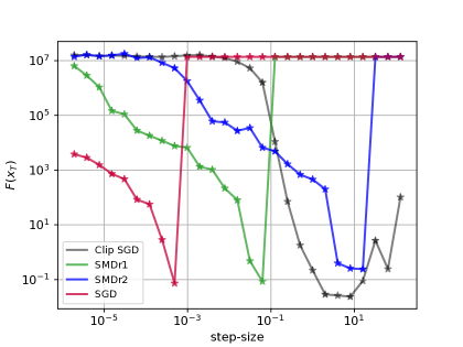
Figure 1: Sensitivity to step-size choice for SMDr1, SMDr2, SGD and Clip SGD (with clipping radius $1$). The plot shows the function value $F(x_{T})$ after $T=10^{4}$ iterations for each step-size. The star markers correspond to the actual runs, and the lines linearly interpolate between them.

To illustrate the empirical performance of the above scheme, we consider two layer autoencoder problem

$$\min {}_{\begin{array}{c}W{}_1\in ℝ{}^{d{}_e\times d{}_f}\\ W{}_2\in ℝ{}^{d{}_f\times d{}_e}\end{array}[F(W):=\frac{1}{n}\sum {}_{i=1}{}^n\parallel W{}_{2}W{}_{1}a{}_i-a{}_i\parallel {}_2{}^2],wherea{}_i\in ℝ{}^{d{}_f}areflattenedrepresentationsofimages,W=[W{}_1,W{}_2]arelearnedparametersofthemodel.TheaboveproblemisnonconvexandgloballynonsmoothinWsinceitsHessiannormgrowsasapolynomialinthenormofW.Therefore,\mathrm{𝖲𝖦𝖣}caneasilydivergeifpoorlyinitialized.However,condition(\text{<a href="\#S5.E8" title="Equation 8 ‣ 5.3 Training Autoencoder Model using SMD ‣ 5 NEW INSIGHTS FOR MACHINE LEARNING" class="ltx\_ref ltx\_font\_italic" style="font-size:70\%;"><span class="ltx\_text ltx\_ref\_tag">8</span></a>})canbeverifiedforsomer{}_0\ge 2andthescheme(\text{<a href="\#S5.E9" title="Equation 9 ‣ 5.3 Training Autoencoder Model using SMD ‣ 5 NEW INSIGHTS FOR MACHINE LEARNING" class="ltx\_ref ltx\_font\_italic" style="font-size:70\%;"><span class="ltx\_text ltx\_ref\_tag">9</span></a>}),(\text{<a href="\#S5.E10" title="Equation 10 ‣ 5.3 Training Autoencoder Model using SMD ‣ 5 NEW INSIGHTS FOR MACHINE LEARNING" class="ltx\_ref ltx\_font\_italic" style="font-size:70\%;"><span class="ltx\_text ltx\_ref\_tag">10</span></a>})provablyconvergesforanyr\ge r{}_0.Wefocusonr=1,2andcallthecorrespondingmethods\mathrm{𝖲𝖬𝖣𝗋𝟣}and\mathrm{𝖲𝖬𝖣𝗋𝟤}.Wecomparethesealgorithmstothestandard\mathrm{𝖲𝖦𝖣},whichcorrespondstor=0.Forcomparison,wealsoincludeapopularheuristicalgorithm,\mathrm{𝖢𝗅𝗂𝗉𝖲𝖦𝖣},whichisknowntomitigatetheproblemofexplodinggradients.Weuseconstantstep-sizesforeachmethod.Figure\text{<a href="\#S5.F1" title="Figure 1 ‣ 5.3 Training Autoencoder Model using SMD ‣ 5 NEW INSIGHTS FOR MACHINE LEARNING" class="ltx\_ref ltx\_font\_italic" style="font-size:70\%;"><span class="ltx\_text ltx\_ref\_tag">1</span></a>}reportsthefinaltraininglossforeachstep-sizeintherange\{2{}^{-19},2{}^{-18},\mathrm{\dots },2{}^7\}.WeobservefromFigure\text{<a href="\#S5.F1" title="Figure 1 ‣ 5.3 Training Autoencoder Model using SMD ‣ 5 NEW INSIGHTS FOR MACHINE LEARNING" class="ltx\_ref ltx\_font\_italic" style="font-size:70\%;"><span class="ltx\_text ltx\_ref\_tag">1</span></a>}that\mathrm{𝖲𝖬𝖣𝗋𝟣}and\mathrm{𝖲𝖬𝖣𝗋𝟤}allowformuchlargerstep-sizesthan\mathrm{𝖲𝖦𝖣}.Moreover,increasingralsoincreasestherobustnesstothestep-sizechoice,i.e.,thelowerpartofthecurvebecomeswider.Atthesametime,inthehighaccuracyregime,\mathrm{𝖢𝗅𝗂𝗉𝖲𝖦𝖣}stilloutperformsotheralgorithmsonthistask.Note,however,that\mathrm{𝖢𝗅𝗂𝗉𝖲𝖦𝖣}mightnotconvergeingeneralinthestochasticsettingforaconstantclippingparameter,see,e.g.,\text{<cite class="ltx\_cite ltx\_citemacro\_citep"><span id="A1.Ex35.m1.1.1.1.1042.1.1nest" class="ltx\_text" style="font-size:70\%;">(</span><span class="ltx\_ref ltx\_missing\_citation ltx\_ref\_self">koloskova2023revisiting</span><span id="A1.Ex35.m1.1.1.1.1042.3.3nest" class="ltx\_text" style="font-size:70\%;">)</span></cite>}.\text{Acknowledgments}ThisworkissupportedbyETHAICenterDoctoralFellowshipandSwissNationalScienceFoundation(SNSF)ProjectFundingNo.200021-207343.\text{References12016Abadietal.Abadi,Chu,Goodfe}}$$