The $\mathsf{SMART}$ Approach to Instance-Optimal Online Learning

Abstract

We devise an online learning algorithm – titled Switching via Monotone Adapted Regret Traces ($\mathsf{SMART}$) – that adapts to the data and achieves regret that is instance optimal, i.e., simultaneously competitive on every input sequence compared to the performance of the follow-the-leader ($\mathsf{FTL}$) policy and the worst case guarantee of any other input policy $\mathsf{ALG}_{\mathsf{WC}}$. We show that the regret of the $\mathsf{SMART}$ policy on any input sequence is within a multiplicative factor $e/(e-1)\approx 1.58$ of the smaller of: 1) the regret obtained by $\mathsf{FTL}$ on the sequence, and 2) the upper bound on regret guaranteed by the given worst-case policy. This implies a strictly stronger guarantee than typical ‘best-of-both-worlds’ bounds as the guarantee holds for every input sequence regardless of how it is generated. $\mathsf{SMART}$ is simple to implement as it begins by playing $\mathsf{FTL}$ and switches at most once during the time horizon to $\mathsf{ALG}_{\mathsf{WC}}$. Our approach and results follow from an operational reduction of instance optimal online learning to competitive anaylsis for the ski-rental problem. We complement our competitive ratio upper bounds with a fundamental lower bound showing that over all input sequences, no algorithm can get better than a $1.43$-fraction of the minimum regret achieved by $\mathsf{FTL}$ and the minimax-optimal policy. We also present a modification of $\mathsf{SMART}$ that combines $\mathsf{FTL}$ with a “small-loss” algorithm to achieve instance optimality between the regret of $\mathsf{FTL}$ and the small loss regret bound.

1 Introduction

Our work aims to develop algorithms for online learning that are instance optimal (Fagin et al., 2001),(Roughgarden, 2021, Chapter $3$) with respect to the stochastic and minimax optimal algorithms for a given setting. This is best motivated via a concrete example:

Example 1 (Binary Prediction).

We are given bit stream $y^{n}\mathrel{\mathop{\mathrel{\mathop{\mathchar 58\relax}}}}=y_{1},y_{2},\ldots,y_{n}\in\{0,1\}^{n}$. At the start of day $t$, before seeing $y_{t}$, we choose (possibly randomized) prediction $\widehat{Y}_{t}\sim\mathrm{Bernoulli}(a_{t})$ (for $a_{t}\in[0,1]$) for the upcoming bit $y_{t}$, given the history $y^{t-1}$. Our resulting loss on day $t$ is $\ell_{t}(a_{t})=\mathbb{P}(\widehat{Y}_{t}\neq y_{t})=|a_{t}-y_{t}|$, and our total loss is $L_{n}(\mathsf{ALG},y^{n})\mathrel{\mathop{\mathrel{\mathop{\mathchar 58\relax}}}}=\sum_{t=1}^{n}\ell_{t}(a_{t})$. The objective is to achieve low regret (i.e., additive loss) compared to the loss $L_{n}(a,y^{n})=\sum_{t=1}^{n}\ell_{t}(a)$ of the best fixed action $a^{*}\in[0,1]$ in hindsight. As $a^{*}$ is the majority in $y^{n}$ between 0 and 1, it follows that $L_{n}(a^{*},y^{n})=\min\left\{\sum_{t=1}^{n}y_{t},n-\sum_{t=1}^{n}y_{t}\right\}$. Formally, for sequence $y^{n}\in\{0,1\}^{n}$, policy $\mathsf{ALG}$ incurs regret

$$\mathrm{Reg}(\mathsf{ALG},y^{n}) \mathrel{\mathop{\mathrel{\mathop{\mathchar 58\relax}}}}=L_{n}(\mathsf{ALG},y^{n})-L_{n}(a^{*},y^{n})=\textstyle\sum_{t=1}^{n}|a_{t}-y_{t}|-\min_{a\in[0,1]}\textstyle\sum_{t=1}^{T}|a-y_{t}|.$$ (1)

Binary prediction goes back to the seminal works of Blackwell (1956) and Hannan (1957). The definition of regret is motivated by the case where $y_{t}$ is randomly generated as i.i.d. Bernoulli$(p)$. If $p$ is known, then the optimal policy is the ‘Bayes predictor’ $a^{\textsf{Bayes}}=\lfloor 2p\rfloor$ (i.e., nearest integer to $p$), which coincides with hindsight optimal $a^{*}$ with high probability when $p$ is away from $1/2$. When $p$ is unknown, the stochastic optimal policy is the Follow The Leader or $\mathsf{FTL}$ policy, which sets $a_{t}=\mathsf{Majority}(y^{t-1})$, i.e. the majority bit amongst the first $t-1$ bits ($a_{t}=1/2$ if both are equal).

A starting point for online learning is the observation that it is easy to construct a sequence $y^{n}$ such that $\mathsf{FTL}$ has poor regret: For example, if $y^{n}=(1,0,1,0,1,0,\ldots)$, i.e., alternate $1$s and $0$s, then the regret of $\mathsf{FTL}$ grows linearly with $n$. In contrast, worst-case optimal online learning policies such as those of Blackwell and Hannan, or more modern versions like Multiplicative Weights or Follow The Perturbed Leader (see Cesa-Bianchi and Lugosi (2006); Slivkins (2019)) guarantee regret of $\Theta(\sqrt{n})$ over all sequences. Indeed, for bit prediction, the exact minimax optimal policy was established by Cover (1966), and this policy (which we refer to as $\mathsf{Cover}$) achieves $\mathrm{Reg}(\mathsf{Cover},y^{n})=\sqrt{\frac{n}{2\pi}}(1+o(1))$ under any $y^{n}\in\{0,1\}^{n}$, implying it is an equalizer (achieves same regret over all sequences).

While the above discussion seems a convincing endorsement of worst-case online learning algorithms, the situation is more complicated. One problem is that while $\mathsf{FTL}$ has bad regret on certain pathological sequences, on more ‘realistic’ sequences $\mathsf{FTL}$ performs orders of magnitude better than the minimax regret. As an example, with i.i.d. Bernoulli$(p)$ input, $\mathrm{Reg}(\mathsf{FTL},y^{n})$ is actually independent of $n$ (i.e., $O(1)$) as long as $p$ is away from $1/2$ with high probability. We demonstrate this in Figure 1$(a)$, where we see $\mathrm{Reg}(\mathsf{FTL})$ is much lower than $\mathrm{Reg}(\mathsf{Cover})\approx 0.39\sqrt{n}$ unless $p$ is very close to $1/2$. This phenomena is known in more general settings (Huang et al., 2016), suggesting that in practice one may be better off just using $\mathsf{FTL}$. On the other hand, as Figure 1$(b,c)$ indicates, we know how to generate sequences $y^{n}$ (Feder et al., 1992) for which $\mathrm{Reg}(\mathsf{FTL},y^{n})$ grows linearly with $n$, and so the $\sqrt{n}$ regret of $\mathsf{Cover}$ becomes appealing.

Now suppose instead that a fictitious oracle is told beforehand which of $\mathsf{FTL}$ or $\mathsf{Cover}$ is better suited for the upcoming sequence $y^{n}$; the demand made by instance optimality is that we try to be competitive against such an oracle on every sequence $y^{n}$.

Definition 1 (Instance Optimality).

A binary prediction policy $\mathsf{ALG}$ is instance optimal with respect to the regret of $\mathsf{FTL}$ and $\mathsf{Cover}$ if there exists some universal $\gamma_{n}\geq 1$ such that for all $y^{n}\in\{0,1\}^{n}$:

$$\small\mathrm{Reg}(\mathsf{ALG},y^{n})\leq\gamma_{n}\min\{\mathrm{Reg}(\mathsf{FTL},y^{n}),\mathrm{Reg}(\mathsf{Cover},y^{n})\}$$

We henceforth refer to $\gamma_{n}$ as the competitive ratio achieved by $\mathsf{ALG}$; ideally we want this ratio to be a constant, i.e., $\gamma_{n}=O(1)$. This necessitates that on sequences where $\mathsf{FTL}$ gets a constant regret, then $\mathsf{ALG}$ basically follows $\mathsf{FTL}$ throughout, while on sequences where $\mathsf{FTL}$ has high (in particular, $\omega(\sqrt{n})$) regret, then $\mathsf{ALG}$ follows $\mathsf{Cover}$ in most rounds.

The challenge in designing instance optimal algorithms is that the regret of any algorithm is a quantity that is not adapted to the natural filtration, i.e. it may not be possible to track $\mathrm{Reg}(\mathsf{ALG},y^{n})$ for any $\mathsf{ALG}$ from just the history $(y_{1},y_{2},\ldots,y_{t-1})$, since the hindsight optimal action $a^{*}$ depends on the entire sequence $y^{n}$. One proxy is to track an algorithm’s loss instead, leading to the idea of ‘corralling’ policies (Agarwal et al., 2017; Pacchiano et al., 2020; Dann et al., 2023), that run online learning over the reference algorithms to get within $O(\text{poly}(n))$ of the smaller of the two losses. Such an approach can not ensure $\gamma_{n}=O(1)$: for example, consider an i.i.d. sequence of Bernoulli$(0.1)$ bits, where $\mathsf{FTL}$ has lower regret than $\mathsf{Cover}$. With high probability on any such sequence we have small $\mathrm{Reg}(\mathsf{FTL},y^{n})=O(1)$ and yet high loss $L_{n}(a^{*},y^{n})=\Theta(n)$; now any corralling algorithm (even a small loss one) must suffer $O(\text{poly}(n))$ regret, and hence $\omega(1)$ competitive ratio. This example also shows that achieving a constant factor guarantee with respect to the minimum of the two losses does not translate to a constant factor guarantee with respect to the minimum of the two regrets.

The instance optimal guarantee is closely related to best-of-both-worlds guarantees, which aim for algorithms that simultaneously achieve (up to constant factors) both the low pseudoregret guarantee of policies designed for stochastic inputs (as with $\mathsf{FTL}$ in our setting, or the Upper Confidence Bound ($\mathsf{UCB}$) algorithm in bandits), as well as a per-sequence regret guarantee comparable to a worst-case optimal algorithm $\mathsf{ALG}_{\mathsf{WC}}$ (Eg. $\mathsf{Cover}$ or Hedge in online learning; $\mathsf{EXP}3$ in bandits Auer et al. (2002a)). Such guarantees have been shown in a variety of settings, including online learning (De Rooij et al., 2014; Orabona and Pál, 2015; Mourtada and Gaïffas, 2019; Bilodeau et al., 2023) and bandit settings (Bubeck and Slivkins, 2012; Zimmert and Seldin, 2019; Lykouris et al., 2018; Dann et al., 2023). One problem though is that since pseudoregret and worst-case regret are very different quantities, the above results tend to be hard to interpret, and less predictive of good performance. Note though that given a pair of stochastic/worst-case optimal algorithms, a policy that is $\gamma$-instance-optimal w.r.t. these immediately satisfies a best-of-both-worlds guarantee with constant factor $\gamma$. In this regard, instance optimality provides a stronger guarantee as it holds on every sequence $y^{n}$ regardless of how it is generated. Moreover, the parameter $\gamma$ can also provide sharper comparisons between algorithms, as well as admit hardness results on the limits of such guarantees.

1.1 Our Contributions

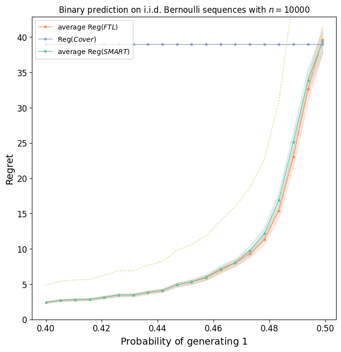
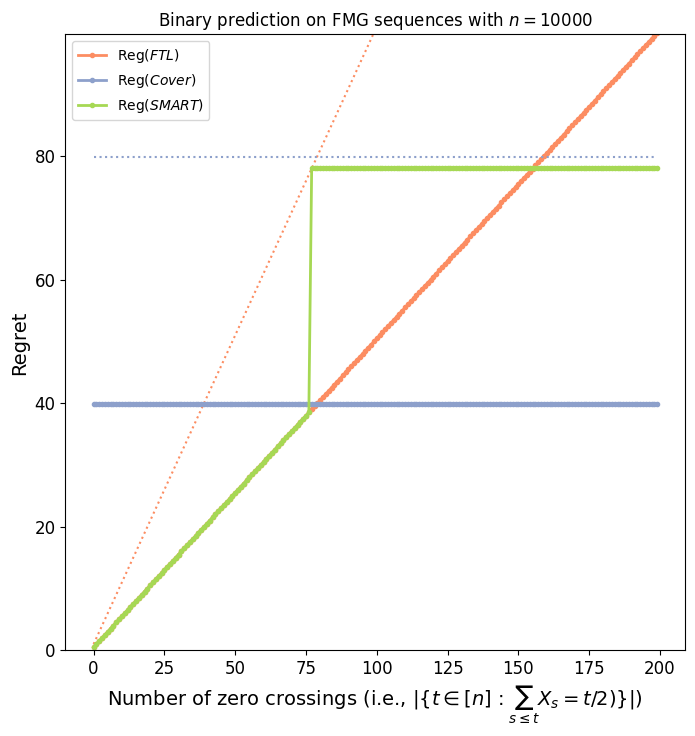
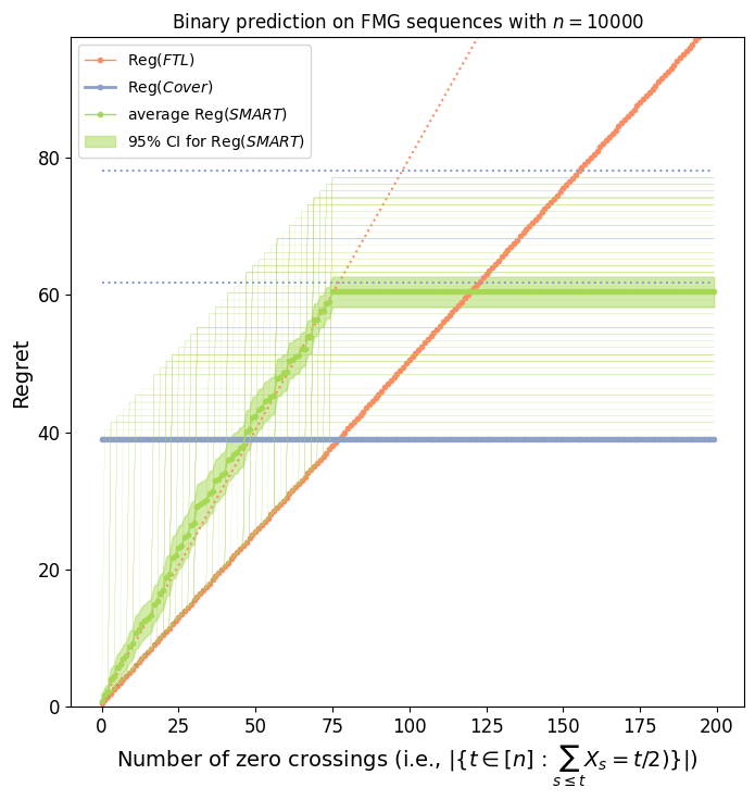
Figure 1: Comparing regret of $\mathsf{FTL}$, $\mathsf{Cover}$ and $\mathsf{SMART}$ on a collection of input sequences (for fixed $n$).
$\bullet$ In Fig. $(a)$, we consider i.i.d. Bernoulli$(p)$ inputs for varying $p$. The regret of $\mathsf{FTL}$ is much lower than $\mathsf{Cover}$ for $p<1/2$; the regret of $\mathsf{SMART}$ tracks $\mathsf{FTL}$ closely (better than $2\mathrm{Reg}(\mathsf{FTL})$, indicated by dotted line).
$\bullet$ In Fig. $(b)$ and $(c)$, we consider ‘worst-case’ binary sequences (as per (Feder et al., 1992)) parameterized by the number of ‘lead-changes’: the sequence with parameter $c$ comprises of $c$ pairs ‘$0,1$’ or ‘$1,0$’, followed by $n-2c$ ‘$1$’s. In Fig. $(b)$, we consider $\mathsf{SMART}$ with a deterministic switching threshold (Theorem 1) and compare $\mathrm{Reg}(\mathsf{SMART})$ with $2\mathrm{Reg}(\mathsf{FTL})$ and $2\mathrm{Reg}(\mathsf{Cover})$ (dotted lines); in Fig. $(c)$, we use a randomized threshold (Theorem 2), and show the average regret over the randomized threshold, as well as sample paths (plotted in green), and compare with $\frac{e}{e-1}$ times $\mathrm{Reg}(\mathsf{FTL})$ and $\mathrm{Reg}(\mathsf{Cover})$ (dotted lines).

We consider a general online learning setting where at the beginning of each round $t\in[n]$, a policy $\mathsf{ALG}$ first plays an action $a_{t}\in\mathcal{A}$, following which, a loss function $\ell_{t}\mathrel{\mathop{\mathchar 58\relax}}\mathcal{A}\to[0,1]$ is revealed, resulting in a loss of $\ell_{t}(a_{t})$. The regret is defined according to:

$$\mathrm{Reg}(\mathsf{ALG},\ell^{n})=\textstyle\sum_{t=1}^{n}\ell_{t}(a_{t})-\inf_{a\in\mathcal{A}}\textstyle\sum_{t=1}^{n}\ell_{t}(a).$$ (2)

More generally, as in with bit prediction, we allow $\mathsf{ALG}$ to play in round $t$ a measure $w_{t}\in\Delta_{\mathcal{A}}$ (i.e., play $\{w_{t}\mathrel{\mathop{\mathchar 58\relax}}\mathcal{A}\mapsto[0,1]|\sum_{a\in\mathcal{A}}w_{t}(a)=1\}$), resulting in an expected loss of $\sum_{a\in\mathcal{A}}w_{t}(a)\ell_{t}(a)$. For notational convenience, we henceforth use $(a_{t},\ell_{t}(a_{t}))$ for the action/loss, and reserve use of expectations for randomness in the algorithm and/or sequence.

We want to understand when is it possible to attain instance optimality as in Eq. (1) with respect to a given pair of algorithms. Ideally, we want the first to be optimal for stochastic instances, and the second to be minimax optimal; unfortunately however exact optimal policies are unknown except in simple settings. To this end, we make two amendments to our goal: First, for the stochastic optimal policy, we use $\mathsf{FTL}$; this is well defined in any online learning setting, and moreover, known to be optimal or near-optimal for a wide range of settings under minimal assumptions (Kotłowski, 2018). Second, instead of the minimax policy, we use as reference any policy $\mathsf{ALG}_{\mathsf{WC}}$ which has a known worst case regret bound $g(n)$. With these modifications in place, we have the following objective.

Definition 2.

Given $\mathsf{FTL}$ and any algorithm $\mathsf{ALG}_{\mathsf{WC}}$ with $\sup_{\ell^{n}}\mathrm{Reg}(\mathsf{ALG}_{\mathsf{WC}},\ell^{n})\leq g(n)$, we say a policy $\mathsf{ALG}$ is instance optimal with respect to the pair if there exists some universal $\gamma_{n}\geq 1$ (i.e. not depending on $y^{n}$) such that for every sequence of losses $\ell^{n}$:

$$\small\mathrm{Reg}(\mathsf{ALG},\ell^{n})\leq\gamma_{n}\min\{\mathrm{Reg}(\mathsf{FTL},\ell^{n}),g(n)\}$$

While the above guarantee is not truly instance-optimal in that we are comparing against a worst-case regret bound $g(n)$ for $\mathsf{ALG}_{\mathsf{WC}}$ rather than its performance on the instance $\ell^{n}$, the two are the same if $\mathsf{ALG}_{\mathsf{WC}}$ is minimax optimal and hence attaining equal regret on all loss sequences; recall this is true of $\mathsf{Cover}$ for binary prediction.

To realize the above goal, we propose the Switch via Monotone Adapted Regret Traces ($\mathsf{SMART}$) approach, which at a high level is a black-box way to convert design of instance-optimal policies into a simple optimal stopping problem. Our approach depends on just two ingredients: first, owing to the additive structure of online learning problems, we have that the minimax guarantee $g(k)$ above holds over any $k\in\mathbb{Z}$ and any (sub)sequence of $n$ loss functions; second, we show that $\mathsf{FTL}$ admits simple anytime regret estimator $\Sigma^{\mathsf{FTL}}_{\tau}$ (see Lemma 1) which is monotone and adapted (i.e., a function only of historical data). Using these two observations, we can reduce the task of minimizing regret to a version of the ‘ski-rental’ problem (Karlin et al., 1994; Borodin and El-Yaniv, 2005), as follows: we play $\mathsf{FTL}$ up to some stopping time $\tau$, and then switch to $\mathsf{ALG}_{\mathsf{WC}}$ for the remaining $n-\tau$ periods, resetting all losses to zero. This algorithm incurs a total regret bounded by $\Sigma^{\mathsf{FTL}}_{\tau}+g(n-\tau)$, and using ideas from competitive analysis, we get that there is a simple way to choose the stopping time $\tau$ to achieve an $e/(e-1)\approx 1.58$-competitive ratio guarantee with respect to the minimum between the regret of $\mathsf{FTL}$ and the worst case guarantee $g(n)$.

Theorem.

(See Theorem 2) Let $\mathsf{ALG}_{\mathsf{WC}}$ have worst-case regret $\sup_{\ell^{n}}\mathrm{Reg}(\mathsf{ALG}_{\mathsf{WC}},\ell^{n})\leq g(n)$ where $g(n)$ is some monotonic function of $n$. An instantiation of $\mathsf{SMART}$ achieves

$$\small\mathrm{Reg}(\mathsf{SMART},\ell^{n})\leq\frac{e}{e-1}\min\{\mathrm{Reg}(\mathsf{FTL},\ell^{n}),g(n)\}+1.$$ (3)

A highlight of our approach is the surprising simplicity of the algorithm and analysis, despite the strength of the instance optimality guarantee. In particular, our approach is modular, allowing one to plug in any $\mathsf{ALG}_{\mathsf{WC}}$ and corresponding worst case bound $g(n)$, thus letting us handle any online learning setting with known minimax bounds. This results in an entire family of instance optimal policies for settings such as predictions with experts and online convex optimization. Moreover, the approach is easy to extend to get more complex guarantees; as an example, if $\mathsf{ALG}_{\mathsf{WC}}$ is designed to get low regret for benign (i.e., ‘small-loss’) sequences $\ell^{n}$, then we show how to use $\mathsf{SMART}$ as a subroutine and achieve an instance optimal guarantee with respect to the regret of $\mathsf{FTL}$ and a small loss regret bound.

Corollary 1 (Following Theorem 5).

Consider the prediction with expert advice setting (Cesa-Bianchi et al., 1997), where $\mathcal{A}=\Delta^{m-1}$, the $m-$simplex for $m\geq 2$, and $\ell_{t}(a)=\langle a,\ell_{t}\rangle$ for $\ell_{t}\in[0,1]^{m}$. Let $L^{*}\mathrel{\mathop{\mathrel{\mathop{\mathchar 58\relax}}}}=\min_{j}\sum_{t=1}^{n}\ell_{tj}$. An instantiation of $\mathsf{SMART}$ achieves

$$\mathrm{Reg}(\mathsf{SMART},\ell^{n}) \leq 2\min\left\{\mathrm{Reg}(\mathsf{FTL},\ell^{n}),10\sqrt{2L^{*}\log m}\right\}+O(\log L^{*}\log m).$$

Finally, studying instance optimality also lets us understand the fundamental limits of best-of-both worlds algorithms. To this end, we provide a lower bound that shows our algorithm is nearly optimal in the competitive ratio. To the best of our knowledge, this is the first hardness result for best-of-both-worlds guarantees in online learning.

Theorem.

(See Theorem 3) In the binary prediction setting, given any online algorithm $\mathsf{ALG}$, there exist sequences $y^{n}\in\{0,1\}^{n}$ such that:

$$\mathrm{Reg}(\mathsf{ALG},y^{n}) \geq 1.43\min\left\{\mathrm{Reg}(\mathsf{FTL},y^{n}),\mathrm{Reg}(\mathsf{Cover},y^{n})\right\}$$

Note again that in binary prediction, $\mathsf{FTL}$ achieves the optimal pseudoregret under i.i.d. inputs, while $\mathsf{Cover}$ is the true minimax policy; thus, this is a fundamental lower bound on best-of-both-worlds guarantee in any online learning setting.

1.2 Related work

There have been many approaches towards combining stochastic and worst-case guarantees. As we discussed before, there is a large literature on best-of-both-worlds algorithms for both full and partial information settings (Wei and Luo, 2018; Bubeck et al., 2019; Zimmert and Seldin, 2019; Dann et al., 2023), and also more complex settings such as metrical task systems (Bhuyan et al., 2023) and control (Sabag et al., 2021; Goel et al., 2023). Another line of work (Rakhlin et al., 2011; Haghtalab et al., 2022; Block et al., 2022; Bhatt et al., 2023) considers smoothed analysis, where the worst-case actions of the adversary are perturbed by nature. A third approach (Bubeck and Slivkins, 2012; Lykouris et al., 2018; Amir et al., 2020; Zimmert and Seldin, 2019) interpolates between the stochastic and adversarial settings by considering most $\ell_{t}$ to be i.i.d., interspersed with a few adversarially chosen instances (corruptions). Finally, another line considers the data-generating distribution to come from a ball of specified radius around i.i.d. distributions (Mourtada and Gaïffas, 2019; Bilodeau et al., 2023). While all these approaches provide useful insights into the gap between average and worst-case guarantees, one can argue they are all imprecisely specified – given an instance $\{\ell_{t}\}_{t\in[n]}$ in hindsight, there is no clear sense as to which model best ‘explains’ the instance.

Our focus on instance optimality instead follows the approach of better understanding and shaping the per-sequence regret landscape. The origins of this approach arguably come from the seminal work of Cover (1966) for binary prediction (we discuss this in more detail in Section 3), with a later focus on better bounds for benign instances in general online learning (Auer et al., 2002b; Cesa-Bianchi et al., 2005; Hazan and Kale, 2010). More recently, a line of work (Koolen et al., 2014; Van Erven et al., 2015; Van Erven and Koolen, 2016; Gaillard et al., 2014) have studied designing policies that can adapt to different types of data sequences and achieve multiple performance guarantees simultaneously. The main idea is to use multiple learning rates that are weighted according to their empirical performance on the data. While the focus is still primarily on classifying instances based on when they are easier/harder to learn, some of the resulting guarantees have an instance-optimality flavor; for example, Van Erven and Koolen (2016) show how to simultaneously match the performance guarantee (in terms of certain variance bounds) attained by different learning rates in Hedge. Such approaches however need to understand their baseline algorithms in great detail, and use them in a ‘white-box’ way to get their guarantees.

In contrast, our approach fundamentally focuses on combining policies in a black-box way to get instance optimal outcomes. As we mention, this is similar in spirit to corralling bandit algorithms Agarwal et al. (2017); Pacchiano et al. (2020); Dann et al. (2023), as well as more recent work on online algorithms with predictions Bamas et al. (2020); Dinitz et al. (2022); Anand et al. (2022); however, as we mention above, these all get guarantees with respect to the loss of the reference algorithms, which is much weaker than our regret guarantees (though they do so in much more complex settings with partial information and/or state). To our knowledge, the only previous result which attains a comparable instance-optimality guarantee to ours is that of De Rooij et al. (2014) for the experts problem, where the authors propose the $\mathsf{FlipFlop}$ policy which interleaves $\mathsf{Hedge}$ (with varying learning rates) and $\mathsf{FTL}$ to obtain a regret guarantee similar to that of Corollary 1. In fact, their guarantee is stronger as $\mathsf{FlipFlop}$ is shown to be 5.64-competitive with respect to $\min\{\mathrm{Reg}(\mathsf{FTL},\ell^{n}),g(L^{*})\}$ where $g(L^{*})\leq\sqrt{L^{*}\log m}$ (De Rooij et al., 2014, Corollary 16). However, while $\mathsf{FlipFlop}$ depends on a clever choice of learning rates in $\mathsf{Hedge}$, $\mathsf{SMART}$ can black-box interleave $\mathsf{FTL}$ with any worst-case/small-loss algorithm without knowing the inner workings of said algorithm, which we see as a significant engineering strength. More importantly, our approach to this problem is distinct as we focus on the fundamental limits (upper and lower bounds) on the competitive ratio that must be incurred when combining $\mathsf{FTL}$ with a worst-case policy; to the best of our knowledge this viewpoint, and the corresponding reduction to an optimal stopping problem, has not been previously explored.

2 Instance Optimal Online Learning: Achievability via $\mathsf{SMART}$

Given the setting and problem statement above, we can now present the $\mathsf{SMART}$ policy. We do this for a general online learning problem, wherein we want to combine $\mathsf{FTL}$ with any given algorithm $\mathsf{ALG}_{\mathsf{WC}}$ with a worst-case regret guarantee $\sup_{\ell^{n}}\mathrm{Reg}(\mathsf{ALG}_{\mathsf{WC}},\ell^{n})\leq g(n)$. Before presenting the policy, we first need the following regret decomposition for $\mathsf{FTL}$.

Lemma 1 (Regret of $\mathsf{FTL}$).

If $L_{t}(\cdot)\mathrel{\mathop{\mathrel{\mathop{\mathchar 58\relax}}}}=\sum_{i=1}^{t}\ell_{t}(\cdot)$, i.e. the cumulative loss function, then

$$\mathrm{Reg}(\mathsf{FTL},\ell^{n})=\textstyle\sum_{t=1}^{n}(L_{t}(a^{*}_{t-1})-L_{t}(a^{*}_{t})).$$

This is reminiscent of the ‘be-the-leader’ lemma (Kalai and Vempala, 2005; Slivkins, 2019), although never stated explicitly as an exact decomposition.

Proof.

Recall we define $a^{\mathsf{FTL}}_{t}=a^{*}_{t-1}$, and hence $\inf_{a\in\mathcal{A}}\sum_{t=1}^{n}\ell_{t}(a)=L_{n}(a^{*}_{n})$. Now we have

$$\mathrm{Reg}(\mathsf{FTL},\ell^{n}) =\textstyle\sum_{t=1}^{n}\ell_{t}(a^{*}_{t-1})-L_{n}(a^{*}_{n})$$

$$=\textstyle\sum_{t=1}^{n}(L_{t}(a^{*}_{t-1})-L_{t-1}(a^{*}_{t-1}))-L_{n}(a^{*}_{n})$$

$$=\textstyle\sum_{t=1}^{n}(L_{t}(a^{*}_{t-1})-L_{t}(a^{*}_{t}))+\textstyle\sum_{t=1}^{n}(L_{t}(a^{*}_{t})-L_{t-1}(a^{*}_{t-1}))-L_{n}(a^{*}_{n})$$

$$\stackrel{{\scriptstyle(a)}}{{=}}\textstyle\sum_{t=1}^{n}(L_{t}(a^{*}_{t-1})-L_{t}(a^{*}_{t}))$$

where $(a)$ follows since $\sum_{t=1}^{n}(L_{t}(a^{*}_{t})-L_{t-1}(a^{*}_{t-1}))=L_{n}(a^{*}_{n})$ by telescoping. ∎

Next, let $\Sigma^{\mathsf{FTL}}_{t}$ denote the anytime regret that $\mathsf{FTL}$ incurs up to round $t$ (i.e., assuming the game ends after round $t$). From Lemma 1 we have

$$\Sigma^{\mathsf{FTL}}_{t}\mathrel{\mathop{\mathrel{\mathop{\mathchar 58\relax}}}}=\mathrm{Reg}(\mathsf{FTL},\ell^{t})=\textstyle\sum_{i=1}^{t}(L_{i}(a^{*}_{i-1})-L_{i}(a^{*}_{i}))$$ (4)

Now we make three critical observations:

• $\Sigma^{\mathsf{FTL}}_{t}$ is adapted: it can be computed at the end of the $t^{th}$ round

• $\Sigma^{\mathsf{FTL}}_{t}$ is monotone non-decreasing in $t$ (since by definition $L_{i}(a^{*}_{i-1})-L_{i}(a^{*}_{i})\geq 0$)

• $\Sigma^{\mathsf{FTL}}_{t}$ is an anytime lower bound for $\mathrm{Reg}(\mathsf{FTL},\ell^{n})$, with $\Sigma^{\mathsf{FTL}}_{n}=\mathrm{Reg}(\mathsf{FTL},\ell^{n})$

For an input threshold $\theta\geq 0$ and an algorithm $\mathsf{ALG}_{\mathsf{WC}}$, we get the following (meta)algorithm.

Input: Policies $\mathsf{FTL},\mathsf{ALG}_{\mathsf{WC}}$, threshold $\theta$

Initialize $\Sigma^{\mathsf{FTL}}_{0}=0$, $t=1$ ;

while $\Sigma^{\mathsf{FTL}}_{t-1}\leq\theta$ do

      Set $a_{t}=a_{t-1}^{*}$;

       // Play $\mathsf{FTL}$

      Observe $\ell_{t}(\cdot)$;

      Update $L_{t}(\cdot)=L_{t-1}(\cdot)+\ell_{t}(\cdot)$ and $\Sigma^{\mathsf{FTL}}_{t}=\Sigma^{\mathsf{FTL}}_{t-1}+(L_{t}(a_{t-1}^{*})-L_{t}(a_{t}^{*}))$ and $t=t+1$;

     

      end while

     Reset losses to $0$ and play $\mathsf{ALG}_{\mathsf{WC}}$ for remaining rounds (See Figure 2(b)) ;

Algorithm 1 Switching via Monotone Adapted Regret Traces ($\mathsf{SMART}$)

We now have the following performance guarantee for Algorithm 1 for $\theta=g(n)$.

Theorem 1 (Regret of $\mathsf{SMART}$ with deterministic threshold).

We are given $\mathsf{FTL}$, and any other policy $\mathsf{ALG}_{\mathsf{WC}}$ with worst-case regret $\sup_{\ell^{n}}\mathrm{Reg}(\mathsf{ALG}_{\mathsf{WC}},\ell^{n})\leq g(n)$ for some monotone function $g$. Then, playing $\mathsf{SMART}$ with threshold $\theta=g(n)$ ensures

$$\mathrm{Reg}(\mathsf{SMART},\ell^{n})\leq 2\min\{\mathrm{Reg}(\mathsf{FTL},\ell^{n}),g(n)\}+1.$$ (5)

As we mention before, the structure of the $\mathsf{SMART}$ algorithm (and the resulting guarantee) parallels the standard 2-competitive guarantee for the ski-rental problem (Karlin et al., 1994). This is a classical optimal stopping problem, where a principal faces an unknown horizon, and in each period must decide whether to rent a pair of skis for the period (for fixed cost $1) or buy the skis for the remaining horizon (for fixed cost $$B$). The aim is to design a policy which is minimax optimal (over the unknown horizon) with regards to the ratio of the cost paid by the principal, and the optimal cost in hindsight. We further expand on this connection in Section 2.1 for the case of binary prediction. However, the connection suggests a natural follow-up question of whether randomized switching can help (as is the case for ski-rental); the following result answers this in the affirmative.

Theorem 2 (Regret of $\mathsf{SMART}$ with Randomized Thresholds).

We are given $\mathsf{FTL}$ and any other policy $\mathsf{ALG}_{\mathsf{WC}}$ with worst-case regret $\sup_{\ell^{n}}\mathrm{Reg}(\mathsf{ALG}_{\mathsf{WC}},\ell^{n})\leq g(n)$ for some monotone function $g$. Moreover, given random sample $U\sim\text{Unif}[0,1]$, suppose we set

$$\theta=g(n)\ln(1+(e-1)U)$$

Then playing the $\mathsf{SMART}$ policy (Algorithm 1) with random threshold $\theta$ ensures

$$\operatorname{\mathbb{E}}_{\theta} \left[\mathrm{Reg}(\mathsf{SMART},\ell^{n})\right]\leq\frac{e}{e-1}\min\{\mathrm{Reg}(\mathsf{FTL},\ell^{n}),g(n)\}+1.$$

While we state the above as a randomized switching policy, this is more for interpretability – it is easier to view our policy as switching between two black-box algorithms rather than playing a convex combination of the two. However, since we define the loss incurred by any $\mathsf{ALG}$ in round $t$ to be the expected loss when $\mathsf{ALG}$ plays a distribution $w_{t}$ over actions $\mathcal{A}$ (see Section 1.1), therefore we can alternately implement the above by mixing between the actions of $\mathsf{FTL}$ and $\mathsf{ALG}_{\mathsf{WC}}$. More specifically, the above policy induces a monotone mixing rule, where over $t$, the weight on the action suggested by $\mathsf{ALG}_{\mathsf{WC}}$ is non-decreasing.

Remark 1 (Optimality over Monotone Mixing Policies).

The competitive ratio of $\frac{e}{e-1}$ is known to be optimal for the ski-rental problem via Yao’s minmax theorem (Borodin and El-Yaniv, 2005). A direct corollary of this is the optimality of $\mathsf{SMART}$ over algorithms that are single switch (i.e., where the weight on $\mathsf{ALG}_{\mathsf{WC}}$ is non-decreasing in $t$). One difference between our setting and ski-rental is that switching back-and-forth between $\mathsf{FTL}$ and $\mathsf{ALG}_{\mathsf{WC}}$ is possible; see for example the $\mathsf{FlipFlop}$ policy of De Rooij et al. (2014). In Section 3 we provide a fundamental lower bound of $1.43$ on the competitive ratio over all algorithms; this suggests that multiple switching can help get a better competitive ratio (since $e/(e-1)\approx 1.58$), but also, that single-switch policies are surprisingly close to optimal.

2.1 Illustrating the Reduction to Ski Rental in Binary Prediction

Before proving Theorems 1 and 2, we first illustrate the basic idea of our approach and reduction for the binary prediction setting. This is aided by the observation that the regret of $\mathsf{FTL}$ in this setting admits a simple geometric interpretation: for any sequence, and any time $t$, we have that $\Sigma^{\mathsf{FTL}}$ is equal to 1/2 times the number of ‘lead changes’ up to time $t$; where a lead change is a time step $i$ where the count of $1$s and $0$s in the (sub)sequence $y^{i-1}$ is equal (see Figure 2(a)).

Corollary 2 ($\mathsf{FTL}$ for binary prediction).

In binary prediction, for any sequence $y\in\{0,1\}^{n}$ and any time $t\leq n$, define the lead-change counter

$$c(y^{t})\mathrel{\mathop{\mathrel{\mathop{\mathchar 58\relax}}}}=|\{0\leq j\leq t~{}s.t.~{}\sum_{i=1}^{j}y_{i}=\sum_{i=1}^{j}(1-y_{i})\}|.$$

Then we have $\Sigma^{\mathsf{FTL}}_{t}=\frac{1}{2}c(y^{t-1})$ and thus $\mathrm{Reg}(\mathsf{FTL},y^{n})=\frac{1}{2}c(y^{n-1})$.

Corollary 2 follows from the regret decomposition in Lemma 1. Furthermore, since the losses of 0s and 1s are equal at a lead change, it also follows that at a lead change $t$, the anytime regret $\Sigma^{\mathsf{FTL}}_{t}$ is also equal to the hindsight regret incurred by $\mathsf{FTL}$ up to time $t$. Since $\Sigma^{\mathsf{FTL}}_{t}$ only increases in value at lead changes, if the $\mathsf{SMART}$ algorithm switches to $\mathsf{ALG}_{\mathsf{WC}}$, it will only happen after a lead change, and thus $\mathsf{SMART}$ behaves as if it had oracle knowledge of the regret of $\mathsf{FTL}$ from just the history up to the current time.

Consider the instantiation of $\mathsf{SMART}$ where $\mathsf{ALG}_{\mathsf{WC}}=\mathsf{Cover}$ and $g(n)=\sqrt{\frac{n}{2\pi}}$. As mentioned in Section 1, a remarkable property of $\mathsf{Cover}$ is that it is the true minimax optimal algorithm, where $\mathrm{Reg}(\mathsf{Cover},y^{n})=\sqrt{\frac{n}{2\pi}}(1+o(1))$ for all sequences $y^{n}$, such that $g(n)$ is nearly equal to $\mathrm{Reg}(\mathsf{Cover},y^{n})$ regardless of the sequence (Cover, 1966).

It follows that $\mathsf{SMART}$ is equivalent to an algorithm which starts with $\mathsf{FTL}$, plays it until the regret of $\mathsf{FTL}$ matches the minimax regret guaranteed by $\mathsf{Cover}$ for the remaining sequence, and then switches to $\mathsf{Cover}$ until the end. Let $t_{\mathrm{sw}}$ denote the last round $\mathsf{SMART}$ plays $\mathsf{FTL}$ before switching to $\mathsf{ALG}_{\mathsf{WC}}$ (with $t_{\mathrm{sw}}=n$ if it never switches). For a single switch algorithm, the sequence which maximizes the regret is one that maximizes the $\mathsf{FTL}$ regret before the switch at $t_{\mathrm{sw}}$, and minimizes the $\mathsf{FTL}$ after the switch, as depicted in Figure 2(a). For such a sequence, $\Sigma^{\mathsf{FTL}}_{t}=t/4$ at lead changes $t$, such that the regret incurred by the algorithm is linear before the switch, matching the linear cost of renting skis in the ski rental problem. Note that $t_{\mathrm{sw}}$ will necessarily be $o(n)$ in such sequences as the time it takes until $\Sigma^{\mathsf{FTL}}_{t}\geq g(n)$ is linear in $g(n)=o(n)$. After the switch, $\mathsf{Cover}$ will incur regret $\sqrt{\frac{n-t_{\mathrm{sw}}}{2\pi}}(1+o(1))=g(n)(1+o(1))$, matching the fixed cost of buying skis at the switching point; Corollary 3 follows as a result of this analysis. Furthermore, in the binary prediction setting, $\mathsf{SMART}$ achieves the stronger notion of instance optimality stated in Definition 1.

Corollary 3.

For all $y^{n}\in\{0,1\}^{n}$, $\mathsf{SMART}$ with $\mathsf{ALG}_{\mathsf{WC}}=\mathsf{Cover}$ and $\theta=\sqrt{\frac{n}{2\pi}}$ satisfies

$$\mathrm{Reg}(\mathsf{SMART},y^{n}) \leq 2\min\{\mathrm{Reg}(\mathsf{FTL},y^{n}),\mathrm{Reg}(\mathsf{Cover},y^{n})\}+1.$$

$\mathsf{SMART}$ with $\mathsf{ALG}_{\mathsf{WC}}=\mathsf{Cover}$ and $\theta=\sqrt{\frac{n}{2\pi}}\ln(1+(e-1)U)$ for $U\sim\text{Uniform}[0,1]$ satisfies

$$\mathrm{Reg}(\mathsf{SMART},y^{n}) \leq 1.58\min\{\mathrm{Reg}(\mathsf{FTL},y^{n}),\mathrm{Reg}(\mathsf{Cover},y^{n})\}+1.$$

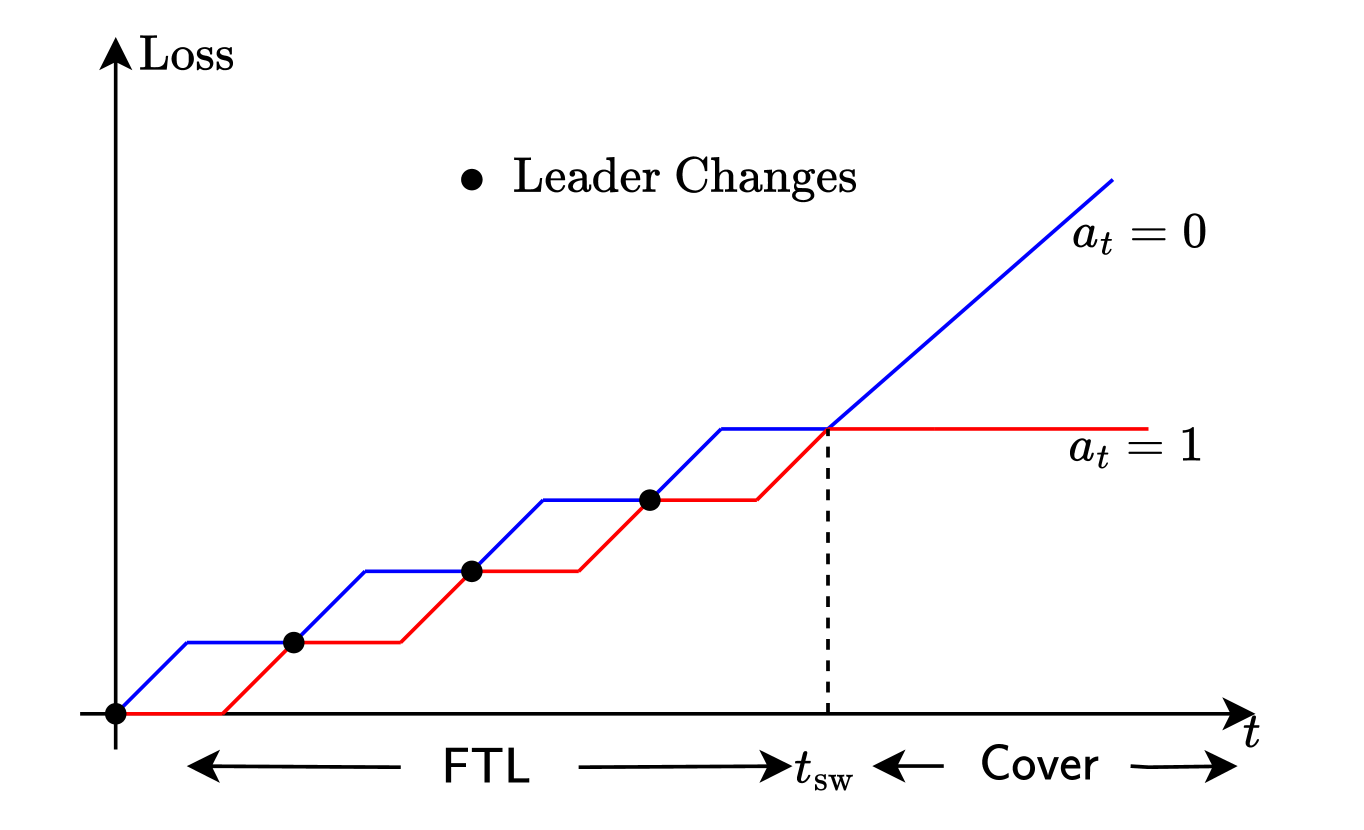
Figure 2: Figure 2(a) on the left shows the worst case instance in binary prediction for an algorithm which starts with $\mathsf{FTL}$ and switches at most once during the time horizon to $\mathsf{Cover}$. Figure2(b) on the right depicts in a prediction with experts setting how $\mathsf{SMART}$ resets the losses after the switch from $\mathsf{FTL}$ to $\mathsf{ALG}_{\mathsf{WC}}$.

2.2 Proofs for General Online Learning

In the general online learning setting, the proof is nearly the same, with the reduction to the ski-rental problem captured by Lemma 2.

Lemma 2.

Let $t_{\mathrm{sw}}\mathrel{\mathop{\mathrel{\mathop{\mathchar 58\relax}}}}=\min_{1\leq t\leq n-1}\Sigma^{\mathsf{FTL}}_{t}>\theta$ denote the last round $\mathsf{SMART}$ plays $\mathsf{FTL}$ before switching to $\mathsf{ALG}_{\mathsf{WC}}$ (with $t_{\mathrm{sw}}=n$ if it never switches). $\mathsf{SMART}$ incurs regret bounded by

$$\mathrm{Reg}(\mathsf{SMART},\ell^{n})\leq\mathrm{Reg}(\mathsf{FTL},\ell^{t_{\mathrm{sw}}})+\mathrm{Reg}(\mathsf{ALG}_{\mathsf{WC}},\ell_{t_{\mathrm{sw}}+1}^{n})\leq\theta+\mathrm{Reg}(\mathsf{ALG}_{\mathsf{WC}},\ell_{t_{\mathrm{sw}}+1}^{n})+1.$$

Proof.

We separately bound the regret of $\mathsf{SMART}$ before the switch and after the switch,

$$\mathrm{Reg}(\mathsf{SMART},\ell^{n}) =\big{(}\textstyle\sum_{t=1}^{t_{\mathrm{sw}}}\ell_{t}(a_{t})-\textstyle\sum_{t=1}^{t_{\mathrm{sw}}}\ell_{t}(a^{*}_{n})\big{)}+\big{(}\textstyle\sum_{t=t_{\mathrm{sw}}+1}^{n}\ell_{t}(a_{t})-\textstyle\sum_{t=t_{\mathrm{sw}}+1}^{n}\ell_{t}(a^{*}_{n})\big{)}$$

$$\stackrel{{\scriptstyle(a)}}{{\leq}}\big{(}\textstyle\sum_{t=1}^{t_{\mathrm{sw}}}\ell_{t}(a_{t})-\textstyle\sum_{t=1}^{t_{\mathrm{sw}}}\ell_{t}(a^{*}_{t_{\mathrm{sw}}})\big{)}+\big{(}\textstyle\sum_{t=t_{\mathrm{sw}}+1}^{n}\ell_{t}(a_{t})-\textstyle\sum_{t=t_{\mathrm{sw}}+1}^{n}\ell_{t}(a^{*}_{t_{\mathrm{sw}}+1\mathrel{\mathop{\mathchar 58\relax}}n})\big{)}$$

$$=\mathrm{Reg}(\mathsf{FTL},\ell^{t_{\mathrm{sw}}})+\mathrm{Reg}(\mathsf{ALG}_{\mathsf{WC}},\ell_{t_{\mathrm{sw}}+1}^{n}).$$

The first term is upper bounded by $\mathrm{Reg}(\mathsf{FTL},\ell^{t_{\mathrm{sw}}})$ since $L_{t_{\mathrm{sw}}}(a^{*}_{n})\geq L_{t_{\mathrm{sw}}}(a^{*}_{t_{\mathrm{sw}}})$ by definition, as $a^{*}_{t_{\mathrm{sw}}}$ is the minimizer of $L_{t_{\mathrm{sw}}}$, and furthermore $\mathsf{SMART}$ always plays according to $\mathsf{FTL}$ in rounds up to $t_{\mathrm{sw}}$. The second term is upper bounded by $\mathrm{Reg}(\mathsf{ALG}_{\mathsf{WC}},\ell_{t_{\mathrm{sw}}+1}^{n})$ because $\sum_{t=t_{\mathrm{sw}}+1}^{n}\ell_{t}(a^{*}_{t_{\mathrm{sw}}+1\mathrel{\mathop{\mathchar 58\relax}}n})\leq\sum_{t=t_{\mathrm{sw}}+1}^{n}\ell_{t}(a^{*}_{n})$ as $a^{*}_{t_{\mathrm{sw}}+1\mathrel{\mathop{\mathchar 58\relax}}n}$ is the minimizer of the losses after $t_{\mathrm{sw}}$, and at time $t>t_{\mathrm{sw}}$, $\mathsf{SMART}$ plays according to $\mathsf{ALG}_{\mathsf{WC}}$ on the sequence of losses limited to $\ell_{t+1}^{n}$. This illustrates the important role of resetting the losses after the switch as depicted in Figure 2(b). Using the fact that $\Sigma^{\mathsf{FTL}}_{t_{\mathrm{sw}}-1}\leq\theta$ and $L_{t_{\mathrm{sw}}-1}(x^{*}_{t_{\mathrm{sw}}-1})\leq L_{t_{\mathrm{sw}}-1}(x^{*}_{t_{\mathrm{sw}}})$, it follows that
$~{}~{}~{}~{}~{}~{}\mathrm{Reg}(\mathsf{FTL},\ell^{t_{\mathrm{sw}}})=\Sigma^{\mathsf{FTL}}_{t_{\mathrm{sw}}-1}+L_{t_{\mathrm{sw}}-1}(a^{*}_{t_{\mathrm{sw}}-1})-L_{t_{\mathrm{sw}}-1}(x^{*}_{t_{\mathrm{sw}}})+\ell_{t_{\mathrm{sw}}}(a^{*}_{t_{\mathrm{sw}}-1})-\ell_{t_{\mathrm{sw}}}(x^{*}_{t_{\mathrm{sw}}})\leq\theta+1.$ ∎

The reduction to ski-rental is again immediate due to the properties that $\Sigma^{\mathsf{FTL}}_{t}\mathrel{\mathop{\mathchar 58\relax}}=\mathrm{Reg}(\mathsf{FTL},\ell^{t_{\mathrm{sw}}})$ is adapted, monotone, and is an anytime lower bound for $\mathrm{Reg}(\mathsf{FTL},\ell^{n})$, while remaining an upper bound on the true regret incurred by $\mathsf{FTL}$ up to time $t$. As a result, the algorithm can pretend that it truly observes the regret it incurs at each time up to the switching time $t_{\mathrm{sw}}$. After the switch, $\mathsf{SMART}$ incurs regret $\mathrm{Reg}(\mathsf{ALG}_{\mathsf{WC}},\ell_{t_{\mathrm{sw}}+1}^{n})$ which is upper bounded by $g(n-t_{\mathrm{sw}})\leq g(n)$ by assumption.

Proof of Theorem 1.

This follows immediately from Lemma 2. For $\ell^{n}$ such that $\mathrm{Reg}(\mathsf{FTL},\ell^{n})\leq g(n)$, $\mathsf{SMART}$ will never switch to $\mathsf{Cover}$ as $\Sigma^{\mathsf{FTL}}_{t}\leq\mathrm{Reg}(\mathsf{FTL},\ell^{n})\leq g(n)$ such that $\mathrm{Reg}(\mathsf{SMART},\ell^{n})=\min\{\mathrm{Reg}(\mathsf{FTL},\ell^{n}),g(n)\}$. For $\ell^{n}$ such that $\mathrm{Reg}(\mathsf{FTL},\ell^{n})>g(n)$, by Lemma 2, $\mathrm{Reg}(\mathsf{SMART},\ell^{n})\leq g(n)+g(n-t_{\mathrm{sw}})+1\leq 2g(n)+1$.
∎

Proof of Theorem 2.

The proof uses a primal-dual approach, similar to that of Karlin et al. (1994) for ski-rental. For a given sequence of loss functions $\ell^{n}$, we use the shorthand $r=\mathrm{Reg}(\mathsf{FTL},\ell^{n})$ and $g=g(n)$. Also, for our given choice of cumulative distribution function $F_{n}$, the corresponding probability density function is given by $f(z)=\frac{e^{z/g}}{g(e-1)}$ for $z\in[0,g]$. As before, let $t_{\mathrm{sw}}\mathrel{\mathop{\mathrel{\mathop{\mathchar 58\relax}}}}=\min_{1\leq t\leq n-1}\Sigma^{\mathsf{FTL}}_{t}>\theta$ be the (random) round where $\mathsf{SMART}$ switches from $\mathsf{FTL}$ to $\mathsf{ALG}_{\mathsf{WC}}$ (with $t_{\mathrm{sw}}=n$ if it never switches). Then by Lemma 2 we have

$$\frac{\mathrm{Reg}(\mathsf{SMART},\ell^{n})-1}{\min\{\mathrm{Reg}(\mathsf{FTL},\ell^{n}),g(n)\}}\leq\begin{cases}\frac{\theta+g}{\min\{r,g\}}&\text{if }t_{\mathrm{sw}}<n\\ 1&\text{if }t_{\mathrm{sw}}=n\end{cases}$$

where the second case follows from the fact that $\theta\in[0,g]$, and hence if we never switch, then $r\leq g(n)$. Taking expectation over $\theta$, we have

$$\frac{\operatorname{\mathbb{E}}_{\theta}\left[\mathrm{Reg}(\mathsf{SMART},\ell^{n})\right]-1}{\min\{\mathrm{Reg}(\mathsf{FTL},\ell^{n}),g\}}\leq\begin{cases}\int_{0}^{r}\frac{x+g}{r}f(x)dx+1-F(r)&\text{if }r\leq g\\ \int_{0}^{g}\frac{x+g}{g}f(x)dx&\text{if }r>g\end{cases}$$

Let $\phi(z)\mathrel{\mathop{\mathrel{\mathop{\mathchar 58\relax}}}}=\int_{0}^{z}\frac{(x+g)}{z}f(x)dx+1-F(z)$ for $z\in[0,g]$; then $\frac{\operatorname{\mathbb{E}}_{\theta}\left[\mathrm{Reg}(\mathsf{SMART},\ell^{n})\right]-1}{\min\{\mathrm{Reg}(\mathsf{FTL},\ell^{n}),g\}}\leq\max_{z\in[0,g]}\phi(z)$. Moreover, we can differentiate to get $z^{2}\phi^{\prime}(z)=gzf(z)-\int_{0}^{z}(x+g)f(x)dx$. Substituting our choice of $f$ in this expression, we get

$$\frac{z^{2}d\phi(z)}{dz} =\frac{ze^{z/g}}{(e-1)}-\int_{0}^{z}(x+g)\frac{e^{x/g}}{g(e-1)}dx=\frac{ze^{z/g}-g\int_{0}^{z/g}(w+1)e^{w}dw}{(e-1)}=0$$

Thus, $\phi(z)$ is constant for all $z\in[0,g]$ and $\phi(g)=\frac{1}{g(e-1)}\int_{0}^{g}(1+x/g)e^{x/g}dx=\frac{e}{e-1}$. ∎

3 Instance Optimal Online Learning: Converse

In this section, we investigate fundamental limits on the instance-optimal regret guarantees achievable by any algorithm. More precisely, in the setting of binary prediction, we ask what is the smallest value of $\gamma_{n}$ satisfying

$$\mathrm{Reg}(\mathsf{ALG},y^{n}) \leq\gamma_{n}\min\{\mathrm{Reg}(\mathsf{FTL},y^{n}),\mathrm{Reg}(\mathsf{Cover},y^{n})\}=\gamma_{n}\min\left\{\tfrac{1}{2}c(y^{n-1}),f_{n}\right\}$$ (6)

for all $y^{n}$, where $f_{n}\mathrel{\mathop{\mathrel{\mathop{\mathchar 58\relax}}}}=\mathrm{Reg}(\mathsf{Cover},y^{n})=\sqrt{\frac{n}{2\pi}}(1+o(1))$. We show the following lower bound.

Theorem 3 (Lower bound on the competitive ratio).

$$\lim_{n\to\infty}\gamma_{n}\geq\Big{(}1-e^{-1/\pi}+2Q\big{(}\sqrt{2/\pi}\big{)}\Big{)}^{-1}\approx 1.4335$$

where the $Q(\cdot)$ function is $Q(x)\mathrel{\mathop{\mathrel{\mathop{\mathchar 58\relax}}}}=\frac{1}{\sqrt{2\pi}}\int_{x}^{\infty}e^{-t^{2}/2}$.

Since binary prediction is a specific online learning problem, this also yields a fundamental lower bound for instance-optimality for general online learning. Note particularly that $\gamma_{n}>1$, implying that $(1+o(1))\min\{\mathrm{Reg}(\mathsf{FTL}),\mathrm{Reg}(\mathsf{ALG}_{\mathsf{WC}})\}$ regret is not possible to achieve. Thus, there is an inevitable multiplicative factor that must be paid in order to achieve an instance-optimal regret guarantee.

An equivalent way to state 6 is to find the smallest $\gamma_{n}$ for which a predictor $\{a_{t}(y^{t-1})\}_{t=1}^{n}$ satisfies for all $y\in\{0,1\}^{n}$

$$\textstyle\sum_{t=1}^{n}|a_{t}(y^{t-1})-y_{t}| \leq\gamma_{n}\min\big{\{}\tfrac{1}{2}c(y^{n-1}),f_{n}\big{\}}+\min\big{\{}\textstyle\sum_{t=1}^{n}y_{i},n-\textstyle\sum_{t=1}^{n}y_{i}\big{\}}.$$ (7)

In order to establish the values of $\gamma_{n}$ for which the loss function in the right hand side of 7 are achievable, we utilize the following result of Cover (1966), which provides an exact characterization of the set of all loss functions achievable in binary prediction. Formally, we say a function $\phi\mathrel{\mathop{\mathchar 58\relax}}\{0,1\}^{n}\to\mathbb{R}^{+}$ is achievable in binary prediction if there exists a predictor/strategy $a_{t}\mathrel{\mathop{\mathchar 58\relax}}y^{t-1}\mapsto[0,1]$ that ensures $\sum_{t=1}^{n}|a_{t}(y^{t-1})-y_{t}|=\phi(y^{n})\quad,\,\forall\,y^{n}\in\{0,1\}^{n}$. Then, we have the following characterization.

Theorem 4 (Cover (1966)).

Let $\epsilon^{n}\sim\mathrm{Bern}\left(\frac{1}{2}\right)$ i.i.d. For $\phi$ to be achievable, it must satisfy the following:

• Balance: $\operatorname{\mathbb{E}}[\phi(\epsilon^{n})]=\frac{n}{2}$ .

• Stability: Let $\phi_{t}(y^{t})\mathrel{\mathop{\mathrel{\mathop{\mathchar 58\relax}}}}=\operatorname{\mathbb{E}}[\phi(y^{t}\epsilon_{t+1}^{n})]$; then $|\phi_{t}(y^{t-1}0)-\phi_{t}(y^{t-1}1)|\leq 1\,\forall t\in[n],\,y^{t}\in\{0,1\}^{t}$.

Further any $\phi$ satisfying the above is realized by predictor $a_{t}(y^{t-1})=\frac{1+\phi_{t}(y^{t-1}0)-\phi_{t}(y^{t-1}1)}{2}$.

As an immediate corollary, Theorem 4 equips us with the exact minimax optimal algorithm for binary prediction alluded to in Section 1. Returning to our setting, from the balance condition in Theorem 4, for $\epsilon^{n}\sim\mathrm{Bern}(1/2)$ i.i.d.

$$\gamma_{n}\operatorname{\mathbb{E}}\big{[}\min\big{\{}\tfrac{1}{2}c(\epsilon^{n-1}),f_{n}\big{\}}\big{]}+\operatorname{\mathbb{E}}\big{[}\min\big{\{}\textstyle\sum_{t=1}^{n}\epsilon_{t},n-\textstyle\sum_{t=1}^{n}\epsilon_{t}\big{\}}\big{]}\geq\frac{n}{2}.$$

for the function in (7) to be achievable. Using the definition of $f_{n}$,

$$\gamma_{n}\geq\frac{f_{n}}{\operatorname{\mathbb{E}}\left[\min\left\{\tfrac{1}{2}c(\epsilon^{n-1}),f_{n}\right\}\right]}=\frac{2f_{n}}{\operatorname{\mathbb{E}}\left[\min\left\{c(\epsilon^{n-1}),2f_{n}\right\}]\right]}.$$

The above bound immediately yields that $\gamma_{n}\geq 1$ as expected. We can further sharply characterize the asymptotics of $\gamma_{n}$, resulting in the stated lower bound. The full proof of Theorem 3 is provided in Appendix B.

4 Instance-Optimal Algorithms in Small-Loss Settings

So far, we have presented specializations of $\mathsf{SMART}$ that achieve instance-optimality between $\mathsf{FTL}$ and the worst-case regret $g(n)$. However, many worst-case algorithms can still adapt to the instance $\ell^{n}$ and achieve regret guarantees that are a function of the ‘difficulty’ of the instance $\ell^{n}$. A common way to quantify this is difficulty is via small-loss bounds, where the regret is upper bounded by $g(L^{*})$ where $g(\cdot)$ as earlier is a monotonic increasing function and $L^{*}\mathrel{\mathop{\mathrel{\mathop{\mathchar 58\relax}}}}=\min_{a\in\mathcal{A}}\sum_{t=1}^{n}\ell_{t}(a)$ is the loss achieved by the best action. Such guarantees imply that for sequences where there exists an action achieving low loss, the corresponding regret achieved is also low. Thus, a natural question is whether $\mathsf{SMART}$ can be specialized to yield an algorithm that is constant competitive with respect to $\min\{\mathrm{Reg}(\mathsf{FTL},\ell^{n}),g(L^{*})\}$.

As a starting point, if $L^{*}$ is known apriori, it is easy to achieve a $\frac{e}{e-1}$ approximation by simply using $\mathsf{SMART}$ with (random) threshold $\theta=g(L^{*})\ln(1+(e-1)U),U\sim\mathrm{Unif}[0,1]$; this is an immediate corollary of Theorem 2. When $L^{*}$ is not known, we use a guess-and-double argument to devise an algorithm that achieves the following instance-optimality guarantee.

Theorem 5 (Regret of $\mathsf{SMART}$ for unknown small loss).

Let $\mathsf{ALG}_{\mathsf{WC}}$ have small loss regret guarantees satisfying $\mathrm{Reg}(\mathsf{ALG}_{\mathsf{WC}},\ell^{n})\leq g(L^{*})$ for any $\ell^{n}$ where $L^{*}=\min_{j\in[m]}L_{tj}$, i.e. the loss achieved by the best expert in hindsight. Then, if we play $\mathsf{SMART}$ for Small-Loss as stated in Algorithm $2$, we have

$$\mathrm{Reg}(\mathsf{SMART},\ell^{n}) \leq 2\min\big{(}\mathrm{Reg}(\mathsf{FTL},\ell^{n}),\textstyle\sum_{z=1}^{\log(1+L^{*}/\log m)+1}g(2^{z}\log m)\big{)}+O(\log L^{*}/\log m)$$

In particular, in the prediction with expert advice setting, we know that $\mathsf{Hedge}$ with a time-varying learning rate achieves $g(L^{*})\equiv 2\sqrt{2L^{*}\log m}+\kappa\log m$ (where $\kappa>0$ is an absolute constant) (Auer et al., 2002b; Cesa-Bianchi et al., 2007); this gives Corollary 1 in Section 1.

The intuitive idea behind the algorithm is to guess the value of $L^{*}$, and play $\mathsf{SMART}$ with this guessed value while simultaneously keeping track of the regret incurred. Whenever the regret incurred exceeds the guarantee established by $\mathsf{SMART}$ with known $L^{*}$ double the guessed value and start again. We use the notation $\mathsf{ALG}_{\mathsf{WC}}(\ell_{t_{1}}^{t_{2}})$ to refer to the worst-case algorithm when the previously observed sequence is $\ell_{t_{1}}^{t_{2}}$; in particular this would be equivalent to the action recommended at time $t_{2}+1$ after throwing away all the observed losses before $t_{1}$. We let $\Sigma^{\mathsf{FTL}}_{t_{1}\mathrel{\mathop{\mathchar 58\relax}}t_{2}}=\sum_{i=t_{1}}^{t_{2}}(L_{i}(a^{*}_{i-1})-L_{i}(a^{*}_{i}))$, which grows as the number of leader changes within $i\in[t_{1},t_{2}]$. The algorithm’s pseudocode is given in Algorithm 2 below, and a proof of Theorem 5 is provided in Appendix A.

Input: Policies $\mathsf{FTL},\mathsf{ALG}_{\mathsf{WC}}$; Small-loss bound $g(\cdot)$

for $z=0,1,\dotsc$ (epochs) do

      Let $t=t_{z}\mathrel{\mathop{\mathrel{\mathop{\mathchar 58\relax}}}}=$start time of $z^{th}$ epoch, $L^{*}_{z}\mathrel{\mathop{\mathrel{\mathop{\mathchar 58\relax}}}}=2^{z}\log m$ (current guess for $L^{*}$), $\Sigma^{\mathsf{FTL}}_{t_{z}\mathrel{\mathop{\mathchar 58\relax}}t_{z}-1}=0$ ;

     

     while $\Sigma^{\mathsf{FTL}}_{t_{z}\mathrel{\mathop{\mathchar 58\relax}}t-1}\leq g(L^{*}_{z})$ do

           Set $a_{t}=a_{t-1}^{*}$;

            // Play $\mathsf{FTL}$

           Observe $\ell_{t}(\cdot)$;

           Update $L_{t}(\cdot)=L_{t-1}(\cdot)+\ell_{t}(\cdot)$ and $\Sigma^{\mathsf{FTL}}_{t_{z}\mathrel{\mathop{\mathchar 58\relax}}t}=\Sigma^{\mathsf{FTL}}_{t_{z}\mathrel{\mathop{\mathchar 58\relax}}t-1}+(L_{t}(a_{t-1}^{*})-L_{t}(a_{t}^{*}))$ and $t=t+1$;

          

           end while

          

          Let $\tau_{z}\mathrel{\mathop{\mathchar 58\relax}}=\min_{t\geq t_{z}}\Sigma^{\mathsf{FTL}}_{t_{z}\mathrel{\mathop{\mathchar 58\relax}}t}>g(L^{*}_{z})$ and $t=\tau_{z}+1$;

           // Check if loss incurred by $\mathsf{ALG}_{\mathsf{WC}}$ in this epoch violates the upper bound from $L_{z}^{*}$ is correct

           while $\sum_{t=t_{z}}^{t}\langle a_{t},\ell_{t}\rangle\leq L_{z}^{*}+2\min\{\Sigma^{\mathsf{FTL}}_{t_{z}\mathrel{\mathop{\mathchar 58\relax}}t},g(L_{z}^{*})\}+1$ do

                Set $a_{t}=\mathsf{ALG}_{\mathsf{WC}}(\ell_{\tau_{z}+1}^{t-1})$ ;

                 // Play $\mathsf{ALG}_{\mathsf{WC}}$ forgetting losses before $\tau_{z}+1$

                Observe $\ell_{t}(\cdot)$;

                Update $L_{t}(\cdot)=L_{t-1}(\cdot)+\ell_{t}(\cdot)$ and $\Sigma^{\mathsf{FTL}}_{t_{z}\mathrel{\mathop{\mathchar 58\relax}}t}=\Sigma^{\mathsf{FTL}}_{t_{z}\mathrel{\mathop{\mathchar 58\relax}}t-1}+(L_{t}(a_{t-1}^{*})-L_{t}(a_{t}^{*}))$ and $t=t+1$;

               

                end while

               

                end for

Algorithm 2 $\mathsf{SMART}$ for Small-Loss

5 Conclusion

In this paper, we present $\mathsf{SMART}$, a simple and black-box online learning algorithm that adapts to the data and achieves instance optimal regret with respect to $\mathsf{FTL}$ and any given worst-case algorithm. We show that $\mathsf{SMART}$ only switches once from $\mathsf{FTL}$ to the worst-case algorithm, and attains a regret that is within a factor of $e/(e-1)\approx 1.58$ of the minimum of the regret of FTL and the minimax regret over all input sequences; we also show that any algorithm must incur an extra factor of at least $1.43$ establishing that our simple approach is surprisingly close to optimal. Furthermore, we extend SMART to incorporate a small-loss algorithm and obtain instance optimality with respect to the small-loss regret bound. Our approach relies on a novel reduction of instance optimal online learning to the ski-rental problem, and leverages tools from information theory and competitive analysis. Our work suggests several open problems for future research, such as finding instance optimal algorithms for bandit settings, or designing algorithms that can adapt to multiple reference algorithms besides FTL and minimax algorithms.

Appendix A Omitted proofs from Section 4

In this Section, we will establish the proofs of Theorem 5 and Corollary 1.

Recall Algorithm 2, where $\mathsf{ALG}_{\mathsf{WC}}(\ell_{t_{1}}^{t_{2}})$ refers to the worst-case algorithm when the previously observed sequence is $\ell_{t_{1}}^{t_{2}}$; in particular this would be equivalent to the action recommended at time $t_{2}+1$ after throwing away all the observed losses before $t_{1}$. We let $\Sigma^{\mathsf{FTL}}_{t_{1}\mathrel{\mathop{\mathchar 58\relax}}t_{2}}=\sum_{i=t_{1}}^{t_{2}}(L_{i}(a^{*}_{i-1})-L_{i}(a^{*}_{i}))$, which grows as the number of leader changes within $i\in[t_{1},t_{2}]$.

We first have the following decomposition of the regret for any algorithm $\mathsf{ALG}$ that plays the sequence of actions $a^{\mathsf{ALG}}_{t}$ at time $t$.

Lemma 3.

The regret incurred by any sequence of actions $(a^{\mathsf{ALG}}_{t})_{t\in[n+1]}$ can be written as

$$\mathrm{Reg}(\mathsf{ALG},\ell^{n}) =\sum_{t=1}^{n}\left(L_{t}(a^{\mathsf{ALG}}_{t})-L_{t}(a^{\mathsf{ALG}}_{t+1})\right),$$ (8)

where we let $a_{n+1}^{\mathsf{ALG}}\mathrel{\mathop{\mathchar 58\relax}}=a_{n}^{*}$.

Proof.

$$L_{n}(\mathsf{ALG}) =\sum_{t=1}^{n}\ell_{t}(a^{\mathsf{ALG}}_{t})$$ (9)

$$=\sum_{t=1}^{n}\left(L_{t}(a^{\mathsf{ALG}}_{t})-L_{t-1}(a^{\mathsf{ALG}}_{t})\right)$$ (10)

$$=L_{n}(a^{\mathsf{ALG}}_{n})+\sum_{t=1}^{n-1}\left(L_{t}(a^{\mathsf{ALG}}_{t})-L_{t}(a^{\mathsf{ALG}}_{t+1})\right)-L_{0}(a^{\mathsf{ALG}}_{1}).$$ (11)

This implies a regret decomposition of

$$\mathrm{Reg}(\mathsf{ALG},\ell^{n}) =L_{n}(\mathsf{ALG})-L_{n}(a_{n}^{*})$$ (12)

$$=L_{n}(a^{\mathsf{ALG}}_{n})-L_{n}(a_{n}^{*})+\sum_{t=1}^{n-1}\left(L_{t}(a^{\mathsf{ALG}}_{t})-L_{t}(a^{\mathsf{ALG}}_{t+1})\right)-L_{0}(a^{\mathsf{ALG}}_{1})$$ (13)

As $L_{0}(a^{\mathsf{ALG}}_{1})=0$, and $a_{n+1}^{\mathsf{ALG}}\mathrel{\mathop{\mathchar 58\relax}}=a_{n}^{*}$, it follows that

$$\mathrm{Reg}(\mathsf{ALG},\ell^{n}) =\sum_{t=1}^{n}\left(L_{t}(a^{\mathsf{ALG}}_{t})-L_{t}(a^{\mathsf{ALG}}_{t+1})\right).$$ (14)

∎

Next, we use this decomposition to establish the regret of any algorithm $\mathsf{ALG}$ that alternates between playing $\mathsf{FTL}$ and another algorithm $\mathsf{ALG}_{\mathsf{WC}}$.

Lemma 4.

Consider an algorithm $\mathsf{ALG}$ which alternates between playing $\mathsf{FTL}$ and $\mathsf{ALG}_{\mathsf{WC}}$, where $\mathsf{FTL}$ is played in the intervals $\{[t_{z},\tau_{z}]\}_{z\in[z_{\mathrm{last}}]}$, and $\mathsf{ALG}_{\mathsf{WC}}$ is played in intervals $\{[\tau_{z}+1,t_{z+1}-1]\}_{z\in[z_{\mathrm{last}}]}$. The regret of $\mathsf{ALG}$ is bounded by

$$\mathrm{Reg}(\mathsf{ALG},\ell^{n})\leq\sum_{z}\left(\Sigma^{\mathsf{FTL}}_{t_{z}\mathrel{\mathop{\mathchar 58\relax}}\tau_{z}-1}+\mathrm{Reg}(\mathsf{ALG}_{\mathsf{WC}},\ell_{\tau_{z}+1}^{t_{z+1}-1})+1\right).$$ (15)

Proof.

We let $t_{z_{\mathrm{last}}}=n+1$, and $a_{n+1}=a_{n}^{*}$. We use Lemma 3 and rearrange the terms by grouping them by the FTL periods and the $\mathsf{ALG}_{\mathsf{WC}}$ periods.

$$\mathrm{Reg} (\mathsf{ALG},\ell^{n})$$

$$=\sum_{z}\left(\sum_{t=t_{z}}^{t_{z+1}-1}(L_{t}(a_{t})-L_{t}(a_{t+1}))\right)$$

$$=\sum_{z}\left(\sum_{t=t_{z}}^{\tau_{z}-1}(L_{t}(a_{t-1}^{*})-L_{t}(a_{t}^{*}))+L_{\tau_{z}}(a_{\tau_{z}-1}^{*})-L_{\tau_{z}}(a_{\tau_{z}+1})+\sum_{t=\tau_{z}+1}^{t_{z+1}-1}(L_{t}(a_{t})-L_{t}(a_{t+1}))\right)$$

$$=\sum_{z}\left(\sum_{t=t_{z}}^{\tau_{z}-1}(L_{t}(a_{t-1}^{*})-L_{t}(a_{t}^{*}))+L_{\tau_{z}}(a_{\tau_{z}-1}^{*})+\sum_{t=\tau_{z}+1}^{t_{z+1}-1}\ell_{t}(a_{t})-L_{t_{z+1}-1}(a_{t_{z+1}})\right)$$

$$=\sum_{z}\sum_{t=t_{z}}^{\tau_{z}-1}(L_{t}(a_{t-1}^{*})-L_{t}(a_{t}^{*}))+\sum_{z}\left(\sum_{t=\tau_{z}+1}^{t_{z+1}-1}\ell_{t}(a_{t})+L_{\tau_{z}}(a_{\tau_{z-1}}^{*})-L_{t_{z+1}-1}(a_{t_{z+1}-1}^{*})\right).$$

We bound the first term by the FTL regret. Recall the notation

$$\Sigma^{\mathsf{FTL}}_{t_{z}\mathrel{\mathop{\mathchar 58\relax}}\tau_{z}-1}\mathrel{\mathop{\mathchar 58\relax}}=\sum_{t=t_{z}}^{\tau_{z}-1}(L_{t}(a_{t-1}^{*})-L_{t}(a_{t}^{*})).$$ (16)

Because we are playing FTL at both time $\tau_{z}$ and $\tau_{z}-1$, it holds that

$$L_{\tau_{z}}(a_{\tau_{z}-1}^{*})=L_{\tau_{z}-1}(a_{\tau_{z}-1}^{*})+\ell_{\tau_{z}}(a_{\tau_{z}-1}^{*})\leq L_{\tau_{z}}(a_{\tau_{z}}^{*})+1.$$

To bound the second term, we will show that

$$\sum_{t=\tau_{z}+1}^{t_{z+1}-1} \ell_{t}(a_{t})+L_{\tau_{z}}(a_{\tau_{z-1}}^{*})-L_{t_{z+1}-1}(a_{t_{z+1}-1}^{*})$$

$$\leq\sum_{t=\tau_{z}+1}^{t_{z+1}-1}\ell_{t}(a_{t})+L_{\tau_{z}}(a_{\tau_{z}}^{*})-L_{t_{z+1}-1}(a_{t_{z+1}-1}^{*})+1$$ (17)

$$=\sum_{t=\tau_{z}+1}^{t_{z+1}-1}\ell_{t}(a_{t})+\min_{a}L_{\tau_{z}}(a)-\min_{a}L_{t_{z+1}-1}(a)+1$$ (18)

$$\leq\sum_{t=\tau_{z}+1}^{t_{z+1}-1}\ell_{t}(a_{t})-\min_{a}\left(L_{t_{z+1}-1}(a)-L_{\tau_{z}}(a)\right)+1$$ (19)

$$=\mathrm{Reg}(\mathsf{ALG}_{\mathsf{WC}},\ell_{\tau_{z}+1}^{t_{z+1}-1})+1.$$ (20)

∎

We now complete the proof of Theorem 3 by showing that the conditions that determine the switching time between $\mathsf{FTL}$ and $\mathsf{ALG}_{\mathsf{WC}}$ are appropriately chosen to upper bound $\Sigma^{\mathsf{FTL}}_{t_{z}\mathrel{\mathop{\mathchar 58\relax}}\tau_{z}-1}$ and $\mathrm{Reg}(\mathsf{ALG}_{\mathsf{WC}},\ell_{\tau_{z}+1}^{t_{z+1}-1})$. Firstly, note that for any $z<z_{\mathrm{last}}$, $\mathrm{Reg}(\mathsf{ALG}_{\mathsf{WC}},\ell_{\tau_{z}+1}^{t_{z+1}-1})>g(L_{z}^{*})$, which implies that $L^{*}>L_{z}^{*}$. In particular, the epoch $z_{\mathrm{last}}-1$ was exited, which implies that

$$2^{z_{\mathrm{last}}-1}\log m\leq L^{*}\implies z_{\mathrm{last}}\leq\log\left(\frac{L^{*}}{\log m}\right)+1$$

By the stopping condition of the epoch, $\mathrm{Reg}(\mathsf{ALG}_{\mathsf{WC}},\ell_{\tau_{z}+1}^{t_{z+1}-1})\leq\mathrm{Reg}(\mathsf{ALG}_{\mathsf{WC}},\ell_{\tau_{z}+1}^{t_{z+1}-2})+1\leq g(L_{z}^{*})+1$, such that substituting into Lemma 4 implies

$$\mathrm{Reg}(\mathsf{SMART},\ell^{n})\leq\sum_{z}\left(\Sigma^{\mathsf{FTL}}_{t_{z}\mathrel{\mathop{\mathchar 58\relax}}\tau_{z}-1}+g(L_{z}^{*})+2\right).$$ (21)

Also, it always holds that $\Sigma^{\mathsf{FTL}}_{t_{z}\mathrel{\mathop{\mathchar 58\relax}}\tau_{z}-1}\leq g(L_{z}^{*})$ and for $z<z_{\mathrm{last}}$, $\Sigma^{\mathsf{FTL}}_{t_{z}\mathrel{\mathop{\mathchar 58\relax}}\tau_{z}}>g(L_{z}^{*})$. Therefore

$$\sum_{z}^{z_{\mathrm{last}}-1}g(L_{z}^{*})<\sum_{z}\Sigma^{\mathsf{FTL}}_{t_{z}\mathrel{\mathop{\mathchar 58\relax}}\tau_{z}-1}\leq\mathrm{Reg}(\mathsf{FTL},\ell^{n})$$

and $\sum_{z}\Sigma^{\mathsf{FTL}}_{t_{z}\mathrel{\mathop{\mathchar 58\relax}}\tau_{z}-1}\leq\sum_{z}^{z_{\mathrm{last}}}g(L_{z}^{*})$.

To put it all together, if $\sum_{z}^{z_{\mathrm{last}}}g(L_{z}^{*})\leq\mathrm{Reg}(\mathsf{FTL},\ell^{n})$, then

$$\mathrm{Reg}(\mathsf{SMART},\ell^{n})\leq 2\sum_{z}g(L_{z}^{*})+2z_{\mathrm{last}}.$$ (22)

If $\mathrm{Reg}(\mathsf{FTL},\ell^{n})<\sum_{z}^{z_{\mathrm{last}}}g(L_{z}^{*})$, then it must be that in the last epoch the algorithm never switches to $\mathsf{ALG}_{\mathsf{WC}}$. If it switched to $\mathsf{ALG}_{\mathsf{WC}}$ it would imply that $\mathrm{Reg}(\mathsf{FTL},\ell^{n})\geq\sum_{z}\Sigma^{\mathsf{FTL}}_{t_{z}\mathrel{\mathop{\mathchar 58\relax}}\tau_{z}}>\sum_{z}^{z_{\mathrm{last}}}g(L_{z}^{*})$ which would violate the assumption that $\mathrm{Reg}(\mathsf{FTL},\ell^{n})<\sum_{z}^{z_{\mathrm{last}}}g(L_{z}^{*})$. Therefore it must be that

$$\mathrm{Reg}(\mathsf{SMART},\ell^{n})\leq 2\mathrm{Reg}(\mathsf{FTL},\ell^{n})+2z_{\mathrm{last}}.$$ (23)

As a result, it follows that (putting the $L^{*}\leq\log m$ and the $L^{*}>\log m$ cases together)

$$\mathrm{Reg} (\mathsf{SMART},\ell^{n})$$

$$\leq 2\min\left(\mathrm{Reg}(\mathsf{FTL},\ell^{n}),\sum_{z=0}^{\log\left(1+\frac{L^{*}}{\log m}\right)+1}g(2^{z}\log m)\right)+2\log\left(1+\frac{L^{*}}{\log m}\right)+2.$$ (24)

A.1 Proof of Corollary 1

This follows from Theorem 5 and by calculating

$$\sum_{z=0}^{\log\left(1+\frac{L^{*}}{\log m}\right)+1} g(2^{z}\log m)$$

$$=2\sqrt{2}\log m\sum_{z=0}^{\log\left(1+\frac{L^{*}}{\log m}\right)+1}2^{z/2}+\kappa\log m\log\left(1+\frac{L^{*}}{\log m}\right)+\kappa\log m$$

$$\leq\log m\frac{4\sqrt{2}}{\sqrt{2}-1}\sqrt{1+\frac{L^{*}}{\log m}}+\kappa\log m\log\left(1+\frac{L^{*}}{\log m}\right)+\kappa\log m$$

$$\leq 10\sqrt{2\log^{2}m+2L^{*}\log m}+\kappa\log m\log\left(1+\frac{L^{*}}{\log m}\right)+\kappa\log m$$

$$\stackrel{{\scriptstyle\text{(a)}}}{{\leq}}10\sqrt{2L^{*}\log m}+\kappa\log\left(1+\frac{L^{*}}{\log m}\right)\log m+10\sqrt{2}\log m+\kappa\log m$$

where (a) follows since for nonnegative $a,b$ $\sqrt{a+b}\leq\sqrt{a}+\sqrt{b}$.

Appendix B Proof of Theorem 3

Consider a large even $n$. We then have for horizon size $n+1$, $\mathrm{Reg}(\mathsf{FTL},y^{n+1})=\frac{c(y^{n})}{2}$. Moreover, $\mathrm{Reg}(\mathsf{Cover},y^{n+1})=f_{n+1}$. Let

$$p_{n,k}\mathrel{\mathop{\mathrel{\mathop{\mathchar 58\relax}}}}=\mathbb{P}[c(\epsilon^{n})=k+1].$$ (25)

We then have,

$$\operatorname{\mathbb{E}}[\min\{c(\epsilon^{n}),2f_{n+1}\}] =\sum_{k=1}^{n}\min\{k,2f_{n+1}\}\Pr[c(\epsilon^{n})=k]$$

$$=\sum_{k=1}^{n}\min\{k,2f_{n+1}\}p_{n,k-1}$$

$$=\sum_{k=0}^{n}\min\{k+1,2f_{n+1}\}p_{n,k}$$

$$=\sum_{k=0}^{\lfloor 2f_{n+1}\rfloor-1}(k+1)p_{n,k}+2f_{n+1}\mathbb{P}[c(\epsilon^{n})\geq 2f_{n+1}]$$

$$=\sum_{k=0}^{\lfloor 2f_{n+1}\rfloor-1}(k+1)p_{n,k}+2f_{n+1}\mathbb{P}[c(\epsilon^{n})\geq 2f_{n+1}]+\mathbb{P}[c(\epsilon^{n})\leq\lfloor 2f_{n+1}\rfloor]$$

$$=\sum_{k=0}^{\lfloor 2f_{n+1}\rfloor-1}kp_{n,k}+2f_{n+1}\left(1-\sum_{k=0}^{\lfloor 2f_{n+1}\rfloor-1}p_{n,k}\right)+\mathbb{P}[c(\epsilon^{n})\leq\lfloor 2f_{n+1}\rfloor]$$ (26)

Upon dividing 26 by $2f_{n+1}$, we get

$$\frac{\operatorname{\mathbb{E}}[\min\{c(\epsilon^{n}),2f_{n+1}\}]}{2f_{n+1}}=\frac{\sum_{k=0}^{\lfloor 2f_{n+1}\rfloor-1}kp_{n,k}}{2f_{n+1}}+\left(1-\sum_{k=0}^{\lfloor 2f_{n+1}\rfloor-1}p_{n,k}\right)+\frac{\mathbb{P}[c(\epsilon^{n})\leq\lfloor 2f_{n+1}\rfloor]}{2f_{n+1}}.$$ (27)

Note that the third term vanishes since $f_{n+1}\to\infty$ and $0\leq\mathbb{P}[\cdot]\leq 1$. We will now separately evaluate the first two terms in 27. To do this, we require an auxiliary lemma, the proof of which is provided later.

Lemma 5.

If $k\leq C\sqrt{n}$ for an absolute constant $C$, then for large enough $n$ ($n\geq 32C^{2}$ suffices) we have

$$e^{-\frac{16C^{3}}{\sqrt{n}}}\leq\frac{p_{n,k}}{\sqrt{\frac{2}{n\pi}}e^{-k^{2}/2n}}\leq\sqrt{\frac{1-C/\sqrt{n}}{1-2C/\sqrt{n}}}e^{\frac{16C^{3}}{\sqrt{n}}}.$$ (28)

That is,

$$p_{n,k}=\sqrt{\frac{2}{n\pi}}e^{-k^{2}/2n}(1+o(1)).$$

We now evaluate the first term in 27. Since $\lfloor 2f_{n+1}\rfloor-1\leq 2\sqrt{n}$, we invoke Lemma 5 to evaluate

$$\sum_{k=0}^{\lfloor 2f_{n+1}\rfloor-1}kp_{n,k} =(1+o(1))\sum_{k=0}^{\lfloor 2f_{n+1}\rfloor-1}k\sqrt{\frac{2}{n\pi}}e^{-\frac{k^{2}}{2n}}$$ (29)

$$=(1+o(1))\sqrt{\frac{2}{n\pi}}\sum_{k=0}^{\lfloor 2f_{n+1}\rfloor-1}ke^{-\frac{k^{2}}{2n}}$$ (30)

Now, we note that since $x\mapsto xe^{-\frac{x^{2}}{2n}}$ is increasing on $(0,\lfloor 2f_{n+1}\rfloor-1)$ , by a Riemann approximation, we have that

$$\int_{0}^{2f_{n+1}-2}xe^{-\frac{x^{2}}{2n}}dx-1\leq\sum_{k=0}^{\lfloor 2f_{n+1}\rfloor-1}ke^{-\frac{k^{2}}{2n}}\leq\int_{0}^{2f_{n+1}}xe^{-\frac{x^{2}}{2n}}dx$$ (31)

and evaluating

$$\int_{0}^{2f_{n+1}}xe^{-\frac{x^{2}}{2n}}dx =\frac{1}{2}\int_{0}^{4f_{n+1}^{2}}e^{-\frac{t}{2n}}dt$$

$$=n\left(1-e^{-\frac{4f_{n+1}^{2}}{2n}}\right)$$

$$=n\left(1-e^{-\frac{1}{\pi}(1+o(1))}\right).$$ (32)

Evaluating the lower bound in 31 analogously we have

$$\sum_{k=0}^{\lfloor 2f_{n+1}\rfloor-1}ke^{-\frac{k^{2}}{2n}}=(1+o(1))n\left(1-e^{-\frac{1}{\pi}(1+o(1))}\right)$$ (33)

and therefore from 30,

$$\frac{\sum_{k=0}^{\lfloor 2f_{n+1}\rfloor-1}kp_{n,k}}{2f_{n+1}} =(1+o(1))\frac{\left(1-e^{-\frac{1}{\pi}(1+o(1))}\right)n\sqrt{\frac{2}{n\pi}}}{\sqrt{\frac{2(n+1)}{\pi}}}$$

$$=(1+o(1))\left(1-e^{-\frac{1}{\pi}(1+o(1))}\right)$$ (34)

and therefore, from 34, we have that

$$\lim_{n\to\infty}\frac{\sum_{k=0}^{\lfloor 2f_{n+1}\rfloor-1}kp_{n,k}}{2f_{n+1}}=1-e^{-\frac{1}{\pi}}.$$ (35)

We now address the second term in 27 by invoking Lemma 5 and noting that

$$\sum_{k=0}^{\lfloor 2f_{n+1}\rfloor-1}p_{n,k} =(1+o(1))\sqrt{\frac{2}{n\pi}}\sum_{k=0}^{\lfloor 2f_{n+1}\rfloor-1}e^{-\frac{k^{2}}{2n}}$$

$$\stackrel{{\scriptstyle(a)}}{{=}}(1+o(1))\int_{0}^{2f_{n+1}}e^{-\frac{x^{2}}{2n}}dx$$

$$=(1+o(1))\sqrt{\frac{2}{\pi}}\int_{0}^{\sqrt{\frac{2}{\pi}}}e^{-\frac{t^{2}}{2}}dt$$

$$=\frac{1}{\sqrt{2\pi}}\int_{-\sqrt{\frac{2}{\pi}}}^{\sqrt{\frac{2}{\pi}}}e^{-\frac{t^{2}}{2}}dt$$

$$=\mathbb{P}\left(-\sqrt{\frac{2}{\pi}}\leq X\leq\sqrt{\frac{2}{\pi}}\right)$$ (36)

where in 36 $X\sim\mathcal{N}(0,1)$. Then,

$$1-\sum_{k=0}^{\lfloor 2f_{n+1}\rfloor-1}p_{n,k} \to 1-\mathbb{P}\left(-\sqrt{\frac{2}{\pi}}\leq X\leq\sqrt{\frac{2}{\pi}}\right)$$

$$=2Q\left(\sqrt{\frac{2}{\pi}}\right).$$ (37)

Substituting 35 and 37 in 27 yields that

$$\frac{1}{\gamma_{n}}=\frac{\operatorname{\mathbb{E}}[\min\{c(\epsilon^{n}),2f_{n+1}\}]}{2f_{n+1}}\to 1-e^{-\frac{1}{\pi}}+2Q\left(\sqrt{\frac{2}{\pi}}\right)$$ (38)

and therefore

$$\gamma_{n}\to\frac{1}{1-e^{-\frac{1}{\pi}}+2Q\left(\sqrt{\frac{2}{\pi}}\right)}.$$ (39)

B.1 Proof of Lemma 5

We first note the following.

Proposition 1 (Feller , Chapter 3, Exercise 11).

$$p_{n,k}=\frac{1}{2^{n-k}}\binom{n-k}{n/2}.$$

Therefore,

$$\frac{p_{n,k}2^{n}}{2^{k}}=\binom{n-k}{n/2}=\frac{(n-k)!}{\frac{n}{2}!\left(\frac{n}{2}-k\right)!}.$$

We now use the Stirling approximation:

$$\sqrt{2\pi m}\left(\frac{m}{e}\right)^{m}e^{\frac{1}{12m+1}}\leq m!\leq\sqrt{2\pi m}\left(\frac{m}{e}\right)^{m}e^{\frac{1}{12m}}.$$ (40)

Using 40 we have

$$\frac{p_{n,k}2^{n}}{2^{k}} \leq\frac{\sqrt{2\pi(n-k)}}{\sqrt{2\pi(n/2)}\sqrt{2\pi(n/2-k)}}\cdot\frac{(n-k)^{n-k}}{(n/2)^{n/2}(n/2-k)^{n/2-k}}$$

$$\qquad\qquad\qquad\qquad\qquad\qquad\cdot\exp{\left(\frac{1}{12(n-k)}-\frac{1}{6n+1}-\frac{1}{6n-12k+1}\right)}$$

$$=\sqrt{\frac{2}{n\pi}}\sqrt{\frac{n-k}{n-2k}}\frac{(n-k)^{n-k}2^{n-k}}{n^{n/2}(n-2k)^{n/2-k}}\cdot\exp{\left(\frac{1}{12n-k}\right)}$$

$$\stackrel{{\scriptstyle(a)}}{{\leq}}\sqrt{\frac{2}{n\pi}}\cdot 2^{n-k}\cdot\frac{(n-k)^{n-k}}{n^{n/2}(n-2k)^{n/2-k}}\exp\left(\frac{1}{12n-k}\right)\cdot\sqrt{\frac{1-C/\sqrt{n}}{1-2C/\sqrt{n}}}$$

$$=\sqrt{\frac{2}{n\pi}}\cdot 2^{n-k}\underbrace{\frac{(1-k/n)^{n-k}}{(1-2k/n)^{n/2-k}}}_{=\mathrel{\mathop{\mathchar 58\relax}}T}\exp\left(\frac{1}{12n-k}\right)\cdot\sqrt{\frac{1-C/\sqrt{n}}{1-2C/\sqrt{n}}}.$$ (41)

We now analyze the term $T$ in 41 in more detail.

Proposition 2.

$$-\frac{k^{2}}{2n^{2}}-c\frac{k^{3}}{n^{2}}\leq\ln T\leq-\frac{k^{2}}{2n^{2}}+c\frac{k^{3}}{n^{2}}$$ (42)

where $c\leq 15$.

Proof.

By Taylor theorem, we have

$$\ln(1-x)=-x-\frac{x^{2}}{2}-\frac{x^{3}}{3(1-\mu)^{2}}\text{ for }\mu\in(0,x).$$ (43)

Therefore, for $k\leq C\sqrt{n}$ and $n\geq 16C^{2}$ we have

$$\ln\left(1-\frac{k}{n}\right) =-\frac{k}{n}-\frac{k^{2}}{2n^{2}}-\frac{\alpha_{1}k^{3}}{n^{3}}$$ (44)

$$\ln\left(1-\frac{2k}{n}\right) =-\frac{2k}{n}-\frac{2k^{2}}{2n^{2}}-\frac{\alpha_{2}k^{3}}{n^{3}}$$ (45)

for $\alpha_{1},\alpha_{2}\in\Big{(}\frac{1}{3},\frac{8}{3}\Big{]}$. Evaluating $\ln T$ we have

$$\ln T =(n-k)\ln\left(1-\frac{k}{n}\right)-\left(n-\frac{k}{2}\right)\ln\left(1-\frac{2k}{n}\right)$$

$$\stackrel{{\scriptstyle(a)}}{{=}}(n-k)\left(-\frac{k}{n}-\frac{k^{2}}{2n^{2}}-\frac{\alpha_{1}k^{3}}{n^{3}}\right)-\left(n-\frac{k}{2}\right)\left(-\frac{2k}{n}-\frac{2k^{2}}{2n^{2}}-\frac{\alpha_{2}k^{3}}{n^{3}}\right)$$

$$=\left(-\frac{k^{2}}{2n}+\frac{k^{2}}{n}+\frac{k^{2}}{n}-\frac{2k^{2}}{n}\right)+\left(-\alpha_{1}+\frac{1}{2}+\frac{\alpha_{2}}{2}-2\right)\frac{k^{3}}{n^{2}}+\left(\alpha_{1}-\alpha_{2}\right)\frac{k^{4}}{n^{3}}$$

$$=-\frac{k^{2}}{2n^{2}}+c_{1}\frac{k^{3}}{n^{2}}+c_{2}\frac{k^{4}}{n^{3}}$$ (46)

where $(a)$ follows by substituting 44 and 45. Now, since $\frac{k^{4}}{n^{3}}\leq\frac{k^{3}}{n^{2}}$ we have

$$\ln T\leq-\frac{k^{2}}{2n^{2}}+(|c_{1}|+|c_{2}|)\frac{k^{3}}{n^{2}}$$ (47)

and on the other hand for the same reason

$$\ln T\geq-\frac{k^{2}}{2n}-(|c_{1}|+|c_{2}|)\frac{k^{3}}{n^{2}}$$ (48)

The proposition follows by noticing $|c_{1}|+|c_{2}|\leq 15$ by using that $\alpha_{1},\alpha_{2}\in\left(\frac{1}{3},\frac{8}{3}\right]$. ∎

Using Proposition 2 in 41 we have the upper bound

$$p_{n,k} \leq\sqrt{\frac{2}{n\pi}}\cdot\exp\left(-\frac{k^{2}}{2n}+\frac{15k^{3}}{n^{2}}\right)\cdot\exp\left(\frac{1}{12n-k}\right)\cdot\sqrt{\frac{1-C/\sqrt{n}}{1-2C/\sqrt{n}}}$$

$$\stackrel{{\scriptstyle(a)}}{{\leq}}\sqrt{\frac{2}{n\pi}}\cdot\exp\left(-\frac{k^{2}}{2n}\right)\cdot\exp\left(\frac{16k^{3}}{n^{2}}\right)\cdot\sqrt{\frac{1-C/\sqrt{n}}{1-2C/\sqrt{n}}}$$

$$\stackrel{{\scriptstyle(b)}}{{\leq}}\sqrt{\frac{2}{n\pi}}\cdot\exp\left(-\frac{k^{2}}{2n}\right)\cdot\exp\left(\frac{16C^{3}}{\sqrt{n}}\right)\cdot\sqrt{\frac{1-C/\sqrt{n}}{1-2C/\sqrt{n}}}$$ (49)

where $(a)$ uses $\frac{1}{12n-k}+\frac{15k^{3}}{n^{2}}\leq\frac{16k^{3}}{n^{2}}$, and $(b)$ uses the fact that $k\leq C\sqrt{n}$, which yields the upper bound in 28. The lower bound follows analogously by the Stirling approximation 40 and Proposition 2.

References

Fagin et al. [2001]
Ronald Fagin, Amnon Lotem, and Moni Naor.
Optimal aggregation algorithms for middleware.
In Proceedings of the twentieth ACM SIGMOD-SIGACT-SIGART symposium on Principles of database systems, pages 102–113, 2001.
Roughgarden [2021]
Tim Roughgarden.
Beyond the worst-case analysis of algorithms.
Cambridge University Press, 2021.
Blackwell [1956]
D Blackwell.
An analog of the minimax theorem for vector payoffs.
Pacific Journal of Mathematics, 6(1):1–8, 1956.
Hannan [1957]
James Hannan.
Approximation to bayes risk in repeated play.
Contributions to the Theory of Games, 3:97–139, 1957.
Cesa-Bianchi and Lugosi [2006]
Nicolo Cesa-Bianchi and Gábor Lugosi.
Prediction, learning, and games.
Cambridge university press, 2006.
Slivkins [2019]
Aleksandrs Slivkins.
Introduction to multi-armed bandits.
Foundations and Trends® in Machine Learning, 12(1-2):1–286, 2019.
Cover [1966]
Thomas M. Cover.
Behavior of sequential predictors of binary sequences.
In Transactions of the Fourth Prague Conference on Information Theory, 1966.
Huang et al. [2016]
Ruitong Huang, Tor Lattimore, András György, and Csaba Szepesvári.
Following the leader and fast rates in linear prediction: Curved constraint sets and other regularities.
Advances in Neural Information Processing Systems, 29, 2016.
Feder et al. [1992]
Meir Feder, Neri Merhav, and Michael Gutman.
Universal prediction of individual sequences.
IEEE transactions on Information Theory, 38(4):1258–1270, 1992.
Agarwal et al. [2017]
Alekh Agarwal, Haipeng Luo, Behnam Neyshabur, and Robert E Schapire.
Corralling a band of bandit algorithms.
In Conference on Learning Theory, pages 12–38. PMLR, 2017.
Pacchiano et al. [2020]
Aldo Pacchiano, My Phan, Yasin Abbasi Yadkori, Anup Rao, Julian Zimmert, Tor Lattimore, and Csaba Szepesvari.
Model selection in contextual stochastic bandit problems.
Advances in Neural Information Processing Systems, 33:10328–10337, 2020.
Dann et al. [2023]
Christoph Dann, Chen-Yu Wei, and Julian Zimmert.
Best of both worlds policy optimization.
arXiv preprint arXiv:2302.09408, 2023.
Auer et al. [2002a]
Peter Auer, Nicolo Cesa-Bianchi, Yoav Freund, and Robert E Schapire.
The nonstochastic multiarmed bandit problem.
SIAM journal on computing, 32(1):48–77, 2002a.
De Rooij et al. [2014]
Steven De Rooij, Tim Van Erven, Peter D Grünwald, and Wouter M Koolen.
Follow the leader if you can, hedge if you must.
The Journal of Machine Learning Research, 15(1):1281–1316, 2014.
Orabona and Pál [2015]
Francesco Orabona and Dávid Pál.
Scale-free algorithms for online linear optimization.
In International Conference on Algorithmic Learning Theory, pages 287–301. Springer, 2015.
Mourtada and Gaïffas [2019]
Jaouad Mourtada and Stéphane Gaïffas.
On the optimality of the hedge algorithm in the stochastic regime.
Journal of Machine Learning Research, 20:1–28, 2019.
Bilodeau et al. [2023]
Blair Bilodeau, Jeffrey Negrea, and Daniel M Roy.
Relaxing the iid assumption: Adaptively minimax optimal regret via root-entropic regularization.
The Annals of Statistics, 51(4):1850–1876, 2023.
Bubeck and Slivkins [2012]
Sébastien Bubeck and Aleksandrs Slivkins.
The best of both worlds: Stochastic and adversarial bandits.
In Conference on Learning Theory, pages 42–1. JMLR Workshop and Conference Proceedings, 2012.
Zimmert and Seldin [2019]
Julian Zimmert and Yevgeny Seldin.
An optimal algorithm for stochastic and adversarial bandits.
In The 22nd International Conference on Artificial Intelligence and Statistics, pages 467–475. PMLR, 2019.
Lykouris et al. [2018]
Thodoris Lykouris, Vahab Mirrokni, and Renato Paes Leme.
Stochastic bandits robust to adversarial corruptions.
In Proceedings of the 50th Annual ACM SIGACT Symposium on Theory of Computing, pages 114–122, 2018.
Kotłowski [2018]
Wojciech Kotłowski.
On minimaxity of follow the leader strategy in the stochastic setting.
Theoretical Computer Science, 742:50–65, 2018.
Karlin et al. [1994]
Anna R. Karlin, Mark S. Manasse, Lyle A. McGeoch, and Susan Owicki.
Competitive randomized algorithms for nonuniform problems.
Algorithmica, 11(6):542–571, 1994.
Borodin and El-Yaniv [2005]
Allan Borodin and Ran El-Yaniv.
Online computation and competitive analysis.
cambridge university press, 2005.
Cesa-Bianchi et al. [1997]
Nicolo Cesa-Bianchi, Yoav Freund, David Haussler, David P Helmbold, Robert E Schapire, and Manfred K Warmuth.
How to use expert advice.
Journal of the ACM (JACM), 44(3):427–485, 1997.
Wei and Luo [2018]
Chen-Yu Wei and Haipeng Luo.
More adaptive algorithms for adversarial bandits.
In Conference On Learning Theory, pages 1263–1291. PMLR, 2018.
Bubeck et al. [2019]
Sébastien Bubeck, Yuanzhi Li, Haipeng Luo, and Chen-Yu Wei.
Improved path-length regret bounds for bandits.
In Conference On Learning Theory, pages 508–528. PMLR, 2019.
Bhuyan et al. [2023]
Neelkamal Bhuyan, Debankur Mukherjee, and Adam Wierman.
Best of both worlds: Stochastic and adversarial convex function chasing.
arXiv preprint arXiv:2311.00181, 2023.
Sabag et al. [2021]
Oron Sabag, Gautam Goel, Sahin Lale, and Babak Hassibi.
Regret-optimal controller for the full-information problem.
In 2021 American Control Conference (ACC), pages 4777–4782. IEEE, 2021.
Goel et al. [2023]
Gautam Goel, Naman Agarwal, Karan Singh, and Elad Hazan.
Best of both worlds in online control: Competitive ratio and policy regret.
In Learning for Dynamics and Control Conference, pages 1345–1356. PMLR, 2023.
Rakhlin et al. [2011]
Alexander Rakhlin, Karthik Sridharan, and Ambuj Tewari.
Online learning: Stochastic, constrained, and smoothed adversaries.
Advances in neural information processing systems, 24, 2011.
Haghtalab et al. [2022]
Nika Haghtalab, Tim Roughgarden, and Abhishek Shetty.
Smoothed analysis with adaptive adversaries.
In 2021 IEEE 62nd Annual Symposium on Foundations of Computer Science (FOCS), pages 942–953. IEEE, 2022.
Block et al. [2022]
Adam Block, Yuval Dagan, Noah Golowich, and Alexander Rakhlin.
Smoothed online learning is as easy as statistical learning.
In Conference on Learning Theory, pages 1716–1786. PMLR, 2022.
Bhatt et al. [2023]
Alankrita Bhatt, Nika Haghtalab, and Abhishek Shetty.
Smoothed analysis of sequential probability assignment.
Neural Information Processing Systems, 2023.
Amir et al. [2020]
Idan Amir, Idan Attias, Tomer Koren, Yishay Mansour, and Roi Livni.
Prediction with corrupted expert advice.
Advances in Neural Information Processing Systems, 33:14315–14325, 2020.
Auer et al. [2002b]
Peter Auer, Nicolo Cesa-Bianchi, and Claudio Gentile.
Adaptive and self-confident on-line learning algorithms.
Journal of Computer and System Sciences, 64(1):48–75, 2002b.
Cesa-Bianchi et al. [2005]
Nicolo Cesa-Bianchi, Gábor Lugosi, and Gilles Stoltz.
Minimizing regret with label efficient prediction.
IEEE Transactions on Information Theory, 51(6):2152–2162, 2005.
Hazan and Kale [2010]
Elad Hazan and Satyen Kale.
Extracting certainty from uncertainty: Regret bounded by variation in costs.
Machine learning, 80:165–188, 2010.
Koolen et al. [2014]
Wouter M Koolen, Tim Van Erven, and Peter Grünwald.
Learning the learning rate for prediction with expert advice.
Advances in neural information processing systems, 27, 2014.
Van Erven et al. [2015]
Tim Van Erven, Peter Grunwald, Nishant A Mehta, Mark Reid, Robert Williamson, et al.
Fast rates in statistical and online learning.
2015.
Van Erven and Koolen [2016]
Tim Van Erven and Wouter M Koolen.
Metagrad: Multiple learning rates in online learning.
Advances in Neural Information Processing Systems, 29, 2016.
Gaillard et al. [2014]
Pierre Gaillard, Gilles Stoltz, and Tim Van Erven.
A second-order bound with excess losses.
In Conference on Learning Theory, pages 176–196. PMLR, 2014.
Bamas et al. [2020]
Etienne Bamas, Andreas Maggiori, and Ola Svensson.
The primal-dual method for learning augmented algorithms.
Advances in Neural Information Processing Systems, 33:20083–20094, 2020.
Dinitz et al. [2022]
Michael Dinitz, Sungjin Im, Thomas Lavastida, Benjamin Moseley, and Sergei Vassilvitskii.
Algorithms with prediction portfolios.
Advances in neural information processing systems, 35:20273–20286, 2022.
Anand et al. [2022]
Keerti Anand, Rong Ge, Amit Kumar, and Debmalya Panigrahi.
Online algorithms with multiple predictions.
In International Conference on Machine Learning, pages 582–598. PMLR, 2022.
Kalai and Vempala [2005]
Adam Kalai and Santosh Vempala.
Efficient algorithms for online decision problems.
Journal of Computer and System Sciences, 71(3):291–307, 2005.
Cesa-Bianchi et al. [2007]
Nicolo Cesa-Bianchi, Yishay Mansour, and Gilles Stoltz.
Improved second-order bounds for prediction with expert advice.
Machine Learning, 66:321–352, 2007.
[47]
William Feller.
An introduction to probability theory and its applications, Volume 1, Third Edition.
John Wiley & Sons, New York.