Current potential patches

Abstract

A novel form of the current potential, a mathematical tool for the design of stellarators and stellarator coils, is developed. Specifically, these are current potentials with a finite-element-like basis, called current potential patches. Current potential patches leverage the relationship between distributions of magnetic dipoles and current potentials to explore limits of the access properties of stellarator coil sets. An example calculation is shown using the Helically Symmetric Experiment (HSX) equilibrium, demonstrating the method’s use in coil design and understanding the limits of the access properties of coil sets. Current potential patches have additional desirable properties such as of promoting sparse current sheet solutions and identifying crucial locations of shaping current placement. A result is found for the HSX equilibrium that shaping currents covering only 25% of the winding surface is sufficient to produce the equilibrium to a good accuracy.

I Introduction

Stellarators are devices for magnetic confinement fusion (MCF) which have the potential to provide nearly limitless clean energy. Modern stellarators are optimized a priori to their operation using supercomputers and novel calculational methods, yielding steady-state MCF devices which mitigate physical problems common to both stellarators and tokamaks such as magnetic island formation and energetic particle loss. As such, stellarators are at the cutting edge of MCF technology. The experimental success of the optimized W7-X stellarator in Germany has confirmed that excellent plasma properties can be achieved by computational design ConfirmW7XToplogy:2016 .

A major barrier in the development of the stellarator is coil complexity. Stellarator coils suffer from poor access properties and tight tolerances. In order for the stellarator to become a device as ubiquitous as the tokamak, stellarator coils must be simplified. Tokamaks rely on axisymmetry for their confinement properties. To minimize toroidal ripple, a perfect cladding of planar toroidal field coils would yield perfect axisymmetry but terrible access. Alternatively, stellarators can uniquely have far superior access to the vacuum chamber compared to tokamaks. A method to determine the maximal access properties for a given equilibrium is developed in this paper.

The access properties of a coil set is typically given by two metrics: coil-coil spacing and coil-plasma spacing. Coil sets have good access properties, or are open-access, if the coil-coil spacing is large. Large gaps between coils allow ease of assembly and access into the vacuum chamber for maintenance.

In this paper, an alternative formulation of access properties is used: the fractional area of the winding surface populated by surface currents. A given equilibrium is found to have good access properties if the fraction of the winding surface needed to produce the equilibrium is small. The method is a combination of L0 regularization to find regions of the winding surface where surface currents are unnecessary and singular value decomposition (SVD) to ensure the resulting surface currents used are low in amplitude and are placed in the most efficient locations on the winding surface to support the desired equilibrium. An example calculation using the HSX equilibrium is shown, finding that the equilibrium can be supported by placing currents on only 25% of the HSX winding surface.

I.1 Conditions on the coils

Magnetic field coils must satisfy four properties: they must (i) produce magnetic surfaces (ii) be close enough to the plasma to produce the desired field (iii) be feasible in an engineering sense and (iv) separated from the plasma far enough to provide good chamber access. In a fusion power plant, (iv) is a more important constraint as the coils must be sufficiently separated from the plasma to allow room for tritium breeding and neutron shielding.

I.1.1 Formation of nested magnetic surfaces

The coil currents and geometries must produce a magnetic surface with $\mathbf{B}\cdot\hat{n}=0$ on the surface.

Magnetic confinement uses toroidal magnetic surfaces. Toroidal magnetic surfaces are generated by magnetic field lines which wind around the torus without leaving the specified surface, $\mathbf{B}\cdot\hat{n}=0$ where $\hat{n}$ is the unit normal to the surface. The magnetic field has contributions both from external currents and the plasma current of the device.

For axisymmetric devices, these surfaces are crudely in the shape of a donut. For non-axisymmetric devices like stellarators, the surfaces have a complicated three-dimensional geometry which varies along the toroidal direction.

I.1.2 Close enough to the surface to produce the required fields

Away from the coils the magnetic field is curl-free, $\mathbf{B}=\nabla\Phi$. This, combined with the divergence-free condition of magnetic fields yields Laplace’s equation $\nabla^{2}\Phi=0$ which in a cylinder which is periodic along the $\hat{z}$ axis of the cylinder - an approximate geometry of a torus - has solutions which depend exponentially on the radial coordinate. This simple fact defines limits for magnetic surface shaping, as the spatial decay of magnetic fields produced by distant currents defines the limits of feasible surface shaping for stellarators. In particular, only magnetic fields which decay slowly through space when produced by a current on the cylinder may be used to design stellarator reactors. These fields are known as the efficient field distributions Boozer:Stell_Design EFDs:2016 .

I.1.3 Feasibility

The coils cannot have (i) current densities that are beyond what is producible by coils (ii) forces on them that are too large (iii) curvatures or torsions that are too great and (iv) must be sufficiently widely separated.

I.1.4 Provide adequate plasma chamber access

It is important to have good chamber access for ease of assembly and maintenance. For example, the small plasma-chamber distance of W7-X was a major contributor to budget overruns and schedule delays ZhuSimplerCoils . Designing coils that optimize access is a focus of this work. Access is quantified by the fraction of the gridded winding surface used by shaping currents of current potential patches - the less of the winding surface used, the greater the access properties.

II Background

The initial configuration space for 3D coils to produce a given magnetic surface is too large to search by brute force. Good coil guesses can be found using physics motivations. A typical method of doing this was invented by Rehker and Wobig ModCoils_1st:1973 in which a current sheet near the desired magnetic surface is found.

The formalism of these magnetic-surface-generating current sheets was developed by Merkel NESCOIL:1987 and used to successfully develop coil sets for W7-AS and HSX. Merkel extended the winding surface from infinitesimally separated, as in the Rehker and Wobig formulation, to a surface placed an arbitrary distance away from the desired magnetic surface. Merkel posed the problem as solving for what is now known as the current potential $\Phi$. Details of the formulation may be found In Landreman 2017 REGCOIL:2017 .

$\Phi$ is known as the current potential, the magnetic surface generating stream function.

$$\Phi(\theta,\zeta)=I_{\theta}\zeta/2\pi+I_{\zeta}\theta/2\pi+\Phi_{SV}(\theta,\zeta)$$ (1)

and has two terms: the non-secular and secular (also known as single-valued and multi-valued) components. The secular components are $I_{\theta}(\zeta/2\pi)+I_{\zeta}(\theta/2\pi)$ which increase unbounded with poloidal and toroidal transits by $2\pi$. The non-secular components

$$\Phi_{SV}(\theta,\zeta)=\sum_{m,n}\Phi_{m,n}^{c}\cos(m\theta-n\zeta)+\Phi_{m,n}^{s}\sin(m\theta-n\zeta)$$ (2)

are single-valued functions, typically in the Fourier basis. The non-secular terms are degrees of freedom for generating the desired magnetic field. The secular terms are degrees of freedom for the current potential. $I_{p}$ is fixed by the toroidal flux passing through the plasma. $I_{t}$ is a degree of freedom to control whether the current potential is helical or not, and provides the magnetic flux passing through the hole in the torus. If $I_{p}=0$ the current potential is unable to produce toroidal flux. If $I_{p},I_{t}=0$ the current potential is single-valued.

A prescribed magnetic surface is generated with currents by eliminating normal components of the magnetic field $\mathbf{B}$ that arise due to its interaction with the surface geometry. $\mathbf{B}$ can have many sources, such as

$$\mathbf{B}=\mathbf{B}_{\mbox{plasma}}+\mathbf{B}_{\mbox{external}}$$

where $\mathbf{B}_{\mbox{plasma}}$ is the plasma’s contribution to $\mathbf{B}$, yielding a solenoidal field, and $\mathbf{B}_{\mbox{external}}$ is the field generated by an external coil set.

For example, if designing a coil set consisting of windowpane coils and toroidal field coils, one would begin by computing the $\mathbf{B}_{n}=\mathbf{B}_{\mbox{coils}}\cdot\hat{n}$ and use this to compute a single-valued current potential to generate windowpane contours.

Solving for $\Phi_{SV}$ is accomplished using an integral formulation of $\mathbf{B}\cdot\hat{n}=0$, see Landreman 2017 REGCOIL:2017 for more details. For the purposes of this work we restrict ourselves to only considering sources of $\mathbf{B}\cdot\hat{n}$ from vacuum magnetic fields $\mathbf{B}=\nabla\Phi$ which is a purely toroidal $1/R$ field. The problem then becomes a typical least-squares problem to minimize

$$\min\bigg{(}\big{|}\mathbf{A}\cdot\mathbf{x}-\mathbf{b}\big{|}_{2}\bigg{)}$$ (3)

where $\mathbf{A}$ is known as the transfer or inductance matrix, the components of $\mathbf{b}$ are the values of $\mathbf{B}\cdot\hat{n}$ for each point on the surface $S$, and the components of $\mathbf{x}$ are the degrees of freedom of the current potential to satisfy $\mathbf{B}\cdot\hat{n}=0$ on the surface. In the Fourier basis, the components of $\mathbf{x}$ correspond to the amplitudes $\Phi_{m,n}^{c,s}$.

The distinction between transfer and inductance matrices lies in the source of the field EFDs:2016 traveling from the winding surface to the magnetic surface. Transfer matrices describe the spatial decay of a field from the winding surface to the magnetic surface, for example due to a point dipole source. Inductance matrices relate currents to the field they produce. For current potentials, $\mathbf{A}$ relates the current on the winding surface to the magnetic field produced on the surface $S$. $\mathbf{A}$ relates the geometry of the two surfaces involved, $S$ and $S^{\prime}$, and the gradient of the current potential $\nabla\Phi$. The inductance matrix can be very ill-conditioned and so represents the main computational difficulty of this least-squares problem. More on the inductance matrix can be found here Lazanja:2011 . Further insights and a rapid way to compute the inductance matrix may be found here Cerfon_Multipole:2012 .

II.0.1 Relationship to distributions of magnetic dipoles

An important but underappreciated result of Merkel’s work is the relationship between the current potential and distributions of magnetic dipoles, which we utilize in this work. This result has been more rigorously derived, for example in Zhu_PMs:2020 and an alternative derivation included in appendix Appendix:1.

Equation (6) of Merkel’s work NESCOIL:1987 reads,

$$g(\theta^{\prime},\zeta^{\prime},\theta,\zeta)=-\dfrac{1}{4\pi}\sum_{l=0}^{n_{p}-1}\bigg{[}\dfrac{\mathbf{n}\cdot\mathbf{n}^{\prime}}{|\mathbf{x}-\mathbf{x}^{\prime}|^{3}}-\dfrac{3\mathbf{n}\cdot(\mathbf{x}-\mathbf{x}^{\prime})\mathbf{n}^{\prime}\cdot(\mathbf{x}-\mathbf{x}^{\prime})}{|\mathbf{x}-\mathbf{x}^{\prime}|^{5}}\bigg{]}$$ (4)

where $g$ is the weight for each Fourier harmonic of the current potential in the inductance matrix, $\mathbf{x}(\theta,\zeta)$, $\mathbf{x}^{\prime}(\theta^{\prime},\zeta^{\prime})$ are the position vectors on the winding and plasma surfaces, and $\mathbf{x}(\theta,\zeta)$, $\mathbf{x}^{\prime}(\theta^{\prime},\zeta^{\prime})$ are the unit normal vectors. Compared to the field of a magnetic dipole,

$$\mathbf{B}(\mathbf{x})=\dfrac{\mu_{0}}{4\pi}\dfrac{3(\mathbf{x}-\mathbf{x}^{\prime})((\mathbf{x}-\mathbf{x}^{\prime})\cdot\mathbf{m})-\mathbf{m}}{|\mathbf{x}-\mathbf{x}^{\prime}|^{3}}$$ (5)

where $\mathbf{m}$ is the magnetic moment, the relation between the two formulations is apparent. This relationship has been expanded upon by Boozer Boozer:Stell_Design EFDs:2016 in the efficient field distributions framework. This relationship between magnetic dipoles and current potentials also provides a simple basis for creating discontinuous patches of current sheets. A simple derivation is given in appendix Appendix:1.

III Method

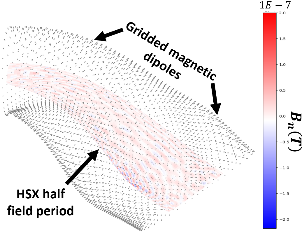
Figure 1: Example configuration of gridded magnetic dipoles on the HSX winding surface. Each dipole amplitude has been optimized to create the HSX magnetic surface. Only one field period of both the winding and magnetic surface is necessary to capture the full toroidal problem. For this case, the magnetic surface is produced with a maximal field error of $10^{-5}$%. The total field contributing to $B_{n}$ here is the toroidal $1/R$ field and the field of the magnetic dipoles.

Magnetic dipoles are placed in a grid on the HSX winding surface (see Fig. fig:3D_Dipoles+MagSurf) and are oriented normal to the winding surface. The winding surface used is the surface on which HSX’s modular coils lie. The magnetic surface used is a truncated version of HSX’s experimental equilibrium. The truncation minimizes the effect of modular coil ripple present in the equilibrium arising from the 12 coils per period of HSX. However, as discussed in Fig. fig:Bn_Fourier, this method does not entirely eliminate defects from coil ripple.

Each dipole acts as a local element to contribute magnetic field. The dipole strengths are then adjusted via a least-squares problem to minimize the normal field on the surface due to the a background toroidal field,

$$\min\bigg{(}|\mathbf{A}_{\mbox{dip}}\cdot\mathbf{x}-\mathbf{b}|^{2}\bigg{)}$$ (6)

where $\mathbf{A}_{\mbox{dip}}$, defined below, is the transfer matrix of the dipole magnetic fields, $\mathbf{x}$ represents the individual dipole strengths, and $\mathbf{b}$ represents the normal magnetic field at each point on the magnetic surface produced by external coils. In later steps, dipoles are removed entirely from the winding surface to enforce solution sparsity, or the open-access properties of the coil set.

Other sources of $B_{n}$ than a purely toroidal field were considered, for example from simple helical coils, though the results did not change significantly, neither qualitatively or numerically, and so only results from $B_{n}$ arising from a purely toroidal field are shown.

The method is motivated by the idea of a current potential with regions of high current density in some locations and low in others, or a ”sparse current potential.” Sparse current potentials are intended to have concentrated currents in the sheet which lie in small regions or thin bands. These features cannot easily be realized in a Fourier basis due to its global nature. A finite element method (FEM) basis would be ideal, in which localized patches of the current sheet can contribute independently. FEM bases support feature sharpness and so are amenable to sparsity.

Magnetic dipoles are theoretically rings of current of vanishing radius. As a result, the current of this basis is trivially divergence-free, however current cannot flow between patches. Indeed, each dipole is not a patch of current, but rather a $\delta$ function of current centered in each patch. This is the approximate nature of this basis. The surface current flowing on the winding surface is given exactly by the gradient of the current potential, which may be calculated using standard numerical methods over a grid. This approach is similar to the work done by Helander Helander_PMs:2020 . Despite this approximation, the magnetic dipole basis current potentials found agree well with Fourier basis current potentials for the same magnetic surfaces, see Sec.sec:REGCOIL_comparison.

The use of magnetic dipoles, specifically permanent magnets, to generate shaping fields is a recent approach to stellarator design Helander_PMs:2020 . In this approach, a surface or volume grid of magnetic dipoles is used to generate a given magnetic surface by varying dipole strength and orientation. These magnetic dipole methods have been improved and implemented for optimization Zhu_PMs:2020 Kaptanoglu_GPMO:2023 Hammond_PMs:2020 leading to the construction of the first permanent-magnet stellarator MUSE MUSE:2021 . Permanent magnet stellarators are remarkably able to produce magnetic surfaces to great accuracy and provide some open access, though are not viable for fusion power plants due to a variety of reasons: degradation of the magnets from neutron flux and the low field strength of the magnets if they are placed behind shielding.

Here we will describe how to initialize the magnetic dipole configurations using the winding surface. The winding surface may be represented as a surface $\mathbf{S}_{w}(\theta,\zeta)$ with a mesh grid separated uniformly in $\theta$ and $\zeta$. The magnetic dipole winding surface then consists of $n_{\theta}$ by $n_{\zeta}$ points, each of which is populated by a single magnetic dipole.

The field generated by each magnetic dipole on a plasma magnetic surface $\mathbf{S}_{p}$ at the $i$th point on the surface $\mathbf{S}_{p,i}$ is

$$\mathbf{B}(\mathbf{S}_{p,i})=\dfrac{3\hat{\mathbf{r}}(\mathbf{m}_{j}\cdot\hat{\mathbf{r}}-\mathbf{m}_{j})}{|\mathbf{r}|^{3}}$$

where $\mathbf{r}=\mathbf{x}_{j}-\mathbf{S}_{p,i}$, $\hat{\mathbf{r}}=\mathbf{r}/|\mathbf{r}|$, $\mathbf{x}_{j}$ is the position of the $j$th dipole, and $\mathbf{m}_{j}$ is the $j$th magnetic dipole vector. The inductance matrix is accordingly

$$\mathbf{A}_{\mbox{dip}}=\begin{bmatrix}\dfrac{3\hat{\mathbf{r}}_{11}(\mathbf{m}_{1}\cdot\hat{\mathbf{r}}_{11}-\mathbf{m}_{1})}{|\mathbf{r}_{11}|^{3}}&\dfrac{3\hat{\mathbf{r}}_{21}(\mathbf{m}_{2}\cdot\hat{\mathbf{r}}_{21}-\mathbf{m}_{2})}{|\mathbf{r}_{21}|^{3}}&...\\ \dfrac{3\hat{\mathbf{r}}_{12}(\mathbf{m}_{1}\cdot\hat{\mathbf{r}}_{12}-\mathbf{m}_{1})}{|\mathbf{r}_{12}|^{3}}&...&...\\ ...&...&...\\ \end{bmatrix}$$

which is an $N\times M$ matrix where $N$ is the number of evaluation points on the magnetic surface and $M$ is the number of dipoles used. Stellarator symmetry may be used to account for each dipole’s contribution from being mapped toroidally. As a result, only a half-field-period winding surface with a half-field-period of plasma surface need be considered when solving for the magnetic dipole strengths.

IV Results

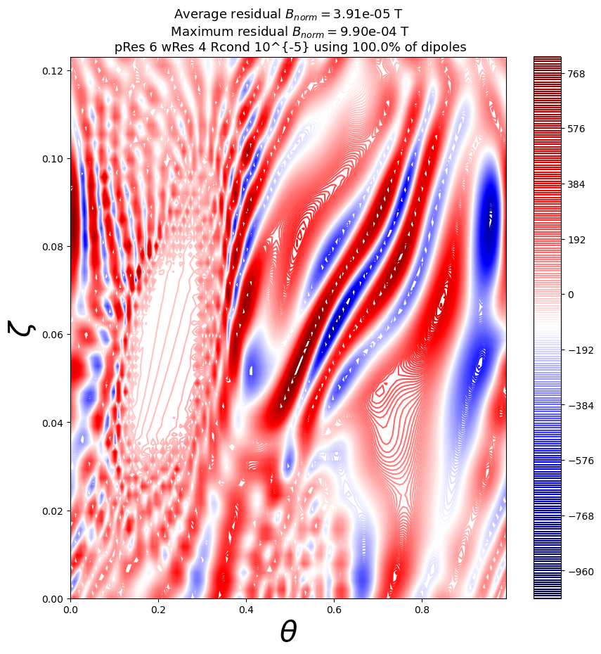
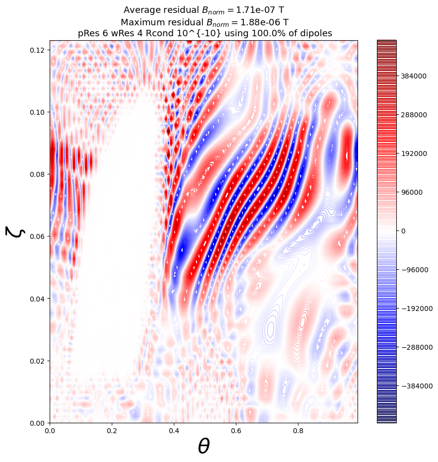
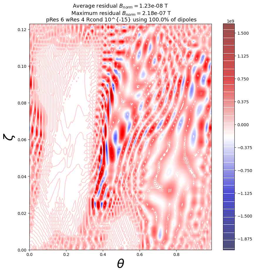
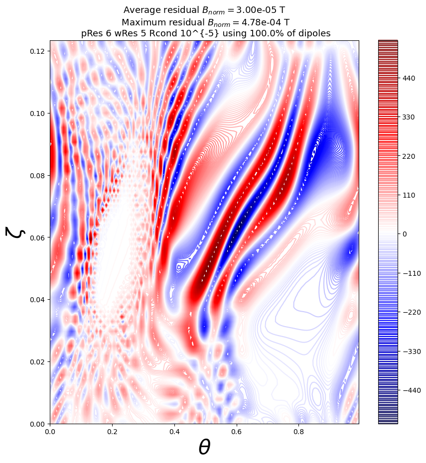
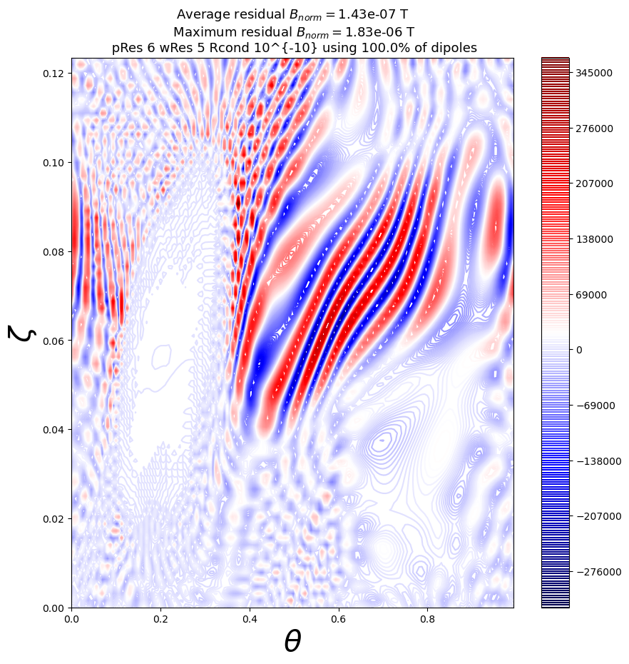
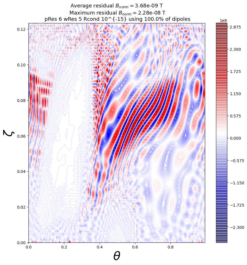
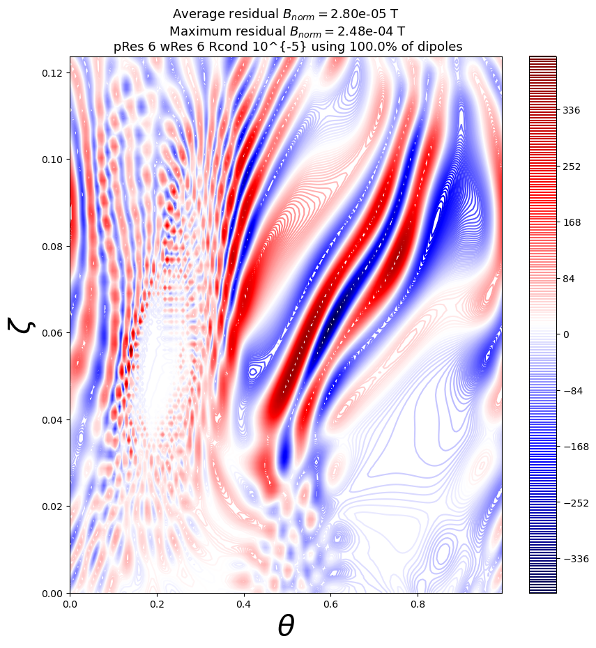
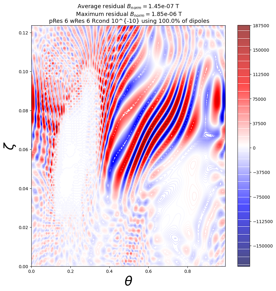
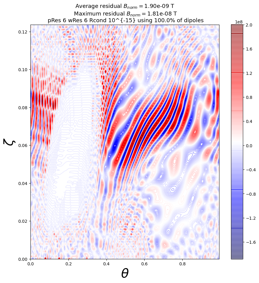
Figure 2: Surface plot of magnetic dipole amplitudes $m$ on one half field period of the HSX winding surface for a background toroidal field, analogous to the current potential $\Phi$. From left to right the dipole amplitudes are SVD-regularized with cutoff threshold $10^{-5}$, $10^{-10}$, $10^{-15}$ corresponding to limits on the maximum dipole amplitudes. For reference, SVD-regularization of the order $10^{-5}$ corresponds to dipoles 10x stronger than permanent magnets. pRes refers to plasma surface resolution, while wRes refers to winding surface resolution. From top to bottom the dipole density increases as grids of 128x64, 160x80, and 192x86 magnetic dipoles. The highest-resolution cases best-represent an actual current potential. In the bottom three figures, we see high-current-density regions appearing as large windowpane contours. Current flows along contours of constant current potential so provide initial guesses for windowpane coils.

IV.1 Winding surface solutions without sparsity promotion

The density of magnetic dipoles on the surface influences the error field significantly. As we populate the winding surface with more and more dipoles ($n\to\infty$), the discrete set of dipoles approximates a continuous FEM basis. The effect of this increasing density can also be seen in Fig. fig:Dipole_CPs_Full_WS. The physical interpretation of this effect is that higher dipole densities can support shorter-wavelength Fourier spectra.

To begin, eqn. eqn:CP_LS_problem is solved using the full HSX winding surface with different dipole densities on the surface $n_{d}$ and levels of singular value decomposition (SVD) truncation. Here, SVD regularization is the suppression of singular values of eqn:CP_LS_problem less than some cutoff parameter $r_{\mbox{cond}}$. The effect of these two parameters may be seen in Fig. fig:Dipole_CPs_Full_WS. Greater dipole densities $n_{d}$ allow the formation of high-wavenumber features in the current potential. SVD regularization limits the maximal amplitude of individual dipoles and forces solutions to be smooth by cutting off inefficient modes, see Sec. sec:SVD_fractional_regularization for more on this.

A closer inspection of the condition number of the inductance matrix reveals the tendency for high-m harmonics to arise in the current potential. The condition number of eqn:Dipole_inductance_matrix when using a grid of 128 toroidal cells by 192 poloidal cells is $\sim 10^{20}$, suggesting these solutions are very sensitive to perturbations and so the problem must be posed in such a way that the condition number is small. Thus, while these full-winding-surface-solves reveal qualities of the dipole basis, feasible coil sets must be generated using a direct SVD-truncation technique, Sec. sec:SVD_fractional_regularization.

IV.1.1 Sparsity through $L0$ regularization and SVD truncation of current potential patches

Figure 3: Fourier decomposition of Bn on the magnetic surface due to a toroidal flux. At 0.1% field accuracy, the magnetic surface quality becomes ”good enough” as a rough measurement. Interestingly, the HSX equilibrium used has some very high mode number harmonics, likely due to this equilibrium not being the original stage-1 result of HSX which has been lost. The importance of this high-mode harmonic to the equilibrium recreation could introduce significant complexity into the corresponding current configurations.

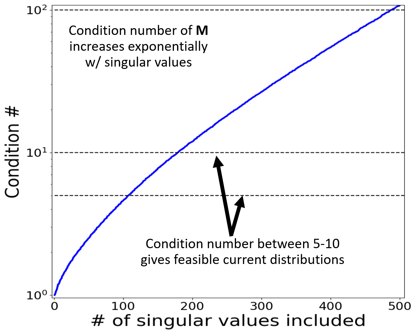
Figure 4: Condition number of the dipole-basis transfer matrix. As expected, it increases exponentially with the number of singular values included. Condition numbers between 5-10 are expected to give feasible current distributions which produce the field with sufficient accuracy to recover solution sparsity.

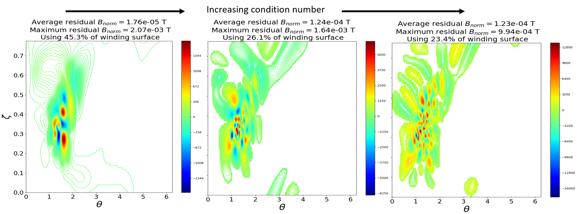
Figure 5: SVD-truncated dipole-basis current potentials. The chosen condition numbers are 10,20, and 30. Solution sparsity is achievable but there is interestingly still high ripple in the solutions. However, these features correspond to low current density regions and so are perhaps more feasible current arrangements. Conversely, current potentials with high condition numbers involve large regions of high current density, a less feasible current arrangement.

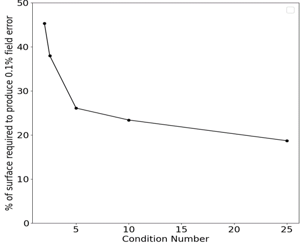
Figure 6: Fraction of surface area required to produce the equilibrium to 0.1% accuracy for different condition numbers of M. As complexity of M increases, more solution sparsity emerges. However, the saturation of the fractional surface required to produce good-quality magnetic surfaces with respect to matrix condition number provides estimate limits for open-access properties of the coil set. The level of access achieved before saturation is unique to each equilibrium.

The method that follows is closely related to the efficient field distributions method of EFDs:2016 , though this implementation uses the unique ability of current potential patches to construct discontinuous current sheets. A given normal magnetic field $B_{n}(\mathbf{x})$ on the plasma surface may be Fourier decomposed as $B_{n}(\mathbf{x})=b_{k}(\theta,\zeta)$ where

$$b_{k}(\theta,\zeta)=\sum_{m,n}^{k}b_{m,n}\cos(m\theta-n\zeta)$$ (7)

where the truncation value $k$ is determined by the maximum tolerable field error.

Exponential convergence of the Fourier series allows us to choose a Fourier truncation value $k$ such that the maximal error $\delta$ between the normal field and its Fourier representation is $|B_{n}-b_{k}|^{2}<\delta$. This Fourier representation for a certain $\delta$-quality magnetic surface tells us the efficiency with which it can be produced by a grid of magnetic dipoles on some external surface,

$$\mathbf{M}\cdot\mathbf{d}=\mathbf{b}_{k}$$ (8)

and the singular value decomposition of $\mathbf{M}$ informs the efficiency of the dipoles,

$$\mathbf{M}=\mathbf{U}\cdot\mathbf{S}\cdot\mathbf{V}^{\dagger}$$ (9)

$\mathbf{U}^{\dagger}\mathbf{d}$ relates which distributions of dipoles are most efficient at producing Fourier components, while $\mathbf{V}^{\dagger}\cdot\mathbf{b}_{k}$ relates which magnetic fourier terms are easily produced by the dipoles. $\mathbf{M}$ is similar to the transfer matrix $\mathbf{A}$ but instead of relating the magnetic field of magnetic dipoles to points on the magnetic surface, $\mathbf{M}$ relates point dipoles to Fourier-decomposed normal magnetic field distributions on the magnetic surface.

The condition number of $\mathbf{M}$ is given by the ratio of the largest to smallest singular values of $\mathbf{S}$. If the condition number is high, then inefficient components of the dipole field are being used to produce the field on the surface. As long as the condition number is low, say $10^{0}-10^{1}$, the dipoles are used efficiently and the resulting current potentials are more feasible.

We apply this analysis technique to the HSX equilibrium. The Fourier representation of $B_{n}$ eqn:Bn_Fourier may be seen in Fig. fig:Bn_Fourier. The condition number of the associated matrix $\mathbf{M}$ from eqn:M_SVD may be found in Fig. fig:CondNumber.

We enforce sparsity through the following method: eqn:M_SVD is truncated of singular values up to a given condition number, which is then solved via a least-squares problem eqn:Dipole_Bn_efficiency_discussion, then sparsity is enforced by removing all dipoles with strengths less than some threshold strength $m_{dip}$ from the winding surface. Finally, the remaining dipole strengths are adjusted through another least-squares solved using only the remaining dipoles place on the winding surface. In this way, we may use small coverage regions of the current potential surface to produce the desired equilibrium while maintaining a low matrix condition number.

Example truncated-SVD current potentials may be found in Fig. fig:Money1. The more efficient locations of current placement coincide wihh low current density regions of the current potential. In Fig. fig:Dipole_CPs_Full_WS, these are the whitish regions of the current potential. The implication coincides with a general feature of efficient fields: inefficient fields are produced using short-wavelength, high current density features in the current potential.

IV.2 Comparison with REGCOIL

We compare the current potential patch results with single-valued current potentials in the Fourier basis, fig:REGCOIL_SV_CPs. Each current potential shown produces the HSX magnetic surface to similar levels of error to the figures found in Fig. fig:Dipole_CPs_Full_WS using different levels of Tikhonov regularization. In this case, Tikhonov regularization uses the $L2$ norm of the current density, which is the REGCOIL formulation REGCOIL:2017 . The Fourier-basis current potentials do remarkably well in producing sparse features, likely due to the high toroidal and poloidal mode numbers allowed in the current potential. Even so, these results suggest strong localization of current can be achieved with fourier-basis current potentials.

V Summary

A novel method to investigate access properties of stellarator coil sets was developed. The tool, known as current potential patches, uniquely retain the solution properties of current potentials for coil design yet are able to generate sparse solutions. An example calculation using the HSX winding and magnetic surfaces demonstrates the ability of current potential patches to (i) identify crucial locations of current placement for surface shaping, for example using windowpane coils and (ii) provide an example bounding calculation on a coil set with maximal open-access properties which still produces the desired magnetic surface to a given degree of accuracy. This method could be applied to (iii) the generation of localized windowpane coils for error field remediation or the use of a coilset consisting of simple modular or helical coils to provide the bulk toroidal field and windowpane coils to provide the rest. Overall, this method has use in stellarator design in which access to the vacuum vessel and region interior to the coil set is desired.

The access limits set by the method are approximate due to the use of surface currents. The use of filamentary coils would likely decrease access properties due to the inability of filamentary coils to produce the current distributions of current sheets.

This method has a few direct applications. For one, coil sets consisting of simple toroidal field coils or helical coils in conjunction with windowpane coils can be generated using this method. In this case, contours of $\Phi_{SV}$ are the contours of windowpane coils. Second, a metric describing the amenability of an equilibrium to open-access coil sets could be derived. Further, equilibria which support good access properties could be simpler by not relying on complicated shaping currents throughout the winding surface to support them.

Appendix A Single-valued current potential and dipoles

The single-valued part of the current potential $\Phi$ in a small region on a surface can be represented by a magnetic dipole. Let $\hat{z}$ be the normal to the surface and use cylindrical coordinates. The magnetic moment analog of a current density is

$$\vec{m} = \frac{1}{2}\int r\hat{r}\times\vec{j}d^{3}x,\mbox{ and }$$ (10)

$$\vec{j} = (\vec{\nabla}\kappa\times\hat{z})\delta(z),\mbox{ so }$$ (11)

$$\vec{m} = -\frac{\hat{z}}{2}\int r\frac{\partial\kappa(r,\theta)}{\partial r}\delta(z)rdrd\theta dz$$ (12)

$$= -\frac{\hat{z}}{2}\int r^{2}\left(\int_{0}^{2\pi}\frac{\partial\kappa(r,\theta)}{\partial r}d\theta\right)dr$$ (13)

$$= -\frac{\hat{z}}{2}\int 2\pi r^{2}\bar{\kappa}(r)dr$$ (14)

$$= -\pi\hat{z}\int\Big{(}\frac{d}{dr}(r^{2}\bar{\kappa})-2r\bar{\kappa}dr$$ (15)

$$= \hat{z}\int\kappa(r,\theta)rdrd\theta,$$ (16)

where $2\pi\bar{\kappa}\equiv\int_{0}^{2\pi}\kappa(r,\theta)d\theta$. Since $(\hat{r}\times\hat{\theta})\cdot\hat{z}=1$, $\hat{r}\times(\vec{\nabla}\kappa\times\hat{z})=-\hat{z}\partial\kappa/\partial r$. The current potential $\kappa(r,\theta)$ is assumed to be zero outside of the region of the radial integration. The area element for this patch on the surface is $da=rdrd\theta$.

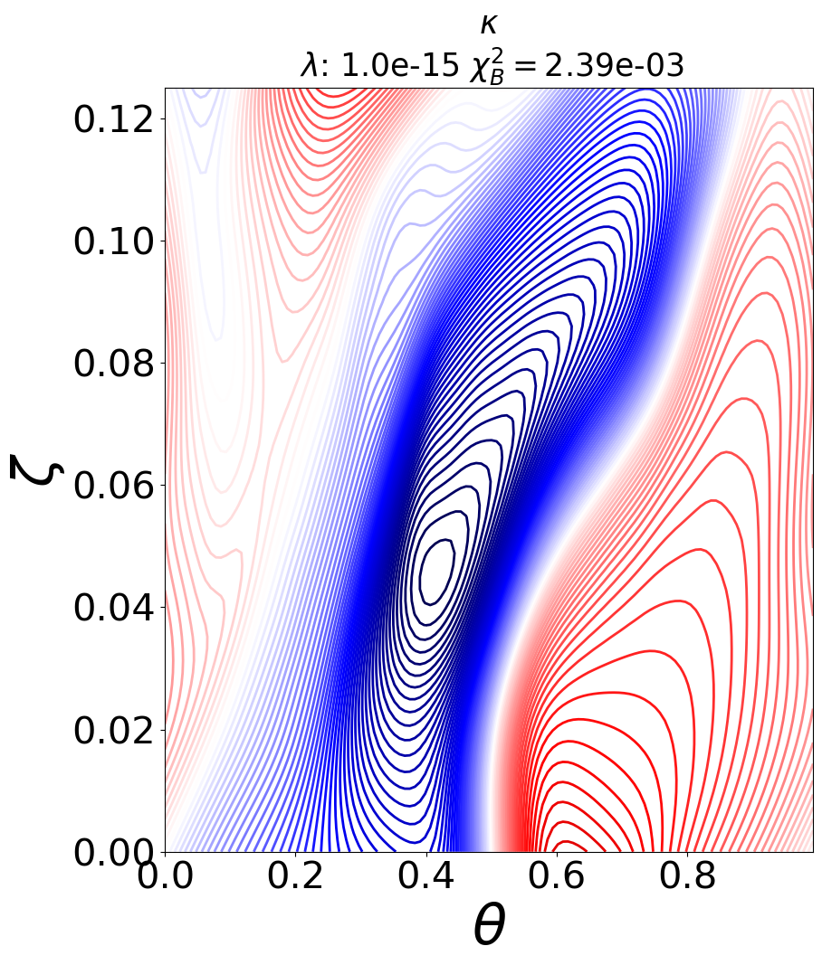
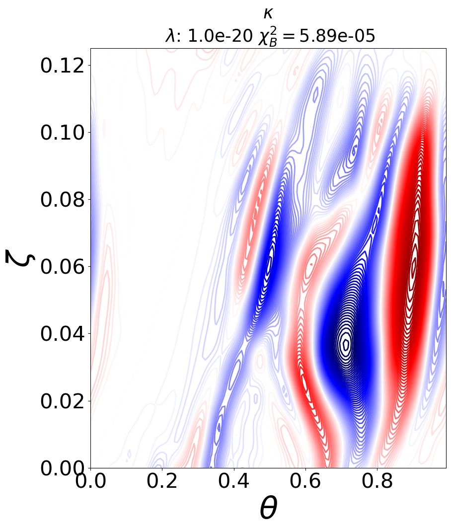
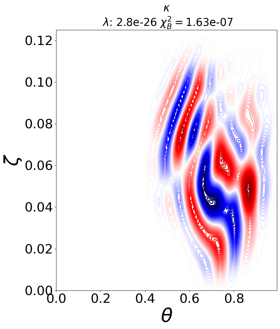
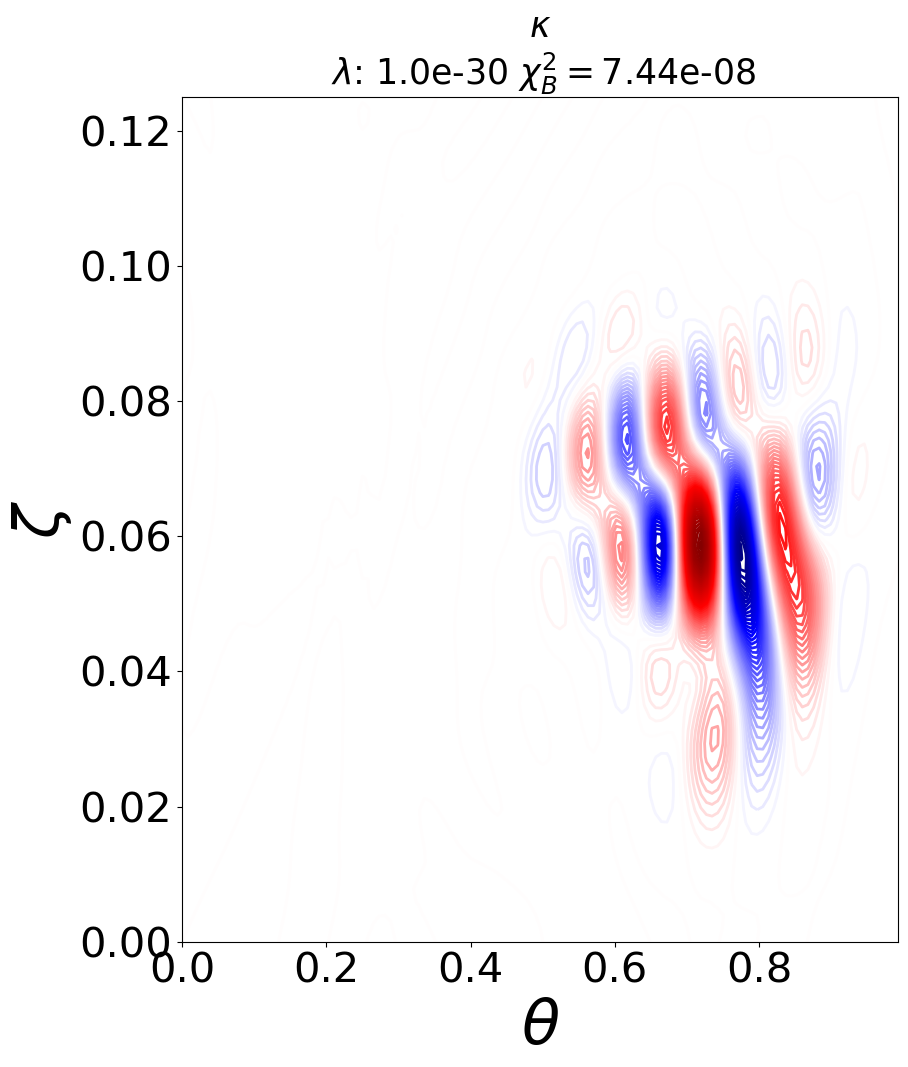
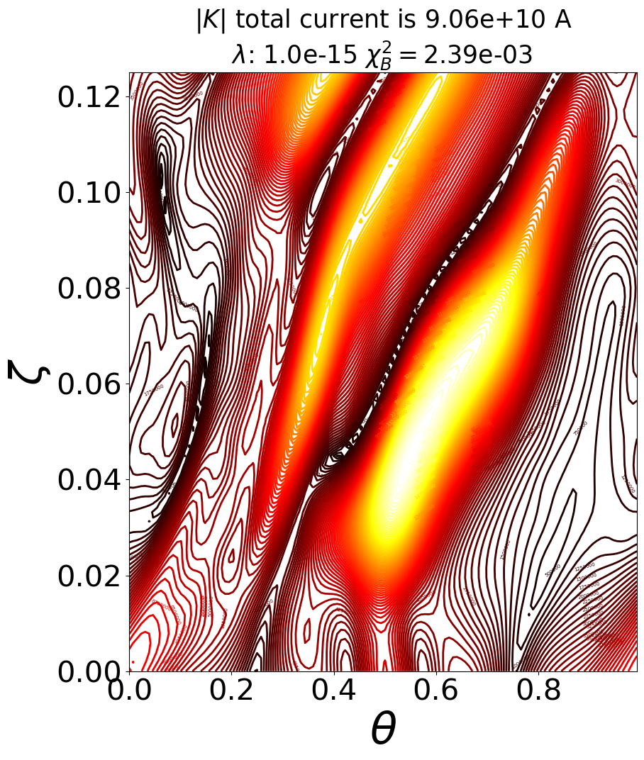
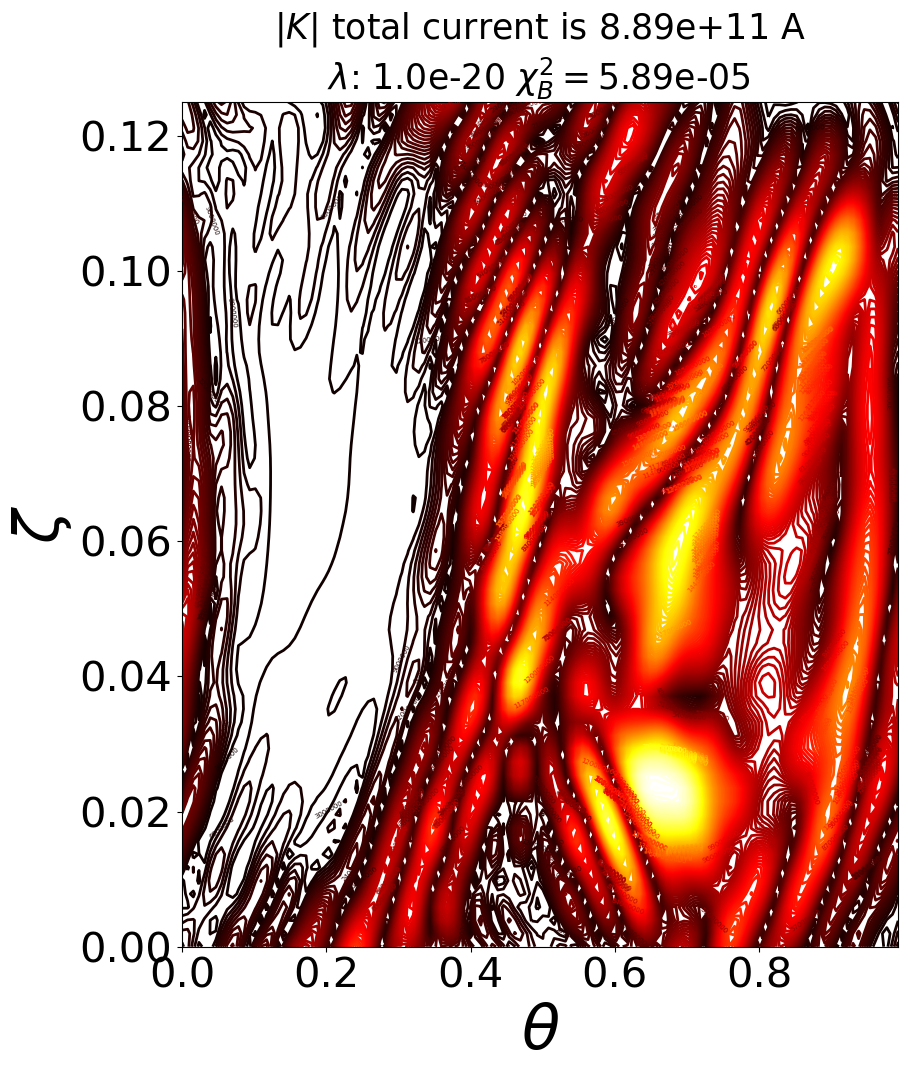
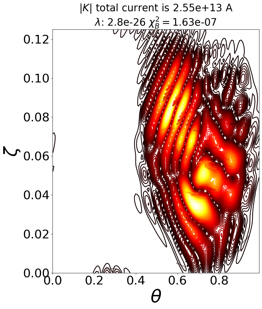
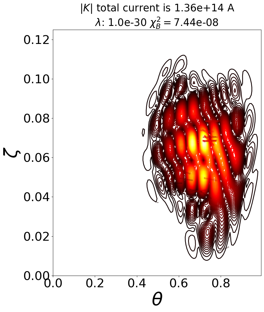
Figure 7: Single-valued fourier-basis current potentials computed by REGCOIL, each with a different level of Tikhonov regularization. The top figures are $\Phi_{SV}$ while the bottom are $|K|$. The title of each figure denotes the integrated current density $|K|$, amount of Tikhonov regularization $\lambda$, and average $|B_{n}|$ error. These current potentials were generated using a grid of 64 poloidal points and 32 toroidal points per half field period, and a maximum poloidal and toroidal mode number of 14. Remarkably, the dipole basis produces similar qualitative results to that of Fig. 2: the high current density locations are similarly localized and have high ripple.

References

- (1) S. I. Krasheninnikov and A. S. Kukushkin, Physics of ultimate detachment of a tokamak divertor plasma, Journal of Plasma Physics, 83, 155830501 (2017).
- (2) TS Pedersen et. al., Confirmation of the topology of the Wendelstein 7-X magnetic field to better than 1:100,000, Nature communications, 7 1, 13493 (2016).
- (3) C Zhu et. al., Towards simpler coils for optimized stellarators, IAEA Conference, (2018).
- (4) S. Rehker and H. Wobig, Stellarator Fields with Twisted Coils, IPP 2/215 , (1973).
- (5) P. Merkel, Solution of stellarator boundary value problems with external currents, Nuclear Fusion, 27, 867 (1987).
- (6) M. Landreman, An improved current potential method for fast computation of stellarator coil shapes, Nuclear Fusion, 57, 046003 (2017).
- (7) Allen H Boozer, Physics of magnetically confined plasmas, Reviews of modern physics, 76 4, 1071-1141 (2005)
- (8) AH Boozer, Stellarator design, Journal of Plasma Physics, 81 6, 515810606 (2015).
- (9) M. Landreman and AH Boozer, Efficient magnetic fields for supporting toroidal plasmas, Physics of Plasmas, 23, 032506 (2016).
- (10) D. Lazanja, Components of the magnetic field from interior and exterior sources in toroidal geometry, Columbia University PhD thesis, (2011).
- (11) T. Askham and A.J.Cerfon, An adaptive fast multipole accelerated Poisson solver for complex geometries, Journal of Computational Physics, 304, 1-22 (2017).
- (12) Caoxiang Zhu et al Designing stellarators using perpendicular permanent magnets Nucl. Fusion 60, 076016 (2020).
- (13) P. Helander et. al., Stellarators with Permanent Magnets, Physical Review Letters, 124, 095001 (2020).
- (14) AA Kaptanoglu, GP Langlois, M Landreman, Topology optimization for inverse magnetostatics as sparse regression: application to electromagnetic coils for stellarators, Computer Methods in Applied Mechanics and Engineering, 418A, 116504 (2023).
- (15) K.C. Hammond et. al., Geometric concepts for stellarator permanent magnet arrays, Nuclear Fusion, 60, 106010 (2020).
- (16) M. Zarnstorff et. al., MUSE: A Simple Optimized Stellarator Using Permanent Magnets, APS DPP conference (2021).