Prequantisation from the path integral viewpoint

Abstract

The quantum mechanically admissible definitions of the factor $\exp\big{[}(i/\hbar)S(\gamma)\big{]}$ in the Feynman integral are put in bijection with the prequantisations of Kostant and Souriau. The different allowed expressions of this factor – the inequivalent prequantisations – are classified. The theory is illustrated by the Aharonov-Bohm experiment and by identical particles.

I Introduction

In HPAix79 an attempt was made to use the geometric techniques of Kostant and Souriau Kostant ; SSD (“K-S theory”) to study path integrals. The method was then applied to a Dirac monopole and to the Aharonov-Bohm experiment. In this note we generalize those results. We show indeed that a general symplectic system is quantum mechanically admissible (Q.M.A.) iff it is prequantisable in the Kostant-Souriau sence Kostant ; SSD ; SimmsWoodhouse with transition functions which depend only on space-time variables.

If the configuration space is not simply connected, then a given classical system may admit different, inequivalent quantisations , implied by inequivalent prequantisations. The main result is the content of in Theorem 3 announced in sec.IV, obtained by spelling out the classification scheme implicitly recognised by Kostant Kostant , and by Dowker DowkerAustin , is illustrated in FIG.1. Its proof ackKollar is presented in the Appendix.

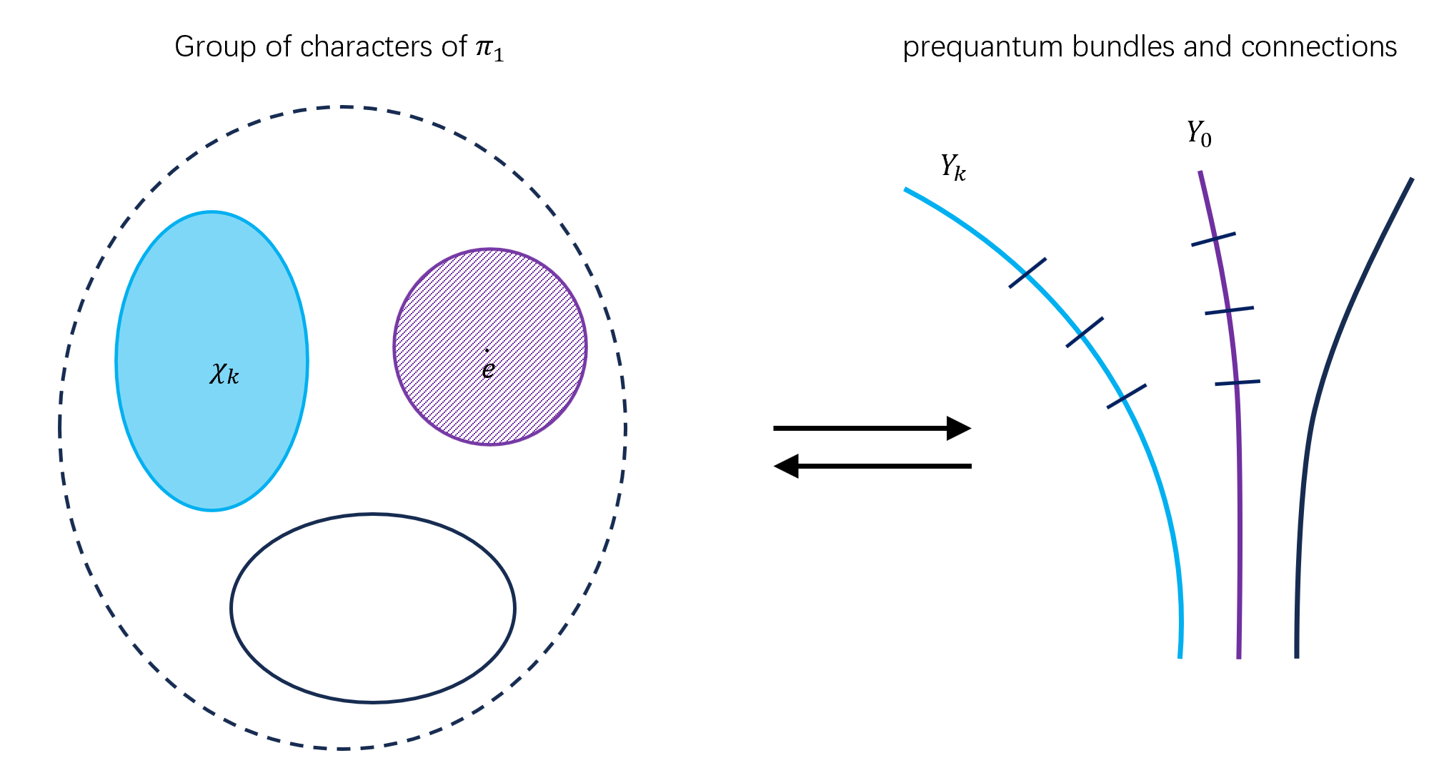
Figure 1: In $d\geq 3$ spatial dimensions, the inequivalent quantisations correspond to the characters of the fundamental group of the configuration space, $\pi_{1}(Q)$, (IV.4). The topologically distinct bundles correspond to the components of the character group and can be labelled by choosing (non canonically) a character $\chi_{i}$ in its respective component. The inequivalent connections on a chosen bundle are in bijection with the characters in the identity component which correspond physically to curl-less “Aharonov-Bohm - type” vector potentials.

The fundamental concept is the “Feynman factor”

$$\mathcal{F}(\gamma)=\exp\left[\hbox{$\textstyle\frac{i}{\hbar}$}S(\gamma)\right]\,,$$ (I.1)

where $S(\gamma)$ is the classical action calculated along the path $\gamma$.

The aim of this note is to provide physicists with an introduction to (geometric) prequantisation and to contribute to its physical interpretation SimmsWoodhouse ; SimmsAix79 .

II Quantum mechanically Admissible (Q.M.A.) Systems

Let us restrict ourselves to classical system $(E,\sigma)$ with evolution space $E=T^{*}Q\times{\mathds{R}}$, where $Q$ is the configuration space (where we follow Souriau’s framework SSD ). $E$ is endowed with a presymplectic structure of the form

$$\sigma=d\theta_{0}+e{\mathds{F}}\,,$$ (II.1)

where $\theta_{0}$, obtained by restricting the canoncial $1$-form of $T^{*}(Q\times{\mathds{R}})$ to the energy surface $H=H_{0}(q,p,t)$ , describes a free system SimmsWoodhouse ; SimmsAix79 . ${\mathds{F}}$, a closed $2$-form on space-time $X=Q\times{\mathds{R}}$, represents the external electromagnetic field to which our particle is coupled by the constant $\underline{e}$ SSD .

If the system admits a Lagrangian, then $\sigma=d\theta$ where $\theta$ is the Cartan form of the variational system SSD ; HPAix79 . The Hamiltonian action is obtained by integrating alongs paths $\gamma$ in phase (more precisely in evolution) space, whose initial and final points project to the same $x=(q,t)$ and $x^{\prime}=(q^{\prime},t^{\prime})$ in space-time $X$ in the Feynman factor (I.1),

$$S(\gamma)=\int_{\gamma}\theta\,.$$ (II.2)

Definition 1.

$(E,\sigma)$ is quantum mechanically admissible (Q.M.A.) system iff $E$ can be covered by a collection $\left\{U_{j},\,\theta_{j}\right\}$ of pairs of contractible open subsets $U_{j}$ and $1$-forms $\theta_{j}$ defined on them such that for any $\gamma\subset U_{j}\cap U_{k}$ we have,

$$\exp\left[\hbox{$\textstyle\frac{i}{\hbar}$}\int_{\gamma}\theta_{j}\right]=C_{jk}(x,x^{\prime})\exp\left[\hbox{$\textstyle\frac{i}{\hbar}$}\int_{\gamma}\theta_{k}\right]\,,$$ (II.3)

where the unitary complex factors $C_{jk}$ depend only on the initial and end points $x,\,x^{\prime}$ of $\gamma$ but not on $\gamma$ itself.

When (II.3) is satisfied, then the Feynman factors (I.1) which correspond to $\theta_{j}$ resp $\theta_{k}$ are related by unobservable phase factors. The idea comes from recalling that adding a total derivative to the Lagrangian (which amounts to adding an exact $1$-form to the Cartan form $\theta$) changes both $\mathcal{F}$ and the wave function by an unobservable phase factor HPAix79 .

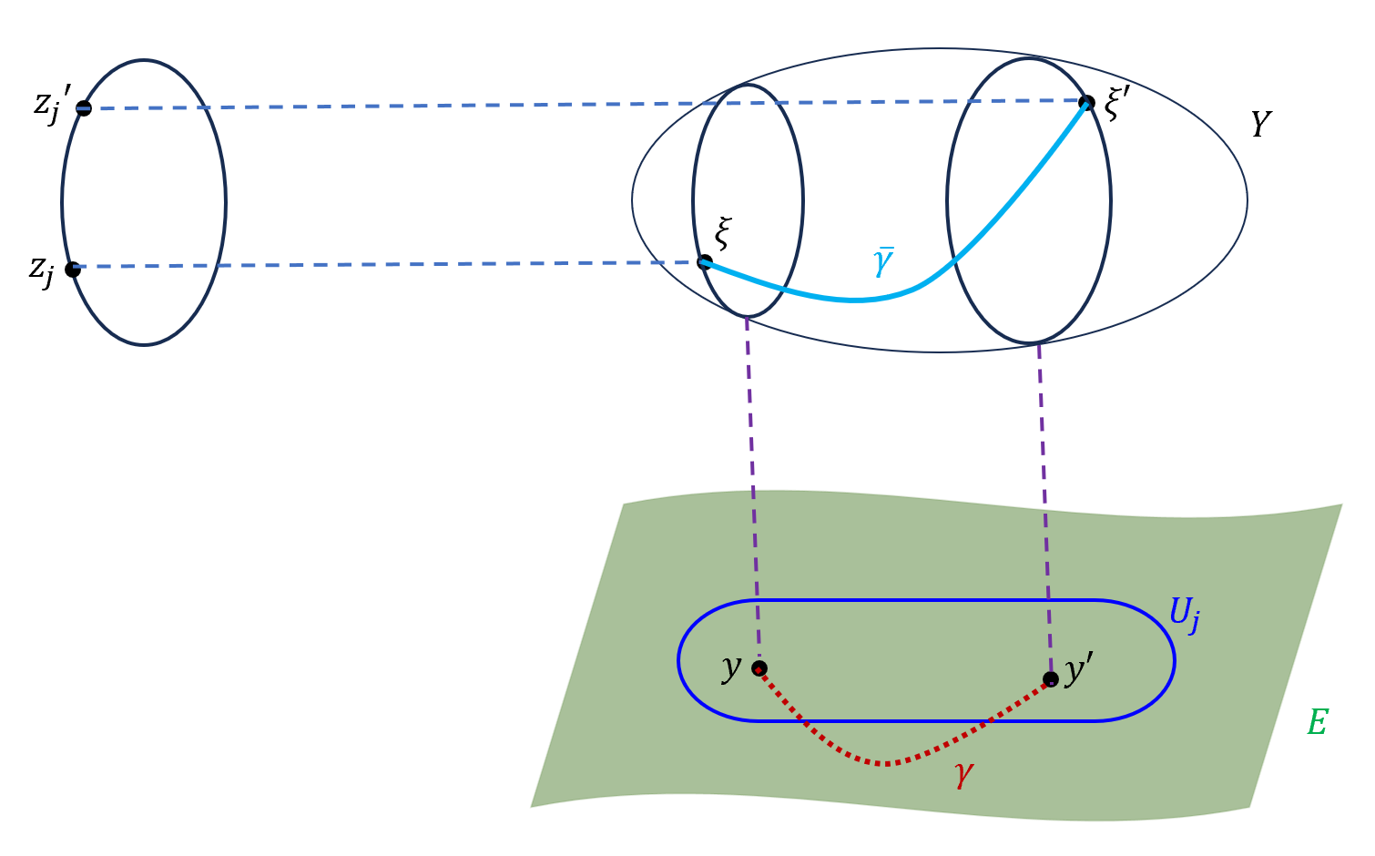
Figure 2: The Feynman factor (I.1) for a path $\gamma$ whose initial and end points $y,\,y^{\prime}$ (but necesarilly the entire $\gamma$) belong to a chosen contractible subset $U_{j}$, is defined by lifting $\gamma$ horizontally to the prequantum bundle $Y$ as $\bar{\gamma}$ and then reading off from the change of the vertical coordinate in a local trivialisation HPAix79 ; SimmsAix79 .

By the Weil lemma the consistency condition (II.3) is equivalent to requiring that the system be prequantisable Kostant ; SSD ; SimmsWoodhouse ,

$$\frac{1}{2\pi\hbar}\int_{S}\sigma\in{\mathds{Z}}$$ (II.4)

for any $2$-cycle $S$ in space-time .

The bundle framework allows us to define the Feynman factor (I.1) is any curve $\gamma$. To this end, we proceed as follows. The transition functions of the $\mathrm{U}(1)$ bundle $Z_{jk}:U_{j}\cap U_{k}\to U(1)$ satisfy, with the locally defined Cartan forms,

$$\theta_{j}-\theta_{k}=\frac{dZ_{jk}}{iZ_{jk}}{\quad\Rightarrow\quad}C_{jk}(x,x^{\prime})=\frac{Z_{jk}(x)}{Z_{jk}(x^{\prime})}\,.$$ (II.5)

Let $\gamma$ be any path in $E$ joining $y$ and $y^{\prime}$  see FIG. 2.

Denote by $\big{(}Y,\omega,\pi\big{)}$ a prequantization of $(E,\sigma)$ Kostant ; SSD ; HPAix79 where

$$\omega\quad\text{\small locally}\quad\omega\big{|}_{U_{j}}=\theta+\frac{dz}{iz}$$ (II.6)

is the prequantum 1-form SSD , defined by $\pi^{*}\sigma=d\omega$. Denote by $\bar{\gamma}$ the horizontal lift of $\gamma$ to $Y$, $\omega(\bar{\gamma})=0$ with $\bar{\gamma}(0)=\xi\in\pi^{-1}(y)$. In a local trivialization of the prequantum bundle, $Y\simeq U_{j}\times\mathrm{U}(1)$ SimmsAix79 ,

$$\bar{\gamma}(t)=\big{(}\gamma(t),Z(t)\big{)}{\quad\text{\small where}\quad}Z(t)=Z_{0}\exp\left[-\hbox{$\textstyle\frac{i}{\hbar}$}\,\int_{0}^{t}\!\theta_{j}(\dot{\gamma}(\tau))d\tau\right]\,.$$ (II.7)

Thus the exponential of the classical action calculated along the arbitrary path $\gamma(t),\,0\leq t\leq 1$ can be recovered from the horizontal lift as

$$\;\;\displaystyle{\mathcal{F}_{j}(\gamma)=\exp\left[\hbox{$\textstyle\frac{i}{\hbar}$}\int_{\gamma}\theta_{j}\right]=\frac{Z_{j}(y)}{Z_{j}(y^{\prime})}\,,}\;\;$$ (II.8)

where $\xi=\bar{\gamma}(y)=\big{(}y,Z_{j}(0)\big{)}$ and $\xi^{\prime}=\bar{\gamma}(y^{\prime})=\big{(}y^{\prime},Z_{j}(1)\big{)}$. In conclusion,

Theorem 1.

$(E,\sigma)$ is Q.M.A. iff it is prequantisable with transition functions depending only on the space-time, $X$. Then the Feynman factor (I.1) is defined for any curve $\gamma$ whose end points lie in a single $U_{j}$ as shown in FIG.2. The consistency relation (II.3) is satisfied.

Our approach, illustrated by FIG.2, is then analogous to that followed for monopoles, where the particle Lagrangian is singular along a “Dirac string” — which however can be cured by lifting the problem to a $\mathrm{U}(1)$ bundle HPAix79 ; WuYangLag ; BalaMarmo . This allows us to define the factor $\mathcal{F}(\gamma)$ also for paths which do not lie entirely in a fixed contractible subset $U_{j}$ by glueing together local expressions. Intuitively, the clue is that “the exponential of the action may behave better as the action itself”.

III Geometric expression for the integrand

Now we present a coordinate-free form to the integrand in Feynman’s expression. Following a suggestion of Friedman and Sorkin FriedmanSorkin , let us consider an arbitrary (not necessarily horizontal) path ${\widetilde{\gamma}}$ in $Y$ which projects onto $\gamma$. Write ${\widetilde{\gamma}}(0)=\xi\simeq(y,Z_{j}),\,{\widetilde{\gamma}}(1)=\xi^{\prime}\simeq(y^{\prime},Z_{j}^{\prime})$ for the end points, and let $\omega$ be the prequantum form (II.6).

Lemma III.1.

$$\exp\left[\frac{i}{\hbar}S_{j}(\gamma)\right]=\frac{Z_{j}^{\prime}}{Z_{j}}=\exp\left[\frac{i}{\hbar}\,\int_{{\widetilde{\gamma}}}\omega\right]\,.$$ (III.1)

The quotient of the vertical $Z$ coordinates is thus the same for all ${\widetilde{\gamma}}$ above $\gamma$.

Now remember that the wave function can be represented by equivariant complex function on $Y$, Kostant ; SSD ,

$$\psi\left(\underline{Z}_{Y}(\xi)\right)=Z\cdot\psi(\xi)\,,$$ (III.2)

where $\underline{Z}_{Y}$ denotes the action of $\mathrm{U}(1)$ on $Y$, rather then mere functions on the configuration space $Q$. The usual wave functions $\psi_{j}$ are the local representants of these objects, obtained as

$$\psi(\xi)=Z_{j}\cdot\psi_{j}(x),{\quad\text{\small where}\quad}\xi\in\pi^{-1}(U_{j})\,.$$ (III.3)

Thus we get finally the geometric expression for the time evolution,

$$\;\;\displaystyle{\left(U_{t^{\prime}-t}\psi\right)(\xi^{\prime})=\int_{Q}\displaystyle{\int_{P_{x,x^{\prime}}}}\!\!{\cal D}\gamma\exp\left[\hbox{$\textstyle\frac{i}{\hbar}$}\int_{\bar{\gamma}}\omega\right]\psi(\xi)\,,}\;\;$$ (III.4)

where $\xi={\widetilde{\gamma}}(0)$, $P_{x,x^{\prime}}=\Big{\{}\gamma\subset E,\,\gamma(0)=(x,\,\cdot\,),\,\gamma(1)=(x^{\prime},\,\cdot\,)\Big{\}}$ denotes the collection of all paths from $x$ to $x^{\prime}$. Note that when ${\widetilde{\gamma}}(1)=\xi^{\prime}$ is held fixed, then

$$\exp\left[\hbox{$\textstyle\frac{i}{\hbar}$}\int_{\bar{\gamma}}\omega\right]\psi(\xi)$$

is in fact a function of the projected curve $\gamma$ and is independent of the concrete choice of ${\widetilde{\gamma}}$ .

Remarks

1. To define the “integration measure” ${\cal D}\gamma$ is a formidable task which would exceed our scope here. An attempt within the geometric quantisation framework was made in SimmsAix79 .

2. The introduction of the bundle $(Y,\omega,\pi)$ allows for developping a generalized variational formalism FriedmanSorkin and allows to study conserved classical quantities.

IV A classification scheme

If the underlying space is not simply connected, then we may have more than one prequantisations and thus several inequivalent meanings of the factor $\mathcal{F}$ in (I.1). The general construction (actually elaborated in JMS67 ) is found in Souriau book SSD . Some details are outlined in the Appendix. Here we merely quote his main result :

Theorem 2.

The inequivalent prequantisations are in 1-1 correspondence with the characters of the first homotopy group.

In HPAix79 we rederived this theorem in the Aharonov-Bohm case from path-integral considerations, noting that we are always allowed to add to the Cartan $1$-form $\theta$ a closed but not exact $1$-form $\alpha$ , which, due to non-simply-connectedness, may change the propagator into an inequivalent one. The corresponding character of $\pi_{1}$ is then

$$\chi(g)=\exp\left[\hbox{$\textstyle\frac{i}{\hbar}$}\oint_{\gamma}\alpha\right]\,$$ (IV.1)

where $\gamma$ is a loop which represents the homotopy class of $g\in\pi_{1}$. In the Aharonov-Bohm experiment, for example, $\pi_{1}={\mathds{Z}}$ and all characters have this form.

This is however not the general situation. A physically interesting counter-example is that of identical particles SSD ; DowkerAustin .

Example. Consider two identical particles moving in $3$-space. The appropriate configuration is then Laidlaw $Q=\widetilde{Q}/{\mathds{Z}}_{2}$, where

$$\widetilde{Q}={\mathds{R}}^{3}\times{\mathds{R}}^{3}\setminus\{q_{1}=q_{2}\}$$ (IV.2)

is the two-particle configuration space with collisions excluded, whose homotopy group is $\pi_{1}={\mathds{Z}}_{2}$. The evolution space $E$ is $T^{*}{Q}\times{\mathds{R}}$ with $\sigma=d\theta_{0}^{(1)}+d\theta_{0}^{(2)}$. $\pi_{1}={\mathds{Z}}_{2}$ has two characters :

$$\chi_{1}(z)=1{\quad\text{\small and}\quad}\chi_{2}(z)=-1$$ (IV.3)

where $z$ is the interchange of two configurations, $(q_{1},q_{2})\to(q_{2},q_{1})$. Thus we have two prequantum lifts of $\pi_{1}$ and thus two prequantisations, the first of which is trivial, while the second is twisted. The first one corresponds to bosons, the second one to fermions $\chi_{2}$ is not of the form (IV.1) .

The general situation is described by the classification theorem (see the Appendix) says,

Theorem 3.

A character of $\pi_{1}$ can be written as

$$\;\;\displaystyle{\chi(g)=\exp\left[\frac{i}{\hbar}\,\displaystyle{\sum_{j=1}^{b_{1}}}\;a_{j}\!\oint_{\gamma}\alpha_{j}\right]\,\chi_{k},}\;\;$$ (IV.4)

where $g=[\gamma]$ is the homotopy class of the loop $\gamma$, $a_{j}\in{\mathds{R}}$ (defined mod $2\pi$). Here $b_{1}$ is the first Betti number Betti which counts the connections on a bundle. The characters $\chi_{k}$ label in turn the components of the character group.

At last we get the following refinement of Souriau’s theorem in JMS67 ; SSD in (A.3) :

Theorem 4.

Two prequantum bundles $Y_{\chi_{1}}$ and $Y_{\chi_{2}}$ associated to two characters $\chi_{1}$ and $\chi_{2}$ are topologically equivalent iff the latter belong to the same component of the group of characters. Two connection forms on a chosen bundle are labelled by the elements of the connected component of the identity character $\chi\equiv 1$ and correspond, physically, to curl-less “Aharonov-Bohm ” vector potentials. Two such vector potentials define equivalent connections when their fluxes $\Phi=\oint\!A$ differ by an integer multiple of $2\pi\hbar$. The general situation is illustrated in FIG.1.

For $b_{1}=1$ and $\alpha_{1}=\hbox{$\textstyle\frac{\Phi}{2\pi}$}d\phi$, we recover the description of the (Abelian) Aharonov-Bohm effect HPAix79 ; HoMoSu . For $\pi_{1}=$ Tors = ${\mathds{Z}}_{2}$ we get instead that of identical-particles in (at least) 3 space dimensions JMS67 ; SSD ; Laidlaw ; DowkerAustin ; AsoreyBoya ; HoMoSu . The Non-Abelian generalization is discussed in HP-Kollar .

Note added in 2024. This note was originally published in a conference proceedings HPClausthal . During the long years after its publication I came across several important papers related to the subject but not included in the original, rather succinct note, adressed to specialists in differential geometric methods of physics. In order to put it into wider perspectives and make it more readable to physicists, I decided to make available online. While following as much as I could the original note, I added many commentaries and explanations (in colored footnotes) as well as a considerably extended reference list [12 - 29]. I have also trasferred to an Appendix certain geometric details which do not belong to the standard toolbox of physicists.

Appendix A Classification of prequantizations

Souriau’s classification JMS67 ; SSD

Denote by $\big{(}\widetilde{E},\pi_{1},q\big{)}$ where $q$ is the projection $\widetilde{E}\to E$ the universal covering of $E$ and define $\tilde{\sigma}=q^{*}\sigma$. $\pi_{1}$, the first homotopy group of $E$, acts on $\widetilde{E}$ by symplectomorphisms.

Let us choose a reference prequantisation $\big{(}Y_{0},\omega_{0},\pi_{0}\big{)}$ of $(E,\sigma)$. As $\big{(}\widetilde{E},\tilde{\sigma}\big{)}$ is simply connected, it has a unique prequantisation $\big{(}\widetilde{Y}_{0},\widetilde{\omega}_{0},\widetilde{\pi}_{1}\big{)}$ Kostant ; SSD ; JMS67 , which can be obtained from $\big{(}Y_{0},\omega_{0},\pi_{0}\big{)}$ by pull-back as

$$\big{(}\widetilde{Y}_{0},\widetilde{\omega}_{0},\widetilde{\pi}_{1}\big{)}=q^{*}\big{(}Y_{0},\omega_{0},\pi_{0}\big{)}\,.$$ (A.1)

If $\chi=\pi_{1}\to U(1)$ is a character of the first homotopy group, then $\pi_{1}$ admits an isomorphic lift to $\big{(}\widetilde{Y}_{0},\widetilde{\omega}_{0},\widetilde{\pi}_{1}\big{)}$ of the form

$$\widehat{g}^{\chi}=\big{(}\tilde{x},\tilde{\xi}\big{)}=\Big{(}g(\tilde{x}),\underline{\chi(g)}_{Y_{0}}(\xi)\Big{)}\,,$$ (A.2)

where $g\in\pi_{1}$ and $\underline{Z}_{Y_{0}}$ denotes, as below (III.2), the action of $Z\in U(1)$ on $Y_{0}$ . Now Souriau has shown that

$$\big{(}Y_{\chi},\omega_{\chi},\pi_{\chi}\big{)}=\big{(}\widetilde{Y},\widetilde{\omega},\widetilde{\pi}\big{)}/\hat{\pi}_{1}^{\chi}\,$$ (A.3)

is a prequantisation of $(E,\sigma)$, and that all prequantisations are obtained in this way which proves Proposition 2:

The inequivalent prequantisations are in 1-1 correspondence with the characters of the first homotopy group.

A general scheme ackKollar

Now we outline the proof of the general classification Theorem 4.

Proposition 1.

If the homotopy group is finite, $|\pi_{1}|<\infty$, then $H^{1}(E,{\mathds{R}})=0$,  i.e.,  every closed $1$-form is exact.

Proof : Let $\alpha$ be a closed $1$-form on $E$, put $\tilde{\alpha}=q^{*}\alpha$. $\tilde{\alpha}=d\tilde{f}$ for $\widetilde{E}$ is simply connected. Define

$$\tilde{h}=\frac{1}{|\pi_{1}|}\sum_{g\in{\partial}_{1}}g^{*}f\,.$$

$\tilde{h}$ is invariant under $g\in\pi_{1}$ and projects thus to $h:E\to{\mathds{R}}$. But $\tilde{\alpha}=d\tilde{h}=q^{*}\alpha$, and thus $\alpha=dh$. The general situation can be treated by algebraic topology McLane . Consider the exact sequence of groups

$$0\longrightarrow{\mathds{Z}}\xrightarrow{~{}2\pi i~{}}U(1)\longrightarrow 0$$ (A.4)

giving rise to the long exact sequence

$$\hskip-22.76219pt\longrightarrow H^{1}(E,{\mathds{Z}})\xrightarrow{~{}\underset{\smile}{1}~{}}\underset{closed/exact}{H^{1}(E,{\mathds{R}})}\xrightarrow{~{}\underset{\smile}{2}~{}}\underset{characters}{H^{1}(E,U(1))}\xrightarrow{~{}\underset{\smile}{3}~{}}\underset{Chern~{}class}{H^{2}(E,{\mathds{Z}})}\xrightarrow{~{}\underset{\smile}{4}~{}}\underset{\begin{array}[]{c}curv.~{}class\\ \big{[}\sigma/2\pi\hbar\big{]}\end{array}}{H^{2}(E,{\mathds{R}})}\longrightarrow$$ (A.5)

Then we make the following observations:

1. $\sigma$ defines, by (II.4) an integer-valued element of $H^{2}_{dR}(E,{\mathds{R}})$ which, by de Rham’s theorem is just $H^{2}(E,{\mathds{R}})$.

2. The bundle topology is characterised by its Chern class which is in $H^{2}(E,{\mathds{Z}})$. Thus we have as many bundles as elements in the kernel of $\underline{4}$.

3. As $\mathrm{U}(1)$ is commutative, a character of $\pi_{1}$ depends only on $\pi_{1}/[\pi_{1},\pi_{1}]$, which is known to be $H_{1}(E,{\mathds{Z}})$. On the other hand, the Theorem of Universal Coefficients McLane p.76 yields that

   $$H^{1}(E,U(1))\simeq{\rm Hom}\Big{(}H_{1}(E,{\mathds{Z}}\big{)},U(1)\Big{)}\,.$$ (A.6)

   Thus $H^{1}(E,U(1))$ is the set of all characters which classify the different prequantisations as found by Souriau SSD .

4. Under quite general conditions, we have

   $$\begin{array}[]{lllll}H^{i}(E,{\mathds{Z}})&\simeq&{\mathds{Z}}^{b_{i}}&\oplus&\text{Tors}H^{i}\\[4.0pt] H_{i}(E,{\mathds{Z}})&\simeq&{\mathds{Z}}^{b_{i}}&\oplus&\text{Tors}H_{i}\end{array}$$ (A.7)

   where $b_{i}$ is the Betti number Betti . Tors $H^{i}$ and Tors $H_{i}$ are groups whose elements are all of finite order;

5. The kernel of the map $H^{i}(E,{\mathds{Z}})\longrightarrow H^{i}(E,{\mathds{R}})$ is just Tors $H^{i}$; the image of ${\mathds{Z}}^{b_{i}}$ is a basis in $H^{i}(E,{\mathds{R}})$;

6. Again by the Theorem of Universal Coefficients,

   $$\text{Tors}\,H^{2}(E,{\mathds{Z}})\simeq\text{Tors}\,H_{1}(E,{\mathds{Z}})\simeq\text{Tors}\,\pi_{1}/[\pi_{1},\pi_{1}]\,.$$ (A.8)

   Thus by 2.) 5.), 6.),

   Proposition 2.

   The topologically distinct prequantum bundles are labelled by the elements of the Torsion subgroup in (A.8).

7. According to 5.), the image of $H^{1}(E,{\mathds{Z}})$ in $H^{1}(E,{\mathds{R}})$ under 1.) is composed of integer multiples of a basis. Thus $H^{1}(E,{\mathds{R}})/({\rm Im})\big{(}H^{1}(E,{\mathds{R}})\big{)}\simeq(S^{1})^{b_{1}}$ and we get the exact sequence

   $$0\longrightarrow{S^{1}}\xrightarrow{b_{1}}H^{1}(E,U(1))\longrightarrow\text{Tors}H_{1}(E,{\mathds{Z}})\longrightarrow 0\,.$$ (A.9)

   Now by de Rham’s theorem, to any element of $H^{1}(E,{\mathds{R}})$ we can associate a closed $1$-form $\alpha/(2\pi\hbar)$ such that its value on $g\in H_{1}(E,{\mathds{R}})$ is

   $$\frac{1}{2\pi\hbar}\oint_{\gamma}\alpha\,,$$ (A.10)

   where the homology class of $\gamma$ is $g$.

   Next by (A.9), the image of $(S^{1})^{b_{1}}$ in $H^{1}(E,U(1))$ is composed of characters of the form

   $$\chi(g)=\exp\left[\frac{i}{\hbar}\oint_{\gamma}\alpha\right]\,.$$ (A.11)

   As $(S^{1})^{b_{1}}$ is connected and Tors $H^{2}(E,{\mathds{Z}})$ is finite, we have :

   Proposition 3.

   The characters of the form (A.11) make up the connected component which contains the character $\chi\equiv 1$.

8. Let us choose a basis of $H_{dR}^{1}(E,{\mathds{R}})$ composed of the $1$-forms $\alpha_{1},\dots,\alpha_{b_{1}}$, and pick a character $\chi_{k}\in H^{1}(E,U(1))$ in each element of Tors $H^{2}$ = Tors  $H_{1}$.

References

- (1) P. A. Horvathy, “Classical Action, the Wu-Yang Phase Factor and Prequantization,” Lect. Notes Math. 836 (1980), 67-90 doi:10.1007/BFb0089727
- (2) B. Kostant, “On certain unitary representations which arise from a quantization theory,” Conf. Proc. C 690722 (1969), 237-253 doi:10.1007/3-540-05310-7_28
- (3) J.-M. Souriau, Structure des systèmes dynamiques, Dunod (1970, © 1969); Structure of Dynamical Systems. A Symplectic View of Physics, translated by C.H. Cushman-de Vries (R.H. Cushman and G.M. Tuynman, Translation Editors), Birkhäuser, 1997. The “monopole without strings” discussions WuYangLag ; BalaMarmo are discussed also in the Prequantization Chap. V. written around 1975 for the planned but never completed revised edition of Souriau’s book.
- (4) D. J. Simms and N. M. J. Woodhouse, “Lectures on Geometric Quantization,” Lect. Notes Phys. 53 (1976), 1-166 doi:10.1007/3-540-07860-6
- (5) J.S. Dowker, “Selected topics in topology and quantum field theory,”, Austin Lectures, Jan - May 1979.
- (6) The results presented here were obtained in collaboration with J. Kollár.
- (7) M. Asorey, “Some Remarks on the Classical Vacuum Structure of Gauge Field Theories,” J. Math. Phys. 22 (1981), 179 [erratum: J. Math. Phys. 25 (1984), 187] doi:10.1063/1.524732
- (8) J. L. Friedman and R. D. Sorkin, “DYON SPIN AND STATISTICS: A FIBER BUNDLE THEORY OF INTERACTING MAGNETIC AND ELECTRIC CHARGES,” Phys. Rev. D 20 (1979), 2511-2525 doi:10.1103/PhysRevD.20.2511 J. L. Friedman and R. D. Sorkin, “A SPIN STATISTICS THEOREM FOR COMPOSITES CONTAINING BOTH ELECTRIC AND MAGNETIC CHARGES,” Commun. Math. Phys. 73 (1980), 161-196 doi:10.1007/BF01198122
- (9) D. J. Simms, “GEOMETRIC ASPECTS OF THE FEYNMAN INTEGRAL,” Lect. Notes Math. 836 (1980), 167-170 See also D. J. Simms, “Geometric Quantization and the Feynman Integral.” Contribution to: Mathematical Problems in Feynman Path Integral, 220-223.
- (10) M. G. G. Laidlaw and C. M. DeWitt, “Feynman functional integrals for systems of indistinguishable particles,” Phys. Rev. D 3 (1971), 1375-1378 doi:10.1103/PhysRevD.3.1375
- (11) S. McLane, Homology, Springer (1967)
- (12) J-M Souriau “Quantification géométrique. Applications.” Ann. Inst. H. Poincaré Sect. A (N.S.) 6 311-341 (1967)
- (13) L. Schulman, “A Path integral for spin,” Phys. Rev. 176 (1968), 1558 -1569 doi:10.1103/PhysRev.176.1558. L. S. Schulman, “Approximate topologies” J. Math. Phys. 12, 304 (1971) https://doi.org/10.1063/1.1665592
- (14) J. S. Dowker, “Quantum mechanics and field theory on multiply connected and on homogeneous spaces,” J. Phys. A 5 (1972), 936-943 doi:10.1088/0305-4470/5/7/004
- (15) L. S. Schulman, Techniques and applications of path integration, J. Wiley, N.Y. (1981)
- (16) P. A. Horvathy, “Quantization in Multiply Connected Spaces,” Phys. Lett. A 76 (1980), 11-14 doi:10.1016/0375-9601(80)90133-4
- (17) P. A. Horvathy, “Prequantisation From Path Integral Viewpoint,” Lect. Notes Math. 905 (1982), 197-206 CPT-80-P-1230.
- (18) P. A. Horvathy, G. Morandi and E. C. G. Sudarshan, “Inequivalent quantizations in multiply connected spaces,” Nuovo Cim. D 11 (1989), 201-228 doi:10.1007/BF02450240
- (19) P. A. M. Dirac, “The Lagrangian in quantum mechanics,” Phys. Z. Sowjetunion 3 (1933), 64-72
- (20) R. P. Feynman, “The principle of least action in quantum mechanics,” doi:10.1142/9789812567635_0001
- (21) R. P. Feynman and A. R. Hibbs, Quantum Mechanics and Path Integrals. McGraw-Hill, New York N.Y., (1965)
- (22) P. A. Horvathy, “AN ACTION PRINCIPLE FOR ISOSPIN,” BI-TP-82-19. Proceedings of the IUTAM-ISIMM Symposium on Modern Developments in Analytical Mechanics, Torino, 982, Atti Acad. Sci. Torino, Suppl. 117, 163-169 Accademia delle scienze (1983).
- (23) T. T. Wu and C. N. Yang, “Dirac’s Monopole Without Strings: Classical Lagrangian Theory,” Phys. Rev. D 14 (1976), 437-445 doi:10.1103/PhysRevD.14.437
- (24) A. P. Balachandran, G. Marmo and A. Stern, “Magnetic Monopoles With No Strings,” Nucl. Phys. B 162 (1980), 385-396 doi:10.1016/0550-3213(80)90346-6, A. P. Balachandran, G. Marmo, B. S. Skagerstam and A. Stern, “Supersymmetric Point Particles and Monopoles With No Strings,” Nucl. Phys. B 164 (1980), 427-444 [erratum: Nucl. Phys. B 169 (1980), 547] doi:10.1016/0550-3213(80)90520-9
- (25) https://en.wikipedia.org/wiki/Betti number
- (26) M. Asorey and L. J. Boya, “ELECTROMAGNETISM WITHOUT MONOPOLES IS POSSIBLE IN NONTRIVIAL U(1) FIBER BUNDLES,” J. Math. Phys. 20 (1979), 2327 doi:10.1063/1.524013
- (27) J. M. Leinaas and J. Myrheim, “On the theory of identical particles,” Nuovo Cim. B 37 (1977), 1-23 doi:10.1007/BF02727953
- (28) F. Wilczek, “Quantum Mechanics of Fractional Spin Particles,” Phys. Rev. Lett. 49 (1982), 957-959 doi:10.1103/PhysRevLett.49.957 Wilczek, Frank (2021). Fundamentals : Ten Keys to Reality. New York, New York: Penguin Press. pp. 89-90. ISBN 9780735223790. LCCN 2020020086
- (29) P. A. Horvathy and J. Kollar, “The Nonabelian Aharonov-Bohm Effect in Geometric Quantization,” Class. Quant. Grav. 1 (1984), L61 doi:10.1088/0264-9381/1/6/002.