An algebraic approach to gravitational quantum mechanics

Abstract

Most approaches towards a quantum theory of gravitation indicate the existence of a minimal length scale of the order of the Planck length. Quantum mechanical models incorporating such an intrinsic length scale call for a deformation of Heisenberg’s algebra resulting in a generalized uncertainty principle and constitute what is called gravitational quantum mechanics. Here we adopt the pseudo or g-calculus to study various models of gravitational quantum mechanics. The free time evolution of a Gaussian wave packet is investigated as well as the spectral properties of a particle bound by an external attractive potential. Here the cases of a box with finite width and infinite walls, an attractive potential well of finite depth and a delta-like potential are considered.

Keywords: Quantum gravity, Generalized uncertainty principle, Pseudo calculus

1 Introduction

In the early 20th century, physics has seen the advent of two fundamental theories, the general relativity being the contemporary theory describing the gravitational force, and the quantum theory being the basis for the description of the electro-weak and strong interactions. Quantum gravity is the attempt to unify both theories into a more fundamental one. Despite the many attempts for such a unification no consistent quantum-gravity theory could be formalised for the time being. In fact, to the best of our knowledge, the first attempt was made by Bronstein in 1936 [1]. Bronstein already concluded that there must be a minimal length in such a theory. Some 10 years later, in 1947, Snyder [2] arrived at the same conclusion by assuming that space-time is not a continuum but discrete. Lorentz invariance then let him to the conclusion that the usual Heisenberg commutation relation of position operator $\hat{X}$ and momentum operator $\hat{P}$ calls for a deformation of the form

$$[\hat{X},\hat{P}]={\rm i}(1+\beta\hat{P}^{2})\,.$$ (1)

Here and throughout this paper we will use units where $\hbar=1$. In the above $\beta>0$ represents the deformation parameter which, in our units, has the dimension of an area. Hence, for simplifying notation we will also use the alternative parameter $\lambda=\sqrt{\beta}$ which has the dimension of a length. As quantum gravity effects are believed to become visible at the Planck scale this length should be of the order of the Planck length, $\lambda\sim 10^{-35}\,m$. Quantum mechanics based on above deformed Heisenberg algebra is called gravitational quantum mechanics. The deformed algebra implies the uncertainty relation

$$\Delta X\Delta P\geq\frac{1}{2}\left|\langle[\hat{X},\hat{P}]\rangle\right|=\frac{1}{2}\left[1+\lambda^{2}\langle\hat{P}^{2}\rangle\right]\,,$$ (2)

which, in the rest frame where $\langle\hat{P}\rangle=0$ and $\Delta P=\sqrt{\langle\hat{P}^{2}\rangle}$ , results in the lower bound

$$\Delta X\geq\frac{1}{2}\left[\frac{1}{\Delta P}+\lambda^{2}\Delta P\right]\,.$$ (3)

The minimal length is given by $\min\Delta X=\lambda$ where $\Delta P=1/\lambda$. Thus, to incorporate the concept of a minimum measurable length into quantum mechanics, one should deform the standard Heisenberg algebra in the form (1). The resulting uncertainty relation (2) is called Generalized Uncertainty Principle (GUP).

Since the middle of the last century an enormous amount of work has been invested in this topic resulting in a vast number of papers addressing the effects of GUP on quantum mechanical systems. There had been investigations in the high-energy regime, but also studies of black holes and their thermodynamic properties. Here we limit ourselves to refer to some more recent extensive reviews [3, 4] which provide huge lists of original references to the subject.

The purpose of this paper is to investigate the GUP algebra, that is the deformed Heisenberg algebra (1) with its generalized uncertainty principle (2), in an algebraical way. In doing so, we will present a GUP-calculus, which may be understood as a variant of the so-called non-Newtownian calculus introduced by Grossman and Katz in 1972 [5]. This non-Newtownian calculus is also known under the name of $g$-calculus [6] and has recently found some applications in studies related to dark matter and dark energy [7]. These tools are then applied to various problems in gravitational quantum mechanics.

We start with reviewing some of the known representations of the GUP algebra in section 2. Section 3 then introduces the aforementioned GUP calculus, where we discuss concepts like GUP addition and associated derivatives but also introduce the GUP integral, the GUP delta and the GUP exponential function. Continuity conditions for the GUP derivative of wave functions are found in cases where the potential has a finite discontinuity. These are then utilized in the following sections. In section 4 we study the free gravitational quantum dynamics of a Gaussian wave packet. Hereby we obtained the GUP Fourier transformation as an approximation of the standard Fourier transformation adapted to the needs of gravitational quantum mechanics. In section 5 we will look at the eigenvalue problem of the GUP Hamiltonian for the particle in a box with infinite walls and a potential well of finite depth. We also discuss the bound state generated by the GUP-delta function potential. Some final remarks are provided in section 6.

2 Representations of the GUP algebra

The GUP algebra (1) exhibits various representations, some of which we will discuss below.

GUP momentum representation:
The most natural representation is the one where the operator $\hat{P}$ is represented by a real number $P\in\mathbb{R}$. Consequently, $\hat{X}$ is then represented by a differential operator. That is, we have

$$\hat{X}={\rm i}\left(1+\beta P^{2}\right)\frac{\partial}{\partial P}\,,\qquad\hat{P}=P\,,$$ (4)

which may easily be verified to obey the GUP algebra (1). This representation was first discussed in full detail by Kempf et al [8]. They have shown that the corresponding Hilbert space ${\cal H}_{P}=L^{2}\left(\mathbb{R},{\rm d}\mu(P)\right)$ is equipped with a scalar product of the form

$$\langle\Phi|\tilde{\Phi}\rangle=\int_{-\infty}^{\infty}{\rm d}\mu(P)\,\Phi^{*}(P)\tilde{\Phi}(P)=\int_{-\infty}^{\infty}\frac{{\rm d}P}{1+\beta P^{2}}\Phi^{*}(P)\tilde{\Phi}(P)\,.$$ (5)

Here the states are represented by wave functions $\Phi(P)=\langle P|\Phi\rangle$ and $\tilde{\Phi}(P)=\langle P|\tilde{\Phi}\rangle$. The expectation values of an observable $\hat{A}$ in such state $\Phi(P)$ is given by

$$\langle\hat{A}\rangle_{\Phi}=\langle\Phi|\hat{A}|\Phi\rangle=\int_{-\infty}^{\infty}\frac{{\rm d}P}{1+\beta P^{2}}\,\Phi^{*}(P)\bigl{(}\hat{A}\Phi\bigr{)}(P)\,.$$ (6)

Let us also note that both, $\hat{P}$ and $\hat{X}$, are symmetric operators on ${\cal H}_{P}$ as was explicitly shown in [8]. The corresponding non-relativistic GUP Hamiltonian of a particle with mass $M>0$ in the presence of a real-valued scalar potential $V$ reads

$$H_{P}:=\frac{P^{2}}{2M}+V\left({\rm i}\left(1+\beta P^{2}\right)\frac{\partial}{\partial P}\right)\,.$$ (7)

For an explicit discussion of the eigenvalue problem of $H_{P}$ for the harmonic oscillator problem we refer the work by Kempf et al [8]. In going forward we will call the representation (4) the GUP momentum representation.

Canonical momentum representation:
Let us consider the standard canonical momentum representation where the momentum operator $\hat{p}$ is represented by a real number $p$ and the position operator $\hat{x}$ by the derivative $i\partial_{p}$. Obviously we have

$$\hat{x}={\rm i}\partial_{p}\,,\qquad\hat{p}=p\,,\qquad[\hat{x},\hat{p}]={\rm i}\,,$$ (8)

the standard canonical commutation relation. In terms of this canonical representation the GUP algebra is realized by the relations

$$\hat{X}={\rm i}\partial_{p}\,,\qquad\hat{P}=\frac{1}{\lambda}\tan\left(\lambda p\right)\,,$$ (9)

as can easily be verified. We will call this the canonical momentum representation of the GUP algebra. Whereas the GUP position operator $\hat{X}$ and the canonical position operator $\hat{x}$ exhibit the same realization, the corresponding momentum operators are significantly different as $\lambda P=\tan(\lambda p)$. That is, $p$ cannot take arbitrary real values but is restricted to the interval $-p_{0}<p<p_{0}$, where $p_{0}:=\frac{\pi}{2\lambda}$ represents a cutoff of the canonical momentum. The inverse map is given by the $\arctan$ function definite as the principle branch of the inverse of the tangent function, which we will denote by $\varphi$ wherever suitable,

$$p=\varphi(P):=\frac{1}{\lambda}\arctan(\lambda P)\,.$$ (10)

Noting that $\varphi^{\prime}(P)=1+\beta P^{2}$ the scalar product (5) for two wave function $\phi(p):=\langle p|\phi\rangle$ and $\tilde{\phi}(p)=\langle p|\tilde{\phi}\rangle$ changes to

$$\langle\phi|\tilde{\phi}\rangle=\int_{-p_{0}}^{p_{0}}{\rm d}p\,\phi^{*}(p)\tilde{\phi}(p)\,.$$ (11)

That is, in essence ${\cal H_{P}}$ is changed to ${\cal H}_{p}:=L^{2}([-p_{0},p_{0}],{\rm d}p)$. Expectation values of an observable $\hat{A}$ in a state represented by a wave function $\phi(p)$ are given by

$$\langle\hat{A}\rangle_{\phi}=\langle\phi|\hat{A}|\phi\rangle=\int_{-\frac{\pi}{2\sqrt{\beta}}}^{\frac{\pi}{2\sqrt{\beta}}}{\rm d}p\,\phi^{*}(p)\bigl{(}\hat{A}\phi\bigr{)}(p)$$ (12)

and the corresponding GUP Hamiltonian reads in this canonical momentum representation

$$H_{p}:=\frac{1}{2M\lambda^{2}}\tan^{2}\left(\lambda p\right)+V\left({\rm i}\partial_{p}\right)$$ (13)

GUP position representation:
Recalling the well-known relation $[\hat{x},f(\hat{p})]={\rm i}f^{\prime}(\hat{p})$ valid for any reasonable function $f$, the position representation of the GUP algebra is

$$\hat{X}=\hat{x}=x\,,\qquad\hat{P}=\frac{1}{\lambda}\tan\left(\lambda\hat{p}\right)=\frac{1}{\lambda}\tan\left(-{\rm i}\lambda\partial_{x}\right)=\frac{1}{{\rm i}\lambda}\tanh\left(\lambda\partial_{x}\right)\,.$$ (14)

When dealing with GUP quantum mechanics, one usually assumes that $\lambda$ is sufficiently small. Hence, we may express the momentum operator with the help of the Taylor series for the hyperbolic tangent, which reads

$$\tanh z=z\sum_{n=0}^{\infty}\frac{2^{2n+2}(2^{2n+2}-1)}{(2n+2)!}\,B_{2n}\,z^{2n}\,,$$ (15)

where $B_{n}$ stands for the $n$-th Bernoulli number. Hence, to first order in $\beta$ the momentum operator is given by

$$\hat{P}=-{\rm i}\partial_{x}+{\rm i}\frac{\beta}{3}\partial_{x}^{3}+O(\beta^{2})\,.$$ (16)

In this representation the inner product for two states characterised by the wave functions $\psi(x)=\langle x|\psi\rangle$ and $\tilde{\psi}(x)=\langle x|\tilde{\psi}\rangle$ is the standard product

$$\langle\psi|\tilde{\psi}\rangle=\int_{-\infty}^{\infty}{\rm d}x\,\psi^{*}(x)\tilde{\psi}(x)\,.$$ (17)

That is, here we are back on the standard Hilbert space ${\cal H}_{x}=L^{2}(\mathbb{R},{\rm d}x)$, where expectation values of observables are given in the usual way

$$\langle\hat{A}\rangle_{\psi}=\langle\psi|\hat{A}|\psi\rangle=\int_{-\infty}^{\infty}{\rm d}x\,\psi^{*}(x)\bigl{(}\hat{A}\psi\bigr{)}(x)$$ (18)

However, the corresponding GUP Hamiltonian is not a standard Schrödinger Hamiltonian as it is of the form

$$H_{x}:=-\frac{1}{2M\lambda^{2}}\tanh^{2}\left(\lambda\partial_{x}\right)+V\left(x\right)\,.$$ (19)

3 GUP-calculus

The objective of this section is to utilize ideas and concepts of the so-called $g$-calculus based on the work by Pap [6]. The interested reader may also consult ref. [5] for more details. In $g$-calculus one considers a bijection $g:\mathbb{R}\to\mathbb{D}$, where $\mathbb{D}\subseteq\mathbb{R}$. This invertible function $g$ then induces a pseudo addition and substraction defined by

$$a\oplus_{g}b:=g^{-1}\bigl{(}g(a)+g(b)\bigr{)}\,,\qquad a\ominus_{g}b:=g^{-1}\bigl{(}g(a)-g(b)\bigr{)}\,,$$ (20)

which is equivalent to

$$g\bigl{(}a\oplus_{g}b\bigr{)}=g(a)+g(b)\,,\qquad g\bigl{(}a\ominus_{g}b\bigr{)}=g(a)-g(b)\,.$$ (21)

This is the basic idea of $g$-calculus, which we will now adopt for the gravitational quantum mechanics.

GUP addition:
Let us identifying $g$ with the function $\varphi$ introduced in (10). Hence, from now on we have

$$g(z)\equiv\varphi(z)=\frac{1}{\lambda}\arctan(\lambda z)\,,\qquad\varphi^{-1}(z)=\frac{1}{\lambda}\tan(\lambda z)\,.$$ (22)

We will leave it to the reader as a little exercise to verify that

$$a\oplus_{\varphi}b=\frac{a+b}{1-\beta ab}\,,\qquad a\ominus_{\varphi}b=\frac{a-b}{1+\beta ab}\,.$$ (23)

Recall that $\beta=\lambda^{2}$. As a side remark we may note that when formally setting $\beta=-1/c^{2}$, here $c$ denotes the speed of light, the above GUP addition is identical in form with the Lorentz invariant addition of velocities.

GUP derivative:
Here let us start by defining the GUP derivative as follows

$$D_{x}:=\frac{1}{\lambda}\tanh\left(\lambda\partial_{x}\right)=-\frac{{\rm i}}{\lambda}\tan({\rm i}\lambda\partial_{x})=-{\rm i}\varphi^{-1}({\rm i}\partial_{x})\,.$$ (24)

Here we note that this definition is similar but different to the $g$-derivative as define in [6]. With this defnition the GUP Hamiltonian (19) now takes the simple form

$$H_{x}=-\frac{1}{2M}D^{2}_{x}+V\left(x\right)\,.$$ (25)

It is obvious that on ${\cal H}_{x}$ this derivative is anti-symmetric, i.e.  $D_{x}^{\dagger}=-D_{x}$. This implies that the corresponding momentum operator is symmetric, cf. (14),

$$\hat{P}=-{\rm i}D_{x}=\frac{1}{{\rm i}\lambda}\tanh\left(\lambda\partial_{x}\right)\,,\qquad\hat{P}^{{\dagger}}=\hat{P}$$ (26)

but it is not self-adjoint [10]. In fact, as we will see below, the eigenfunctions of $\hat{P}$ do not form a complete set in ${\cal H}_{x}$.

GUP integral:
At later stage we will also need the GUP integral which we define as inverse operation to the GUP derivative. Hence, for suitable functions $f$ we define

$$\int{\rm D}_{\varphi}x\,f(x):=-{\rm i}\int{\rm d}x\,\varphi({\rm i}f(x))=\frac{1}{\lambda}\int{\rm d}x\,{\rm arctanh\,}(\lambda f(x))\,,$$ (27)

which indeed obeys the relation

$$\int{\rm D}_{\varphi}x\,(D_{x}g)(x)=-{\rm i}\int{\rm d}x\,\varphi({\rm i}D_{x}g)(x))=\int{\rm d}x\,\partial_{x}g(x)=g(x)$$ (28)

for functions $g$ where above expressions are well-defined. As an application, let us considered the stationary Schödinger equation for a potential $V(x)$ being bounded but not necessarily continuous at say $x=x_{0}$ and GUP integrate it over an interval containing $x_{0}$,

$$-\frac{1}{2M}\int_{x_{0}-\varepsilon}^{x_{0}+\varepsilon}{\rm D}_{\varphi}x\,D^{2}_{x}\psi(x)=\int_{x_{0}-\varepsilon}^{x_{0}+\varepsilon}{\rm D}_{\varphi}x\,(E-V(x)\psi(x)\,.$$ (29)

In the limit $\varepsilon\to 0$ the right-hand side vanishes and thus we arrive at a continuity condition for the GUP derivative of the wave function at $x=x_{0}$ where the potential is bounded but not necessary continuous

$$(D_{x}\psi)(x_{0}-0)=(D_{x}\psi)(x_{0}+0)\,.$$ (30)

We will utilise this when solving the problem where the potential characterises a box of finite depth.

GUP delta function:
Having a GUP integral also calls for the definition of a GUP delta function which we will denote by $\delta_{\varphi}$. We will defined it via relation

$$\int_{b}^{c}{\rm D}_{\varphi}x\,\delta_{\varphi}(x-a)\,f(x):=f(a)\,,\qquad b<a<c\,.$$ (31)

Thus it obeys for arbitrary test functions $f$ the equation

$$\frac{1}{\lambda}\int_{b}^{c}{\rm d}x\,{\rm arctanh\,}\bigl{(}\lambda\delta_{\varphi}(x-a)\,f(x)\bigr{)}=\int_{b}^{c}{\rm d}x\,\delta(x-a)f(x)\,,$$ (32)

which we may write in the formal way

$$\delta_{\varphi}(x-a)=\frac{1}{\lambda}\tanh\bigl{(}\lambda\delta(x-a)\bigr{)}$$ (33)

explicating the relation between the GUP-delta function and Dirac’s delta function. Obviously, for $\lambda\to 0$ both coincide. We will consider the attractive GUP delta potential in our example section.  

GUP exponential:
Here we begin by defining the GUP exponential function as follows

$$e_{\beta}(a;x):=\exp\left\{-{\rm i}\varphi({\rm i}a)x\right\}\,,\qquad a\in\mathbb{C}$$ (34)

Using the well-know relation $f(\partial_{x})\,{\rm e}^{{\rm i}\alpha x}=f\left({\rm i}\alpha\right){\rm e}^{{\rm i}\alpha x}$, one immediately finds the relation

$$D_{x}e_{\beta}(a;x)=ae_{\beta}(a;x)\,.$$ (35)

That is, the GUP exponential (34) is an eigenfunction of the GUP derivative with eigenvalue given by its first parameter. One can easily check the following relations for the GUP exponential;

$$\begin{array}[]{l}e_{\beta}(a;0)=1\,,\qquad e_{\beta}(a;x)e_{\beta}(a;y)=e_{\beta}(a;x+y)\,,\\ e_{\beta}(0;x)=1\,,\qquad e_{\beta}(a;x)e_{\beta}(b;x)=e_{\beta}(a\oplus_{\varphi}b;x)\,.\end{array}$$ (36)

Hence, the GUP exponential obeys the usual functional relation of the standard exponential function in its second parameter. However, for its first parameter one needs to utilize the GUP addition.

As a first application of the GUP exponential, let us consider the GUP wave equation given by

$$(D_{x}^{2}+\omega^{2})y(x)=0\,,\qquad\omega>0\,.$$ (37)

Obviously, the two linearly independent solutions are the plane waves

$$e_{\beta}({\rm i}\omega;x)\qquad\mbox{and}\qquad e_{\beta}({\rm i}\omega;x)\,.$$ (38)

The wavelength $\ell$ of these waves is given by $\ell=\frac{2\pi}{\varphi(\omega)}$ as $e_{\beta}({\rm i}\omega;x+\ell)=e_{\beta}({\rm i}\omega;x)$

Finally we conclude this discussion by introducing the GUP cosine and GUP sine functions following the usual definitions

$$C_{\beta}(\omega;x):=\frac{1}{2}\left[e_{\beta}({\rm i}\omega;x)+e_{\beta}(-{\rm i}\omega;x)\right]=\cos\left(\varphi(\omega)x\right)\,,$$ (39)

$$S_{\beta}(\omega;x):=\frac{1}{2{\rm i}}\left[e_{\beta}({\rm i}\omega;x)-e_{\beta}(-{\rm i}\omega;x)\right]=\sin\left(\varphi(\omega)x\right)\,,$$ (40)

which both are also solution of the GUP wave equation (37).

4 Gaussian wave packets and GUP Fourier transformation

GUP momentum eigenfunctions:
With the above exponential being an eigenfunction of the GUP derivative, it also serves as an eigenfunction for the momentum operator $\hat{P}=-{\rm i}D_{x}$. That is, the GUP momentum eigenfunctions satisfying

$$\hat{P}u_{P}(x)=Pu_{P}(x)\,,\qquad P\in\mathbb{R}\,,$$ (41)

are explicitly given by plane waves with a dispersion relation characterise by function $\varphi$,

$$u_{P}(x)=\frac{1}{\sqrt{2\pi(1+\beta P^{2})}}e_{\beta}(iP;x)=\sqrt{\frac{\varphi^{\prime}(P)}{2\pi}}\,{\rm e}^{{\rm i}\varphi(P)x}\,.$$ (42)

Here we remark that the wave length $\ell=\frac{2\pi}{\varphi(P)}$ represents the GUP-corrected De Broglie relation. Noting that $\varphi^{\prime}(P)\delta(\varphi(P)-\varphi(P))=\delta(P-P^{\prime})$, one can easily check that they are properly normalised

$$\int_{-\infty}^{\infty}{\rm d}x\,u^{*}_{P}(x)u_{P^{\prime}}(x)=\delta(P-P^{\prime})\,.$$ (43)

However, they do not form a complete set on ${\cal H}_{x}$ as

$$\int_{-\infty}^{\infty}{\rm d}P\,u^{*}_{P}(x)u_{P}(x^{\prime})=\frac{1}{2\pi}\int_{-\frac{\pi}{2\lambda}}^{\frac{\pi}{2\lambda}}{\rm d}\varphi\,{\rm e}^{-{\rm i}\varphi(x-x^{\prime})}=\frac{\sin\left(\frac{\pi}{2\lambda}(x-x^{\prime})\right)}{\pi(x-x^{\prime})}$$ (44)

and hence only in the limit $\lambda\to 0$ an exact completeness relation is achieved. This implies that a decomposition of any function into above momentum eigenfunctions cannot resolve details which are within a range of the width of above $\sin$-function. That is, details of order $\Delta x\sim\lambda$ become invisible in a momentum decomposition. See the appendix for a calculation of an approximate completeness relation up to first order in $\beta$.

Gaussian wave packet:
Let us consider a normalised Gaussian wave function

$$\phi_{0}(x)=\frac{1}{(2\pi\sigma^{2})^{1/4}}e^{-\frac{x^{2}}{4\sigma^{2}}}$$ (45)

with a vanishing mean value $\langle x\rangle_{\phi_{0}}=0$ and variance

$$\Delta x=\sqrt{\langle x^{2}\rangle_{\phi_{0}}-\langle x\rangle_{\phi_{0}}^{2}}=\sigma>0\,.$$ (46)

Despite the fact that the momentum eigenfunctions are not complete, we may analyse their components contained in the Gaussian wave function. The $P$-component is given by

$$g_{0}(P):=\int_{-\infty}^{\infty}{\rm d}x\,\phi_{0}(x)u^{*}_{P}(x)=\int_{-\infty}^{\infty}{\rm d}x\,\phi(x)\,\sqrt{\frac{\varphi^{\prime}(P)}{2\pi}}\,{\rm e}^{-{\rm i}\varphi(P)x}\,,$$ (47)

which is trivially integrated and results in

$$g_{0}(P)=\left(\frac{2}{\pi}\right)^{1/4}\,\sqrt{\sigma\varphi^{\prime}(P)}\,{\rm e}^{-[\sigma\varphi(P)]^{2}}=\left(\frac{2}{\pi}\right)^{1/4}\,\,\sqrt{\frac{\sigma}{1+\beta P^{2}}}\,\exp\left\{-\sigma^{2}[\varphi(P)]^{2}\right\}\,.$$ (48)

As observed above, the momentum eigenfunctions are not complete. Therefore, we expect that the components $g_{0}$ do not contain the full information contained in $\phi_{0}$. In order to estimate the loss when decomposing the Gaussian wave function into its $P$-components let us consider the quantity

$$\begin{array}[]{rl}\displaystyle\int_{-\infty}^{\infty}{\rm d}P\,|g_{0}(P)|^{2}&=\displaystyle\sqrt{\frac{2}{\pi}}\,\sigma\int_{-\infty}^{\infty}{\rm d}P\,\varphi^{\prime}(P){\rm e}^{-2\sigma^{2}\varphi^{2}(P)}\\[11.38109pt] &=\displaystyle\frac{2}{\sqrt{\pi}}\int_{0}^{\frac{\pi\sigma}{\sqrt{2}\lambda}}{\rm d}t\,{\rm e}^{-t^{2}}={\rm erfc}\left(\frac{\pi\sigma}{\sqrt{2}\lambda}\right)\,.\end{array}$$ (49)

where ${\rm erfc}$ denotes the complementary error function. If we assume that the width of our Gaussian is sufficiently large, i.e. $\sigma\gg\lambda$, the asymptotic relation

$${\rm erfc\,}(z)=\frac{{\rm e}^{-z^{2}}}{z\sqrt{\pi}}\left(1+O(z^{-2})\right)$$ (50)

indicates that the loss due to the momentum decomposition becomes exponentially small

$$\int_{-\infty}^{\infty}{\rm d}P\,|g_{0}(P)|^{2}=1-\sqrt{\frac{2}{\pi^{3}}}\,\frac{\lambda}{\sigma}\,{\rm e}^{-\frac{\pi^{2}\sigma^{2}}{2\lambda^{2}}}\bigl{(}1+O(\lambda^{2})\bigr{)}\,.$$ (51)

This implies that for a Gaussian with $\sigma\gg\lambda$, or more generally for sufficiently smooth wave functions, we may ignore the loss due to the incompleteness of the momentum eigenfunctions as the error will be exponentially small. To confirm this, let us reconstruct the Gaussian from its $P$-components by

$$\begin{array}[]{rl}\tilde{\phi}_{0}(x)&:=\displaystyle\int_{-\infty}^{\infty}{\rm d}P\,g_{0}(P)\,u_{P}(x)=\frac{1}{(2\pi)^{1/4}}\sqrt{\frac{\sigma}{\pi}}\int_{-\infty}^{\infty}{\rm d}P\,\varphi^{\prime}(P)\,{\rm e}^{{\rm i}\varphi(P)x}{\rm e}^{-\sigma^{2}\varphi^{2}(P)}\\ &=\displaystyle\frac{{\rm e}^{-x^{2}/4\sigma^{2}}}{(2\pi\sigma^{2})^{1/4}}\frac{\sigma}{\sqrt{\pi}}\int_{-\pi/2\lambda}^{\pi/2\lambda}{\rm d}\varphi\,\exp\left\{-\sigma^{2}\left(\varphi+{\rm i}\frac{x}{2\sigma^{2}}\right)^{2}\right\}\\ &=\displaystyle\phi_{0}(x)-\frac{1}{(2\pi\sigma^{2})^{1/4}}\frac{2}{\sqrt{\pi}}\int_{\frac{\pi\sigma}{2\lambda}}^{\infty}{\rm d}t\,{\rm e}^{-t^{2}}\cos(xt/\sigma)\,.\end{array}$$ (52)

The last integral can be estimated as follows

$$\left|\frac{2}{\sqrt{\pi}}\int_{\frac{\pi\sigma}{2\lambda}}^{\infty}{\rm d}t\,{\rm e}^{-t^{2}}\cos(xt/\sigma)\right|\leq\frac{2}{\sqrt{\pi}}\int_{\frac{\pi\sigma}{2\lambda}}^{\infty}{\rm d}t\,{\rm e}^{-t^{2}}\left|\cos(xt/\sigma)\right|\leq{\rm erfc\,}\left(\frac{\pi\sigma}{2\lambda}\right)\,.$$ (53)

Again the result is an exponentially small correction to the original Gaussian under our assumption $\sigma\gg\lambda$. Hence, as we are only interested in corrections being of $O(\beta)$, we may ignore those exponentially small errors.

GUP Fourier transformation:
Based on above discussion, we propose an approximate Fourier transformation for smooth wave functions $\phi$ as follows

$$g(P)={\cal F}(\phi(x)):=\int_{-\infty}^{\infty}{\rm d}x\,\phi(x)u^{*}_{P}(x)=\int_{-\infty}^{\infty}{\rm d}x\,\phi(x)\sqrt{\frac{\varphi^{\prime}(P)}{2\pi}}{\rm e}^{-{\rm i}\varphi(P)x}$$ (54)

with inverse transformation given by

$$\tilde{\phi}(x)={\cal F}^{-1}(g(p)):=\int_{-\infty}^{\infty}{\rm d}P\,g(P)u_{P}(x)=\int_{-\infty}^{\infty}{\rm d}P\,g(P)\sqrt{\frac{\varphi^{\prime}(P)}{2\pi}}{\rm e}^{{\rm i}\varphi(P)x}\,.$$ (55)

Here for a smooth function $\phi$, which varies on large scales in the sense

$$\langle x^{2}\rangle_{\phi}-\langle x\rangle_{\phi}^{2}\gg\beta\,$$ (56)

we expect

$$\tilde{\phi}(x)=\phi(x)+O({\rm e}^{-1/\beta})\,.$$ (57)

In going forward we will identify both function, i.e., $\tilde{\phi}(x)=\phi(x)$. We will call the approximate Fourier transformation with $\tilde{\phi}(x)$ replaced by $\phi(x)$ the GUP Fourier transformation. In that view, expectation values of any function say $A(P)$ are then approximately given by

$$\langle A\rangle_{g_{0}}=\int_{-\infty}^{\infty}{\rm d}P\,A(P)|g_{0}(P)|^{2}\,.$$ (58)

Due to the symmetry of our Gaussian momentum distribution $g_{0}(P)$, the expectation value of $P$ as well as $\varphi(P)$ vanishes,

$$\langle P\rangle_{g_{0}}=0\,,\qquad\langle\varphi(P)\rangle_{g_{0}}=0\,,$$ (59)

but their variances $\Delta P=\sqrt{\langle P^{2}\rangle_{g_{0}}}$ and $\Delta\varphi=\sqrt{\langle\varphi^{2}\rangle_{g_{0}}}$ are non-zero. In fact, we explicitly have

$$\Delta\varphi=\frac{1}{2\sigma}$$ (60)

resulting in the uncertainty relation

$$\Delta x\Delta\varphi=\frac{1}{2}\,.$$ (61)

However, the integral to calculate $\langle P^{2}\rangle_{g_{0}}$ cannot be evaluated in closed form. Here we recall the relation (10), which can be used to express $P$ in terms of $\varphi$. Namely, we have

$$P=\frac{1}{\lambda}\,\tan(\lambda\varphi)\,,$$ (62)

which may be expressed in terms of a power series in $\varphi$ utilising the relation (15),

$$P=\varphi\sum_{n=0}^{\infty}\frac{2^{2n+2}(2^{2n+2}-1)}{(2n+2)!}\,B_{2n}\,(-1)^{n}\beta^{n}\varphi^{2n}\,.$$ (63)

Hence $\langle P^{2}\rangle_{g_{0}}$ can be expressed as a sum of higher-order Gaussian moments $\langle\varphi^{2m}\rangle_{g_{0}}=\frac{(2m-1)!!}{(2\sigma)^{2m}}$. To first order in $\beta$ we have $P=\varphi+\frac{\beta}{3}\varphi^{3}+O(\beta^{2})$ resulting in

$$\langle P^{2}\rangle_{g_{0}}=\langle\varphi^{2}\rangle_{g_{0}}+\frac{2}{3}\beta\langle\varphi^{4}\rangle_{g_{0}}+O(\beta^{2})=\frac{1}{4\sigma^{2}}+\frac{\beta}{8\sigma^{4}}+O(\beta^{2})\,.$$ (64)

This implies the uncertainty relation

$$\Delta P\Delta x=\frac{1}{2}\left(1+\frac{\beta}{4(\Delta x)^{2}}+O(\beta^{2})\right)=\frac{1}{2}\left(1+\beta\Delta P^{2}+O(\beta^{2})\right)\,,$$ (65)

indicating that a Gaussian wave packet is to first order in $\beta$ a minimal uncertainty state according to (3).

5 Time evolution of a Gaussian wave function

Now let us consider the time evolution of the free Gaussian wave packet. This is most suitable done via the Fourier transform, which in the absence of any external potential evolves in time according to

$$g_{t}(P)={\rm e}^{-\frac{{\rm i}P^{2}t}{2M}}g_{0}(P)\,.$$ (66)

By applying the inverse Fourier transformation we obtain the wave function at time $t>0$ as follows

$$\begin{array}[]{rl}\phi_{t}(x)&=\displaystyle\int_{-\infty}^{\infty}{\rm d}P\,g_{t}(P)u_{P}(x)\\ &=\displaystyle\left(\frac{\sigma^{2}}{2\pi^{3}}\right)^{1/4}\int_{-\infty}^{\infty}{\rm d}P\,\varphi^{\prime}(P)\,\exp\left\{-\sigma^{2}\varphi^{2}(P)+{\rm i}\varphi(P)x-\frac{{\rm i}P^{2}t}{2M}\right\}\,.\end{array}$$ (67)

In general this integral may not be evaluated in closed form. However, using the power series for $\varphi(P)=\frac{1}{\lambda}\arctan(\lambda P)$ we may, in principle, arrive at a power series in $\beta$ with coefficients given by the moments of the Gaussian $P$-distribution. Considering terms up to first order in $\beta$ we have

$$\begin{array}[]{rl}\phi_{t}(x)=&\displaystyle\left(\frac{\sigma^{2}}{2\pi^{3}}\right)^{1/4}\,{\rm e}^{-x^{2}/4\sigma_{t}^{2}}\\ &\displaystyle\times\int_{-\infty}^{\infty}{\rm d}P\,\exp\left\{-\sigma_{t}^{2}\left(P-\frac{{\rm i}x}{2\sigma^{2}_{t}}\right)^{2}\right\}\left(1+\frac{2}{3}\beta\sigma^{2}P^{4}-\beta P^{2}-\beta\frac{{\rm i}x}{3}P^{3}+O(\beta^{2})\right)\,,\end{array}$$ (68)

where we have introduced the time-dependent width

$$\sigma^{2}_{t}:=\sigma^{2}+\frac{{\rm i}t}{2M}\,,$$ (69)

characterising the variance of the time-dependent undeformed (i.e. $\beta=0$) Gaussian wave packet which we will denote by $\phi^{0}_{t}(x)$. The remaining integration is then reduced to the calculation of the first four moments of a Gaussian $P$-distribution with width $\alpha^{2}:=1/2\sigma^{2}_{t}$ and mean value $\mu:={\rm i}x\alpha^{2}$. The result then reads

$$\begin{array}[]{rcl}\phi_{t}(x)&=&\phi^{0}_{t}(x)\left(1-\beta\langle P^{2}\rangle-\beta\frac{{\rm i}x}{3}\langle P^{3}\rangle+\frac{2\beta}{3}\sigma^{2}\langle P^{4}\rangle+O(\beta^{2})\right)\\ &=&\phi^{0}_{t}(x)\left(1-\beta(\alpha^{2}-x^{2}\alpha^{4})-\beta(\frac{1}{3}x^{4}\alpha^{6}-x^{2}\alpha^{4})+\frac{2\beta}{3}\sigma^{2}(x^{4}\alpha^{8}-6x^{2}\alpha^{6}+3\alpha^{4})+O(\beta^{2})\right)\\ &=&\phi^{0}_{t}(x)\left(1-\beta\alpha^{2}(1-2\sigma^{2}\alpha^{2})+2\beta x^{2}\alpha^{4}(1-2\sigma^{2}\alpha^{2})-\beta x^{4}\alpha^{6}(1-\frac{2}{3}\sigma^{2}\alpha^{2})+O(\beta^{2})\right)\\ &=&\phi^{0}_{t}(x)\left(1-\frac{\beta}{\sigma^{2}}\,p_{4}(z,z^{2};\theta)+O(\beta^{2})\right)\end{array}$$ (70)

Where we have introduced a fourth order polynomial in variable $\theta:=\sigma^{2}\alpha^{2}$ with coefficients depending on $z:=\frac{x^{2}}{\sigma^{2}}$ and its square defined by

$$p_{4}(z,z^{2};\theta):=\theta+2(1+z)\theta^{2}-(2z+z^{2})\theta^{3}+\frac{2}{3}z^{2}\theta^{4}$$ (71)

Here we remark that the variable $\theta$ is complex as

$$\theta=\sigma^{2}\alpha^{2}=\frac{1-{\rm i}\frac{t}{\tau}}{1+\frac{t^{2}}{\tau^{2}}}\qquad\mbox{with}\qquad\tau:=2M\sigma^{2}\,.$$ (72)

With above definitions we may write

$$|\phi_{t}(x)|^{2}=|\phi^{0}_{t}(x)|^{2}\left(1-2\frac{\beta}{\sigma^{2}}\,{\rm Re}\left(p_{4}(z,z^{4};\theta)\right)+O(\beta^{2})\right)$$ (73)

As $|\phi^{0}_{t}(x)|^{2}$ is the standard time-dependent Gaussian distribution with a vanishing mean value and a width given by $|\sigma_{t}^{2}|$ we may calculate the expectation of $x^{2}$ to first order in $\beta$,

$$\begin{array}[]{l}\displaystyle\langle x^{2}\rangle_{\phi_{t}}=\int_{-\infty}^{\infty}{\rm d}x\,x^{2}|\phi_{t}(x)|^{2}=|\sigma_{t}^{2}|\times\\[11.38109pt] \displaystyle\,\left[1-\frac{2\beta}{\sigma^{2}}{\rm Re\,}\theta-\frac{4\beta}{\sigma^{2}}\left(1+3\frac{|\sigma_{t}^{2}|}{\sigma^{2}}\right){\rm Re\,}\theta^{2}+\frac{6\beta|\sigma_{t}^{2}|}{\sigma^{4}}\left(2+5\frac{|\sigma_{t}^{2}|}{\sigma^{2}}\right){\rm Re\,}\theta^{3}-\frac{20\beta|\sigma_{t}|^{4}}{\sigma^{6}}{\rm Re\,}\theta^{4}+O(\beta^{2})\right]\end{array}$$ (74)

That is, the leading term reflects the time-dependent spreading of a Gaussian wave packet in standard quantum mechanics. The remaining terms in the square bracket reflect the leading effects of a minimal length to order $\beta=\lambda^{2}$.

Let us assume $t\ll\tau$ and consider the time evolution up to second order in $\frac{t}{\tau}$. An explicit evaluation of above result in this short-time limit brings us to

$$(\Delta x)^{2}_{\phi_{t}}\equiv\langle x^{2}\rangle_{\phi_{t}}=|\sigma_{t}^{2}|\left[1+4\frac{\beta}{\sigma^{2}}-216\frac{\beta}{\sigma^{2}}\frac{t^{2}}{\tau^{2}}+O(\beta^{2})+O\left(\frac{t^{4}}{\tau^{4}}\right)\right]\,.$$ (75)

Together with $(\Delta P)^{2}_{\phi_{t}}=\frac{1}{2}|\alpha|^{2}$ we arrive at the time-dependent uncertainty relation of the Gaussian wave packet to first order in $\beta$ and second order in $t^{2}/\tau^{2}$

$$(\Delta x)^{2}_{\phi_{t}}(\Delta P)^{2}_{\phi_{t}}=\frac{1}{4}\left[1+4\frac{\beta}{\sigma^{2}}-216\frac{\beta}{\sigma^{2}}\frac{t^{2}}{\tau^{2}}+O(\beta^{2})+O\left(\frac{t^{4}}{\tau^{4}}\right)\right]\,,$$ (76)

which coincides for $t=0$ with the result (65).

6 Examples

In this section we will discuss a few special cases of a GUP particle interacting with an external scalar potential $V(x)$. These are the one-dimensional box, an attractive potential well with finite depth, and the attractive GUP delta potential.

The one-dimensional box problem:
Here the potential considered represents a box of linear extension $L$ with infinite walls at its boundaries,

$$V(x):=\left\{\begin{array}[]{ll}0&0<x<L\\ \infty{}{}&\mbox{elsewhere}\end{array}\right.\,.$$ (77)

The corresponding stationary Schrödinger equation then reads

$$-\frac{D_{x}^{2}}{2M}\psi(x)=E\psi(x)\,,$$ (78)

where we assume the Dirichlet boundary conditions $\psi(0)=0=\psi(L)$. Setting $E=\kappa^{2}/2M$ with $\kappa>0$, this may be rewritten in the form

$$\left(D_{x}^{2}+\kappa^{2}\right)\psi(x)=0\,,$$ (79)

which is the wave equation discussed at the end of section 3. Therefore we may write the general solution in terms of the GUP sine and cosine functions,

$$\psi(x)=c_{1}C_{\beta}(\kappa;x)+c_{2}S_{\beta}(\kappa;x)\,.$$ (80)

The boundary condition at $x=0$ requires $c_{1}=0$ and $c_{2}=\sqrt{\frac{2}{L}}$ results in a proper normalisation. The boundary condition at $x=L$ then requires $\sin(\varphi(\kappa)L)=0$, which provides us with the quantisation condition for $\kappa$,

$$L\varphi(\kappa)=n\pi\,.$$ (81)

Here we recall that $\varphi$ is the principle branch of the arctan and hence $|\varphi(\kappa)|<\frac{\pi}{2\lambda}$. This results in a finite number of bound states.

$$\kappa_{n}=\frac{1}{\lambda}\tan\left(\frac{\lambda}{L}n\pi\right)\,,\qquad n=1,2,3,\ldots,n_{\rm max}<\frac{L}{2\lambda}\,.$$ (82)

The corresponding wave functions read

$$\psi_{n}(x)=\sqrt{\frac{2}{L}}\sin\frac{n\pi}{L}x$$ (83)

and are identical in form to the solutions of the same problem in standard quantum mechanics when $\beta=0$. The difference is visible only in the spectrum given by the eigenvalues

$$E_{n}=\frac{1}{2M{\lambda^{2}}}\tan^{2}\left(\frac{\lambda}{L}n\pi\right)\,,\qquad n=1,2,3,\ldots,n_{\rm max}<\frac{L}{2\lambda}\,.$$ (84)

That is, for a width $L<2\lambda$ there are no solutions and for any finite $L$ we have a finite number of bound states. Note that for $n\to\frac{L}{2\lambda}$ we have $E_{n}\to\infty$, which in essence tells us that we need an infinite amount of energy to squeeze a GUP particle into a box of the size of $2\lambda$ or less.

The expectation values of position and momentum as well as their square expectation values for an eigenstate $\psi_{n}$ are given by

$$\langle x\rangle=\frac{L}{2}\,,\quad\langle P\rangle=0\,,\quad\langle x^{2}\rangle=L^{2}\left(\frac{1}{3}-\frac{1}{2n^{2}\pi^{2}}\right)\,,\quad\langle P^{2}\rangle=\frac{1}{\lambda^{2}}\tan^{2}\left(\frac{\lambda}{L}n\pi\right)\,.$$ (85)

Thus, the uncertainty relation in state $\psi_{n}$ reads

$$\Delta x\Delta P=\frac{L}{\lambda}\tan\left(\frac{\lambda}{L}n\pi\right)\sqrt{\frac{1}{12}-\frac{1}{2(n\pi)^{2}}}\,.$$ (86)

Finally let us mention that above solution for a small $\beta$ agrees with the findings of ref.  [9, 10], which both use the approximated derivative (16).

The attractive potential well:
Now we consider a one-dimension potential well with a finite depth characterised by a parameter $V_{0}<0$ and a width given by $2a>0$. The potential thus reads

$$V(x):=\left\{\begin{array}[]{cl}0&|x|>a\\ ~{}~{}V_{0}{}{}&|x|<a\end{array}\right.,\qquad a>0\,,\qquad V_{0}<0\,,$$ (87)

and the time independent Schrödinger equation becomes

$$-\frac{1}{2M}D_{x}^{2}\phi(x)=\bigl{(}E-V(x)\bigr{)}\phi(x)\,.$$ (88)

Here we only consider bound states, i.e. $V_{0}<E<0$, and introduce the two quantities $\kappa>0$ and $q>0$ given by

$$E=-\frac{\kappa^{2}}{2M}<0\,,\qquad E-V_{0}=\frac{q^{2}}{2M}>0\,.$$ (89)

As the potential is symmetric in $x$, the corresponding eigenfunctions are either symmetric or anti-symmetric, $\phi^{\pm}(-x)=\pm\phi^{\pm}(x)$. They are then given by

$$\phi^{+}(x)=\left\{\begin{array}[]{ll}A{\rm e}^{{\rm i}\varphi({\rm i}\kappa)\,|x|}&|x|>a\\ B\cos(\varphi(q)x)&|x|<a\end{array}\right.$$ (90)

and

$$\phi^{-}(x)=\left\{\begin{array}[]{ll}A\frac{x}{|x|}{\rm e}^{{\rm i}\varphi({\rm i}\kappa)\,|x|}&|x|>a\\ C\sin(\varphi(q)x)&|x|<a\end{array}\right.\,,$$ (91)

respectively. The continuity of $\phi$ and $D_{x}\phi$ at $x=a$ then brings us to the two conditions

$$\kappa=q\tan(\varphi(q)a)\qquad\mbox{and}\qquad\kappa=-q\cot(\varphi(q)a)$$ (92)

for the even and odd solutions, respectively. Both conditions are not explicitly solvable. Let us introduce the dimensionless quantity $\gamma:=a\sqrt{q^{2}+\kappa^{2}}=\sqrt{2Ma^{2}|V_{0}|}$, which in essence is a measure for the strength of the potential. Then with $y:=aq$ above conditions become

$$\frac{\sqrt{\gamma^{2}-y^{2}}}{y}=\left\{\begin{array}[]{ll}\tan\left(\frac{a}{\lambda}\arctan(\frac{\lambda}{a}y)\right)&\mbox{for}~{}\phi_{+}\\[5.69054pt] -\cot\left(\frac{a}{\lambda}\arctan(\frac{\lambda}{a}y)\right)&\mbox{for}~{}\phi_{-}\end{array}\right.\,.$$ (93)

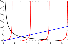
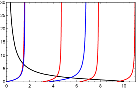
Figure 1: The graphical presentation of the even solutions of (93) for fixed $\gamma=10$ and $a/\lambda$ varying from $1,5,10,20$ from left upper corner till right lower one. The intersections of the black line with blue lines indicate the even solutions to the eigenvalue problem. The red lines indicate the undeformed case with $\lambda=0$.

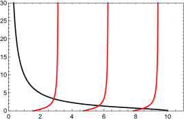
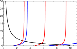
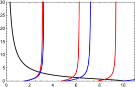
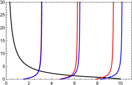
Figure 2: Same as figure 1 but for the odd solutions of (93) with same set of parameters. The case $a=\lambda$ in the left upper graph does not exhibit an odd eigenstate as discussed the text.

It appears that there always exists a ground state. No excited states occur when $\gamma<\frac{a}{\lambda}\tan(\frac{\lambda}{a}\pi)$. In figure 1 and 2 we present graphical solutions for both conditions (93) for fixed value $\gamma=10$ and $a/\lambda=1,5,10,20$, respectively. Figure 1 shows the even solutions related to the first condition in (93). The black line presents the left-hand-side of this condition, whereas the blue lines show the right-hand-side of (93). In addition, we added red lines indicating the undeformed case, see the leading term below in eq. (94). The parameter $a/\lambda$ varies from $a/\lambda=1$ in the left upper graph to $a/\lambda=20$ in the right lower one. Figure 2 shows the same graphs but for the odd solutions in (93). Both figures clearly show that with increasing width the GUP potential well accumulates more and more bound states, indicated by the intersections of the black and blue lines. For increasing $a$ the difference to the undeformed potential well becomes less invisible, in particular for the lower eigenvalues. For $a=20\lambda$ the ground state energy is essential identical to that of the undeformed case as the red curve completely disappeared underneath the blue one.

For $a\gg\lambda$ one obtains the approximate conditions

$$\frac{\sqrt{\gamma^{2}-y^{2}}}{y}=\left\{\begin{array}[]{ll}\tan y-\frac{1}{3}\frac{\lambda^{2}}{a^{2}}y^{3}\left(1+\tan^{2}y\right)+O(\frac{\lambda^{4}}{a^{4}})&\mbox{for}~{}\phi_{+}\\[5.69054pt] -\cot y-\frac{1}{3}\frac{\lambda^{2}}{a^{2}}y^{3}\left(1+\cot^{2}y\right)+O(\frac{\lambda^{4}}{a^{4}})&\mbox{for}~{}\phi_{-}\end{array}\right.\,.$$ (94)

Clearly $\lambda=0$ reproduces the standard textbook result indicated by the red curves in both figures.

For the special case $a=\lambda$ the above conditions (92) allow for an analytic solution as they are reduced to

$$\kappa=\lambda q^{2}\qquad\mbox{and}\qquad\kappa=-\frac{1}{\lambda}\,.$$ (95)

As $\kappa>0$, we have to discard the second solution belong to an odd eigenstate and we remain with a single bound state with energy eigenvalue given by

$$E_{1}=V_{0}+\frac{1}{4M\lambda^{2}}\left(\sqrt{1-8V_{0}M\lambda^{2}}-1\right)\,.$$ (96)

Here we observe that for $a=\lambda\to 0$ this approaches the value $E_{1}\to 0$ and the ground state disappears.

To conclude this discussion on the square well, let us look at the limit of small $a$ and large $V_{0}$ such that the product $\alpha:=a|V_{0}|$ remains constant. That is, in the limit $a\to 0$ the box simulates a $\delta$ potential. For small $a$ relation (89) results in a large $q$ approximately given by $q^{2}\approx\frac{2M\alpha}{a}$. For large $q$ a little exercise shows that $\tan(\varphi(q)a)\approx\frac{\pi}{2}\frac{a}{\lambda}$. Hence, via eq.  (92) we arrive at the ground state energy

$$E_{1}\approx-\frac{a\alpha\pi^{2}}{4\lambda^{2}}\,.$$

That is, in the limit $a\to 0$, which simulates a potential $V(x)\to 2\alpha\delta(x)$, the ground state disappears again. In other words, the Dirac $\delta$-potential does not have a bound state in gravitational quantum mechanics. For that reason we will consider a GUP deformed $\delta$ potential as final example.

The GUP delta potential problem:
Our last potential to be considered in the current framework is the attractive GUP $\delta$-function potential,

$$V(x):=-\alpha\,\delta_{\varphi}(x)\,,\qquad\alpha>0\,.$$ (97)

We are only interested in a possible bound state and set $E=-\kappa^{2}/2M$ resulting in the Schrödinger equation

$$\left(D_{x}^{2}-\kappa^{2}\right)\psi(x)=2M\alpha\delta_{\varphi}(x)\psi(x)$$ (98)

Obviously, the normalised solution reads

$$\psi(x)=\sqrt{\frac{{\rm arctanh}(\lambda\kappa)}{\lambda}}\,e_{\beta}(-\kappa;|x|)=\sqrt{\frac{{\rm arctanh}(\lambda\kappa)}{\lambda}}\,{\rm e}^{{\rm i}\varphi({\rm i}\kappa)|x|}=\sqrt{\frac{{\rm arctanh}(\lambda\kappa)}{\lambda}}\,{\rm e}^{-{\rm arctanh}(\lambda\kappa)|x|/\lambda}$$ (99)

and its width is given by

$$\Delta x=\frac{\lambda}{2{\rm arctanh}(\lambda\kappa)}=\frac{1}{2\kappa}\left(1-\frac{\beta}{3\kappa^{2}}+O(\beta^{2})\right)\,.$$ (100)

In order to obtain the allowed value for $\kappa$ let us GUP-integrate equation (98). That is, we consider

$$\int_{-\varepsilon}^{\varepsilon}{\rm D}_{\varphi}x\,\left(D_{x}^{2}-\kappa^{2}\right)\psi(x)=2M\alpha\int_{-\varepsilon}^{\varepsilon}{\rm D}_{\varphi}x\,\delta_{\varphi}(x)\psi(x)=2M\alpha\psi(0)$$ (101)

The integral on the left-hand-side is easily integrated with the help of (30) and results in $2\kappa\psi(0)$ in the limit $\varepsilon\to 0$. This way we identify $\kappa=M\alpha$. That is the energy of the state bounded by the GUP delta potential is given by

$$E=-\frac{M\alpha^{2}}{2}$$ (102)

and coincides with the result of undeformed quantum mechanics for the attractive Dirac-delta potential. The difference to ordinary quantum mechanics is in the deformed eigenfunction.

7 Summary

In this paper we have presented an algebraic approach to gravitational quantum mechanics being based on a deformed Heisenberg algebra resulting in a generalized uncertainty principle. The GUP introduces a minimal length $\lambda$ being directly related to the deformation parameter $\beta=\lambda^{2}$, and has severe effects on the associated quantum models. For the investigation of such deformed quantum mechanical models, we were inspired by the non-Newtownian or $g$ calculus and introduced a GUP calculus well adopted to the underlying structure. This is an essential ingredient to obtain exact solutions for several models in gravitational quantum mechanics.

The plane-wave solutions where shown to be characterised by the so-called GUP exponential function which allowed a superposition to form a Gaussian wave packet. It appears that details of such wave packets are lost when decomposing them into their plane wave components. However, such details are shown to be exponentially small and hence, can be ignored when looking into effects being of the order of $\beta$. This has let us to introduce the GUP Fourier transformation, which is an approximation of the standard Fourier transformation. This enabled us to look into the time evolution of a Gaussian wave packet, which was analysed to first order in $\beta=\lambda^{2}$. The corresponding uncertainty relation has been present explicitly to second order in time.

We further investigated several models where the GUP particle interacts with an external potential, for which we could solve exactly the corresponding eigenvalue problem with the help of the GUP calculus. For the particle enclosed in a box it turned out that the corresponding energy eigenfunction are identical in form with those of the undeformed case. The effect of a minimal length only shows up in the corresponding spectrum which consists of a finite number of eigenvalues only. This is clearly due to the effect of a minimal length as for a box of size $L<2\lambda$ no energy eigenstates exist at all as they would require an infinite amount of energy.

The situation is different when considering a potential well with a finite depth $-V_{0}$ and a width of size $2a$. Here again only a finite number of bound states exits but for any $a>0$ there at least is one bound state. For large $a\gg\lambda$ the low-lying eigenvalues are very close to those of the undeformed case. For the special case $a=\lambda$ only one bound state exists whose eigenvalue could be given in closed form. The particular case where $a\to 0$ and $V_{0}\to-\infty$ such that $a|V_{0}|$ remains constant the well simulates a Dirac delta potential but does not have any bound state in that limit.

This has let us to the last example where the particle is interacting with an attractive GUP delta potential. This function was introduced in our GUP calculus and is a deformed version of Dirac’s delta function. It was found that this potential generates precisely one bound state whose energy eigenvalue is identical in form with that of the undeformed Schrödinger Hamiltonian with the attractive Dirac delta-function potential. The difference to the undeformed quantum model is only visible in the corresponding eigenfunctions.

Appendix: Approximate completeness of GUP momentum eigenfunctions

Let us reconsider the relation (44) which reads

$$\int_{-\infty}^{\infty}{\rm d}P\,u^{*}_{P}(x)u_{P}(x^{\prime})=\int_{-\infty}^{\infty}{\rm d}P\,\frac{{\rm e}^{{\rm i}\varphi(P)(x-x^{\prime})}}{2\pi(1+\beta P^{2})}\,$$ (103)

Noting that $\varphi(P)=P-(\beta/3)P^{3}+O(\beta^{2})$ we realise that the $P^{3}$-term in the exponent contributes only with a leading order in $\beta^{2}$ to (103) due to its anti-symmetry. Hence the leading term in $\beta$ comes from the measure $(1+\beta P^{2})^{-1}=1-\beta P^{2}+O(\beta^{2})$. This brings us to the approximate completeness relation

$$\begin{array}[]{rl}\displaystyle\int_{-\infty}^{\infty}{\rm d}P\,u^{*}_{P}(x)u_{P}(x^{\prime})&\displaystyle=\frac{1}{2\pi}\int_{-\infty}^{\infty}{\rm d}P\,{\rm e}^{{\rm i}P(x-x^{\prime})}\left(1-\beta P^{2}+O(\beta^{2})\right)\\[11.38109pt] &\displaystyle=\delta(x-x^{\prime})+\beta\delta^{\prime\prime}(x-x^{\prime})+O(\beta^{2}).\end{array}$$ (104)

That is, the first order correction term in $\beta$ is represented by a second-order derivative of the delta function.

Declarations

The authors did not receive support from any organization for the submitted work.
The authors have no conflicts of interest to declare that are relevant to the content of this article.

References

• [1] Matvei Bronstein, Quantentheorie Schwacher Gravitationsfelder, Physikalische Zeitschrift der Sowjetunion 9 (1936) 140–157. doi:10.34663/9783945561317-22
• [2] Hartland S. Snyder, Quantized space-time, Physical Review 71 (1947) 38-41. doi:10.1103/PhysRev.71.38
• [3] Sabine Hossenfelder, Minimal Length Scale Scenarios for Quantum Gravity, Living Rev. Relativity 16 (2013) 2 (90pp). doi:10.12942/lrr-2013-2
• [4] Abdel Nasser Tawfik and Abdel Magied Diab, A review of the generalized uncertainty principle, Rep. Prog. Phys. 78 (2015) 126001 (28pp). doi:10.1088/0034-4885/78/12/126001
• [5] Michael Grossman and Robert Katz, Non-Newtonian Calculus, (Pigeon Cove, Mass., Lee Press, 1972).
• [6] Endre Pap, g-Calculus, Novi Sad Journal of Mathematics 23 (1993) 145-156.
• [7] Marek Czachor, Non-Newtonian Mathematics Instead of Non-Newtonian Physics: Dark Matter and Dark Energy from a Mismatch of Arithmetics, Found. Sci. 26 (2021) 75–95. doi:10.1007/s10699-020-09687-9
• [8] Achim Kempf, Mangano Gianpiero and Robert B. Mann, Hilbert space representation of the minimal length uncertainty relation, Phys. Rev. D 52 (1995) 1108-1118. doi:10.1103/PhysRevD.52.1108
• [9] K. Nozari and T. Azizi, Some aspects of gravitational quantum mechanics, Gen. Relativ. Gravit. 38 (2006) 735–742. doi:10.1007/s10714-006-0262-9
• [10] Pouria Pedram, A higher order GUP with minimal length uncertainty and maximal momentum II: Applications, Physics Letters B 718 (2012) 638–645. doi:10.1016/j.physletb.2012.07.005