Bound-state confinement after trap-expansion dynamics in integrable systems
Abstract
Integrable systems possess stable families of quasiparticles, which are composite objects (bound states) of elementary excitations. Motivated by recent quantum computer experiments, we investigate bound-state transport in the spin- anisotropic Heisenberg chain ( chain). Specifically, we consider the sudden vacuum expansion of a finite region prepared in a non-equilibrium state. In the hydrodynamic regime, if interactions are strong enough, bound states remain confined in the initial region. Bound-state confinement persists until the density of unbound excitations remains finite in the bulk of . Since region is finite, at asymptotically long times bound states are “liberated” after the “evaporation” of all the unbound excitations. Fingerprints of confinement are visible in the space-time profiles of local spin-projection operators. To be specific, here we focus on the expansion of the -Néel states, which are obtained by repetition of a unit cell with up spins followed by down spins. Upon increasing , the bound-state content is enhanced. In the limit one obtains the domain-wall initial state. We show that for , only bound states with are confined at large chain anisotropy. For , also bound states with are confined, consistent with the absence of transport in the limit . The scenario of bound-state confinement leads to a hierarchy of timescales at which bound states of different sizes are liberated, which is also reflected in the dynamics of the von Neumann entropy.
1 Introduction
Integrable quantum many-body systems provide an ideal playground to discover exotic behaviors both at equilibrium and out-of-equilibrium. As recognized already by Bethe [1], one of the hallmarks of interacting many-body systems is the formation of multiparticle bound states. In spin chains they are formed by elementary magnon-like excitations. Bound states play a pivotal role in the equilibrium and out-of-equilibrium integrable systems, as they enter prominently in the Thermodynamic Bethe Ansatz [2] approach. Since the birth of Bethe Ansatz, bound states attracted growing attention, also experimentally [3, 4, 5, 6, 7, 8]. Furthermore, bound states are key ingredients behind exotic transport behaviors, such as superdiffusion [9]. Very recently, they have been observed in quantum-computing platforms [10].
Here we investigate the dynamics of bound states after trap-expansion experiments in the Heisenberg spin chain, which is a prototypical integrable system [2]. Our out-of-equilibrium protocol is depicted in Fig. 1: A region of size is embedded in an infinite chain, and is prepared in a product state. The rest of the chain is in the ferromagnetic state with all the spins down. The ferromagnetic state is the vacuum state for the Bethe Ansatz quasiparticles. The full chain then evolves under the Hamiltonian. Crucially, the chain, for anisotropy possesses bound states of an arbitrary number of elementary excitations. During the dynamics, as the state of region is not an eigenstate of the model, region undergoes a nontrivial evolution, whereas the remaining part of the chain does not evolve because the ferromagnetic state is eigenstate of the Hamiltonian. The dynamics of region is understood in terms of the thermodynamic excitations [2] of the model. In the limit , at long times local observables in the bulk of region are described by a thermodynamic macrostate, which is a Generalized Gibbs Ensemble [11] (). The initial inhomogeneity that is present at the interface between region and the rest (see Fig. 1) “melts” during the dynamics. This is due to excitations leaving region , where they are initially produced. At long times and large distances from the interface, the state of the system is described by a space-time dependent , which can be obtained within the Generalized Hydrodynamics () approach [12, 13]. In contrast with free-fermion systems, the thermodynamic excitations of the chain are interacting. However, only elastic scattering is allowed, due to integrability. During the scattering the identity of the quasiparticles is preserved. The net effect of the scatterings is to dress the “bare” velocities of the quasiparticles. The dressed velocities depend on the space-time density of quasiparticles, and hence on the initial state. Crucially, the dressing can be so dramatic that the sign of the velocities change. Typically, this is more striking for the bound states, because their bare velocities (see section 5) are typically smaller than the magnons, implying that the bound states are more affected by scatterings. As we will show, this leads to bound-state confinement, meaning that the bound states remain trapped in region where they are produced (see Fig. 1). This was observed already in Ref. [14] (see also [15]). Moreover, the sign change of the bound-state velocities was analyzed at the level of the space-time trajectories in Ref. [16], and it has striking effects on the entanglement dynamics [16, 17]. Besides confinement, the presence of bound states gives rise to several intriguing transport behaviors, such as nonanaliticities in the profile of local observables [18].
Here by combining the time-dependent Density Matrix Renormalization Group [19] () with state-of-the-art integrability methods [20, 21], we provide a thorough investigation of bound-state confinement in the chain at anisotropy . We show that for generic initial states of region , multiparticle bound states remain confined in . Precisely, this happens provided that interactions, i.e., the anisotropy , are strong enough, and there is a finite density of magnon-like quasiparticles, i.e., unbound ones, in region . Confinement is present at large , and it can be understood perturbatively in the limit . Upon lowering there is a threshold below which the lighter bound states, i.e., formed by two elementary quasiparticles, are not confined. This means that two-particle bound states are allowed to leave region (see Fig. 1). This is in agreement with the results of Ref. [14] and [15] for the case of Néel and Majumdar-Ghosh initial states. Moreover, for typical initial states of region there is a hierarchical emission of bound states, meaning that heavier bound states are “liberated” at lower . While confinement can be understood perturbatively, the de-confinement happens near , i.e., away from the perturbative regime. This means that the deconfinement pattern of the different bound states depends on the details of the initial state. Finally, it is important to stress that bound-state confinement happens at ballistic level, i.e., in the hydrodynamic limit with , with the distance from the interface between and (see Fig. 1).
Crucially, since the size of (see Fig. 1) is finite, at long times the density of magnon quasiparticles in vanishes. In turn, this implies that after the “evaporation” of all the magnons from region , the system cannot support bound-state confinement. Thus, even for large bound states cannot remain confined at arbitrarily long times (see Fig. 1 (c)) if region is finite. Still, the short-time behavior of the spin projectors on consecutive sites are reminiscent of confinement. Following Ref. [22], we use as witness for -particles bound-states. We observe that if interactions are not strong enough to support confinement in the hydrodynamic limit, at short times the projectors exhibit a “halo” signal around the interface between and its complement. On the other hand, if confinement is present, the projectors exhibit a “bottleneck” at the interface between and before the “deconfinement” of the bound states happens at longer times.
Finally, we confirm the confinement scenario by considering a “cut” quench (see Fig. 1 (b)) in which the expansion is stopped after a time . The stopping time is chosen such that the density of magnons in is finite, i.e., before the bound-state deconfinement starts. For only part of the chain is further evolved. If interactions are strong enough to permit bound-state confinement, the projectors do not show any signal at in region .
In this work we focus on the vacuum expansion of the -Néel states, which are “fattened” version of the Néel state. They are defined by repetition of a unit cell containing up spins followed by down spins (see Fig. 1 (a)). In the limit the -Néel states converge to the domain-wall state. Interestingly, for transport is suppressed after the quench from the domain-wall state [23]. At transport is neither ballistic nor diffusive, but a superdiffusive dynamics is expected [24]. An interesting feature of the -Néel state is that by changing , one can change the bound-state content. Precisely, states with larger contain more bound states. For one recovers the standard Néel state, which is somewhat special because for the describing the bulk of can be determined analytically [25]. This is not the case for [26], although the can be obtained at modest numerical cost by using the results of Ref. [20]. If region (see Fig. 1) is prepared in the Néel state (with ), at large enough , bound states are confined, as observed in Ref. [15]. Interestingly, for , only bound states with size are confined, whereas for bound states of size are also confined. Since bound states with dominate the behavior of local observables after the quench from the -Néel states, this is compatible with the absence of transport in the limit.
Finally, we show that bound-state confinement has striking consequences on the dynamics of entanglement entropy. First, within the quasiparticle picture for entanglement dynamics [27, 28, 29], entanglement is created in region . Transport between and the rest does not generate new entanglement, but entanglement is simply “transported” from to the rest [17]. We focus on the full expansion of the Néel state. We numerically show that the hierarchical emission of bound states of different sizes is reflected in a multistage growth of the entanglement entropy.
The manuscript is organized as follows. In section 2 we introduce the spin chain and the out-of-equilibrium protocols. In section 3 we review the Thermodynamic Bethe Ansatz of the model. In section 4 we discuss the Generalized Hydrodynamics () approach. In section 5 by using the approach, we investigate bound-state confinement. In particular, in section 5.1 we provide numerical results confirming bound-state confinement after the expansion of the -Néel states. In section 6, we discuss numerical results for the trap-expansion dynamics. In particular, in section 6.1 we discuss the validity of the approach. In section 6.2 and section 6.3 we provide data for the full-expansion dynamics and the cut protocol (see Fig. 1 (a) and (b)), respectively. In section 7, we focus on the entanglement entropy after the full-expansion protocol. We conclude and discuss future directions in section 8.
2 Model and quantum transport protocols
Here we focus on the spin- anisotropic Heisenberg chain ( chain) defined by the Hamiltonian
| (1) |
where are Pauli matrices, is the co-called anisotropy parameter, and is the length of the chain. We focus on the situation with . We employ periodic boundary conditions. However, since our results do not depend on boundary conditions we employ open boundary conditions in the numerical simulations [19]. For both periodic and open boundary condition, the is integrable by the Bethe Ansatz [2].
Here we consider the expansion of “fat” Néel states (see Fig. 1 (a)). They are obtained by repetition of a unit cell containing spins, with spins being up and down. We denote these -Néel states as . The generic -Néel state reads as
| (2) |
where denotes the tensor product.
The quench protocols that we employ are described in Fig. 1 and . In both and the initial state at is obtained by embedding a chain of size prepared in the state in the vacuum state, i.e., the ferromagnetic state with all the spins down . Importantly, since is an eigenstate of (1) for any , only region (see Fig. 1) exhibits a nontrivial dynamics.
In protocol the full system undergoes unitary dynamics under the Hamiltonian (1). In the second protocol (Fig. 1 ) we evolve the full system up to a time . As the dynamics progresses, the initial -Néel state “melts”. For the evolution happens under the Hamiltonian (1) restricted to the region on the right of (see Fig. 1), whereas part of the system is “frozen”. We choose large enough to ensure that the system is in the hydrodynamic limit but not too large, so that region contains a finite density of unbound particles. As we will discuss in section 5, the latter condition is crucial to observe bound-state confinement.
As anticipated, in both protocols and of Fig. 1, at part of the chain “melts” because is not an eigenstate of (1). First, the dynamics of an infinite homogeneous chain prepared in gives rise to a Generalized Gibbs Ensemble [11] () with extensive thermodynamic entropy. Provided that is large enough, local properties in the bulk of region are described by the arising in the homogeneous chain. Oppositely, at the interface between region and the rest, the dynamics leads to the formation of a nontrivial profile. Specifically, in the long-time limit, provided that , to ensure that the central region has a finite density of excitations, ballistic transport sets in. This means that expectation values of generic local observables (with measured from the interface between and rest) are functions of , and not of space and time separately. The expectation values of can be obtained (see section 4) by using the Generalized Hydrodynamics [13, 12] (). Crucially, since the chain is interacting, for sufficiently large transport of bound states (of arbitrary size) of elementary excitations from region to is inhibited in the ballistic regime. This means that the expectation values for are fully determined by magnon-like excitations. This bound-state confinement happens for both the protocols of Fig. 1. As already stressed, for the protocol in Fig. 1 the dynamics at asymptotically long times leads to zero density of magnon-like excitations in the bulk of . As we will discuss in section 5 this will lead to the deconfinement of bound states.
3 Thermodynamic Bethe Ansatz () for quenches from homogeneous states in the chain
To derive bound-state confinement after the trap expansion of the -Néel states (cf. (2)), it is necessary to construct the describing the steady state after the quench from the homogeneous -Néel states. Here we provide a self-contained discussion of the derivation of the for a generic pre-quench initial state. We follow Ref. [20, 21].
We employ the framework of the Thermodynamic Bethe Ansatz [2] (). The eigenstates of the chain are identified by a set of complex numbers , which are called rapidities. Each eigenstate is written as , and the rapidities label the different quasiparticles in the system. In the thermodynamic limit at fixed density of quasiparticles, it is convenient to work with the rapidity density. Moreover, in the thermodynamic limit generic integrable systems exhibit different families of quasiparticles. They correspond to bound states of elementary, magnon-like, excitations. The corresponding rapidities form string patterns in the complex plane [1]. Then, any thermodynamic macrostate of the system is characterized by a set of rapidity densities , where the number of families depends on the model under consideration. For the chain at one has , meaning that bound states of arbitrary sized are present. Similar to the densities , one defines the hole densities . The particle and hole densities for any legitimate macrostate satisfy the equation [2] as
| (3) |
where is the total density. The symbol in (3) denotes the convolution, i.e.,
| (4) |
| (5) |
where the parameter is related to the anisotropy as
| (6) |
Moreover, the parameters in (3) are obtained as
| (7) |
where is defined in (5). Here is related to the scattering phase between a -particle and a -particle bound state as . For the following, it is useful to notice that the “bare” velocities of the quasiparticles are given as
| (8) |
where the energy and the quasimomentum are defined as
| (9) |
Notice that Eq. (3) allows to obtain only one of the densities, either or . Crucially, to uniquely identify a thermodynamic macrostate, one has to determine both the particle and the hole densities. In the following, instead of and we will often consider the ratios and defined as
| (10) |
We now show that the information about the expectation values of local and quasilocal conserved quantities over the pre-quench initial state allows to fix uniquely the densities identifying the that describes the steady state after the quench.
A central object in the Algebraic Bethe Ansatz treatment [30] of the chain is the spin- Lax operator defined as
| (11) |
where is defined in (6) and is a real parameter. For , which corresponds to spin- representation, one has , with . Moreover, are the standard combinations , with Pauli matrices. The Lax operator acts as a matrix over the physical Hilbert space of the model. The entries of (11) live in the “auxiliary” Hilbert space of dimension . Thus, the global Hilbert space is . The auxiliary space is spanned by vectors with , with being a highest-weight vector. The operators with are -deformed spin- operators, forming the -representation of the -deformed algebra . They obey the commutation relations
| (12) |
The action of the operators on the states is given as
| (13) | |||
| (14) | |||
| (15) |
Thus, the eigenvalues of are .
As usual in Algebraic Bethe Ansatz [30], one can construct a set of conserved quantities from the transfer matrix , which is defined as
| (16) |
where the trace is over the auxiliary space. In (16) the superscript in is to stress that it acts in the space , where is the spin- Hilbert space of site of the chain. Moreover, in (16), is given as
| (17) |
A complete set of local and quasilocal conserved charges , which commute with , is defined as [21]
| (18) |
where we introduced the notation
| (19) |
for a generic operator , and is defined in (16). The transfer matrices satisfy the commutation relations
| (20) |
One can also check that the transfer matrices in (22) satisfy a Hirota equation (or the so-called -system) as [21]
| (21) |
Importantly, one can also verify the - relation as [31]
| (22) |
where is the so-called Baxter -operator. The spectrum of the operator is given as , with solutions of the Bethe equations. Crucially, the operator commutes with the transfer matrices , and it can be used to construct a solution of the Hirota equations (21) (see Ref. [20]). In particular, by expanding the solution of (21) in terms of the operator, it has been shown that in the thermodynamic limit one has that [21]
| (23) |
where we defined the scattering matrix between a magnon and a -particle bound state, and is the number of -particle bound states in the Bethe state. Importantly, we can now employ Eq. (23) to compute the expectation value of the local and quasilocal conserved quantities (cf. (18)). Specifically, from (18) and (23) we obtain
| (24) |
where is defined in (23). Notice also that is defined in (7). Following the standard approach [2], in the thermodynamic limit we can replace the sum over the rapidities with an integral weighted with the root density as
| (25) |
where the symbol denotes convolution (cf. (4)). Crucially, it can be shown that [20] the kernel is the Green’s function for the discrete Laplacian operator , which acts on a generic function as
| (26) |
where is a Dirac delta. Now, we can invert (25) by applying the Laplacian on both sides, to obtain
| (27) |
where is defined in (26). Eq. (27) states that one can obtain the densities describing a thermodynamic macrostate (such as the arising after a quench) starting from the expectation values of the quasilocal charges . By using the equation (3), one can obtain the analog of (27) for the hole densities as
| (28) |
where we employ the definition in (19), is the expectation value of the generic quasilocal conserved quantity on the initial state, and is the same as in (5).
To proceed, one has to determine the expectation value of both members of (18) over the initial state . A major complication is that Eq. (18) requires the inverse of the transfer matrix , which is a daunting task in general. Fortunately, in the large limit one can show that [21]
| (29) |
Eq. (29) provides an inversion formula. This is crucial to rewrite the logarithmic derivative in (18) as
| (30) |
which holds in the large limit.
We are now ready to compute the expectation value of over the initial state . Here we consider initial states that are obtained by repeating a unit cell of length , as it is the case for the -Néel states (2). This allows us to rewrite (30) as
| (31) |
where we denoted with the expectation value of the charges over the initial state, and with the unit cell that is used to build . In (31) the Lax operators are obtained from the original ones in (11) by using (19), and the trace is over the auxiliary Hilbert space. Notice that the expectation value over the state of the unit cell involves the physical Hilbert space. Finally, in (31) we shifted the argument of the second term in the brackets to bring the derivative outside of the expectation value. Eq. (31), together with Eq. (27) and Eq. (28), is the main tool to determine the . It is useful to observe that Eq. (31) can be rewritten as
| (32) |
where we defined as
| (33) |
with
| (34) |
4 Generalized Hydrodynamics () for quenches from inhomogeneous initial states
Here we introduce the framework of Generalized Hydrodynamics [13, 12] () to describe the expansion dynamics (see Fig. 1). This will allow us to characterize the bound-state confinement in section 5.
In the standard setup two semi-infinite homogeneous but different initial states are joined together at at the origin . At the full system evolves under a homogeneous integrable Hamiltonian. For typical initial states, at long times and large distances with the ratio fixed, the behavior of the system is described by a -dependent . This is fully characterized by a set of densities and . The densities satisfy the equations (3) for any and the equation, which reads as [12, 13, 17]
| (35) |
Here are the filling functions (cf. (36)) defined as
| (36) |
with the total density. In (35), are the dressed velocities, which are defined as
| (37) |
where and are respectively the bare energy and quasimomentum of the quasiparticles, defined in (9). Given a generic “bare” quantity , its dressed version is obtained by solving the integral equation as [32, 30]
| (38) |
where is defined in (7), and the filling function is given in (36). It is clear from the definition of the momentum as [2]
| (39) |
that the dressing of is obtained by considering in (38).
To solve (35) one has to provide the boundary conditions at . Let us consider the prototypical setup in which the initial state is obtained by joining two semi-infinite chains prepared in two macroscopically different states. This is the so-called bipartite quench protocol [17]. Let us denote by and the two thermodynamic macrostates, i.e., the filling functions, describing the steady state arising at infinite time after the quench from the left and right homogeneous states. The functions , provide the boundary conditions in (35). Before proceeding, one can observe that Eq. (35) can be solved for each separately. It is straightforward to check that the solution of (35) can be written as
| (40) |
where is the Heaviside step function. The dressed velocity in (40) is obtained by using (38) and (37) (39). Notice that since depends on via (38), Eq. (40) is not an explicit solution of (35). To obtain one can use an iterative strategy, starting from (40) fixing , with the “bare” velocities (cf. (8)). Then, one substitutes Eq. (40) in (38) to obtain the dressed . By using the equation (3) one obtains and the new dressed velocities via (37). Finally, these steps are iterated until convergence.
Notice that although the setup of the bipartite quench is different from the one described in Fig. 1 (a), the two protocols give the same dynamics provided that (see Fig. 1) is large enough to ensure that the bulk of region is in the hydrodynamic limit and is large, but short enough to neglect the fact that region is finite. Here is the maximum velocity in the system, i.e, .
In the following we focus on the macrostate with , which describes the interface between the two chains. We also consider the situation in which the right chain is prepared in the vacuum state (see Fig. 1). This corresponds to for any . Now, Eq. (40) becomes
| (41) |
In the following we neglect the subscript in and since we always consider .
5 Bound-state confinement after trap-expansion experiments
Here we discuss the confinement of the bound states for the expansion protocol of Fig. 1 for generic initial state of part (see Fig. 1). The state of corresponds to fixing in (41). Let us summarize our main results. We show that for moderately large ballistic transport of bound states is inhibited, for quite generic initial states of part . Specifically, in the hydrodynamic limit only quasiparticles with , i.e., unbound quasiparticles, can be present at . This means that all the bound states with remain confined within region in Fig. 1 (a).
Bound-state confinement can be understood perturbatively in the large limit, and it relies on the behavior of the scattering phases (7). Indeed, the only assumption on the initial state of region is that it gives rise to macrostates with density of quasiparticles with . Although bound-state confinement is established in the large limit, it survives up to . Precisely, for the Néel state bound state confinement survives up to [15] . Upon lowering below , bound states with start to leave region . For bound states with are not confined. However, while the threshold for confinement of the two-particle bound states is understood perturbatively, this is not the case for the larger bound states. Indeed, the deconfinement of bound states with happens in the nonperturbative regime at , and is sensitive to the details of the initial state. Crucially, since region is finite (see Fig. 1), the condition that the density of quasiparticles with is finite in , which ensures the bound-state confinement, is necessarily violated at long times. This implies that at times excitations with can leave region , i.e., they are not confined anymore.
Bound-state confinement manifests itself in the fact that the dressed velocities at are negative for any and for any . To proceed, let us assume that only bound states with , for some , are confined. This implies that Eq. (38) for becomes
| (42) |
where , and is such that for any and for any . Notice that in (42) we replaced with in the argument of the Heaviside theta function. This is possible because (cf. (37)) is positive. Also, notice that in the integrand in (42) one has that and are both positive functions. For (42) to be consistent with confinement of the bound states with , we require that the solutions of (42) satisfy the condition
| (43) |
Clearly, while the dressing (38) for the with is a system of infinite equations since , the system (42) is finite. Still, given the solutions of (42), one has to check the validity of (43) for any .
Before proceeding, it is interesting to observe that , meaning that not all the species of quasiparticles can be confined at the same time, at least in the hydrodynamic limit. Indeed, implies (cf. (42)) that , and is not negative for all values of (cf. (8)). This implies that the suppression of ballistic transport observed for instance in the domain-wall quench [23] cannot be attributed to the bound-state confinement.
The conditions under which the systems (42) and (43) admit a solution can be derived in the large limit. First, let us observe that for any . Moreover, in the large limit, at the leading order in powers of , one has that for any . Precisely, for large one has that
| (44) |
and otherwise. Finally, it is straightforward to check that the bare velocities (cf. (8)) at the leading order in the large limit are
| (45) |
Here we defined , and for large one has . Moreover, unlike the dressed velocities, the bare ones do not depend on the pre-quench initial state, so (45) holds irrespective of the initial state of (see Fig. 1). Crucially, while the bare velocities of the quasiparticles with are , the bound-state velocities for decay exponentially with the bound-state size . This hierarchy in the bare velocities is responsible for the bound-state confinement.
Let us consider the case with , i.e., the situation in which in region there is a finite density of unbound quasiparticles. This happens for typical states, such as the Néel state and the Majumdar-Ghosh state [15]. We anticipate that the -Néel states with do not satisfy this condition. Let us also assume that , i.e., bound states with remain confined within during the expansion dynamics.
Now, let us consider Eq. (42) with . It is clear that the second term in the right-hand side dominates for large because for , whereas the first term in (42) is . Clearly, the same argument applies also for , implying that all the bound states with are confined for sufficiently large . Interestingly, as the only dependence on in the second term in (42) is in , which becomes independent of for large , the dressed velocities of the confined bound states become “flat” as functions of .
Upon lowering , the two terms in (42) become of the same order, and quasiparticles with start to be transported in (see Fig. 1). Notice that while bound-state confinement can be established perturbatively, and even the threshold at which bound states with are not confined can be calculated from the large expansion, it is difficult to characterize analytically the scenario for . Typically, we observe that there is a “cascade” effect. Precisely, upon lowering , transport of bound states with progressively larger become allowed (see section 5.1).
The scenario outlined so far relies on the fact that at any time during the expansion . This condition remains true at arbitrarily long times if region (cf. Fig. 1) is infinite. Oppositely, if region is finite, at long times one has that vanishes. This implies that the second term in (42) becomes smaller. Thus, at long times the bound states with can leave region after the “evaporation” of the unbound particles. Moreover, the condition is not valid for generic initial states. For instance, it is violated by all the -Néel states with generic . By using the framework of section 3, one can check that for , whereas for . This has striking consequences on transport properties and bound-state confinement. Indeed, we anticipate that the fact that implies a strong suppression of bound-state transport for . Let us first consider the case with . Now, Eq. (42) suggests that bound states with are not confined. Indeed, the term with in the right-hand-side of (42) is and it is negligible compared to . This means that unlike the case with the two-particle bound states cannot be confined by the magnons. Now, if we consider the case with we observe that since , it is clear that the second term in (42) dominates because of the scatterings with the quasiparticles with , which contribute with terms with smaller powers of . This implies that upon increasing the bound states that dominate the thermodynamic properties, i.e., the bound states with , become confined, and transport is suppressed.
5.1 Bound-state confinement: Numerical GHD results
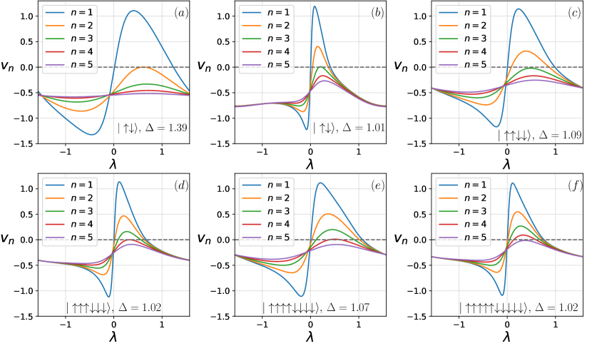
Although qualitative features of bound-state confinement are understood perturbatively, to characterize quantitatively bound-state confinement it is necessary to determine numerically the dressed velocities . Here we discuss numerical results confirming the scenario outlined in section 5. Precisely, we numerically solve the equation (35) to obtain the dressed velocities for . The numerical solution of (35) is standard. By using a Gauss discretization, Eq. (35) becomes an infinite system of nonlinear equations, which can be truncated considering only bound states of size . Finally, the truncated system can be solved with standard methods. Here we consider .
Our results are reported in Fig. 2. We plot for versus . We consider as initial states the -Néel states (cf. (2)) with . For the quench is the popular Néel quench. At large one has that for any and for any , meaning that all the bound states are confined within region . Fig. 2 (a) shows that for the faster bound states with start to be transmitted [15]. Upon lowering , at , the bound states with are not confined, as shown in Fig. 2 (b). For , as anticipated in section 5, the bound states with are not confined. We checked the absence of confinement up to , although we do not report the results in Fig. 2. On the other hand, Fig. 2 (c) shows that for at the three-particle bound states are still confined in . A similar scenario occurs for , i.e., the bound states with are not confined, whereas the bound states with are all confined up to . However, the scenario changes at . As it is clear from Fig. 2 (e), for the group velocities are negative for any . This holds true for as well (see Fig. 2 (f)). Since the thermodynamic properties of the system are dominated by the bound states with , this means that transport becomes more and more suppressed upon increasing .
6 Numerical tDMRG results
Here we discuss data [19] for the vacuum expansion protocols introduced in Fig. 1. Our results support the bound-state confinement scenario outlined in section 5. As a preliminary check, in section 6.1 we discuss data for full-expansion protocol in Fig. 1, considering times , such that the fact that region is of finite size can be neglected. We benchmark the results of section 4 for several -Néel initial states. In section 6.2 we focus on the confinement of bound states for the full-expansion protocol (see Fig. 1 (a)). In section 6.3 we discuss the cut quench protocol (see Fig. 1 (b)).
6.1 Validity of GHD
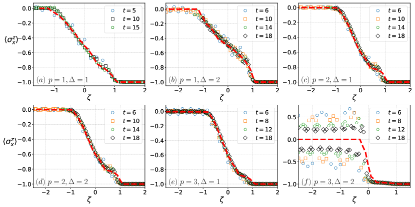
Before investigating bound-state confinement, it is crucial to assess the validity of the description for the protocols discussed in Fig. 1. This is summarized in Fig. 3. We consider the expansion of the -Néel states with . The different panels show data for the local magnetization as a function of . For each we show results for . Here is the distance from the right edge of region (see Fig. 1). In our simulations we consider times to avoid effects due to the finite size of . In Fig. 3 we provide data for several times up to (different symbols in the Figure). The data exhibit collapse when plotted as function of , confirming that is large enough to ensure the hydrodynamic limit for all the values of and considered, except for with (see Fig. 3 (f)). For and the evolution in the bulk of region is slower compared to the other cases. Indeed, at , the magnetization profile exhibits strong oscillations, which are reminiscent of the structure of the initial state. In all the panels, the dashed curve are the results obtained by solving numerically the equation (35). The numerical results were obtained by truncating the infinite system of equations (35) keeping only the bound states with . The equation (35) allows to obtain the occupation functions . The numerical results for can be substituted in the equations (3), after using that . Eq. (3) allows one to obtain the quasiparticle densities , which encode information about local observables. For instance, the local magnetization is given as
| (46) |
For all the quenches that we explore in panels (a-e) of Fig. 3 the results are in satisfactory agreement with the data, despite the limitation to times . For the expansion of the -Néel state with and (panel (f) in Fig. 3) deviations from the prediction are large. Also, notice that for one has that , signaling that transport in general is strongly suppressed for .
As anticipated in section 5 for the -Néel state with , the bound states with remain confined in region , as long as the system is in the hydrodynamic limit, and the description is valid. Specifically, this holds for with fixed, with being the distance from the right edge of region (see Fig. 1). Moreover, for the bound-state confinement to happen, the condition has to be satisfied. This is the case for , at least if .
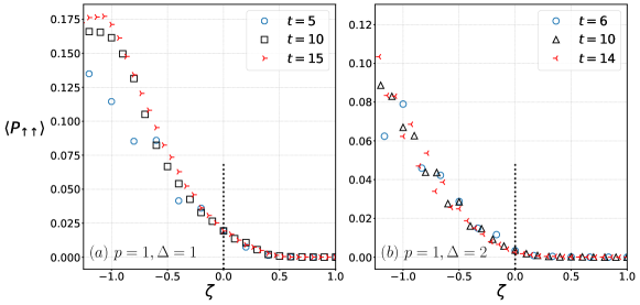
Confinement of the the two-particle bound states is discussed in Fig. 4. The Figure shows (cf. (47)) plotted versus . The projectors are defined as
| (47) |
Although the projectors (47) are not bona fide witnesses of bound states, we anticipate that is sensitive to the presence of a -particle bound state at position . Panels (a) and (b) show data for for the Hamiltonian with and , respectively. In each panel the different symbols correspond to different times. For both and the data exhibit scaling as a function of . Crucially, while for (Fig. 4 (a)) is nonzero for , one has for any for (see Fig. 4). This reflects that while for the bound states with are not confined, for they remain confined in region during the expansion. Still, at , for , which suggests that the density of two-particle bound states that are not confined is “small”, meaning that it could be challenging to observe it, for instance experimentally.
6.2 Full expansion dynamics
In section 6.1 we established the validity of the description for the quenches from the -Néel states. Moreover, Fig. 3 suggests that is enough to access the hydrodynamic limit, which is essential to observe bound-state confinement. We now focus on the full expansion dynamics, i.e., considering times . We show data for the expansion of the -Néel states with for and in Fig. 5 and Fig. 6, respectively. The protocol is reported in Fig. 1. Region at center of the chain is prepared in the Néel state. Here we consider . The reason for choosing is that it allows to simulate the dynamics using up to times . Indeed, entanglement, which is the major limitation of , is produced in the bulk of region only, whereas the expansion does not contribute significantly to the entanglement growth. This also reflects that the dynamics preserves the thermodynamic entropy [14, 16]. As a consequence, the largest entanglement produced during the dynamics is bounded by .
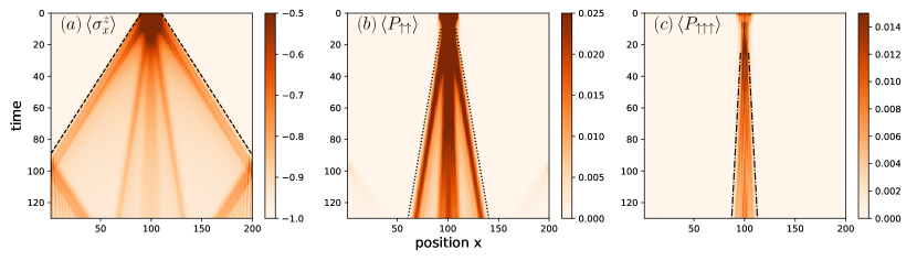
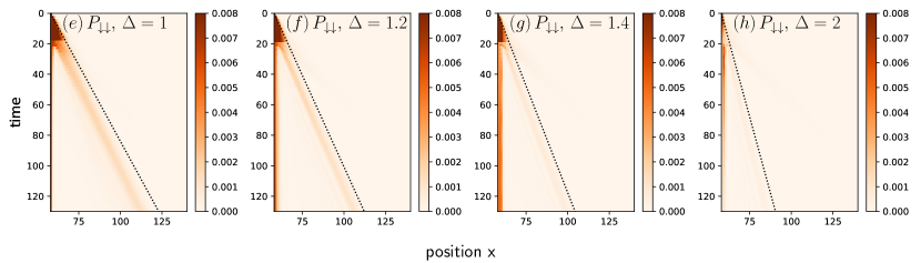
The different panels in Fig. 5 and Fig. 6 show different observables. Precisely, we consider the local magnetization , and the local projectors (cf. (47)). As anticipated, and has already observed in Ref. [22] and Ref. [10], is sensitive to bound states of spins starting from position .
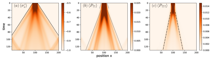
Let us first discuss the dynamics with the chain at (see Fig. 5). In Fig. 5 we plot the density of local magnetization as a function of position and time . After the expansion starts, the central region “melts” as quasiparticles are emitted at its edges. First, several “jets” of excitations are visibile, traveling at different velocities. The fastest quasiparticles correspond to the magnon-like excitations, i.e., with , whereas the jets moving at smaller velocities correspond to bound states with and quasiparticles. The dashed lines are the bare maximum group velocities of the quasiparticles (cf. (8)). Since the initial state is expanded in the vacuum, the density of quasiparticles at the edges of the jets is small and interactions are “weak”, which explains why the bare velocities describe the dynamics of the jets. In Fig. 5 (b) we show the dynamics of the projector . Now, the outermost jet in Fig. 5 (a) is not present, confirming that it is due to the quasiparticles with . Oppositely, the two innermost jets of Fig. 5, corresponding to are still present. Similar behavior was observed in the expansion of few-spin initial states in Ref. [22]. Importantly, one should observe that at short times , exhibits a “halo” feature at the edges of region . This can be attributed to the fact that for the two-particle bound states are not confined in the hydrodynamic limit. Notice, however, that the halo is quite weak, reflecting that the density of two-particle bound states at the interface between and the rest is small. A similar scenario is observed for (see Fig. 5 (c)). Now, the three-particle bound states behave as if they were confined up to . Notice that the fact (see Fig. 2 (b)) that at suggests that the density of three-particle bound states at the interface between and the vacuum could be small. This implies that even though bound states with are not confined at , this could be difficult to observe.
Let us now discuss the same protocol in the chain with (see Fig. 6). The qualitative behavior is the same as in Fig. 5. However, the projector at short times exhibits a “bottleneck” feature. In contrast with , at the two-particle bound states are confined (see Fig. 2 (c)). Moreover, in the hydrodynamic regime the density is zero for , and it is presumably small also at . This explains the bottleneck in Fig. 6 At long times after all the magnons have left region , the two-particle bound states are allowed to leave region , as discussed in section 5, and as it is confirmed in Fig. 6 (b). A similar dynamics happens for the three-particle bound states, as shown in Fig. 6 (c).
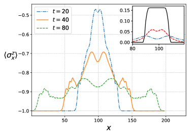
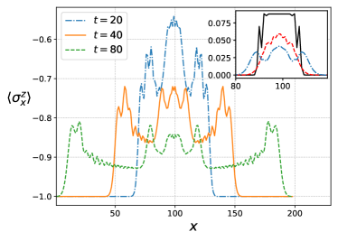
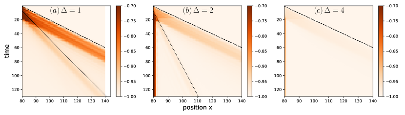
Let us now discuss the space-time profiles of local observables. In Fig. 7 we show the profile of the local magnetization after the expansion of the Néel state for the chain with and , respectively. Both panels in Fig. 7 confirm that for and the bound states with and are not confined at long times, as already observed in Fig. 5 and Fig. 6. The data for (left panel in Fig. 7) show a rapid melting of the profile. As the dynamics proceeds, exhibits a multi-peak structure, each peak corresponding to a different bound-state family. For the peaks are blended together, reflecting that the bound states of different types start to leave region at the same time. In particular, already at the bound states with are moving towards the edges of region . In the inset we show the dynamics of , which is sensitive to quasiparticles with only. The inset shows a rapid melting of . In contrast, for (right panel in Fig. 7) the dynamics is slower, and the peaks corresponding to different are well separated. Notice that at the lump around corresponds to the three-particle bound states, which remain almost locked at the center of the chain. This observation suggests that for the trap-expansion protocol can be used to “distillate” states with large bound-state content. The inset shows the dynamics of . Notice that for the bound states with are still within region . Importantly, for the density of quasiparticles with in the bulk of starts to be small already at , implying that bound-state confinement is not supported anymore (see section 5).
6.3 Dynamics after the cut protocol
To investigate bound-state confinement, it is also convenient to employ the protocol in Fig. 1 (b). The full chain is now evolved with the Hamiltonian up to a time . Here is chosen large enough to ensure the validity of the hydrodynamic limit. As it is clear from section 6.1, is sufficient to ensure the hydrodynamic limit. Moreover, is chosen short enough compared to to have in the bulk of , which is essential to have bound-state confinement. Here we choose and . We consider the -Néel states with .
6.3.1 -Néel state with
Our results for the Néel state (i.e., for ) are shown in Fig. 8. Panels shows the local magnetization , as a function of position and time . As it is clear from the Figure, for (see Fig. 1), under the evolution with the Hamiltonian (1) restricted to the quasiparticles emitted from propagte ballistically in the vacuum. The dependence on is weak. In the bottom row in Fig. 8 (panels (e-h) in the Figure) we report the dynamics of . For , exhibits a ballistic spreading. The nonzero signal reflects that the bound states with are not confined. becomes smaller upon increasing . For instance, it is barely visible at . Notice that in the hydrodynamic limit one should expect that is exactly zero for (see Fig. 2).
6.3.2 -Néel state with
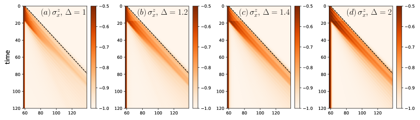
Let us now discuss the cut protocol (see Fig. 1 (b)) for the -Néel state with . Our results are reported in Fig. 9. Panels (a)-(c) show data for the dynamics with the chain Hamiltonian and . In the Figure we plot the local magnetization as a function of position and time . For (Fig. 9 (a)) two distinct signals are visible. The two “jets” correspond to quasiparticles with , i.e., free ones, and to the two-particle bound states. The two-particle jet is due to the fact that for the bound-state content of the chain is enhanced as compared to , and two-particle bound states are not confined at . Notice also that the bound states exhibit smaller group velocities as compared with the quasiparticles with . The dashed lines reported in Fig. 9 (a) are the maximum bare velocities (cf. (8)).
In Fig. 9 (b) we show data for . Crucially, the jet corresponding to the two-particle bound states is still visible. This is in agreement with the results of section 5. Indeed, for one should expect that the quasiparticles with are never confined. On the other hand, as it is clear from Fig. 2 (c), the three-particle bound states are confined for . We should mention that, however, as the density of quasiparticles with is “small”, it is numerically challenging to observe the three-particle bound states confinement. Finally, in Fig. 9 (c) we show results for . Now, the jet corresponding to is weak, in contrast with the case with . This is due to the fact that for the density vanishes, reflecting that thermodynamic properties of the system are dominated by the bound states with . On the other hand, for the maximum group velocity of the two-particle bound states is , and their expansion is barely visible.
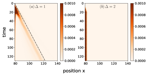
Finally, in Fig. 10 we report the projector after the expansion of the -Néel state with . In Fig. 10 (a) and (b) we show results for and , respectively. While for ballistic spreading is visible, for , the projector is “frozen”.
7 Bound-state confinement and dynamics of the entanglement entropy
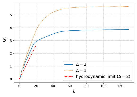
Here we show that bound-state confinement has striking signatures in the dynamics of the von Neumann entropy. We focus on the full expansion of the Néel state (see Fig. 1 (a)). Fig. 11 shows the von Neumann entropy of region (see Fig. 1 (a)). The dotted curve is the result for , whereas the full line shows the result for . First, for both values of the von Neumann entropy saturates at long time. This reflects that the entanglement dynamics is due to the creation of pairs of entangled quasiparticles in region [29]. This is the content of the so-called quasiparticle picture [33, 28, 29, 34]. The two quasiparticles forming the entangled pairs travel with opposite group velocities. As they propagate, they entangle larger regions. Precisely, the von Neumann entropy of a region is proportional to the number of entangled pairs that are shared between the region and the rest. The contribution of a shared pair characterized by rapidities is the contribution of that pair to the thermodynamic entropy of the describing the steady state after the quench from the homogeneous Néel state. The quasiparticle picture holds in the hydrodynamic limit with the ratio fixed.
Let us focus on the results for in Fig. 11. The initial linear growth up to is due to the entangled pairs that are initially produced in and at later times leave region , and hence start to be shared with the rest (see Fig. 1). The saturation of at long times reflects that region is finite, and, as a consequence the number of entangled pairs produced in is finite, and it is proportional to the size of . For , is essentially constant for . The saturation of the entanglement entropy is the key to reach times long as with , because after the entropy saturates the computational cost is mild. One should also observe that the saturation of happens “smoothly”. This is somewhat reminiscent of the fact that for the bound states are not confined. Crucially, for , exhibits a multistage linear growth before saturating. This reflects the bound-state confinement. Specifically, the linear growth up to is due to the quasiparticles with . In this early time regime, the slope of the linear growth should be the same as in the vacuum expansion of a semi-infinite chain prepared in the Néel state. The prediction of the quasiparticle picture is [14, 16]
| (48) |
where is the Yang-Yang entropy [2] of the macrostate with that describes the interface between region and region (see Fig. 1). is readily obtained from the particle densities describing the as
| (49) |
where the densities are defined in section 3 (see also section 4). Notice that in (48) only the quasiparticles with contribute, reflecting that all the bound states are confined in , and cannot contribute to the von Neumann entropy. Now, the data in Fig. 11 exhibit deviations from (48). This is expected because (48) holds in the hydrodynamic limit . Finally, we should mention that it is possible to characterize the trajectories [16] of the the generic entangled pairs produced in , which are responsible of the entanglement growth. This, in principle, could allow to determine also the secondary slopes visible in Fig. 11.
8 Conclusions
We investigated bound-state confinement after trap-expansion experiments in the spin chain at . We showed that after the expansion in the vacuum of quite generic initial states the bound states of the chain remain confined in the initial region, provided that is large enough. Upon lowering the bound states are allowed to leave region , i.e., they are not confined anymore. The condition ensuring confinement is the presence of a finite density of magnon-like excitations in the bulk of the initial region. Physically, bound-state confinement is a genuine consequence of interactions, i.e., the scattering, between the bound states and the magnons. Interestingly, if the size of the initial region is finite, at long times the density of magnons vanishes, as they leave the initial region, and bound-state confinement breaks down. Thus, for the expansion of finite regions, bound-state confinement is present only at intermediate times .
We investigated bound-state confinement after the expansion of the -Néel states (see Fig. 1). In the limit one recovers the domain wall initial state, and transport is suppressed. We showed that for small , bound-state confinement happens for the bound states of size . At larger , even the bound states with are confined, which is consistent with the absence of transport in the limit . Finally, we showed that bound-state confinement is reflected in a multi-stage linear growth of the entanglement entropy.
Let us now discuss some directions for future research. First, we investigated bound-state confinement in a lattice model. It would be interesting to understand whether confinement occurs for systems in the continuum, such as the attractive Lieb-Liniger gas. This would pave the way for the experimental verification of bound-state confinement, for instance with atom-chip experiments [35, 36] or trapped ions experiments [8]. Interestingly, bound-state confinement could be potentially used to prepare thermodynamic states with high bound-state content. Specifically, the protocol to enrich the bound state content would consists of two steps. In a first step one can expand the initial state as in Fig. 1 (a). Then, after the magnon-like excitation are “evaporated” one could trap the remaining excitations by applying an external potential. As the bound states are typically associated with lower thermodynamic entropy, bound-state confinement can also be used to prepare low-entropy states. It has been pointed out recently that bound-states could be robust agains long-range interactions [37, 8]. It would be interesting to understand whether long-range spin chains exhibit bound-state confinement as well. Finally, it would be important to clarify whether bound-state confinement is also present in integrable quantum circuits [38, 39, 40].
Acknowledgements
This study was carried out within the National Centre on HPC, Big Data and Quantum Computing - SPOKE 10 (Quantum Computing) and received funding from the European Union Next-GenerationEU - National Recovery and Resilience Plan (NRRP) – MISSION 4 COMPONENT 2, INVESTMENT N. 1.4 – CUP N. I53C22000690001.
This work has been supported by the project “Artificially devised many-body quantum dynamics in low dimensions - ManyQLowD” funded by the MIUR Progetti di Ricerca
di Rilevante Interesse Nazionale (PRIN) Bando 2022 - grant 2022R35ZBF.
This work has been partially funded by the ERC Starting Grant 101042293 (HEPIQ).
References
References
- [1] Bethe H 1931 Zeitschrift für Physik 71 205–226 ISSN 0044-3328 URL https://doi.org/10.1007/BF01341708
- [2] Takahashi M 1999 Thermodynamics of One-Dimensional Solvable Models (Cambridge University Press)
- [3] Haller E, Gustavsson M, Mark M J, Danzl J G, Hart R, Pupillo G and Nägerl H C 2009 Science 325 1224–1227 (Preprint https://www.science.org/doi/pdf/10.1126/science.1175850) URL https://www.science.org/doi/abs/10.1126/science.1175850
- [4] Fukuhara T, Schauß P, Endres M, Hild S, Cheneau M, Bloch I and Gross C 2013 Nature 502 76–79 ISSN 1476-4687 URL https://doi.org/10.1038/nature12541
- [5] Wang Z, Wu J, Yang W, Bera A K, Kamenskyi D, Islam A T M N, Xu S, Law J M, Lake B, Wu C and Loidl A 2018 Nature 554 219–223 ISSN 1476-4687 URL https://doi.org/10.1038/nature25466
- [6] Bera A K, Wu J, Yang W, Bewley R, Boehm M, Xu J, Bartkowiak M, Prokhnenko O, Klemke B, Islam A T M N, Law J M, Wang Z and Lake B 2020 Nature Physics 16 625–630 ISSN 1745-2481 URL https://doi.org/10.1038/s41567-020-0835-7
- [7] Scheie A, Laurell P, Lake B, Nagler S E, Stone M B, Caux J S and Tennant D A 2022 Nature Communications 13 5796 ISSN 2041-1723 URL https://doi.org/10.1038/s41467-022-33571-8
- [8] Kranzl F, Birnkammer S, Joshi M K, Bastianello A, Blatt R, Knap M and Roos C F 2023 Phys. Rev. X 13(3) 031017 URL https://link.aps.org/doi/10.1103/PhysRevX.13.031017
- [9] Ilievski E, De Nardis J, Gopalakrishnan S, Vasseur R and Ware B 2021 Phys. Rev. X 11(3) 031023 URL https://link.aps.org/doi/10.1103/PhysRevX.11.031023
- [10] Morvan A, Andersen T I, Mi X, Neill C, Petukhov A, Kechedzhi K, Abanin D A, Michailidis A, Acharya R, Arute F, Arya K, Asfaw A, Atalaya J, Bardin J C, Basso J, Bengtsson A, Bortoli G, Bourassa A, Bovaird J, Brill L, Broughton M, Buckley B B, Buell D A, Burger T, Burkett B, Bushnell N, Chen Z, Chiaro B, Collins R, Conner P, Courtney W, Crook A L, Curtin B, Debroy D M, Del Toro Barba A, Demura S, Dunsworth A, Eppens D, Erickson C, Faoro L, Farhi E, Fatemi R, Flores Burgos L, Forati E, Fowler A G, Foxen B, Giang W, Gidney C, Gilboa D, Giustina M, Grajales Dau A, Gross J A, Habegger S, Hamilton M C, Harrigan M P, Harrington S D, Hoffmann M, Hong S, Huang T, Huff A, Huggins W J, Isakov S V, Iveland J, Jeffrey E, Jiang Z, Jones C, Juhas P, Kafri D, Khattar T, Khezri M, Kieferová M, Kim S, Kitaev A Y, Klimov P V, Klots A R, Korotkov A N, Kostritsa F, Kreikebaum J M, Landhuis D, Laptev P, Lau K M, Laws L, Lee J, Lee K W, Lester B J, Lill A T, Liu W, Locharla A, Malone F, Martin O, McClean J R, McEwen M, Meurer Costa B, Miao K C, Mohseni M, Montazeri S, Mount E, Mruczkiewicz W, Naaman O, Neeley M, Nersisyan A, Newman M, Nguyen A, Nguyen M, Niu M Y, O’Brien T E, Olenewa R, Opremcak A, Potter R, Quintana C, Rubin N C, Saei N, Sank D, Sankaragomathi K, Satzinger K J, Schurkus H F, Schuster C, Shearn M J, Shorter A, Shvarts V, Skruzny J, Smith W C, Strain D, Sterling G, Su Y, Szalay M, Torres A, Vidal G, Villalonga B, Vollgraff-Heidweiller C, White T, Xing C, Yao Z, Yeh P, Yoo J, Zalcman A, Zhang Y, Zhu N, Neven H, Bacon D, Hilton J, Lucero E, Babbush R, Boixo S, Megrant A, Kelly J, Chen Y, Smelyanskiy V, Aleiner I, Ioffe L B and Roushan P 2022 Nature 612 240–245 ISSN 1476-4687 URL https://doi.org/10.1038/s41586-022-05348-y
- [11] Calabrese P, Essler F H L and Mussardo G 2016 Journal of Statistical Mechanics: Theory and Experiment 2016 064001 URL https://doi.org/10.1088/1742-5468/2016/06/064001
- [12] Bertini B, Collura M, De Nardis J and Fagotti M 2016 Phys. Rev. Lett. 117(20) 207201 URL https://link.aps.org/doi/10.1103/PhysRevLett.117.207201
- [13] Castro-Alvaredo O A, Doyon B and Yoshimura T 2016 Phys. Rev. X 6(4) 041065 URL https://link.aps.org/doi/10.1103/PhysRevX.6.041065
- [14] Alba V 2018 Phys. Rev. B 97(24) 245135 URL https://link.aps.org/doi/10.1103/PhysRevB.97.245135
- [15] Alba V 2019 Phys. Rev. B 99(4) 045150 URL https://link.aps.org/doi/10.1103/PhysRevB.99.045150
- [16] Alba V, Bertini B and Fagotti M 2019 SciPost Phys. 7(1) 5 URL https://scipost.org/10.21468/SciPostPhys.7.1.005
- [17] Alba V, Bertini B, Fagotti M, Piroli L and Ruggiero P 2021 Journal of Statistical Mechanics: Theory and Experiment 2021 114004 URL https://doi.org/10.1088/1742-5468/ac257d
- [18] Piroli L, De Nardis J, Collura M, Bertini B and Fagotti M 2017 Phys. Rev. B 96(11) 115124 URL https://link.aps.org/doi/10.1103/PhysRevB.96.115124
- [19] Paeckel S, Köhler T, Swoboda A, Manmana S R, Schollwöck U and Hubig C 2019 Annals of Physics 411 167998 ISSN 0003-4916 URL https://www.sciencedirect.com/science/article/pii/S0003491619302532
- [20] Ilievski E, Quinn E, Nardis J D and Brockmann M 2016 Journal of Statistical Mechanics: Theory and Experiment 2016 063101 URL https://dx.doi.org/10.1088/1742-5468/2016/06/063101
- [21] Ilievski E, Medenjak M, Prosen T and Zadnik L 2016 Journal of Statistical Mechanics: Theory and Experiment 2016 064008 URL https://dx.doi.org/10.1088/1742-5468/2016/06/064008
- [22] Ganahl M, Rabel E, Essler F H L and Evertz H G 2012 Phys. Rev. Lett. 108(7) 077206 URL https://link.aps.org/doi/10.1103/PhysRevLett.108.077206
- [23] Gobert D, Kollath C, Schollwöck U and Schütz G 2005 Phys. Rev. E 71(3) 036102 URL https://link.aps.org/doi/10.1103/PhysRevE.71.036102
- [24] Ilievski E, De Nardis J, Medenjak M and Prosen T 2018 Phys. Rev. Lett. 121(23) 230602 URL https://link.aps.org/doi/10.1103/PhysRevLett.121.230602
- [25] Caux J S 2016 Journal of Statistical Mechanics: Theory and Experiment 2016 064006 URL https://doi.org/10.1088/1742-5468/2016/06/064006
- [26] Piroli L, Pozsgay B and Vernier E 2017 Nuclear Physics B 925 362–402 ISSN 0550-3213 URL https://www.sciencedirect.com/science/article/pii/S0550321317303413
- [27] Calabrese P and Cardy J 2005 Journal of Statistical Mechanics: Theory and Experiment 2005 P04010 URL https://doi.org/10.1088{%}2F1742-5468{%}2F2005{%}2F04{%}2Fp04010
- [28] Fagotti M and Calabrese P 2008 Phys. Rev. A 78(1) 010306 URL https://link.aps.org/doi/10.1103/PhysRevA.78.010306
- [29] Alba V and Calabrese P 2017 Proceedings of the National Academy of Sciences 114 7947–7951 ISSN 0027-8424 (Preprint https://www.pnas.org/content/114/30/7947.full.pdf) URL https://www.pnas.org/content/114/30/7947
- [30] Korepin V E, Bogoliubov N M and Izergin A G 1993 Quantum Inverse Scattering Method and Correlation Functions Cambridge Monographs on Mathematical Physics (Cambridge University Press)
- [31] Bazhanov V V, Łukowski T, Meneghelli C and Staudacher M 2010 Journal of Statistical Mechanics: Theory and Experiment 2010 P11002 URL https://dx.doi.org/10.1088/1742-5468/2010/11/P11002
- [32] Bonnes L, Essler F H L and Läuchli A M 2014 Phys. Rev. Lett. 113(18) 187203 URL https://link.aps.org/doi/10.1103/PhysRevLett.113.187203
- [33] Calabrese P and Cardy J 2005 Journal of Statistical Mechanics: Theory and Experiment 2005 P04010 URL https://doi.org/10.1088{%}2F1742-5468{%}2F2005{%}2F04{%}2Fp04010
- [34] Alba V and Calabrese P 2018 SciPost Phys. 4(3) 17 URL https://scipost.org/10.21468/SciPostPhys.4.3.017
- [35] Schemmer M, Bouchoule I, Doyon B and Dubail J 2019 Phys. Rev. Lett. 122(9) 090601 URL https://link.aps.org/doi/10.1103/PhysRevLett.122.090601
- [36] Bouchoule I and Dubail J 2022 Journal of Statistical Mechanics: Theory and Experiment 2022 014003 URL https://dx.doi.org/10.1088/1742-5468/ac3659
- [37] Macrì T, Lepori L, Pagano G, Lewenstein M and Barbiero L 2021 Phys. Rev. B 104(21) 214309 URL https://link.aps.org/doi/10.1103/PhysRevB.104.214309
- [38] Vanicat M, Zadnik L and Prosen T 2018 Phys. Rev. Lett. 121(3) 030606 URL https://link.aps.org/doi/10.1103/PhysRevLett.121.030606
- [39] Ljubotina M, Zadnik L and Prosen T 2019 Phys. Rev. Lett. 122(15) 150605 URL https://link.aps.org/doi/10.1103/PhysRevLett.122.150605
- [40] Claeys P W, Herzog-Arbeitman J and Lamacraft A 2022 SciPost Phys. 12 007 URL https://scipost.org/10.21468/SciPostPhys.12.1.007