Quantifying the Resolution of a Template after Image Registration

Abstract

In many image processing applications (e.g. computational anatomy) a groupwise registration is performed on a sample of images and a template image is simultaneously generated. From the template alone it is in general unclear to which extent the registered images are still misaligned, which means that some regions of the template represent the structural features in the sample images less reliably than others. In a sense, the template exhibits a lower resolution there. Guided by characteristic examples of misaligned image features in one dimension, we develop a visual measure to quantify the resolution at each location of a template which is based on the observation that misalignments between the registered sample images are reduced by smoothing with the strength of the smoothing being related to the magnitude of the misalignment. Finally the resulting resolution measure is applied to example datasets in two and three dimensions. The corresponding code is publicly available on GitHub.

I Introduction and State of the Art

Given a sample of images, obtained for example by structural magnetic resonance imaging (MRI) from different individuals, how can one make comparisons between the samples despite variations in shape and size? A common step to approach such problems is a groupwise registration of all the images with a simultaneously generated template image, also called an atlas in the anatomical context. The registration, resulting in a pointwise correspondence between the images and the template, may be performed with various classes of transformations such as rigid, affine or more general non-linear deformations [1]. In all these cases there are still misalignments left even after the registration procedure. This is either due to the rigidity of the transformations, which are unable to accurately match the equivalent image features, as in the rigid and affine case, or because there simply is no global pointwise correspondence between the images – their features are just different at some locations. In the first case some features may be easier to match than others, when they have less variation across the samples, which is usually reflected by the template being sharper around such locations. Accordingly the template may be blurry wherever there is less consensus on a feature between the images. In general, a naive way of evaluating the accuracy of a groupwise registration is to consider the sharpness (or entropy) of the generated template [2, 3, 4, 5]. But this is not always reliable and raises the questions of how to determine which regions in a template are a faithful representation of the structures found in the sample images and how to quantify the regions where this ceases to be the case.

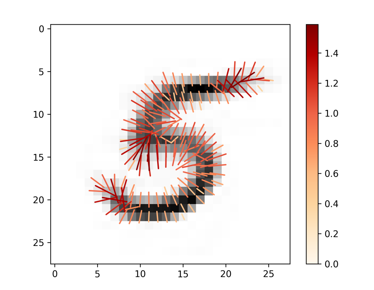
Figure 1: The final resolution measure visualized by coloured bars on top of an affine template for the sample images of handwritten digits “5” from the MNIST dataset [6]. The length and colour of the bars indicate the resolution at the corresponding locations.

Our goal is the quantification of the misalignment remaining after image registration, leading to the development of a pointwise measure of the resolution of the template generated in a groupwise registration. More specifically the misalignment of the images can be thought of to be composed of a “vertical” part corresponding to image intensity variations at the same location of a common feature and a “horizontal” part due to spatial misalignments of the features themself. While the vertical variation may be quantified by something as simple as the pixelwise standard deviation of the registered images, the horizontal variation is much harder to capture because at every pixel one has to incorporate the information of a neighbourhood of that location. The measure developed below is interpretable as a horizontal resolution of the generated template measured in pixels, see Figure 1.

Commonly used tools that quantify the alignment accuracy of a registration between images, be it groupwise or just pairwise registration, are volume overlap measures such as the Dice score/coefficient or Jaccard index [7, 2, 1]. These measures require the availability of an additional segmentation and labelling of the images and produce a single scalar per segment. This additional information is not required by our method, which even provides a pixelwise measure. In fact, our novel approach based on Gaussian smoothing of the registered images offers a simple visual way of assessing the local reliability of the template image, identifying the regions where the samples agree on a feature and quantifying those where they are horizontally misaligned.

II Background: Registration and Templates

The registration of two images consists of finding a transformation from a given class of transformations (e.g. affine) that warps one of the images such that it matches the other (fixed) image as closely as possible with respect to a suitable similarity metric.

In the following, images are given by (square integrable) functions $I:\Omega\to\mathbb{R}$ assigning to each point of the image domain $\Omega\subseteq\mathbb{R}^{d}$ a real valued intensity (grey value). The dimensions of the image domain that are considered here are $d=1,2,3$.

Note that in practice, the continuum $\Omega$ is, of course, approximated by a discrete grid of pixels and even though the registration framework below is formalized in the continuous setting, it is solved approximately for suitably discretized versions of the corresponding mathematical concepts.

The transformations acting on the images are now given by diffeomorphic (i.e. bijective and in both directions differentiable) functions $\Psi:\Omega\to\Omega$ on the image domain, which create a warped image through the expression $I\circ\Psi^{-1}$. This means that the grey value of the warped image at a point $y\in\Omega$ is given by $I(x)$ for $x=\Psi^{-1}(y)$, which is just the point that gets mapped to $y$ under $\Psi$.

A common approach for the creation of a template of $n$ images $I_{1},\dots,I_{n}$ is the minimization of a functional based on pairwise image registrations [2, 1]. Such functionals often are of the form

$$\mathcal{E}(T,\theta_{1},\dots,\theta_{n})=\sum_{i=1}^{n}\mathcal{L}_{\rm sim}(I_{i}\circ\Psi^{-1}_{\theta_{i}},T)+\lambda\,\mathcal{L}_{\rm reg}(\Psi^{-1}_{\theta_{i}})\,,$$

where an image similarity term $\mathcal{L}_{\rm sim}$ measures the discrepancy between the warped images and the template $T$ and a regularization term $\mathcal{L}_{\rm reg}$ penalizes the complexity of the transformation, thus avoiding deformations that are unnecessarily large. The terms are coupled through a trade-off parameter $\lambda>0$. Here every image $I_{i}$ has its own associated transformation $\Psi_{\theta_{i}}$ parametrized by a suitable parameter $\theta_{i}$.

A simple choice for the similarity term is the $L^{2}$-norm:

$$\mathcal{L}_{\rm sim}(I,J)=\|I-J\|_{2}^{2}=\int_{\Omega}(I(x)-J(x))^{2}\,\mathrm{d}x\,.$$

Other common choices are metrics based on (normalized) cross correlation or (normalized) mutual information [8]. Here, the $L^{2}$-norm is used due to its simplicity while the less common $L^{1}$-norm $\|I-J\|_{1}=\int_{\Omega}|I(x)-J(x)|\,\mathrm{d}x$ is also used for demonstration purposes below, as it leads to (artificially) sharper templates, see Figures 2, 5, and 6.

The regularization term $\mathcal{L}_{\rm reg}$ depends on the chosen class of transformations. We will consider the following two classes.

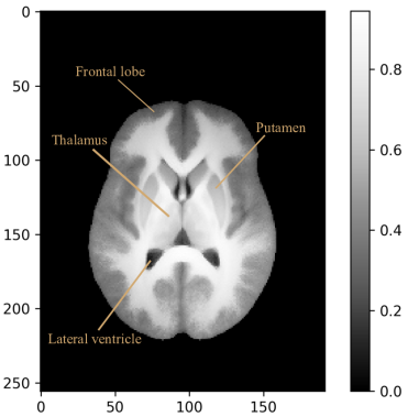
Figure 2: Horizontal slice for a sample image from the NFBS dataset [9] after registration (top) and the corresponding template (middle) based on $L^{2}$-norm similarity and affine transformations, as well as an annotated template (bottom) based on the $L^{1}$-norm similarity and affine transformations.

Affine transformations

If $\Omega=\mathbb{R}^{d}$ the transformations are called affine if they are of the from

$$\Psi_{\theta}(x)=Ax+b\,,$$

for $x\in\Omega$ and $\theta=(A,b)$ with an invertible matrix $A\in\text{GL}(d)$ and a translation vector $b\in\mathbb{R}^{d}$. Since affine maps are always defined on all of $\mathbb{R}^{d}$, it is often necessary to extend the images, e.g. by defining them to have the constant value zero outside the image domain.

Rigid transformations

If the matrix $A$ of an affine transformation is a rotation matrix $A\in\mathrm{SO}(d)$, i.e. it satisfies $A^{\mathsf{T}}A=I_{d}$ and $\det A=1$, the transformation is called rigid or an Euclidean transformation.

In both cases these affine transformations can be regularized by

$$\mathcal{L}_{\rm reg}(\Psi_{\theta})=\|A-I_{d}\|_{2}^{2}+\|b\|_{2}^{2}\,,$$

which penalizes the transformation from deviating too much from the identity transformation $\Psi_{\text{id}}(x)=x$.

More complicated non-linear transformations are commonly used to achieve state of the art registration accuracy; these are often created by integrating suitable vector fields [2, 1, 10].

As already mentioned, for real images given on a discrete domain that approximates the underlying continuum $\Omega$, the minimization is performed numerically with a discretized version of the functional $\mathcal{E}$. After minimizing $\mathcal{E}$ the optimal parameters $\hat{\theta}_{1},\dots,\hat{\theta}_{n}$ and the template $\hat{T}$ are obtained. The registered images $R_{i}=I_{i}\circ\Psi_{\hat{\theta}_{i}}^{-1}$ are now aligned with the template. Figure 2 shows an example of a registered sample image for the 3d example dataset from Subsection IV-B together with template images for the $L^{2}$- and $L^{1}$-norm for affine transformations.

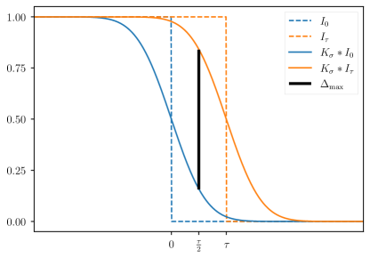
(a)

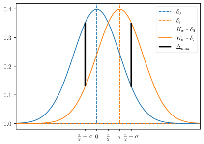
(b)

Figure 3: Behaviour of example images under Gaussian smoothing, on the left for two shifted edges and on the right for two shifted point masses. The maximal difference $\Delta_{\max}$ decreases in both cases for increasing bandwidth $\sigma$.

III Methods

The basic idea underlying our method is that smoothing, i.e. local averaging, reduces those differences between registered images which are due to horizontal variation. Therefore, the amount of smoothing necessary to make these differences small allows to quantify the horizontal misalignment.

III-A Horizontal translations under Gaussian smoothing

Given registered images with local features like edges or peaks, how do small horizontal misalignments between such features still left after registration behave under Gaussian smoothing? Gaussian smoothing can be achieved by the convolution of an image with a Gaussian kernel of a certain bandwidth $\sigma>0$, which is given in the one dimensional case by

$$K_{\sigma}(x)=\tfrac{1}{\sigma\sqrt{2\pi}}e^{-\frac{1}{2}\frac{x^{2}}{\sigma^{2}}}\,.$$

The following two stylized examples of one dimensional “images”, i.e. with spatial domain $\Omega=\mathbb{R}$, are used to study the influence of smoothing on horizontal misalignment.

Shifted edges

For a sharp edge $I_{s}(x)=\mathbf{1}_{(-\infty,s]}(x)$ (indicator function of the interval $(-\infty,s]$) at a location $s\in\mathbb{R}$ we have for the smoothed image $(K_{\sigma}*I_{s})(x)=1-\Phi(\tfrac{x-s}{\sigma})$, where $\Phi$ is the distribution function of the standard normal distribution. For two misaligned images $I_{0}$ and $I_{\tau}$ the difference of the smoothed images

$$|(K_{\sigma}*I_{0})(x)-(K_{\sigma}*I_{\tau})(x)|=|\Phi(\tfrac{x}{\sigma})-\Phi(\tfrac{x-\tau}{\sigma})|$$

attains its maximum, due to symmetry, at the location $x=\tfrac{\tau}{2}$ with the value

$$\Delta_{\max}=|2\Phi(\tfrac{1}{2}\tfrac{\tau}{\sigma})-1|\,,$$

which depends only on the ratio $\tfrac{\tau}{\sigma}$ and decreases monotonically for growing $\sigma$, see the left panel in Figure 3.

Shifted point masses

For a point mass (Dirac delta) $\delta_{s}$ at a location $s\in\mathbb{R}$ we have $(K_{\sigma}*\delta_{s})(x)=K_{\sigma}(x-s)$. Since the Gaussian kernel satisfies $K_{\sigma}(x)=\tfrac{1}{\sigma}K_{1}(\tfrac{x}{\sigma})$, the difference

$$|(K_{\sigma}*\delta_{0})(x)-(K_{\sigma}*\delta_{\tau})(x)|=|K_{\sigma}(x)-K_{\sigma}(x-\tau)|$$

between two misaligned, smoothed point masses located at $0$ and $\tau\in\mathbb{R}$ converges to zero for increasing $\sigma$ simply due to the effect of the smoothing itself. But even after rescaling by a factor of $\sigma$, which prevents the smoothed images from vanishing, the following approximation

$$\sigma|K_{\sigma}(x)-K_{\sigma}(x-\tau)| =|K_{1}(\tfrac{x}{\sigma})-K_{1}(\tfrac{x-\tau}{\sigma})|$$

$$=|\tfrac{\tau}{\sigma}\left(K_{1}^{\prime}(\tfrac{1}{\sigma}(x-\tfrac{\tau}{2}))+o(\tfrac{\tau}{\sigma})\right)|$$

$$\approx|\tfrac{\tau}{\sigma}K_{1}^{\prime}(\tfrac{1}{\sigma}(x-\tfrac{\tau}{2}))|\,,$$

obtained by a linearization at the midpoint, holds for $\sigma$ large relative to $\tau$, where the derivative of the Gaussian kernel is given by $K_{1}^{\prime}(x)=-xK_{1}(x)$. This approximation attains its maximum at the two locations $x=\tfrac{\tau}{2}\pm\sigma$ with a value of

$$\Delta_{\max}=\tfrac{1}{\sqrt{2\pi e}}|\tfrac{\tau}{\sigma}|\,,$$

which also depends only on the ratio $\tfrac{\tau}{\sigma}$; see the right panel in Figure 3.

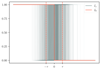
(a)

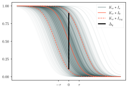
(b)

Figure 4: On the left $n=1000$ sharp edges whose shifts $s$ are randomly sampled from $\mathcal{N}(0,\tau^{2})$ are shown. On the right the samples are smoothed with bandwidth $\sigma=\tau$ and the corresponding empirical quantile range (here for the $0.1$- and $0.9$-quantile) at the location $x=0$ is shown as a bar of length $\Delta_{q}$. The smoothed versions of the edges $I_{\pm q}$ on the right belong to the $0.1$- and $0.9$-quantiles $\pm q$ of the $\mathcal{N}(0,\tau^{2})$ distribution and approximately match the endpoints of the empirical quantile range.

In both cases the maximum of the difference goes to zero for increasing $\sigma$. For the shifted edges this decrease is monotone in $\sigma$ and in the case of the smoothed point masses this behaviour also occurs for sufficiently large $\sigma$, when the above approximation becomes accurate enough. For a larger misalignment between the images, i.e. for a larger $\tau$, a larger $\sigma$ is needed in both cases to decrease the distance of the images to a given value.

More generally the misalignments that are still left between registered images can be reduced by smoothing with larger horizontal misalignments usually requiring more smoothing for the same reduction in the difference of the image intensities.

In the case of shifted edges one can now devise a strategy to quantify horizontal misalignment: since $\Delta_{\max}$ depends only on the ratio $\tfrac{\tau}{\sigma}$ one could match the strength of the smoothing with the size of the horizontal shift by choosing $\sigma=\tau$, which gives $\Delta_{\max}^{*}=2\Phi(\tfrac{1}{2})-1\approx 0.38$ independent from $\sigma$ and $\tau$. Thus, when $\tau$ is not known, two misaligned edges can be smoothed with increasing $\sigma$ until the maximum difference $\Delta_{\max}$ fulfils $\Delta_{\max}\leq\Delta_{\max}^{*}$ for the first time and the corresponding smoothing factor $\sigma^{*}$ gives an estimate of $\tau$.

For a sample of $n$ shifted edges, one can replace $\Delta_{\max}$ by a difference of two suitably chosen quantiles: if the edges are samples of a random edge $I_{S}$ with $S\sim\mathcal{N}(0,\tau^{2})$ and $p_{0},p_{1}\in(0,1)$ with $p_{0}<p_{1}$ (e.g. $p_{0}=0.1$ and $p_{1}=0.9$) are two given probabilities we want to know the resulting range of the $p_{0}$- and $p_{1}$-quantiles of the smoothed images at the location with the highest variance in the image intensities, which is at $x=0$ due to symmetry. As above, we consider the case $\sigma=\tau$, where the strength of the smoothing now matches the standard deviation of the horizontal shifts. If

$$X=(K_{\tau}*I_{S})(0)=1-\Phi(-\tfrac{S}{\tau})=\Phi(\tfrac{S}{\tau})$$

is the (random) intensity value of such a smoothed image at $x=0$ we can calculate the $p_{0}$- and $p_{1}$-quantiles of the distribution of $X$ as follows: since $\tfrac{S}{\tau}\sim\mathcal{N}(0,1)$ we have

$$\mathbf{P}(\tfrac{S}{\tau}\leq q_{k})=p_{k}$$

where $q_{k}=\Phi^{-1}(p_{k})$ for $k=0,1$ by the definition of quantiles for a continuous distribution, which can be equivalently transformed into

$$\mathbf{P}(X\leq p_{k})=p_{k}$$ (1)

since $\Phi$ is a monotonically increasing function. Thus the $p_{0}$- and $p_{1}$-quantiles of $X$ are just the values $p_{0}$ and $p_{1}$ themselves with the range $\Delta_{q}^{*}=p_{1}-p_{0}$. Another way of viewing (1) is that the distribution of $X$ is just the uniform distribution on the interval $[0,1]$.

Thus, if a sample $I_{s_{1}},\dots,I_{s_{n}}$ of shifted edges with unknown $\tau$ is smoothed until the range $\Delta_{q}$ of the empirical $p_{0}$- and $p_{1}$-quantiles of $(K_{\sigma}*I_{s_{1}})(0),\dots,(K_{\sigma}*I_{s_{n}})(0)$ satisfies

$$\Delta_{q}\leq\Delta_{q}^{*}=p_{1}-p_{0}$$ (2)

the corresponding smoothing factor $\sigma^{*}$ gives an estimate of the standard deviation $\tau$ and therefore quantifies the horizontal misalignment. This setting is visualized in Figure 4.

Instead of the quantile range $\Delta_{q}^{*}$ one could also use the standard deviation $\sqrt{\mathbf{Var}\,X}=\tfrac{1}{\sqrt{12}}$ (variance of uniform distribution) as a criterion for when to stop the smoothing, but for real images quantiles are preferred due to a higher robustness against outliers.

Algorithm 1 Template resolution measure

registered images $R_{1},\dots,R_{n}$, effective height $\eta$, threshold probabilities $(p_{0},p_{1})$, step size $s$

smoothing sigmas $\sigma^{*}(x)$ per pixel $x\in\Omega$

initialize $\sigma\leftarrow 0$, $\sigma^{*}(x)\leftarrow 0$, $\mathbf{M}(x)\leftarrow\texttt{false}$ for all $x\in\Omega$

while $\mathbf{M}(x)$ is false for any $x\in\Omega$ do $\triangleright$ run until mask $\mathbf{M}$ is true for all pixels

     for $i=1$ to $n$ do

         $S_{i}\leftarrow\textsc{GaussianFilter}(R_{i},\sigma)$ $\triangleright$ create smoothed images with bandwidth $\sigma$

     end for

     $(Q_{0},Q_{1})\leftarrow$ Quantile$(\{S_{1},\dots,S_{n}\},\{p_{0},p_{1}\})$ $\triangleright$ pixelwise empirical $p_{0}$- and $p_{1}$-quantiles of smoothed images

     $R\leftarrow(Q_{1}-Q_{0})$ $\triangleright$ pixelwise quantile range

     $\mathbf{M}_{\text{all}}\leftarrow(R\leq\eta(p_{1}-p_{0}))$ $\triangleright$ Boolean mask of all pixels with quantile range $\leq\eta(p_{1}-p_{0})$

     $\mathbf{M}_{\text{new}}\leftarrow\mathbf{M}_{\text{all}}$ and not $\mathbf{M}$ $\triangleright$ mask of pixels that fullfill the quantile range condition for the first time

     $\mathbf{M}\leftarrow\mathbf{M}$ or $\mathbf{M}_{\text{all}}$ $\triangleright$ update mask of all pixels that fullfilled the condition at least once

     for $x\in\Omega$ where $\mathbf{M}_{\text{new}}(x)$ is true do

         $\sigma^{*}(x)\leftarrow\sigma$ $\triangleright$ save current $\sigma$ for all pixels fullfilling the quantile range condition for the first time

     end for

     $\sigma\leftarrow\sigma+s$ $\triangleright$ increase $\sigma$ by stepsize $s$

end while

III-B Application to real images

In the last section the sample of edges varied around the location $x=0$ and the quantile condition (2) was only evaluated at this single location. For real images one can now determine the smallest bandwidth $\sigma^{*}$ at every location $x\in\Omega$ satisfying condition (2) at $x$. In Figure 5 this is visualized for the sample of shifted edges, where the orange line is the corresponding $\sigma^{*}$ as a function of the location $x$. This is useful as a visual way of quantifying the horizontal variability of a sample of images in a localised manner, especially when the dimension of $\Omega$ is larger than one. Here, the computed $\sigma^{*}$ values are zero wherever most samples agree on having a plateau of height zero or one and the maximum at $x=0$ corresponds to the resolution of the edge, all other values are to be understood to continuously interpolate between these two cases. For the simultaneously generated template the values $\sigma^{*}(x)$ can be interpreted as the resolution of the template at the location $x$.

Natural images, especially in more than one dimension, deviate from the model situation above, where idealized one-dimensional edges were shifted based on a Gaussian distribution, in a number of ways: edges might not be perfectly sharp; their horizontal misalignment can be caused by more complicated transformations like rotations, shearings or even non-linear deformations; and even in the translation case the Gaussian distribution assumption might be inappropriate. Additionally, edges in real images usually belong to plateaus of different heights.

Despite these challenges we use the model situation as a rule of thumb and augment the quantile range $\Delta_{q}^{*}$ by multiplying it with an additional parameter $\eta$, that can be interpreted as an effective height of the edge for which one wants to quantify the horizontal misalignment. The effective height needs to be hand-tuned to the specific sample of images under consideration, e.g. for the examples in Section IV the value of $\eta$ is chosen to be about have the intensity range. The goal range for the reduction in the quantile range is now $\eta\Delta_{q}^{*}$, since the inequality in (1) is simply scaled with $\eta$.

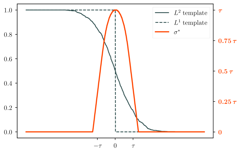
Figure 5: Based on the (sharp) edge samples from Figure 4 the smoothing bandwidth $\sigma^{*}(x)$ satisfying condition (2) is shown at each location $x$ together with the templates for the $L^{2}$- and $L^{1}$-norm (here given by the pixelwise mean and median of the sample images).

III-C Template resolution measure

Given the registered images $R_{i}=I_{i}\circ\Psi_{\hat{\theta}_{i}}^{-1}$ from Section II the remarks of the last subsection now turn into the following procedure: All registered images are progressively smoothed with increasing bandwidth $\sigma$, starting with $\sigma=0$ (original non-smoothed images). At every location $x\in\Omega$ in the image domain one now searches for the smallest bandwidth $\sigma^{*}(x)$, which decreases the difference between the empirical $p_{0}$- and $p_{1}$-quantiles of the smoothed images for given $p_{0},p_{1}\in(0,1)$ at $x$ below the $\eta\Delta_{q}^{*}=\eta(p_{1}-p_{0})$ threshold. This is also described with more detail in Algorithm 1. The resulting “image” $\sigma^{*}$ (see Figure 7 and 11) now quantifies the horizontal variation of the images registered with the template at every location of the image domain.

In the examples we assume that all images are naturally extended beyond $\Omega$ by defining the intensity to be zero there. This choice also guarantees the convergence of the above procedure, since such images vanish under Gaussian smoothing for sufficiently large $\sigma$ (similar to the model situation with the point masses) and will eventually fulfil the quantile condition everywhere.

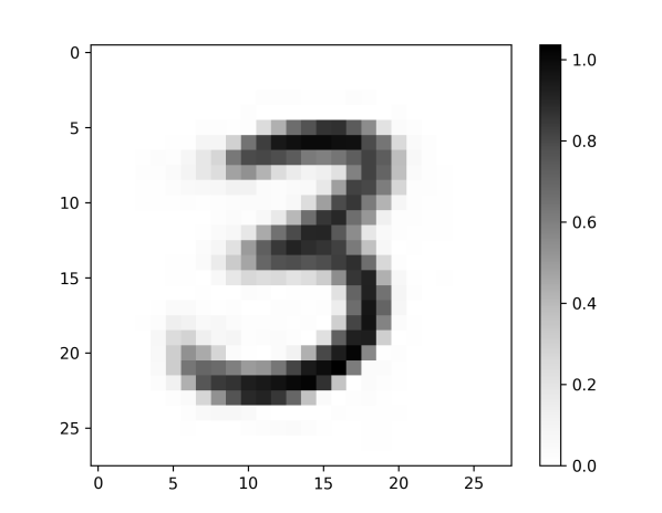
(a)

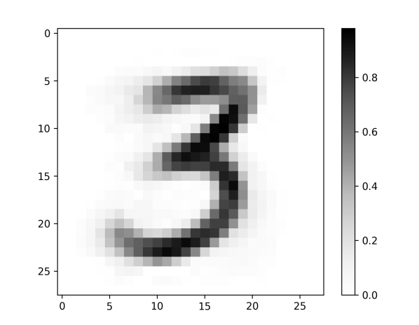
(b)

(c)

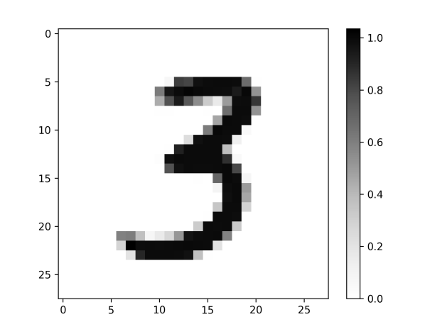
(d)

Figure 6: Templates for the digit 3 from the MNIST dataset [6] based on the $L^{2}$-norm (top row) and the $L^{1}$-norm (bottom row) for affine (left column) and rigid (right column) transformations.

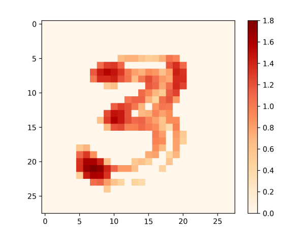
(a)

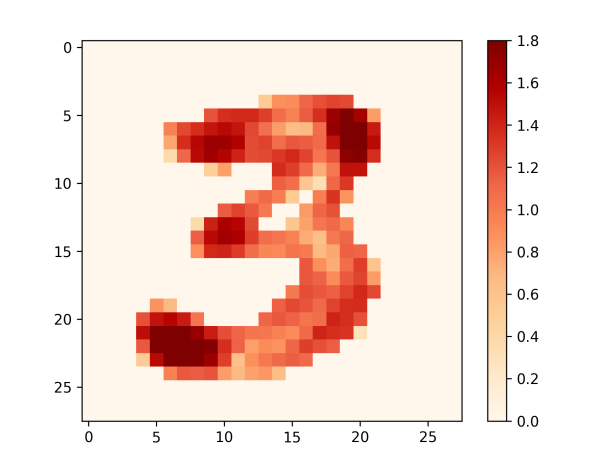
(b)

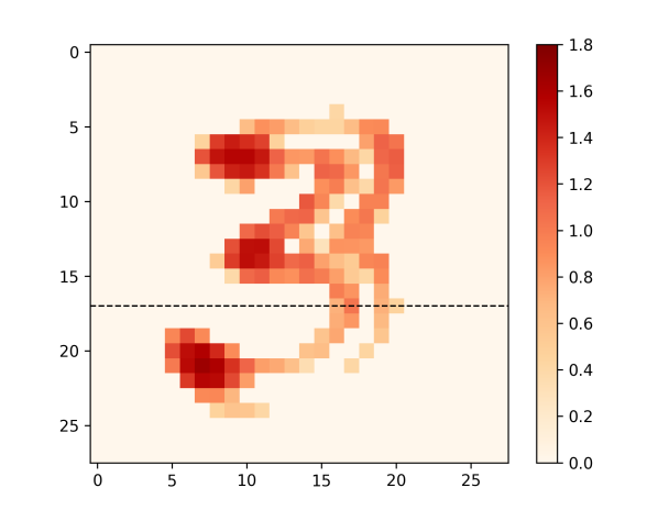
(c)

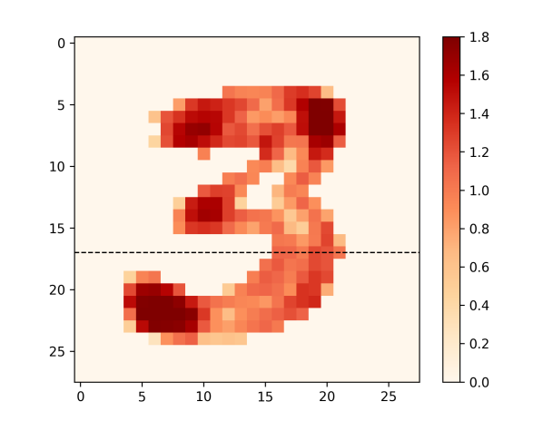
(d)

Figure 7: Template resolution measure $\sigma^{*}$ based on the $L^{2}$-norm (top row) and the $L^{1}$-norm (bottom row) for affine (left column) and rigid (right column) transformations. Figure 9 shows 1d slices (dashed lines in the bottom row) for the $L^{1}$ case.

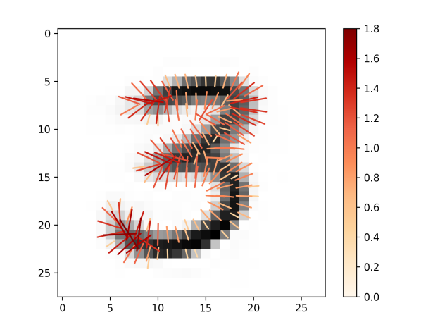
(a)

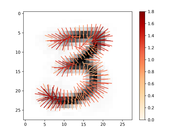
(b)

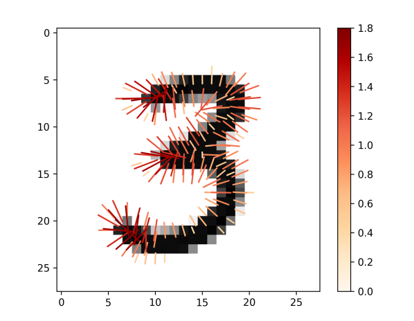
(c)

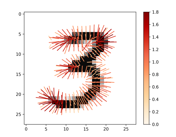
(d)

Figure 8: Visualization of $\sigma^{*}$ on top of the templates based on the $L^{2}$-norm (top row) and the $L^{1}$-norm (bottom row) for affine (left column) and rigid (right column) transformations.

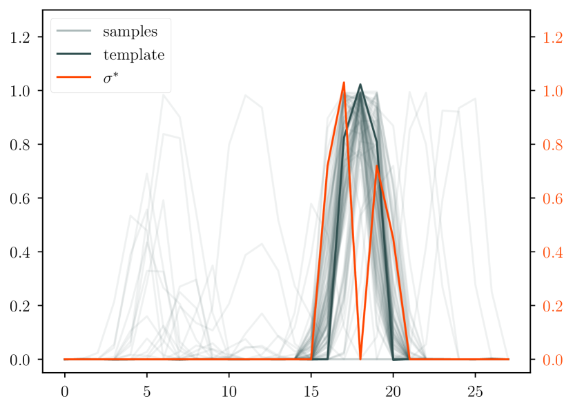
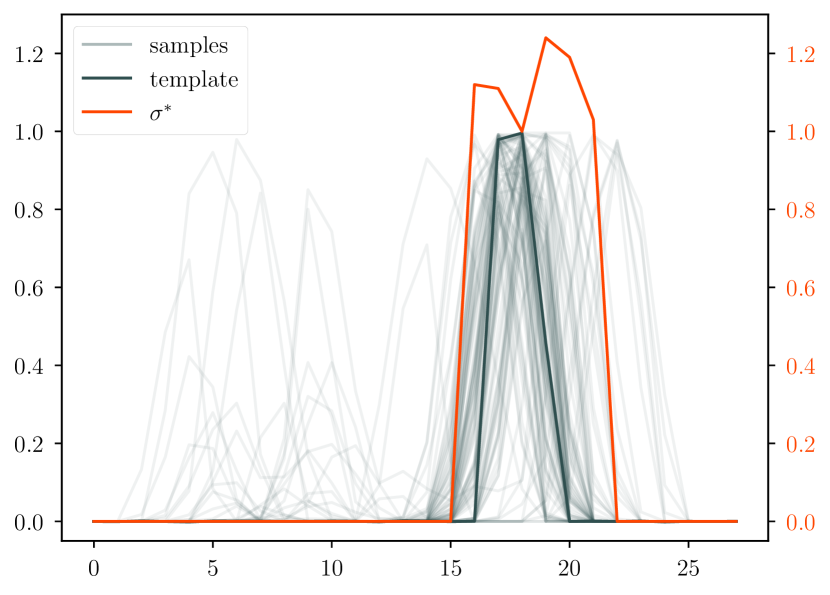
Figure 9: One dimensional slices of $\sigma^{*}$ (along the dashed lines in Figure 7) for the template based on the $L^{1}$-norm and affine (top) or rigid (bottom) transformations. The corresponding templates and registered samples are also shown.

III-D Visualization of the template resolution

Since the values of $\sigma^{*}$ quantify the horizontal resolution of the template $T$, a visualization of the $\sigma^{*}(x)$ values on top of the template at the corresponding locations is desired. For this, at every pixel location $x\in\Omega$ of the template the gradient $\nabla T(x)$ is estimated (e.g. via a Gaussian derivative filter). The value $\sigma^{*}(x)$ ist then visualized as a bar of length $2\,\sigma^{*}(x)$ centred at $x$ along the direction given by $\nabla T(x)$, as shown in Figure 1, 8 and 12. When the gradient $\nabla T(x)$ is zero at $x$ no bar is plottet. In the 3d case the bar is projected orthogonally onto the plane of the 2d image slice being visualized. The gradient direction is a natural choice for displaying the horizontal variation in so far as it is orthogonal to the level sets of the template image and thus the horizontal variation at a point on an edge of the template is also visualized orthogonal to this edge.

IV Experiments

Algorithm 1 is now used to analyse two example datasets in two and three dimensions. The threshold probabilities $p_{0}$ and $p_{1}$ are always chosen as $0.1$ and $0.9$, respectively, i.e., 80% of the smoothed images are required to deviate from each other by at most 80% of the effective height $\eta$.

IV-A 2d digits

First, the classic MNIST dataset [6] is used to demonstrate the method on a relatively simple collection of 2d images. The image intensities are all normalized to the range $[0,1]$ and the effective height $\eta\approx 0.6$, i.e. 60% of the intensity range, is chosen such that the resulting visualization in Figure 8 is not too cluttered.

For the first $100$ samples of each type of digit in the dataset a groupwise registration and template generation was performed. Here the images of the digit 3 are registered with affine and rigid transformations and with the $L^{2}$- and $L^{1}$-norm as similarity metrics. The resulting templates are shown in Figure 6, where one can see that the $L^{1}$-norm templates appear sharper than the corresponding $L^{2}$-norm versions, but the template resolution measure given by Algorithm 1 shows that the horizontal variability of the registered digits is actually similar in both cases. The resolution values $\sigma^{*}$ are shown in Figure 7 and the visualization proposed in Section III-D is shown on top of the templates in Figure 8. As expected, the affine transformations lead to a better registration than the rigid ones. Here we can see that the horizontal variation quantified by $\sigma^{*}$ is in accordance with what one would expect in the case of handwritten digits, in particular the position of the end pieces (where the pen is first put down or lifted) and the corner where the arcs meet are highly uncertain in contrast to the top of the upper arc and the curving part of the bottom arc (which are the features the digits are aligned on during the registration).

In Figure 9 one dimensional slices (along the dashed lines in Figure 7) through the resolution measures (together with the templates and the registered sample images) are shown for the $L^{1}$-norm (slices for the $L^{2}$-norm look similar). Here one can see that the misalignments quantified by $\sigma^{*}$ are in good correspondence with the visible misalignments of the sample images, e.g. the samples are less aligned with the right slope of the rigid template (bottom) than in the affine version (top), and the size of the misalignment is consistent with the value of $\sigma^{*}$ at that location.

The digit dataset was also used to examine the robustness of the resolution measure to changes in the probability thresholds $p_{0}$ and $p_{1}$, which showed that a quantile range ($p_{1}-p_{0}$) between 0.7 and 0.9 gives qualitatively similar results as the choice $p_{0}=0.1$ and $p_{1}=0.9$ (data not shown).

IV-B 3d brains

An important application of image registration is the preprocessing of 3d MRI brain images. Here a collection of brain images (possibly from different subjects) are registered with a template, here also called an atlas, which enables more direct comparisons between different brains despite differences in the respective brain geometry before registration. The dataset used here for demonstration purposes is the Neurofeedback Skull-stripped (NFBS) dataset [9], which contains 125 raw MRIs and their skull stripped versions. The intensities of the sample images are normalized such that the median of each image (without the background zeros) is mapped to $0.5$. Additionally, we are optimizing an intensity scaling factor for each image during the registration such that the scaled template matches the registered image under the similarity metric. This minimizes the vertical variability and brings us a bit closer to the model situation of the shifted edges. The effective height for the resolution measure is chosen as $\eta\approx 0.4$.

For the skull stripped brains a template is generated for affine and rigid transformations and for $L^{2}$- and $L^{1}$-norm similarity measures, as shown in Figure 10. In each of the four cases the template resolution is computed with Algorithm 1 and horizontal slices of the resulting 3d images of the $\sigma$ values are shown in Figure 11 and visualized on top of the template, as described in Subsection III-D, in Figure 12.

Again, the affine registration is more accurate, especially at the boundary of the brain, and the $L^{1}$-norm templates appear sharper than the $L^{2}$-norm versions but – as revealed by the template resolution measure – are only slightly better in terms of registration accuracy. The rigid registration results are almost identical. In the affine case the $L^{1}$-norm leads to better registration at the upper part of the brain (frontal lobe; see Figure 2 for locations), while being similarly inaccurate around the lateral ventricles (twin holes in the lower middle). In all cases the regions in the upper middle of the brain (around the putamen and thalamus) are quite well registered and are also the sharpest regions of the templates across all registration variants. This is in agreement with measurements of the volumes of these brain regions (see e.g. Table 4 in [11] for healthy controls, or Table 2 in [12]) where the coefficients of variation (standard deviation divided by the mean) of the volumes are relatively low for the putamen and thalamus compared with those for the lateral ventricles, the latters’ variability ranging among the highest across all measured regions.

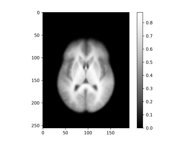
(a)

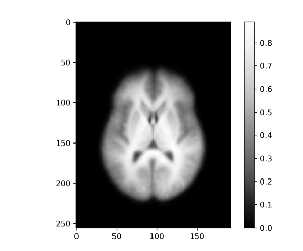
(b)

(c)

(d)

Figure 10: Horizontal slices of the templates for the 3d NFBS dataset [9] based on the $L^{2}$-norm (top row) and the $L^{1}$-norm (bottom row) for affine (left column) and rigid (right column) transformations.

V Code Availability

The template resolution measure (Algorithm 1) was implemented in Python; the source code is made publicly available on GitHub (https://github.com/Stochastik-TU-Ilmenau/image-template-resolution). This includes the code to download the datasets for the two examples above and for carrying out the corresponding analyses, thus allowing to completely reproduce the results shown.

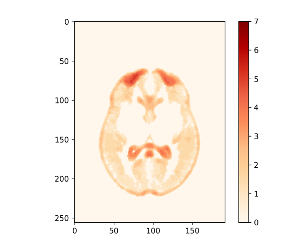
(a)

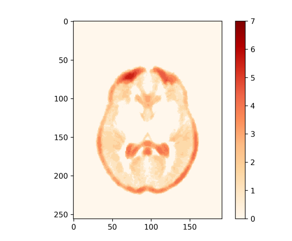
(b)

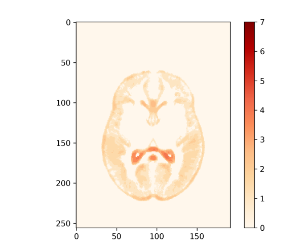
(c)

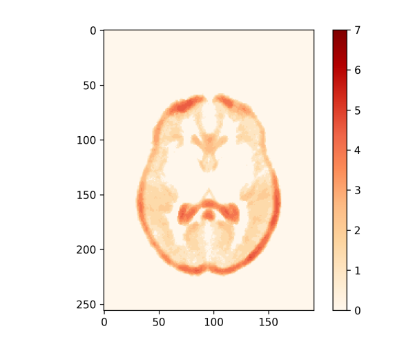
(d)

Figure 11: Template resolution measure $\sigma^{*}$ based on the $L^{2}$-norm (top row) and the $L^{1}$-norm (bottom row) for affine (left column) and rigid (right column) transformations.

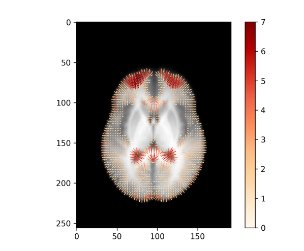
(a)

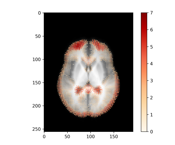
(b)

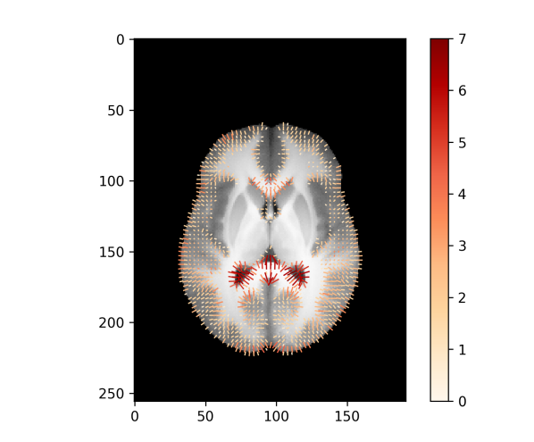
(c)

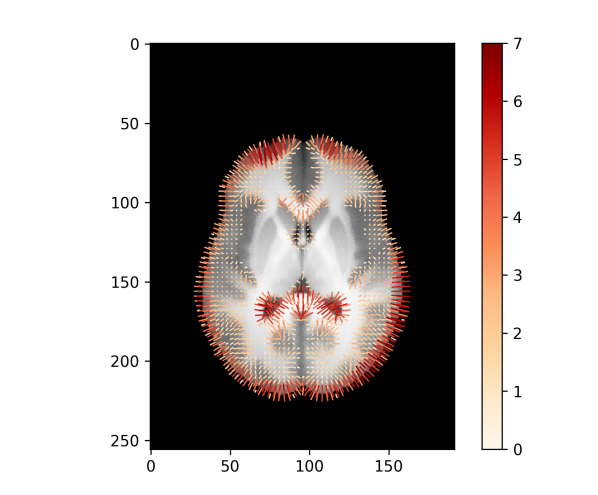
(d)

Figure 12: Visualization of $\sigma^{*}$ on top of the templates based on the $L^{2}$-norm (top row) and the $L^{1}$-norm (bottom row) for affine (left column) and rigid (right column) transformations.

VI Discussion and Conclusion

From the theoretical analyses as well as the experiments presented above, we conclude that the proposed resolution measure allows to quantify and visualize the horizontal uncertainty remaining after registration at each location of the template. In fact, in both applications the obtained measure of horizontal variability, given in the template’s units of length, is in agreement with otherwise obtained measures of the respective variability.

A major advantage of the proposed method is that it uses only the registered images as input, see Algorithm 1; in particular, no labelling or segmentation is required (cf. the last paragraph of Section I on the state of the art). The computation and visualization of the proposed resolution measure can thus be fully automatized given three parameters, namely the effective height $\eta$, as well as the threshold probabilities $p_{0}$ and $p_{1}$. However, further experiments implied that changing the threshold probabilities barely affects the results; hence, their selection is more a matter of the corresponding quantiles’ statistical robustness given the sample size. Choosing the effective height is somewhat more important, but fortunately, it has a well specified meaning as the height of a sharp edge which is to be detected as such. Therefore, about half the difference between the intensity of foreground and background will often be a reasonable choice for $\eta$.

Of course, there are situations where the proposed resolution measure’s behaviour differs from the intended one. Indeed, large values may not only correspond to horizontally misaligned features, but also to a feature mismatch, where some sample images contain a certain feature which the other samples are lacking. But even in this case the measure is useful as low values still correctly identify regions where the samples agree.

In summary, we developed a new tool to help with the evaluation of images registered groupwise to a template, providing insight into the reliability of the structures visible in the template, and quantifying as well as visualizing this in terms of a local resolution measure.

References

- [1] S. Joshi, B. Davis, M. Jomier, and G. Gerig, “Unbiased diffeomorphic atlas construction for computational anatomy,” NeuroImage, vol. 23, pp. S151–S160, 2004, mathematics in Brain Imaging. [Online]. Available: https://www.sciencedirect.com/science/article/pii/S1053811904003842
- [2] Z. Ding and M. Niethammer, “Aladdin: Joint atlas building and diffeomorphic registration learning with pairwise alignment,” in 2022 IEEE/CVF Conference on Computer Vision and Pattern Recognition (CVPR), 2022, pp. 20 752–20 761.
- [3] G. Wu, P.-T. Yap, Q. Wang, and D. Shen, “Groupwise registration from exemplar to group mean: extending hammer to groupwise registration,” in 2010 IEEE International Symposium on Biomedical Imaging: From Nano to Macro. IEEE, 2010, pp. 396–399.
- [4] P. Lorenzen, B. C. Davis, and S. Joshi, “Unbiased atlas formation via large deformations metric mapping,” in Medical Image Computing and Computer-Assisted Intervention–MICCAI 2005: 8th International Conference, Palm Springs, CA, USA, October 26-29, 2005, Proceedings, Part II 8. Springer, 2005, pp. 411–418.
- [5] A. Legouhy, F. Rousseau, C. Barillot, and O. Commowick, “An iterative centroid approach for diffeomorphic online atlasing,” IEEE Transactions on Medical Imaging, vol. 41, no. 9, pp. 2521–2531, 2022.
- [6] Y. LeCun, C. Cortes, and C. Burges, “Mnist handwritten digit database,” ATT Labs, vol. 2, 2010. [Online]. Available: http://yann.lecun.com/exdb/mnist
- [7] W. R. Crum, O. Camara, and D. L. Hill, “Generalized overlap measures for evaluation and validation in medical image analysis,” IEEE transactions on medical imaging, vol. 25, no. 11, pp. 1451–1461, 2006.
- [8] M. Holden, D. L. Hill, E. R. Denton, J. M. Jarosz, T. C. Cox, T. Rohlfing, J. Goodey, and D. J. Hawkes, “Voxel similarity measures for 3-d serial mr brain image registration,” IEEE transactions on medical imaging, vol. 19, no. 2, pp. 94–102, 2000.
- [9] B. Puccio, J. P. Pooley, J. S. Pellman, E. C. Taverna, and R. C. Craddock, “The preprocessed connectomes project repository of manually corrected skull-stripped T1-weighted anatomical MRI data,” GigaScience, vol. 5, no. 1, 10 2016, s13742-016-0150-5. [Online]. Available: https://doi.org/10.1186/s13742-016-0150-5
- [10] G. Balakrishnan, A. Zhao, M. R. Sabuncu, J. Guttag, and A. V. Dalca, “Voxelmorph: a learning framework for deformable medical image registration,” IEEE transactions on medical imaging, vol. 38, no. 8, pp. 1788–1800, 2019.
- [11] D. Weinberg, R. Lenroot, I. Jacomb, K. Allen, J. Bruggemann, R. Wells, R. Balzan, D. Liu, C. Galletly, S. V. Catts, C. S. Weickert, and T. W. Weickert, “Cognitive Subtypes of Schizophrenia Characterized by Differential Brain Volumetric Reductions and Cognitive Decline,” JAMA Psychiatry, vol. 73, no. 12, pp. 1251–1259, 12 2016.
- [12] H. Soysal, N. Acer, M. Özdemir, and Ö. Eraslan, “Volumetric measurements of the subcortical structures of healthy adult brains in the turkish population,” Folia Morphologica, vol. 81, no. 2, pp. 294 – 306, 2022.