Optimal shielding for Einstein gravity

Abstract

In order to construct asymptotically Euclidean, Einstein’s initial data sets, we introduce the localized seed-to-solution method and establish the existence of classes of data sets that exhibit the gravity shielding phenomenon (or localization). We achieve optimal shielding in the sense that the gluing domain can be a collection of arbitrarily narrow nested cones while the metric and extrinsic curvature may be controlled at a super-harmonic rate, and may have arbitrarily slow decay (possibly beyond the standard ADM formalism). We also uncover several notions of physical and mathematical interest: normalized asymptotic kernel elements, localized energy functionals, localized ADM modulators, and relative energy-momentum vectors.

• February 2024

1 Shielding phenomena in Einstein gravity

Shielding.

We consider $n$-dimensional initial data sets for Einstein’s vacuum field equations of general relativity, namely spacelike hypersurfaces embedded in a vacuum spacetime, modeled by a Ricci flat, $(n+1)$-dimensional Lorentzian manifold. Einstein’s constraints form a set of $n+1$ differential equations for the induced intrinsic geometry and extrinsic geometry. An extensive literature in physics and in mathematics is available on the construction of physically meaningful classes of solutions. In particular, one important strategy referred to as the variational method was introduced by Corvino [10] and Corvino and Schoen [12] —who built on Fischer and Marsden’s work of the deformations of the scalar curvature operator.

Motivated by the study of isolated gravitational systems, we are interested here in asymptotically Euclidean, initial data sets and in the so-called anti-gravity or shielding phenomenon. Recall that, by the positive mass theorem, any vacuum space that coincides with the Euclidean space in the vicinity of an asymptotically Euclidean end is, in fact, globally isometric to the Euclidean space. In [6], Carlotto and Schoen made a remarkable discovery by distinguishing between different angular directions at infinity. Namely, there exist non-trivial solutions to the constraints that, in a neighborhood of infinity, coincide with the Euclidean geometry in all angular directions except within a conical domain with possibly arbitrarily small angle. Alternatively, the Euclidean and the Schwarzschild solutions can be picked up at infinity and be glued together across a conical domain. Chruściel and Delay [8, 9, 14] presented a method that applied to more general gluing domains and manifolds with hyperbolic ends. (Cf. the reviews [5, 7, 15] and Section 6, below.) In this Letter, we follow this line of investigation. Other recent important advances on the gluing problem include [1, 2, 11, 13, 23] and further references are cited throughout this text.

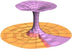
(a) (b) (c)

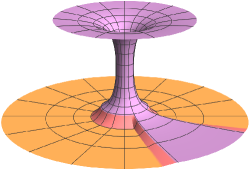
Figure 1: Euclidean metric (orange) glued to the Schwarzschild metric (purple) across a region that is conical at infinity. (a) Exact sub-harmonic localization. (b) Asymptotic super-harmonic localization. (c) Exact super-harmonic localization.

Asymptotic shielding.

The gluing scheme proposed by Carlotto and Schoen [6] allowed them to establish sub-harmonic estimates within the localization region, namely estimates in $r^{-n+2+\eta}$ with respect to a radial coordinate $r$ at infinity for arbitrarily small exponent $\eta>0$. Their result is illustrated in Figure 1(a). Carlotto and Schoen conjectured that the localization with harmonic estimates should be achievable, that is, with $\eta=0$. Next, P. LeFloch and Nguyen [21, 22] proposed a different approach to the gluing problem and formulated what they called the asymptotic localization problem, as opposed to the exact version in [6]. The notion of seed-to-solution map (cf. Section 2, below) was also introduced and sharp estimates at the (super-)harmonic level of decay were established, so that the gluing at (super-)harmonic rate was achieved in the sense that solutions enjoy the behavior required by the seed data in all angular directions at harmonic level at least, up to contributions with much faster radial decay. This result is illustrated in Figure 1(b).

Optimal shielding.

In contrast with [6, 22], in [20], reported in this Letter, we are now able to achieve (super-)harmonic control together with the exact localization sought by Carlotto and Schoen in their conjecture —as well as other “optimal” features discussed next. The optimal localization theory, as we call it, is based on the notion of localized seed-to-solution projection, a notion we outline in Section 2, below. Our method allows for the construction of broad classes of solutions which are of physical interest, and provide an approximation scheme readily applicable for computational simulations. It is based on a combination of physical insights, geometric analysis techniques, including the study of the (linear and nonlinear) structure of the Einstein constraint equations. More precisely, we construct classes of solutions that

• are defined by gluing within conical domains, possibly nested with narrow angles,

• may have arbitrarily slow decay, possibly with infinite ADM energy, and

• enjoy (super-)harmonic decay estimates.

For a schematic illustration of the decay we refer to Figure 1(c). In the course of our study, we uncover several notions of physical and mathematical interest: normalized asymptotic kernel elements, localized energy functionals, localized ADM modulators, and relative energy-momentum vectors. Importantly, this theory provides us with a complete and direct validation of Carlotto and Schoen’s conjecture. We now outline the concepts leading to (i)–(iii) above, while referring to our companion paper [20] for further technical details and applications.

2 Localized seed-to-solution projection

Einstein constraints.

For $n\geq 3$, we are interested in $n$-dimensional Riemannian manifolds $(\mathcal{M},g,k)$ with (one or) several asymptotic ends, endowed with a Riemannian metric $g$ and a symmetric $(0,2)$-tensor field $k$, and instead of working with $k$ directly we consider the $(2,0)$-tensor $h$ defined by

$$h=\big{(}k-\Tr_{g}(k)g\big{)}^{\sharp\sharp},$$ (1)

where the sharp symbol refers to the duality between covariant and contravariant tensors induced by $g$. The Hamiltonian and momentum constraints in vacuum read

$$\mathcal{H}(g,h)=R_{g}+{1\over n-1}\bigl{(}\Tr_{g}h\bigr{)}^{2}-|h|^{2}_{g}=0,\qquad\mathcal{M}(g,h)=\textnormal{{Div}}_{g}h=0,$$ (2)

in which $R_{g}$ denotes the scalar curvature of $g$, and $\Tr_{g}h$ and $|h|_{g}$ denote the trace and norm of $h$, respectively, while $\textnormal{{Div}}_{g}$ stands for the divergence operator.

From seed data to initial data sets.

We introduce a parametrization of all solutions in the “vicinity” of a given localization data set, as we call it, which serves to specify the underlying geometry of interest, that is, both the gluing domain and the asymptotic decay profile. A localization domain $\Omega\subset\mathcal{M}$ is provided, together with a weight

$$\omega_{p}=\lambda^{P}r^{n/2-p}.$$ (3)

In each asymptotic end, this weight specifies a localization in angular directions based on a function $\lambda\geq 0$ vanishing linearly on the boundary of $\Omega$, raised to some large enough power $P$, and also contains the factor $r^{n/2-p}$ concerning the radial decay in spacelike directions. Moreover, a “reference” data set $(g_{0},h_{0})$ is chosen which plays a secondary role in our construction (and satisfies the decay condition (8), below). Our parametrization is presented in terms of a localized seed-to-solution, variational projection operator, as we call it, which is denoted by

$$\eqalign{\textnormal{{Sol}}^{\lambda}_{n,p}\colon{}&(g_{\scriptsize\textrm{seed}},h_{\scriptsize\textrm{seed}})\in\textbf{seed}(\Omega,g_{0},h_{0},p_{\mathrm{G}},p_{\mathrm{A}},\epsilon)\\ &\mapsto(g,h)\in[(g_{\scriptsize\textrm{seed}},h_{\scriptsize\textrm{seed}})],}$$ (4)

and which maps seed data sets $(g_{\scriptsize\textrm{seed}},h_{\scriptsize\textrm{seed}})$ to “exact” data sets solving the Einstein constraints. This standpoint extends the (non-localized) formulation in [22]. The characterization of the projection is given in (6)–(7), below, and $[(g_{\scriptsize\textrm{seed}},h_{\scriptsize\textrm{seed}})]$ stands for the equivalence class associated by this projection.

Decay exponents: projection, geometry, and accuracy.

We focus on the class of asymptotically Euclidean solutions and the gluing within a domain $\Omega$ with asymptotically conical domains described in certain preferred charts at infinity. It is essential to clearly distinguish between the roles (and the ranges) of several pointwise decay exponents denoted by $p,p_{\mathrm{G}},p_{\mathrm{A}}$ and satisfying

$$p\in(p^{\flat}_{n},n-2),\qquad p_{\mathrm{G}}\in(0,+\infty),\qquad p_{\mathrm{A}}\geq\max(p,p_{\mathrm{G}}),$$ (5)

where $p^{\flat}_{n}=\frac{1}{2}(n-2-1/(n-2))$.

• The projection exponent $p$ for the map $\textnormal{{Sol}}^{\lambda}_{n,p}$ arises in the variational formulation of the linearized Einstein operator. In short, we seek a deformation of the form

  $$g=g_{\scriptsize\textrm{seed}}+\gamma,\qquad h=h_{\scriptsize\textrm{seed}}+\eta,$$ (6)

  where, up to weights, $(\gamma,\eta)$ belongs to the image of the adjoint $\rmd\mathcal{G}_{(g_{0},h_{0})}^{*}$ of the linearization —at the reference point $(g_{0},h_{0})$— of the Hamiltonian and momentum operators (1). Specifically, there exist a scalar field $u$ and a vector field $Z$ so that

  $$\gamma=\omega_{p}^{2}\,\rmd\mathcal{H}_{(g_{0},h_{0})}^{*}[u,Z],\qquad\eta=\omega_{p+1}^{2}\,\rmd\mathcal{M}_{(g_{0},h_{0})}^{*}[u,Z].$$ (7)

• The geometry exponent $p_{\mathrm{G}}$ specifies the (possibly very low) decay of the seed metric and extrinsic curvature $(g_{\scriptsize\textrm{seed}},h_{\scriptsize\textrm{seed}})$ relative to Euclidean data $(\delta,0)$, namely

  $$g_{\scriptsize\textrm{seed}}-\delta=\Or(r^{-p_{\mathrm{G}}}),\qquad h_{\scriptsize\textrm{seed}}=\Or(r^{-p_{\mathrm{G}}-1}).$$ (8)

• The accuracy exponent $p_{\mathrm{A}}$ describes how well the seed data obeys the constraints in the vicinity of each asymptotic end, in the sense that

  $$\mathcal{H}(g_{\scriptsize\textrm{seed}},h_{\scriptsize\textrm{seed}})=\Or(\lambda^{P}r^{-p_{\mathrm{A}}-3}),\qquad\mathcal{M}(g_{\scriptsize\textrm{seed}},h_{\scriptsize\textrm{seed}})=\Or(\lambda^{P}r^{-p_{\mathrm{A}}-3}).$$ (9)

Rigorous results are stated in suitably weighted and localized Lebesgue-Hölder norms, which we omit in this Letter and require dealing with Killing initial data sets [25]. The above conditions are sufficient in order to establish the existence of the projection map $\textnormal{{Sol}}^{\lambda}_{n,p}$ in (4) together with sub-harmonic estimates, as discovered in [6] and slightly extended in [20].

3 Optimal shielding from within narrow gluing domains

Harmonic stability.

Our main observation concerns the derivation of sharp integral and pointwise estimates, which involve (cf. (10))

• the sharp decay exponent $p_{\star}\in(n-2,p_{n,p}^{\boldsymbol{\lambda}})$ with $p_{\star}\leq p_{\mathrm{A}}$, which controls how the difference $(g-g_{\scriptsize\textrm{seed}},h-h_{\scriptsize\textrm{seed}})$ between the seed data set and actual solution decays.

Here, $p_{n,p}^{\boldsymbol{\lambda}}$ denotes an upper bound exponent which is super-harmonic and generally depends upon the localization function $\lambda$. When applying the projection operator $\textnormal{{Sol}}^{\lambda}_{n,p}$, we discover that ${(g_{\scriptsize\textrm{seed}},h_{\scriptsize\textrm{seed}})-(g,h)}$ contains a harmonic contribution as part of the asymptotic structure of the solution at each asymptotic end. Namely, by examining an asymptotic version of the constraints at infinity (cf. Section 4), we unveil certain (asymptotic kernel) contributions associated with the sphere at infinity (cf. Section 5).

Overview of the main theorem.

We only state here an informal version of our main conclusion. Consider a conical localization data set $(\mathcal{M},\Omega,g_{0},h_{0},r,\lambda)$ together with (projection, geometry, accuracy) exponents $(p,p_{\mathrm{G}},p_{\mathrm{A}})$, as stated earlier. Assume the localization function $\lambda$ satisfies, at each asymptotic end, suitably weighted Poincaré and Hardy-type inequalities which express certain Hamiltonian and momentum stability conditions restricted to the $(n-1)$-dimensional sphere at infinity.

• For any localized seed data set $(g_{\scriptsize\textrm{seed}},h_{\scriptsize\textrm{seed}})$ that is sufficiently close to $(g_{0},h_{0})$, there exists a solution $(g,h)$ to the Einstein constraints defined in (6)–(7) by variational projection of $(g_{\scriptsize\textrm{seed}},h_{\scriptsize\textrm{seed}})$ which enjoys the pointwise decay estimates

  $$g=g_{\scriptsize\textrm{seed}}^{\scriptsize\textrm{mod}}+\Or(\lambda^{\underline{P}}r^{-p_{\star}}),\qquad h=h_{\scriptsize\textrm{seed}}^{\scriptsize\textrm{mod}}+\Or(\lambda^{\underline{P}}r^{-p_{\star}-1})$$ (10)

  for some large exponent $\underline{P}$ with $\underline{P}<P$.

• In (10), the modulated seed data set $(g_{\scriptsize\textrm{seed}}^{\scriptsize\textrm{mod}},h_{\scriptsize\textrm{seed}}^{\scriptsize\textrm{mod}})$, as we call it, is defined in (17)–(19), below, and coincides with the prescribed seed data set $(g_{\scriptsize\textrm{seed}},h_{\scriptsize\textrm{seed}})$ up to “modulators” belonging to the finite-dimensional kernels of the harmonic operators associated with the Hamiltonian and momentum operators; cf. Section 5, below.

• Importantly, the Poincaré and Hardy stability conditions required on the localization function $\lambda$ allows for gluing domains that are possibly nested and arbitrarily narrow in one direction, as illustrated by Figure 2.

We refer to these results as the optimal shielding theory, since we allow for solutions that are arbitrarily localized, are generated from data with arbitrarily slow decay, and yet enjoys estimates at the super-harmonic level of decay. The interested reader should refer to [20, Theorem 1.1] for the details. In the rest of this text we present several key notions of our method.

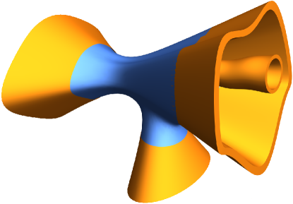
Figure 2: Example of a gluing domain with four asymptotic ends (orange) diffeomorphic to thin truncated cones, and connected by an interior region (blue).

4 Harmonic-spherical decompositions and stability conditions

Notation.

After a suitable reduction to one asymptotic end (labelled $\iota$) and by treating various terms as asymptotic perturbations, we are led to consider a single truncated conical domain $\omega_{\iota}\simeq\Omega_{R}$ of the Euclidean space $(\mathbb{R}^{n},\delta)$, consisting of a cone in $\mathbb{R}^{n}$ with a support denoted by $\Lambda_{\iota}\subset S^{n-1}$, intersected by the exterior of a ball with radius $R>0$. The weight $\omega_{\iota p}=\bigl{(}\lambda_{\iota}(x/r)\bigr{)}^{P}r^{n/2-p}$ decays as the radial distance $r\geq R$ approaches infinity, and the weight $\lambda_{\iota}$ vanishes linearly near the boundary of its support $\Lambda_{\iota}$. The localization exponent $P$ should be sufficiently large, and the projection exponent $p\in(0,n-2)$. The weighted Sobolev space $H^{2}_{-P}(\Lambda_{\iota})$ (used in (16), below) is defined with respect to the measure $\rmd\chi_{\iota}=\lambda_{\iota}^{2P}\rmd\widehat{x}$ where $d\widehat{x}$ is the standard volume form of the $(n-1)$-dimensional unit sphere $S^{n-1}$. The weighted average of a function $f\colon\Lambda_{\iota}\to\mathbb{R}$ is denoted by

$$\langle f\rangle_{\iota}=\fint_{\Lambda_{\iota}}f\,\rmd\chi_{\iota}={1\over\textnormal{Area}^{\lambda_{\iota}}}\int_{\Lambda_{\iota}}f\,\rmd\chi_{\iota},\qquad\textnormal{Area}^{\lambda_{\iota}}=\int_{\Lambda_{\iota}}\,\rmd\chi_{\iota}.$$ (11)

A decomposition of the Einstein constraints.

The asymptotic properties of the seed-to-solution map are controlled by the linearization of the constraints around Euclidean data, evaluated on the deformation $(\gamma,\eta)$ given in (7). This leads to fourth- and second-order (squared) localized Hamiltonian and momentum operators

$$\eqalign{\mathscr{H}^{\lambda_{\iota}}[u]=\omega_{\iota p}^{-2}\,\Bigl{(}(n-1)\,\Delta(\omega_{\iota p}^{2}\,\Delta u)+\partial_{i}\partial_{j}(\omega_{\iota p}^{2})\partial_{i}\partial_{j}u-\Delta(\omega_{\iota p}^{2})\Delta u\Bigr{)},\\ \mathscr{M}^{\lambda_{\iota}}[Z]^{i}=-\frac{1}{2}\,(\Delta Z^{i}+\partial_{j}\partial_{i}Z^{j})-(\partial_{j}\log\omega_{\iota,p+1})\,(\partial_{j}Z^{i}+\partial_{i}Z^{j}),}$$ (12)

in which $u\colon\Omega_{R}\to\mathbb{R}$ is scalar-valued and $Z\colon\Omega_{R}\to\mathbb{R}^{n}$ is vector-valued, and where repeated indices are implicitly summed. In the present discussion, let us focus our attention on the Hamiltonian. For the study of the (super-)harmonic decay of solutions, we introduce the following harmonic-spherical decomposition, as we call it,

$$r^{4}\mathscr{H}^{\lambda_{\iota}}[u]=\mathcal{A}[u]+\not{\mathcal{A}}^{\lambda_{\iota}}[u]+\not{\not{\mathcal{A}}}^{\lambda_{\iota}}[u].$$ (13)

The part $\mathcal{A}[u]$ contains only radial derivatives, while the “double slashed” operator is defined by plugging functions $\nu\,r^{-2(n-2-p)}$ (harmonic contributions to the metric):

$$\not{\not{\mathcal{A}}}{}^{\lambda_{\iota}}[\nu]=r^{2(n-p)}\mathscr{H}^{\lambda_{\iota}}[\nu\,r^{-2(n-2-p)}],$$ (14)

which is an elliptic but non-self-adjoint operator. Integrating it against $\nu\,\rmd\chi_{\iota}$ yields the corresponding quadratic functional

$$\not{\not{\mathrm{A}}}^{\lambda_{\iota}}[\nu]=\fint_{\Lambda_{\iota}}\Bigl{(}(n-2)(\not{\Delta}{}\nu)^{2}+|\not{\nabla}{}^{2}\nu|^{2}+2(1+a_{n,p})|\not{\nabla}{}\nu|^{2}-c_{n,p}\,\nu\not{\Delta}{}\nu\Bigr{)}\,\rmd\chi_{\iota}$$ (15)

with $a_{n,p}=2(n-2-p)$ and $c_{n,p}=a_{n,p}\bigl{(}1+(n-2)(n-2-a_{n,p})\bigr{)}$. Here, $\not{\nabla}{}$, $\not{\nabla}{}^{2}$, and $\not{\Delta}{}$ denote the covariant derivative, Hessian, and Laplacian on $S^{n-1}$.

Stability conditions on the localization function.

In order to establish harmonic estimates, we uncover the stability conditions to be required on the function $\lambda_{\iota}$ and take the form of weighted Poincaré-Hardy-type inequalities on the sphere at infinity. For instance, our harmonic stability condition for the Hamiltonian reads

$$\not{\not{\mathrm{A}}}^{\lambda_{\iota}}[\nu]\gtrsim\|\nu\|_{H^{2}_{-P}(\Lambda_{\iota})}^{2},\qquad\nu\in H^{2}_{-P}(\Lambda_{\iota})\mbox{ with }\langle\not{\Delta}{}\nu_{\iota}-d_{n,p}\nu\rangle_{\iota}=0$$ (16)

with $b_{n,p}=2+(n-3)(n-2-a_{n,p})$ and $d_{n,p}={(n-1)a_{n,p}b_{n,p}/(n^{2}-4n+5)}$. We prove that this condition ensures that the kernel $\ker(\not{\not{\mathrm{A}}}^{\lambda_{\iota}})$ is of dimension $1$ and we select a normalized element $\nu_{\iota}^{{\scriptsize\textrm{norm}}}$ at the end labelled $\iota$, characterized by the condition $\langle\not{\Delta}{}\nu_{\iota}^{{\scriptsize\textrm{norm}}}-d_{n,p}\,\nu_{\iota}^{{\scriptsize\textrm{norm}}}\rangle_{\iota}=\zeta^{\lambda_{\iota}}$ with $\zeta^{\lambda_{\iota}}\,\textnormal{Area}^{\lambda_{\iota}}=4\,|S^{n-1}|/(n^{2}-4n+5)$. For the asymptotic operator associated with the momentum $\mathscr{M}^{\lambda}$, we arrive at a kernel with dimension $n$ instead and normalized kernel elements denoted by $\xi^{{\scriptsize\textrm{norm}}(j)}_{\iota}\in\ker\big{(}\not{\not{\mathcal{B}}}{}^{\lambda_{\iota}}\big{)}$ for $j=1,\ldots,n$.

5 Localized ADM modulators and relative energy-momentum vectors

Modulation at infinity.

Finally, the seed-to-solution map generates terms with harmonic decay that we now describe. Starting from the localized seed data set $(g_{\scriptsize\textrm{seed}},h_{\scriptsize\textrm{seed}})$ we introduce the modulated seed data set (used in (10))

$$g_{\scriptsize\textrm{seed}}^{\scriptsize\textrm{mod}}=g_{\scriptsize\textrm{seed}}+\sum_{\iota}\kappa_{\iota}\,g^{\infty}_{\iota},\qquad h_{\scriptsize\textrm{seed}}^{\scriptsize\textrm{mod}}=h_{\scriptsize\textrm{seed}}+\sum_{\iota}\kappa_{\iota}\,h^{\infty}_{\iota},$$ (17)

in which $\kappa_{\iota}$ denotes a partition of unity associated with the collection of asymptotic end $\Omega_{\iota}$, and for each $\iota$ one has localized modulators $(g^{\infty}_{\iota},h^{\infty}_{\iota})$ parametrized by a constant spacetime vector consisting of a scalar $m_{\iota}^{\infty}$ and a vector $J_{\iota}^{\infty}$, with

$$g^{\infty}_{\iota}=\lambda_{\iota}^{2P}r^{n-2p}\bigl{(}\partial_{i}\partial_{j}u_{\iota}^{\infty}-\delta_{ij}\Delta u^{\infty}_{\iota}\bigr{)},\qquad u^{\infty}_{\iota}=m_{\iota}^{\infty}\,{\nu^{\scriptsize\textrm{norm}}_{\iota}(x/r)\over r^{a_{n,p}}},$$ (18)

$$h^{\infty}_{\iota}=-{1\over 2}\,\lambda_{\iota}^{2P}r^{n-2p-2}\big{(}\partial_{i}Z^{\infty}_{\iota k}+\partial_{k}Z^{\infty}_{\iota i}\big{)}_{1\leq i,k\leq n},\quad Z^{\infty}_{\iota}=J_{\iota j}^{\infty}\,{\xi^{{\scriptsize\textrm{norm}}(j)}_{\iota}(x/r)\over r^{a_{n,p}}}.$$ (19)

Here, $\nu^{\scriptsize\textrm{norm}}_{\iota}\in\ker\big{(}\not{\not{\mathcal{A}}}{}^{\lambda_{\iota}}\big{)}$ and $\xi^{{\scriptsize\textrm{norm}}(j)}_{\iota}\in\ker\big{(}\not{\not{\mathcal{B}}}{}^{\lambda_{\iota}}\big{)}$ denote the normalized elements.

Relative ADM invariants.

When the seed and solution have sufficiently strong decay, the spacetime vectors $(m_{\iota}^{\infty},J_{\iota}^{\infty})$ are given by differences of ADM invariants of these two data sets. Our formalism, however, allows for very slow decay of the metric and extrinsic curvature, which leads us to introduce a notion of relative invariants, as follows. Given two pairs $(g,h)$ and $(g^{\prime},h^{\prime})$ of symmetric two-tensors on the same asymptotically flat manifold, the relative energy and the relative momentum vector are defined (at each end, whenever the limits exist) as

$$\mathbbm{m}(\Omega_{\iota},g-g^{\prime})={1\over 2c_{*}}\lim_{r\to+\infty}r^{n-1}\int_{S^{n-1}}\sum_{i,j=1}^{n}{x_{j}\over r}\,\bigl{(}(g-g^{\prime})_{ij,i}-(g-g^{\prime})_{ii,j}\bigr{)}\Big{|}_{|x|=r}\rmd\widehat{x},$$ (20)

$$\mathbb{J}(\Omega_{\iota},h-h^{\prime})_{j}={1\over c_{*}}\lim_{r\to+\infty}r^{n-1}\int_{S^{n-1}}\sum_{1\leq k\leq n}{x_{k}\over r}\,(h-h^{\prime})_{jk}\Big{|}_{|x|=r}\rmd\widehat{x}$$ (21)

with $c_{*}=(n-1)\,|S^{n-1}|$. Our definition makes sense even when the initial data set does not admit a standard notion of mass-energy and momentum, since we only require that the difference has sufficient decay. For instance, $\mathbbm{m}(\Omega_{\iota},g-g^{\prime})$ is well-defined when $g$ and $g^{\prime}$ agree at the rate $r^{-a}$ with $a>(n-2)/2$. While we have $\mathbbm{m}(\Omega_{\iota},g-g^{\prime})=\mathbbm{m}(\Omega_{\iota},g)-\mathbbm{m}(\Omega_{\iota},g^{\prime})$ provided both masses are finite, it is possible for the relative mass to be finite for metrics $g$ and $g^{\prime}$ having infinite mass.

Thanks to our choice of normalization of the kernel elements, the energy-momentum vector $(m_{\iota}^{\infty},J_{\iota}^{\infty})$ can be interpreted as the relative energy-momentum associated with the prescribed data set and the actual solution, that is,

$$m_{\iota}^{\infty}=\mathbbm{m}(\Omega_{\iota},\kappa_{\iota}(g-g_{\scriptsize\textrm{seed}})),\qquad J_{\iota}^{\infty}=\mathbb{J}(\Omega_{\iota},\kappa_{\iota}(g-g_{\scriptsize\textrm{seed}})).$$ (22)

6 Concluding remarks

Related results.

The construction and analysis of physically relevant solutions to the Einstein constraints is a central topic in the physical, mathematical, and numerical literature; cf. the recent reviews by Carlotto [5] and Galloway et al. [15], as well as Henneaux [17]. Beig and Chruściel [3] treated the gluing problem in linearized gravity. In addition to the variational method, Lichnerowicz and followers proposed the conformal method, which we do not attempt to review here [16, 18, 19, 24]. In particular, Isenberg [18] provides one with a parametrization of all closed manifolds representing data sets with constant mean curvature, a result generalized by Maxwell [24].

Perspectives.

The proposed framework should have interesting applications beyond the localization problem discussed in the present paper. From a physics viewpoint, the asymptotic kernels may help uncover the structure of Einstein’s constraints at infinity within a (possibly narrow) angular domain. Furthermore, our construction in [20] relies on weighted energy functionals associated with the (squared) localized Hamiltonian and momentum operators (12). In combination with interior elliptic regularity estimates, these enable the desired estimates of the (integral, pointwise) decay of solutions associated with the operators $\mathscr{H}^{\lambda}$ and $\mathscr{M}^{\lambda}$. Beyond their technical use, they may be interesting concepts in their own right.

Numerics.

The projection map could be analyzed numerically, as it naturally leads to a well-posed, boundary value problem for a coupled system of nonlinear elliptic equations posed in a domain with singular behavior at the boundary, and our framework (stability inequalities, energy functionals, etc.) is amenable to numerical analysis techniques. There are interesting recent developments in the numerical literature such as [4], which we do not attempt to review here.

Acknowledgments.

The authors were supported by the project Einstein-PPF: “Einstein constraints: past, present, and future” funded by the Agence Nationale de la Recherche, as well as the project 101131233: Einstein-Waves: “Einstein gravity and nonlinear waves: physical models, numerical simulations, and data analysis”, funded by the European Research Council (MSCA staff exchange).

Bibliography.

References

- [1] J. Anderson, J. Corvino, and F. Pasqualotto, Multi–localized time-symmetric initial data for the Einstein vacuum equations, ArXiv:2301.08238.
- [2] S. Aretakis, S. Czimek, and I. Rodnianski, The characteristic gluing problem for the Einstein equations and applications, ArXiv:2107.02441.
- [3] R. Beig and P.T. Chruściel, Shielding linearised-gravity, Phys. Rev. D 95 (2017), 064063.
- [4] F. Beyer, J. Frauendiener, and J. Ritchie, Asymptotically flat vacuum initial data sets from a modified parabolic-hyperbolic formulation of the Einstein vacuum constraint equations, Phys. Rev. D 101 (2020), 084013.
- [5] A. Carlotto, The general relativistic constraint equations, Living Rev. Relativity (2021), 24:2.
- [6] A. Carlotto and R. Schoen, Localizing solutions of the Einstein constraint equations, Invent. Math. 205 (2016), 559–615.
- [7] P.T. Chruściel, Anti-gravité à la Carlotto-Schoen [after Carlotto and Schoen], Séminaire Bourbaki, Vol. 2016/2017, Exp. 1120, Astérisque 407 (2019), 1–25.
- [8] P.T. Chruściel and E. Delay, On mapping properties of the general relativistic constraints operator in weighted function spaces with applications, Mém. Soc. Math. France, Vol 94, 2003.
- [9] P.T. Chruściel and E. Delay, On Carlotto-Schoen-type scalar-curvature gluings, Bull. Soc. Math. France 149 (2021), 641–662.
- [10] J. Corvino, Scalar curvature deformation and a gluing construction for the Einstein constraint equations, Comm. Math. Phys. 214 (2000), 137–189.
- [11] J. Corvino and L.-H. Huang, Localized deformation for initial data sets with the dominant energy condition, Calc. Variations PDEs 59 (2020), 42.
- [12] J. Corvino and R. Schoen, On the asymptotics for the vacuum Einstein constraint equations, J. Diff. Geom. 73 (2006), 185–217.
- [13] S. Czimek and I. Rodnianski, Obstruction-free gluing for Einstein equations, ArXiv:2210.09663.
- [14] E. Delay, Localized gluing of Riemannian metrics in interpolating their scalar curvature, Differential Geom. Appl. 29 (2011), 433–439.
- [15] G. Galloway, P. Miao, and R. Schoen, Initial data and the Einstein constraint equations, in “General relativity and gravitation”, Cambridge Univ. Press, Cambridge, 2015, pp. 412–448.
- [16] R. Gicquaud, The conformal method is not conformal, in preparation.
- [17] M. Henneaux, Corvino-Schoen theorem and supertranslations at spatial infinity, ArXiv:2306.12505.
- [18] J. Isenberg, Constant mean curvature solutions of the Einstein constraint equations on closed manifolds, Class. Quant. Grav. 12 (1995), 2249–2274.
- [19] J. Isenberg, D. Maxwell, and D. Pollack, A gluing construction for non-vacuum solutions of the Einstein-constraint equations, Adv. Theor. Math. Phys. 9 (2005), 129–172.
- [20] B. Le Floch and P.G. LeFloch, Optimal localization for the Einstein constraints, ArXiv:2312.17706.
- [21] P.G. LeFloch and T.-C. Nguyen, The seed-to-solution method for the Einstein constraints and the asymptotic localization problem, ArXiv:1903.00243 (March 2019).
- [22] P.G. LeFloch and T.-C. Nguyen, The seed-to-solution method for the Einstein constraints and the asymptotic localization problem, J. Funct. Analysis 285 (2023), 110106.
- [23] Y.-C. Mao and Z.-K. Tao, Localized initial data for Einstein equations, ArXiv:2210.09437.
- [24] D. Maxwell, Initial data in general relativity described by expansion, conformal deformation and drift, Comm. Anal. Geom. 29 (2021), 207–281.
- [25] V. Moncrief, Spacetime symmetries and linearization stability of the Einstein equations. I, J. Math. Phys. 16 (1975), 493.