PLReMix: Combating Noisy Labels with Pseudo-Label Relaxed Contrastive Representation Learning

Abstract

Recently, the application of Contrastive Representation Learning (CRL) in learning with noisy labels (LNL) has shown promising advancements due to its remarkable ability to learn well-distributed representations for better distinguishing noisy labels. However, CRL is mainly used as a pre-training technique, leading to a complicated multi-stage training pipeline. We also observed that trivially combining CRL with supervised LNL methods decreases performance. Using different images from the same class as negative pairs in CRL creates optimization conflicts between CRL and the supervised loss. To address these two issues, we propose an end-to-end PLReMix framework that avoids the complicated pipeline by introducing a Pseudo-Label Relaxed (PLR) contrastive loss to alleviate the conflicts between losses. This PLR loss constructs a reliable negative set of each sample by filtering out its inappropriate negative pairs that overlap at the top $\kappa$ indices of prediction probabilities, leading to more compact semantic clusters than vanilla CRL. Furthermore, a two-dimensional Gaussian Mixture Model (GMM) is adopted to distinguish clean and noisy samples by leveraging semantic information and model outputs simultaneously, which is expanded on the previously widely used one-dimensional form. The PLR loss and a semi-supervised loss are simultaneously applied to train on the GMM divided clean and noisy samples. Experiments on multiple benchmark datasets demonstrate the effectiveness of the proposed method. Our proposed PLR loss is scalable, which can be easily integrated into other LNL methods and boost their performance. Codes will be available.

1 Introduction

Deep neural networks (DNNs) lead to huge performance boosts in various classification tasks [25, 14, 41, 42]. However, the large-scale, high-quality annotated datasets required by training DNNs are extremely expensive and time-consuming. Many studies turn to collect data in less expensive but more efficient ways, such as querying search engines [33, 9, 6] , crawling images with tags [36, 35, 11] or annotating with network outputs [26]. Datasets collected in such alternative ways inevitably contain noisy labels. These corrupted noisy labels severely interfere with the model’s training process due to over-fitting, which leads to worse generalization performance [59, 2].

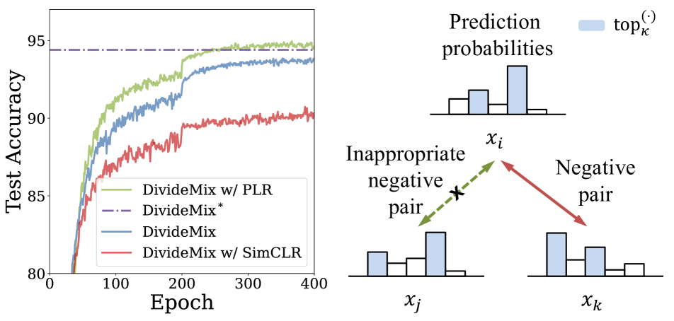
Figure 1: Left: Model performance suffers from trivially combining contrastive representation learning with supervised learning. The performance of DivideMix [28] (a supervised LNL method) boosts from using SimCLR [8] pretrained weights ($\mathrm{DivideMix}^{*}$), whereas suffers from being trivially combined with SimCLR contrastive loss ($\mathrm{DivideMix\ w/\ SimCLR}$). While DivideMix with our proposed PLR contrastive loss ($\mathrm{DivideMix\ w/\ PLR}$) achieves comparable results to $\mathrm{DivideMix}^{*}$. Right: Our proposed PLR contrastive loss selects a set of reliable negative pairs for each sample. The negative pair should have no overlap with the sample’s prediction probabilities at $\mathrm{top}_{\kappa}$ indices ($\kappa=2$ in Figure). As an instance, $x_{k}$ is a negative pair of $x_{i}$ as $\mathrm{top}_{2}^{(i)}\cap\mathrm{top}_{2}^{(k)}=\emptyset$, while $x_{j}$ is an inappropriate negative pair of $x_{i}$ as $\mathrm{top}_{2}^{(i)}\cap\mathrm{top}_{2}^{(j)}\neq\emptyset$.

Existing methods dealing with the so-called learning with noisy labels (LNL) problem can be mainly classified into two categories, namely label correction and sample selection. Label correction methods leverage the model predictions to correct noisy labels [40, 1]. Sample selection techniques attempt to divide samples with clean labels (usually with small losses) from noisy datasets [13, 19, 28]. Recent studies typically filter out the potentially noisy samples first, then apply label correction to those noisy samples, and finally train the model in a semi-supervised way [28].

Most label correction and sample selection methods take advantage of early learning phenomenon during the model training process [2]. Nevertheless, the intrinsic semantic information in data inherently resistant to label noise memorization has been disregarded in these methods [53]. The rapid development of self-supervised contrastive representation learning (CRL) methods [8, 16] shows new possibilities for modeling data representations without the requirements of data labels, which is beneficial for the model to correct corrupted labels or filter out noisy samples in datasets. Most recent studies either utilize the CRL to acquire robust pre-trained weights [44, 62, 12] or directly add the CRL loss to the total loss accompanying the supervised loss [20, 18].

While CRL helps models to learn representations without labels, a decrease in accuracy has been observed when it was trivially integrated with supervised losses (Figure 1 left). To address this issue, we propose the Pseudo-Label Relaxed (PLR) contrastive representation learning to avoid the conflict between supervised learning and CRL (Figure 1 right). Inappropriate negative pairs are removed by checking if their top $\kappa$ indices of prediction probabilities have an empty intersection. This results in a reliable negative set and will construct a more effective semantic clustering than vanilla CRL.

In addition to improving model robustness to noisy labels by utilizing CRL, we also design a new technique to filter out noisy samples based on inconsistencies between labels and semantics. Considering the semantic representation cluster formed by CRL, when the similarity between one sample’s projection embedding with its label prototype is smaller than that between itself and its cluster prototype, it may be given the wrong label. We adopt cross-entropy loss to formalize this sample selection method to obtain a consistent form with small loss selection techniques. Then, we dynamically fit a two-dimensional Gaussian Mixture Model (2d GMM) on the joint distribution of these two losses to divide clean and noisy samples.

Our main contributions are as follows:

• We analyze the conflict between supervised learning and CRL, attributing it to objective inconsistency and gradient conflicts. A novel PLR loss is proposed to alleviate this issue, facilitating our end-to-end PLReMix framework to enhance the capacity for LNL problems. Our proposed PLR loss can be easily integrated into other LNL methods and boost their performance as well.

• We propose a sample selection method based on the inconsistency between semantic representation clusters and labels. A 2d GMM is utilized to filter out noisy samples, considering both the early learning phenomenon of the model and intrinsic correlation in data.

• Extensive experiments on multiple benchmark datasets with varying types and label noise ratios demonstrate the effectiveness of our proposed method. We also conduct ablation studies and other analyses to verify the robustness of the components.

2 Related Work

2.1 Learning with noisy labels

Label correction. Label correction methods attempt to use the model predictions to correct the noisy labels. To this end, during training, a noise transition matrix is estimated to correct prediction by transforming noisy labels to their corresponding latent ground truth [9, 47]. Huang et al. [17] update the noisy labels with model predictions through the exponential moving average. P-correction [56] treats the latent ground truth labels as learnable parameters and utilizes back-propagation to update and correct noisy labels.

Sample selection. Sample selection techniques attempt to filter the samples with clean labels from a noisy dataset. Han et al. [13] select samples with small losses from one network as clean ones to teach the other. Dividemix [28] utilizes a two-component GMM to model the loss distribution to separate the dataset into a clean set and a noisy set. Sukhbaatar et al. [51] also consider the samples with consistent prediction and high confidence as clean samples.

Both label correction and sample selection methods benefit from the early learning phenomenon [31, 23, 2]. That is to say, the weights of DNNs will not stray far from the initial weights in the early stage of training [31]. Notably, several prior studies [23, 2, 46, 3] also observe the memorization effect in DNNs. This phenomenon demonstrates that DNNs tend to learn simple patterns and, over time, gradually overfit to more complex and noisy patterns.

2.2 Contrastive representation learning

CRL in self-supervised learning. CRL, a representative self-supervised learning technique, holds great promise in learning label-irrelevant representations. Basically, the main idea of self-supervised learning is to design a pretext task that allows models to learn pre-trained weights. CRL learns label-irrelevant representations of the model that identify positive and negative examples corresponding to a single sample from a batch of data. In SimCLR [8], two random augmentations are applied to each sample to obtain pairs of positive samples, while the other augmented samples are considered negative examples. A momentum encoder and a memory bank are adopted in MoCo [16] to generate and retrieve negative features of samples, which alleviates the high demand for large batch sizes.

CRL in learning with noisy labels. As a label-free method, CRL is resistant to noisy labels and can be beneficial for the LNL problem. Most of the recent studies follow a two or three-stage paradigm that uses CRL as a pretext task to obtain a pre-trained foundation model. Zheltonozhskii et al. [62] and Ghosh et al. [12] use CRL as a warmup method and outperform the fully-supervised pre-training on ImageNet. ScanMix [44] uses the CRL following a deep clustering method to pre-train the model, then jointly train the network with semi-supervised loss and clustering loss. Zhang et al. [60] utilizes CRL to pretrain the model, then trains a robust classification head on a fixed backbone, and finally trains in a semi-supervised way with a graph-structured regularization. We compare these frameworks in Figure 2 right.

A few methods have been proposed to address the complexity associated with pretrain fine-tuning pipeline of CRL within the overall LNL framework. Nevertheless, directly combining instance-wise CRL with supervised training objectives can interfere with the class-clustering ability, unlike forming clusters in a low-dimensional hypersphere surface in an unsupervised situation. In MoPro [29] and ProtoMix [30], the prototypical CRL that enforces the sample embedding to be similar to its assigned prototypes is jointly used with standard instance-wise CRL. MOIT [39] uses mixup interpolated supervised contrastive learning [21] to improve model robustness to label noise. UNICON [20] divides the dataset into clean and noisy sets, then trains in a semi-supervised manner with CRL loss applied on the noisy sets. Sel-CL+ [32] selects confident pairs by measuring the agreement between learned representations and labels to apply supervised contrastive learning to the LNL problem. Kim et al. [22] and Yan et al. [55] propose negative learning approaches to alleviate the impact of noisy labels by teaching the model to learn this is not something instead of this is something. Our method extends the self-supervised CRL by constructing a reliable negative set for each sample using pseudo-labels that the model predicts, thus alleviating the wrong contrast.

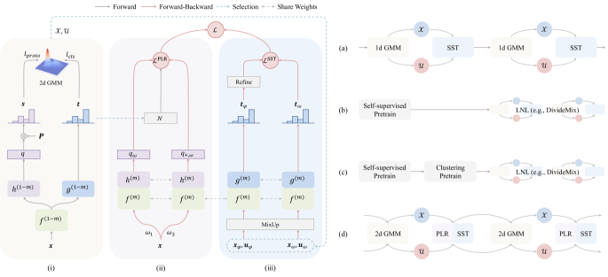
Figure 2: Left: Overview of the proposed method. (i) We perform joint sample selection on the first network to divide clean and noisy samples with 2d GMM. (ii) We train the second network with proposed Pseudo-Label Relaxed contrastive loss $\mathcal{L}^{\mathrm{PLR}}$ with the constructed reliable negative set $\mathcal{N}$ alleviating the conflict between the supervised learning and CRL. (iii) We utilize semi-supervised training for the second network on the clean and noisy samples divided by 2d GMM separately. The final learning objective $\mathcal{L}$ comprises two components, namely $\mathcal{L}^{\mathrm{PLR}}$ and $\mathcal{L}^{\mathrm{SST}}$. Right: Comparison of different LNL frameworks utilizing CRL. (a) DivideMix [28] iteratively performs sample selection (1d GMM) and semi-supervised training (SST). (b) The two-stage method [62, 12, 60] performs self-supervised pretraining before LNL. (c) The three-stage method [44] performs self-supervised pretraining and clustering pretraining before LNL. (d) By proposing PLR loss, our method unifies SST and CRL in an end-to-end PLReMix framework.

3 Proposed Method

3.1 Overview

The noisy dataset given in LNL is denoted as $\mathcal{D}=\{\boldsymbol{x}_{i},y_{i}\}_{i=1}^{N}$, where $\boldsymbol{x}_{i}$ represents a sample and $y_{i}$ is the corresponding label over $C$ classes, $N$ is the number of samples in the dataset. The presence of noisy samples causes label differences between the annotated labels $\{y_{i}\}^{N}_{i=1}$ and the ground truth labels $\{\tilde{y}_{i}\}^{N}_{i=1}$. Our proposed framework iteratively trains two identical networks, each consisting of a convolutional backbone $\boldsymbol{f}(\cdot;\theta^{(m)})$, a classification head $\boldsymbol{g}(\cdot;\phi^{(m)})$, and a projection head $\boldsymbol{h}(\cdot;\psi^{(m)})$. $m\in\{0,1\}$ denotes the network number. Given a minibatch of $b$ samples, the output logits of input $\boldsymbol{x}=\{\boldsymbol{x}_{i}\}_{i=1}^{b}$ are denoted as $\boldsymbol{z}=\boldsymbol{g}(\boldsymbol{f}(\boldsymbol{x};\theta^{(m)});\phi^{(m)})$, the output prediction probabilities are denoted as $\boldsymbol{t}=\mathrm{softmax}(\boldsymbol{z})$, the projection embeddings are denoted as $\boldsymbol{q}=\boldsymbol{h}(\boldsymbol{f}(\boldsymbol{x};\theta^{(m)});\psi^{(m)})$. We use a weak augmentation $\varphi$ and a strong augmentation $\omega$. Class prototypes $\boldsymbol{P}=\{\boldsymbol{p}_{k}\}_{k=1}^{C}$, are maintained and updated every epoch to represent the feature prototypes of the $k$-th class, where $\boldsymbol{p}_{k}\in\mathbb{R}^{d}$, $d$ is the dimension of projection embedding.

For the initialization of class prototypes $\boldsymbol{P}$ and initial model convergence, we warm up the two networks for a few epochs with cross-entropy loss and standard CRL loss on the whole dataset. At the end of the warmup, we initialize class prototypes by taking the average of feature embeddings with the same noisy labels. As shown in Figure 2 left, the proposed end-to-end LNL framework performs the following two steps iteratively in the training process: (1) divide the whole dataset into a clean and a noisy set considering their losses by a novel two-component 2d GMM (Section 3.2) and (2) train the other network with proposed Pseudo-Label Relaxed contrastive loss $\mathcal{L}^{\mathrm{PLR}}$ on the representations with a set of reliable negative pairs $\mathcal{N}_{i}$ for each sample (Section 3.3), and semi-supervised loss $\mathcal{L}^{\mathrm{SST}}$ on the divided clean and noisy sets (Section 3.4). $\mathcal{N}_{i}$ is denoted as $\mathcal{N}$ in Figure 2 left.

3.2 Joint sample selection

Sample selection We compute two cross-entropy losses $l_{i,cls}$ and $l_{i,proto}$ to fit a two-component 2d GMM for sample selection. First, following the small loss selection technique [13], we compute the cross-entropy classification loss $l_{i,cls}=-\log(\boldsymbol{t}_{i}^{y_{i}})$ to measure how well the model fits the pattern of a sample. Then, we define the class prototypes as the center of projection embeddings with similar semantics. The similarity between each projection embedding $\boldsymbol{q}_{i}$ and all the class prototypes $\{\boldsymbol{p}_{k}\}^{C}_{k=1}$ represents the latent class probability distributions at the semantic level. Following MoPro [29], we use softmax normalized cosine similarity to measure the similarity between $\boldsymbol{q}_{i}$ and $\boldsymbol{p}_{k}$:

$$\boldsymbol{s}_{i}=\{s_{i}^{k}\}_{k=1}^{C}=\left\{\frac{\exp{(\boldsymbol{q}_{i}\cdot\boldsymbol{p}_{k}/\tau_{s})}}{\sum_{k=1}^{C}\exp{(\boldsymbol{q}_{i}\cdot\boldsymbol{p}_{k}/\tau_{s})}}\right\}_{k=1}^{C},\vspace{-0.3em}$$ (1)

where sharpen temperature $\tau_{s}$ is $0.1$ in this paper. Projection embeddings for the samples with similar semantics tend to form clusters around corresponding prototypes under the effect of CRL. In such a case, if a sample $\boldsymbol{x}_{i}$ is mislabeled to $y_{i}$, we suppose to have $s_{i}^{y_{i}}<s_{i}^{\tilde{y}_{i}}$, where $\tilde{y}_{i}$ is the latent ground truth class of $\boldsymbol{x}_{i}$. Based on the above discussion, the distance between the distribution of $\boldsymbol{s}_{i}$ and OneHot$(y_{i})$ is supposed to be smaller for clean samples than for noisy samples. Thus, we can compute another cross-entropy loss $l_{i,proto}=-\log(\boldsymbol{s}_{i}^{y_{i}})$ to measure if the given label matches the semantic cluster.

After obtaining the $l_{i,cls}$ and the $l_{i,proto}$ for all samples, a two-component 2d GMM on the distribution of $\boldsymbol{l}=\{\boldsymbol{l}_{i}\}_{i=1}^{N}=\{(l_{i,cls},l_{i,proto})\}_{i=1}^{N}$ can be computed. Suppose the two Gaussian components are $\boldsymbol{G_{1}}(\cdot;\boldsymbol{\mu}_{1},\boldsymbol{\Sigma}_{1})$ and $\boldsymbol{G_{2}}(\cdot;\boldsymbol{\mu}_{2},\boldsymbol{\Sigma}_{2})$, we obtain the probability $w_{i}$ of each sample to be clean from posterior probability as:

$$w_{i}=p\left(\boldsymbol{G}_{j}\mid\boldsymbol{l}_{i}\right)\quad\mathrm{with}\quad j={\mathop{\arg\min}\limits_{j\in\{1,2\}}\left\|\boldsymbol{\mu}_{j}\right\|_{2}}.\vspace{-0.5em}$$ (2)

Samples predicted have smaller $\left\|\boldsymbol{\mu}_{j}\right\|_{2}$ are considered as clean samples, which form the clean set denoted by $\mathcal{X}$. While the remaining samples are considered as noisy and form the noisy set $\mathcal{U}$.

Momentum class prototypes We adopt noise correction and exponential moving average (EMA) to update the class prototypes $\{\boldsymbol{p}_{k}\}^{C}_{k=1}$ while training. Due to the slow convergence speed of CRL, its projection embeddings $\boldsymbol{q}_{i}$ are not optimal and robust in the early epochs, thus resulting in inaccurate $\boldsymbol{s}_{i}$ in Eq. (1). To better estimate the latent ground truth label $\tilde{y}_{i}$, we generate a pseudo soft label $\boldsymbol{\delta}_{i}=\alpha\boldsymbol{t}_{i}+(1-\alpha)\boldsymbol{s}_{i}$ for $\boldsymbol{x}_{i}$ considering both model predictions and semantic cluster. Accordingly, noise correction and sample selection are performed to set a correction threshold $\tau_{1}$ and a high prediction confidence threshold $\tau_{2}$, i.e.

$$\hat{y}_{i}=\left\{\begin{array}[]{lcl}\mathop{\arg\max}\limits_{c\in C}\boldsymbol{\delta}_{i}^{c}&&\mathrm{if}\ \mathop{\max}\limits_{c\in C}\boldsymbol{\delta}_{i}^{c}>\tau_{1},\\ y_{i}&&\mathrm{elseif}\ \mathop{\max}\boldsymbol{\delta}_{i}^{y_{i}}>\tau_{2},\\ \mathrm{unknown}&&\mathrm{otherwise}.\\ \end{array}\right.$$ (3)

The selected high prediction confidence samples $\{\boldsymbol{x}_{i}\mid i\ \neq\ \mathrm{unknown}\}$ constitute the confident set denoted as $\mathcal{C}$. With the estimated labels, we update the projection embedding $\boldsymbol{q}_{i}$ to the corresponding class prototype $\boldsymbol{p}_{\hat{y}_{i}}$ using EMA:

$$\boldsymbol{p}_{\hat{y}_{i}}\leftarrow\mathrm{Normalize}\left(\eta\boldsymbol{p}_{\hat{y}_{i}}+(1-\eta)\mathrm{Normalize}(\boldsymbol{q}_{i})\right),\\$$ (4)

for all ${\{\boldsymbol{x}_{i},\hat{y}_{i}\}}\in\mathcal{C}$, where $\mathrm{Normalize}(\boldsymbol{x})=\boldsymbol{x}/\left\|\boldsymbol{x}\right\|_{2}$ and the momentum coefficient $\eta$ is set to $0.99$.

3.3 Pseudo-Label Relaxed contrastive representation learning

Typically, unsupervised CRL methods use two transforms of a single sample as a positive pair and combinations of transforms of other samples as negative pairs. We intend to design a loss function that will bring positive pairs together and push negative pairs apart. Specifically, the vanilla InfoNCE loss for the embedding $\boldsymbol{q}_{i,\omega}$ of an augmented sample used in CPC [38] and SimCLR [8] are defined as:

$$-\sum_{i=1}^{N}\log\frac{\exp\left(\left\langle\boldsymbol{q}_{i,\omega},\boldsymbol{q}_{+,\omega}\right\rangle/\tau\right)}{\displaystyle\begin{multlined}\exp\left(\left\langle\boldsymbol{q}_{i,\omega},\boldsymbol{q}_{+,\omega}\right\rangle/\tau\right)+\\ \sum_{\boldsymbol{q}_{j,\omega}\in\{\boldsymbol{q}_{-,\omega}\}}\exp\left(\left\langle\boldsymbol{q}_{i,\omega},\boldsymbol{q}_{j,\omega}\right\rangle/\tau\right)\end{multlined}\exp\left(\left\langle\boldsymbol{q}_{i,\omega},\boldsymbol{q}_{+,\omega}\right\rangle/\tau\right)+\\ \sum_{\boldsymbol{q}_{j,\omega}\in\{\boldsymbol{q}_{-,\omega}\}}\exp\left(\left\langle\boldsymbol{q}_{i,\omega},\boldsymbol{q}_{j,\omega}\right\rangle/\tau\right)},\vspace{-0.5em}$$ (5)

where $\tau$ is the sharpening temperature. $\{\boldsymbol{q}_{+,\omega}\}$ and $\{\boldsymbol{q}_{-,\omega}\}$ are the projection embeddings of augmented positive and negative samples, respectively, $\left\langle\boldsymbol{a},\boldsymbol{b}\right\rangle$ represents cosine similarity $\mathrm{Normalize}\left(\boldsymbol{a}\cdot\boldsymbol{b}\right)$. We note that there exist some negative embeddings $\boldsymbol{q}_{j,\omega}\in\{\boldsymbol{q}_{-,\omega}\}$ whose ground truth labels are identical to the positive embedding $\boldsymbol{q}_{i,\omega}$. These samples will also be pushed away from $\boldsymbol{q}_{i,\omega}$ with the use of the term $\exp\left(\left\langle\boldsymbol{q}_{i,\omega},\boldsymbol{q}_{j,\omega}\right\rangle/\tau\right)$ in Eq. (5), which conflicts with the design purpose of other supervised losses used in LNL problems. Worse still, this effect is exacerbated when the $i$-th sample and $j$-th sample are more similar, resulting in a more dispersed cluster.

We proposed the PLR loss to address this issue, which is robust to both clean and noisy samples. A reliable negative set $\mathcal{N}_{i}$ is designed to remove the samples in $\{\boldsymbol{q}_{-,\omega}\}$ that share the same latent ground truth with $\boldsymbol{q}_{i,\omega}$. To this end, given a prediction probability $\boldsymbol{t}_{i}=\left[t_{i,1},t_{i,2},\ldots,t_{i,C}\right]$, we first identify the indexes of the top $\kappa$ digits of the prediction probability $\boldsymbol{t}_{i}$ of the $i$-th sample, which is denoted by $\mathrm{top}_{\kappa}^{(i)}$:

$$\mathrm{top}_{\kappa}^{(i)}=\mathop{\arg\max}\limits_{\kappa}\{t_{i,\kappa}\}^{C}_{\kappa=1}.\vspace{-0.5em}$$ (6)

Thus, the reliable negative set of $\boldsymbol{x}_{i}$ can be obtained as:

$$\left\{j\mid{\mathrm{top}_{\kappa}^{(i)}}\cap{\mathrm{top}_{\kappa}^{(j)}}=\emptyset,\forall j\right\}.\vspace{-0.5em}$$ (7)

During the early training stage, we additionally append the given label $y_{i}$ to the top${}_{\kappa}^{(i)}$ for further conflict avoidance:

$$\mathcal{N}_{i}=\left\{j\mid\{\mathrm{top}_{\kappa}^{(i)}\cup y_{i}\}\cap\{\mathrm{top}_{\kappa}^{(j)}\cup y_{j}\}=\emptyset,\forall j\right\}.\vspace{-0.5em}$$ (8)

Finally, the proposed PLR loss is re-formulated based on the vanilla InfoNCE loss of Eq. (5) to the following expression:

$$\mathcal{L}^{\mathrm{PLR}}=-\sum_{i=1}^{N}\log\frac{\exp\left(\left\langle\boldsymbol{q}_{i,\omega},\boldsymbol{q}_{+,\omega}\right\rangle/\tau\right)}{\displaystyle\begin{multlined}\exp\left(\left\langle\boldsymbol{q}_{i,\omega},\boldsymbol{q}_{+,\omega}\right\rangle/\tau\right)+\\ \sum_{j\in\mathcal{N}_{i}}\exp\left(\left\langle\boldsymbol{q}_{i,\omega},\boldsymbol{q}_{j,\omega}\right\rangle/\tau\right)\end{multlined}\exp\left(\left\langle\boldsymbol{q}_{i,\omega},\boldsymbol{q}_{+,\omega}\right\rangle/\tau\right)+\\ \sum_{j\in\mathcal{N}_{i}}\exp\left(\left\langle\boldsymbol{q}_{i,\omega},\boldsymbol{q}_{j,\omega}\right\rangle/\tau\right)}.\vspace{-0.3em}$$ (9)

We use two forms of PLR loss in this paper: the FlatNCE [7] formalized PLR loss is denoted as FlatPLR, while the InfoNCE formalized one is denoted just as PLR. We do experiments on gradient analysis between $\mathcal{L}^{\mathrm{PLR}}$ and $\mathcal{L}^{\mathrm{CRL}}$ in Section 4.4, whose results show that $\mathcal{L}^{\mathrm{PLR}}$ has less gradient conflicts with the supervised loss.

3.4 Semi-supervised training

As described in Section 3.2, according to the proposed sample selection technique, we divide the noisy dataset $\mathcal{D}$ into a labeled set $\mathcal{X}$ and an unlabeled set $\mathcal{U}$ using 2d GMM. Then, we perform semi-supervised training on them following FixMatch [45] and MixMatch [4].

First, we generate pseudo targets $\overline{\boldsymbol{y}}_{i}$ for each sample using weak augmentations:

$$\leavevmode\resizebox{469.75499pt}{}{$\begin{cases}\operatorname{Sharpen}\left(w_{i}\operatorname{OneHot}\left(y_{i}\right)+\frac{1-w_{i}}{\operatorname{card}(\varphi)}\sum_{\varphi}\boldsymbol{t}_{i,\varphi};T\right),\text{ if }\boldsymbol{x}_{i}\in\mathcal{X},\\ \operatorname{Sharpen}\left(\frac{1}{\operatorname{card}(\varphi)\operatorname{card}(m)}\sum_{\varphi,m}\boldsymbol{t}_{i,\varphi}^{m};T\right),\text{ if }\boldsymbol{x}_{i}\in\mathcal{U},\end{cases}$}\vspace{-1.5em}$$ (10)

and

$$\mathrm{Sharpen}(\bar{\boldsymbol{y}}_{i};T)={\bar{\boldsymbol{y}}_{i}^{c\frac{1}{T}}}/\sum_{c=1}^{C}{\bar{\boldsymbol{y}}_{i}^{c\frac{1}{T}}},\ \mathrm{for}\ c=1,2,...,C,\vspace{-0.5em}$$ (11)

where ${\mathrm{card}}(\varphi)$ and ${\mathrm{card}}(m)$ represent the numbers of augmentations and models, respectively, and the sharpening temperature $T$ is $0.5$. Then we do MixUp [61] on the strong augmented samples $\boldsymbol{x}_{i,\omega}$ and pseudo targets $\bar{\boldsymbol{y}}_{i}$:

$$\boldsymbol{x}_{i,\omega}^{\prime} =\lambda\boldsymbol{x}_{i,\omega}+(1-\lambda)\boldsymbol{x}_{r(i),\omega},$$ (12)

$$\bar{\boldsymbol{y}}_{i}^{\prime} =\lambda\bar{\boldsymbol{y}}_{i}+(1-\lambda)\bar{\boldsymbol{y}}_{r(i)},$$

where $\lambda\sim\mathrm{Beta}(\beta,\beta)$, $r(i)$ represents the random permutation of indices $i$. Finally, the semi-supervised loss $\mathcal{L}^{\mathrm{SST}}$ consists of three parts: a cross-entropy loss on the labeled set, a mean squared error on the unlabeled set, and a regularization term $\mathcal{L}_{reg}$ used in [49] and [1]:

$$\mathcal{L}^{\mathrm{SST}}=-\frac{1}{|\mathcal{X}|}\sum_{\boldsymbol{x}_{i}\in\mathcal{X}}\sum_{c=1}^{C}\bar{\boldsymbol{y}}_{i}^{\prime c}\log(\boldsymbol{t}_{i,\omega}^{\prime c})+\\ \lambda_{\mathcal{U}}\frac{1}{|\mathcal{U}|}\sum_{\boldsymbol{x}_{i}\in\mathcal{U}}\left\|\bar{\boldsymbol{y}}_{i}^{\prime}-\boldsymbol{t}_{i,\omega}^{\prime}\right\|_{2}^{2}+\mathcal{L}_{\mathrm{reg}},\vspace{-1em}$$ (13)

where $\lambda_{\mathcal{U}}$ is a coefficient for tuning. The final objective objective $\mathcal{L}$ is to minimize the following function:

$$\mathcal{L}=\mathcal{L}^{\mathrm{SST}}+\lambda_{i}\mathcal{L}^{\mathrm{PLR}},\vspace{-0.5em}$$ (14)

where $\lambda_{i}$ is a tunable hyperparameter.

4 Experiments

Table 1: Experimental and comparison results on CIFAR-10 and CIFAR-100 datasets with different noise ratios (test accuracy %).

Method Dataset CIFAR-10 CIFAR-100 Mode Sym Asym Sym Asym $r$ 20% 50% 80% 90% 40% 20% 50% 80% 90% 40% Cross-entropy Best 86.8 79.4 62.9 42.7 85.0 62.0 46.7 19.9 10.1 44.5 Last 82.7 57.9 26.1 16.8 72.3 61.8 37.3 8.8 3.5 - Co-teaching+ [58] Best 89.5 85.7 67.4 47.9 - 65.6 51.8 27.9 13.7 - Last 88.2 84.1 45.5 30.1 - 64.1 45.3 15.5 8.8 - MixUp [61] Best 95.6 87.1 71.6 52.2 - 67.8 57.3 30.8 14.6 48.1 Last 92.3 77.3 46.7 43.9 77.7 66.0 46.6 17.6 8.1 - DivideMix [28] Best 96.1 94.6 93.2 76.0 93.4 77.3 74.6 60.2 31.5 55.1 Last 95.7 94.4 92.9 75.4 92.1 76.9 74.2 59.6 31.0 - ScanMix [44] Best 96.0 94.5 93.5 91.0 93.7 77.0 75.7 66.0 58.5 - Last 95.7 93.9 92.6 90.3 93.4 76.0 75.4 65.0 58.2 - MOIT+ [39] Best 94.1 91.8 81.1 74.7 93.3 75.9 70.6 47.6 41.8 74.0 Sel-CL+ [32] Best 95.5 93.9 89.2 81.9 93.4 76.5 72.4 59.6 48.8 72.7 ELR+ [34] Best 95.8 94.8 93.3 78.7 93.3 77.6 73.6 60.8 33.4 73.2 UNICON [20] Best 96.0 95.6 93.9 90.8 94.1 78.9 77.6 63.9 44.8 74.8 (Flat) PLReMix Best 96.63 95.71 95.08 91.93 95.11 77.95 77.78 68.76 50.17 64.89 Last 96.46 95.36 94.84 91.54 94.72 77.78 77.31 68.41 49.44 62.67

4.1 Experimental settings

CIFAR10/100 The CIFAR10/100 dataset [24] comprises 50K training images and 10K test images. We adopt symmetric and asymmetric synthetic label noise models as used in previous studies [49]. The symmetric noise setting replaces $r\%$ of labels from one class uniformly with all possible classes, while asymmetric replaces them from one class only with the most similar class.

We use the PreAct ResNet-18 [15] network on CIFAR 10/100 and train it using an SGD optimizer. To avoid conflict early and gain robust representation later, we reduce $\kappa$ from $3$ to $2$ to $1$ at the epochs of 40 and 70. In this work, we use AutoAug [10] as a strong augmentation operation, which is demonstrated to be useful in the LNL problem [37]. We use FlatPLR for CIFAR experiments to gain a greater thrust between samples and their negative pairs with a relatively small batch size. For more training details, please refer to the Appendix.

Tiny-ImageNet Tiny-ImageNet [27] consists of 200 classes, each containing 500 smaller-resolution images from ImageNet. We train a PreAct ResNet 18 [15] network with a batch size of 128 and a learning rate of 0.01.

Clothing1M Clothing1M [54], a large-scale real-world dataset with label noise, contains 1M clothing images from 14 classes. We sample 64K images in total from each class [28]. We train a ResNet50 network with weights pre-trained on ImageNet [14] for 100 epochs.

WebVision WebVision dataset [33] contains 2.4 M images crawled from Flickr and Google. All of the images are categorized into 1,000 classes, which is the same as ImageNet ILSVRC12 [43]. We use the first 50 classes of the Google image subset to train an InceptionResnet V2 [48] from scratch. Multi-crop augmentation strategy [5] is exploited to obtain more robust representations in rather shorter epochs and smaller batch size so that contrastive loss can be jointly trained with the semi-supervised loss. See the Appendix for more details about multi-crop.

Table 2: Experimental and comparison results on Tiny-ImageNet dataset (test accuracy %).

Method $r$ Sym Asym 0 20% 50% 80% 45% Cross-entropy Best 57.4 35.8 19.8 - 26.3 Last 56.7 35.6 19.6 - 26.2 Co-teaching+ [58] Best 52.4 48.2 41.8 - 26.9 Last 52.1 47.7 41.2 - 26.5 M-correction [1] Best 57.7 57.2 51.6 - 24.8 Last 57.2 56.6 51.3 - 24.1 UNICON [20] Best 63.1 59.2 52.7 - - Last 62.7 58.4 52.4 - - (Flat) PLReMix Best 62.93 60.70 54.94 37.47 33.97 Last 62.46 60.39 54.31 36.43 33.25

Method Test Accuracy Cross-Entropy 69.21 Joint-Optim [49] 72.16 P-correction [56] 73.49 DivideMix [28] 74.76 ELR+ [34] 74.81 UNICON [20] 74.98 C2D [62] 74.30 ScanMix [44] 74.35 PLReMix 74.85

Table 3: Experimental and comparison results on Clothing1M dataset (test accuracy %).

4.2 Experimental results

The proposed end-to-end PLReMix framework is compared with other LNL methods on different datasets using the same network architecture. The experimental results on CIFAR10/100 are shown in Table 1. We report the best test accuracy over all epochs and the average test accuracy of the last 10 epochs as Best and Last, respectively. Considering the intrinsic semantic features by utilizing PLR loss and 2d GMM, our proposed method outperforms state-of-the-art (SOTA) results in most experimental settings, especially on data with high noise ratios. We attribute our inferior results to SOTA on CIFAR100 with 40% asymmetric noise to worse initialization of class prototypes across too many classes, and the absence of a uniform sample selection technique proved to be useful [20]. However, our method still outperforms the baseline method [28] a lot.

The experimental results on Tiny-ImageNet are shown in Table 2. Our algorithm achieves SOTA performance on most noise ratios. The results of the real-world noisy dataset Clothing1M are shown in Table 3, and the results of the WebVision dataset are listed in Table 4. Our algorithm achieves performance comparable to SOTA. It is notable that C2D [62] and ScanMix [44] use pretrained weights in a two/three-stage manner. As a comparison, our proposed method trains the model end-to-end with randomly initialized weights.

Table 4: Experimental and comparison results on WebVision and ILSVRC12 datasets (test accuracy %). Models are trained on the WebVision dataset and tested on both the WebVision and ILSVRC12 datasets. Top-1 and Top-5 test accuracy are reported.

Dataset Architecture WebVision ILSVRC12 Method Top-1 Top-5 Top-1 Top-5 Co-Teaching [13] Inception V2 63.58 85.20 61.48 84.70 DivideMix [28] Inception V2 77.32 91.64 75.20 90.84 ELR+ [34] Inception V2 77.78 91.68 70.29 89.76 UNICON [20] Inception V2 77.60 93.44 75.29 93.72 Sel-CL+ [32] Inception V2 79.96 92.64 76.84 93.04 ScanMix [44] Inception V2 80.04 93.04 75.76 92.60 PLReMix Inception V2 80.19 93.51 75.82 93.16

4.3 Scalability of PLR

We do extra experiments on the CIFAR10 dataset with other different LNL algorithms to demonstrate the effectiveness and scalability of our proposed PLR loss. We integrate our proposed PLR loss into Co-teaching+ [58] and JoCoR [52] and test the model performance under different noise ratios. We use PreAct ResNet18 network, and the minor modification to the original algorithms is just training a projection head using our proposed PLR loss on top of the model backbone. As a comparison, we utilize the vanilla SimCLR to train the projection head. The experimental results are listed in Table 5. As can be seen, training with our proposed PLR increases the model performance compared to the baseline methods, while training with vanilla SimCLR tends to make the model performance corrupted. These results align with our analysis of the gradient conflicts in Section 4.4.

Method CRL CIFAR-10 Sym-20% Sym-50% Asym-40% Co-teaching+ [58] - 88.73 77.52 68.64 SimCLR 88.62 80.24 68.86 PLR 90.28 85.68 70.92 JoCoR [52] - 88.13 80.94 75.48 SimCLR 84.76 78.81 78.56 PLR 89.34 83.46 81.46

Table 5: Experimental results of combining different CRL methods with LNL algorithms (test accuracy %).

4.4 Analysis

Multi-task gradients. Given two losses $\mathcal{L}^{\left(1\right)}$ and $\mathcal{L}^{\left(2\right)}$ and their gradients to model parameters $\boldsymbol{g}^{\left(1\right)}$ and $\boldsymbol{g}^{\left(2\right)}$, we define the intensity of gradient entanglement between them as $\mathcal{E}^{\left(1\right)}_{\left(2\right)}=\boldsymbol{g}^{\left(1\right)}\cdot\boldsymbol{g}^{\left(2\right)}/{\left\|\boldsymbol{g}^{\left(2\right)}\right\|}_{2}^{2}$, the ratio of gradient magnitude between them as $\mathcal{R}^{\left(1\right)}_{\left(2\right)}={\left\|\boldsymbol{g}^{\left(1\right)}\right\|}_{2}/{\left\|\boldsymbol{g}^{\left(2\right)}\right\|}_{2}$.

Conflicting gradients and a large difference in gradient magnitudes often lead to optimization challenges in high-dimensional neural network multi-task learning [57]. Similar issues are witnessed in our experiments. Here, $\mathcal{L}^{\mathrm{SimCLR}}$ or $\mathcal{L}^{\mathrm{PLR}}$ is treated as $\mathcal{L}^{\left(1\right)}$, $\mathcal{L}^{\mathrm{SST}}$ is treated as $\mathcal{L}^{\left(2\right)}$. As shown in Figure 3, we show the distribution of $\mathcal{E}^{\mathrm{SimCLR}}_{\mathrm{SST}}$ and $\mathcal{E}^{\mathrm{PLR}}_{\mathrm{SST}}$ (Left), $\mathcal{R}^{\mathrm{SimCLR}}_{\mathrm{SST}}$ and $\mathcal{R}^{\mathrm{PLR}}_{\mathrm{SST}}$ (Right) when training models on CIFAR10 dataset with 80% noise ratio at epoch 30.

The entanglement intensity between SimCLR and SST shows more negative values, and their magnitude ratio has more values greater than 1. These indicate that there are more gradient conflicts between $\mathcal{L}^{\mathrm{SST}}$ and $\mathcal{L}^{\mathrm{SimCLR}}$, which result in an optimization challenge and performance decrease shown in Figure 1 left red line. Our proposed PLR loss mitigates the gradient conflicts with SST, which manifests as more orthogonal gradients and smaller gradient magnitude ratios. As a result, it improves the performance when integrated with SST to combat noisy labels, as shown in Figure 1 left green line.

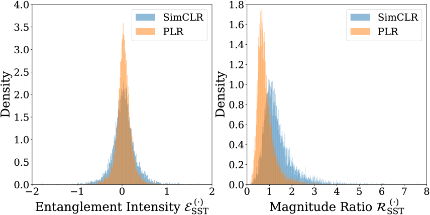
Figure 3: Gradient conflicts of two contrastive representation learning methods (vanilla SimCLR and our proposed PLR) when they are jointly trained with semi-supervised learning in the presence of noisy labels.

Ablation study. We perform thorough ablation studies on our method. The results of ablation studies are shown in Table 6. We test the effectiveness of FlatNCE by swapping it with (non-Flat) PLR, which is formalized by InfoNCE loss. Despite using InfoNCE instead of FlatNCE, our experiments still show the robustness of the proposed PLR loss. Then, we substitute the PLR loss with vanilla SimCLR [8]. Experiments where 2d GMM is replaced with 1d GMM confirm that semantic information helps differentiate clean and noisy samples on the distribution of $\boldsymbol{l}=\{(l_{i,cls})\}_{i=1}^{N}$. Supervised contrastive loss (SCL) [21] treats samples with the same labels as positive pairs, and others are negative pairs. It can be a substitute for our proposed PLR loss in our framework when it considers samples with the same predicted pseudo labels as positive pairs. We do experiments to compare SCL and PLR in our proposed framework. The results show that our proposed PLR outperforms SCL in most noise ratios except on the CIFAR100 dataset with a high noise ratio.

Table 6: Ablation studies on CIFAR-10 and CIFAR-100 datasets with different training settings (test accuracy %).

Method Dataset CIFAR-10 CIFAR-100 $r$ 50% 80% 90% 50% 80% 90% (Flat) PLReMix Best 95.71 95.08 91.93 77.78 68.76 50.17 Last 95.36 94.84 91.54 77.31 68.41 49.44 PLReMix Best 95.71 93.58 91.71 75.64 66.98 50.78 Last 95.31 93.39 91.46 75.39 66.76 50.54 vanilla SimCLR Best 93.44 90.44 86.80 73.10 63.50 47.76 Last 93.23 90.28 86.51 72.32 63.02 46.81 (Flat) 1d GMM Best 94.51 94.82 92.36 77.11 68.54 50.25 Last 94.16 94.57 92.12 76.91 68.31 49.99 SCL Best 94.37 93.41 91.24 72.55 68.43 54.07 Last 94.08 93.11 91.00 72.18 68.03 53.72

Table 7: Ablation study results when using different $\kappa$ or only given labels on CIFAR10 dataset with 80% symmetric label noise.

$\kappa=3$ $\kappa=2$ $\kappa=1$ only $y$ PLReMix Best 91.83 93.93 93.74 94.74 95.08 Last 91.29 92.81 93.60 94.58 94.84

We conduct ablation experiments on the hyperparameter $\kappa$. Intuitively, larger values of $\kappa$ avoid conflict between PLR and supervised loss more effectively but result in less robust representation due to insufficient negative pairs. To address this issue, we decrease $\kappa$ from 3 to 2 to 1 after training a certain number of epochs. The decrease epochs are not carefully tuned and are set roughly evenly. In this ablation study, we fix the value of $\kappa$ as 3, 2, or 1 during different individual training procedures. In addition, we test the performance only using the given labels (denoted by only $y$), which means $\mathcal{N}_{i}=\left\{j\mid y_{i}\cap y_{j}=\emptyset,\forall j\right\}$. The experiments are conducted on the CIFAR10 dataset with 80% symmetric noise, and the results are listed in Table 7. The experimental results verify our analysis and show the effectiveness of the proposed decrease setting.

Visualization. We visualize the 2d GMM after 10 epochs of warming up and 100 epochs of training in Figure 4. We plot the losses of 512 randomly selected samples, with half from the clean set and the other half from the noisy set. As illustrated, our proposed 2d GMM effectively fits the distribution of the clean and noisy samples.

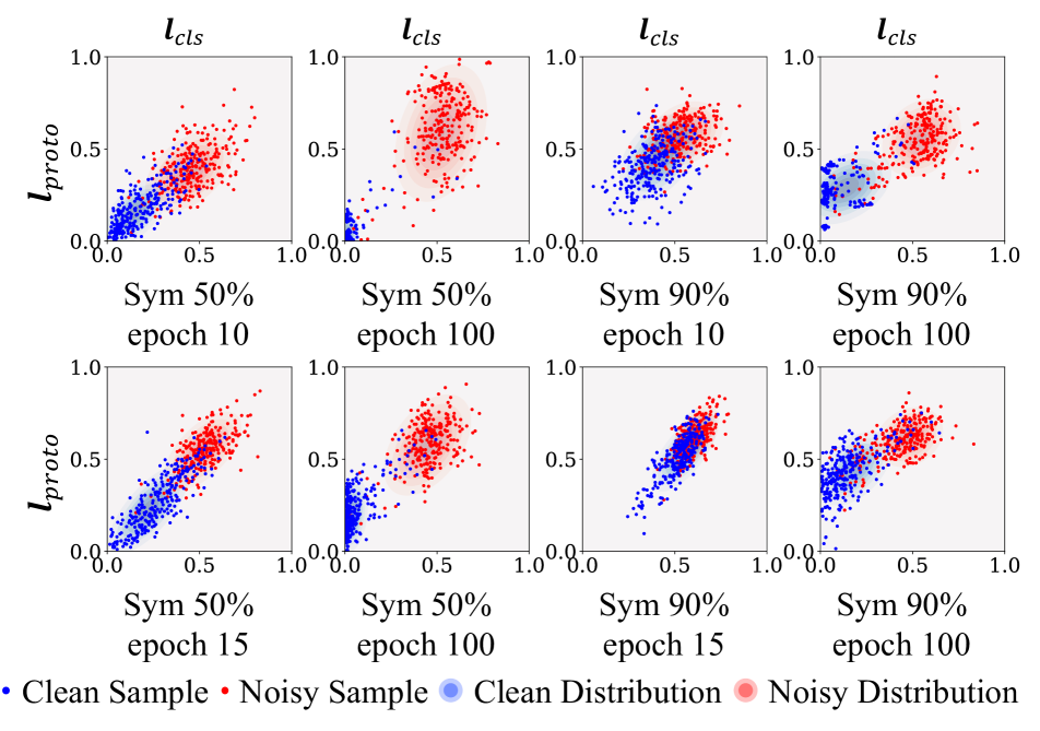
Figure 4: Visualization of the 2d GMM fitted on the normalized loss distribution $\left\{\left(\boldsymbol{l}_{cls},\boldsymbol{l}_{proto}\right)\right\}$. The first and second rows are obtained from experiments on the CIFAR10 and CIFAR100, respectively.

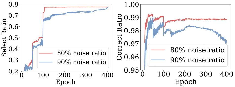
Figure 5: Negative sample selection when training with FlatPLR. Left: Negative pairs selected ratio. Right: Correct negative pairs selected ratio.

Correct ratio of negative pairs. We visualize the correct ratio of selected negative pairs in Figure 5 for a better understanding of the proposed PLR loss. The select ratio is the proportion of selected negative sample pairs out of all possible negative sample pairs. The correct ratio represents the proportion of correctly identified negative pairs among all selected pairs. We observed that the PLR loss tends to select a limited number of negative pairs at first to ensure high precision. As $\kappa$ gradually decreases, PLR loss will rapidly increase the number of negative sample pairs selected while maintaining precision.

5 Conclusion and Future Work

In this work, we proposed an end-to-end framework for solving the LNL problem by leveraging CRL. We analyzed conflicts between CRL learning objectives and supervised ones and proposed PLR loss to address this issue in a simple yet effective way. For further utilizing label-irrelevant intrinsic semantic information, we propose a joint sample selection technique, which expands previously widely used 1d GMM to 2d. Extensive experiments conducted on benchmark datasets show performance improvements of our method over existing methods. Our end-to-end framework shows significant improvement without any complicated pretrain fine-tuning pipeline. Future research should also explore other forms of PLR loss, such as MoCo-based.

Supplementary Material

A Pseudocode of Pseudo-Label Relaxed loss

Algorithm 1 provides the pseudocode of our proposed PLR loss. For a mini-batch of samples $\boldsymbol{x}$, we first calculate their model prediction probabilities using the first network. Based on the predicted probabilities, we then determine if there are overlapping top_κ predictions denoted as conflicts and use it to identify feasible negative samples. The reliable negative set $\mathcal{N}_{i}$ for each sample is built in the form of a contrastive mask, indicating which pairs are negative, positive, or neglected when conducting CRL. Finally, we transform the samples $\boldsymbol{x}$ into two strong augmented views, which are then utilized to train a contrastive loss (using the mask to identify the positive and reliable negative pairs) on the other network.

Algorithm 1 Pseudocode of computing PLR loss in a PyTorch-like style.

⬇

# net0, net1: two identical networks with backbone f, classification head g, and projection head h

# PLRLoss: contrastive loss, Eqn.(9), which takes a mask as parameter

# k: hyperparameter kappa in Eqn.(6)

def build_mask(x, y, net):

z = net.g.forward(net.f.forward(x)) # model outputs

indices_k = torch.topk(z, k, dim=1)[1] # top k indices of model outputs

# tops: assign 1 to the top k indices, 0 to the rest

tops = torch.zeros(len(x), C)

tops = torch.scatter(tops, 1, indices_k, 1)

tops = torch.scatter(tops, 1, y.unsqueeze(1), 1) # append labels to top k

# intersection, Eqn.(8), where ‘conflicts’ equals 0 are feasible negative pairs

conflicts = torch.matmul(tops, tops.t())

# contrastive mask, where negative pairs are -1, positive pairs are 1, neglect pairs are 0

mask = torch.where(conflicts == 0, -1, 0)

mask = torch.where(eye(len(x)) == 1, 1, mask)

return mask

for (x, y) in loader: # load a minibatch of samples and labels

mask = build_mask(x, y, net0) # get mask from one network

x1 = aug(x) # random strong augmentation

x2 = aug(x) # another strong augmentation

# train the other network

f1 = net1.h.forward(net1.f.forward(x1))

f2 = net1.h.forward(net1.f.forward(x2))

f = torch.cat([f1.unsqueeze(1), f2.unsqueeze(1)], dim=1)

plr_loss = InfoNCELoss()(f, mask=mask)

# if other losses exist, sum all losses up, then backward and update

plr_loss.backward()

update(net1.params) # train the other network

B Training Details

CIFAR10/100 We use the PreAct ResNet-18 [15] network on CIFAR 10/100 and train it using an SGD optimizer with a weight decay of 5e-4, a momentum of 0.9, and a batch size of 64. We choose $\lambda_{\mathcal{U}}$ from $\{0,25,50,150\}$ following the previous work [28], although experiments show that our method is not sensitive to this parameter. We set the initial learning rate to 0.02 and reduce it by a factor of 10 after 200 epochs. The warmup period is 10 for CIFAR10 and 15 for CIFAR100. We use the Flat version of the proposed PLR loss on these two datasets. To avoid conflict early and gain robust representation later, we reduce $\kappa$ from $3$ to $2$ to $1$ at the epochs of 40 and 70. We empirically set $\tau_{1}=0.5$ for $\mathcal{X}$, especially when the label noise is asymmetric; otherwise, set $\tau_{1}=1/C$.

Tiny-ImageNet We train a PreAct ResNet 18 [15] network with an SGD optimizer and a batch size of 128. We set the initial learning rate to 0.01 and reduce it by a factor of 10 after 200 epochs. $\lambda_{\mathcal{U}}$ is chosen from $\{0,25,50,150\}$ and $\beta$ is $0.5$. We use the Flat version of the proposed PLR loss on this dataset, and $\kappa$ is reduced at the epochs of 40 and 70.

Clothing1M We train a ResNet50 network with weights pre-trained on ImageNet [14] for 80 epochs with a learning rate of 5e-3, a weight decay of 1e-3, and a batch size of 64. We use $\lambda_{\mathcal{U}}=0$ and $\beta=0.5$ on the Clothing1M dataset. The network is trained for 100 epochs with a warmup period of 1 epoch. We reduce $\kappa$ at the epochs of 15 and 30. We fix the backbone parameters and use strong augmented samples to warmup the classification and projection heads. The learning rate is reduced by a factor of 10 after 40 epochs.

WebVision We train an InceptionResnet V2 [48] from scratch with a learning rate of 0.015, a weight decay of 5e-4, a batch size of 96, and a warmup of 2 epochs. We set $\lambda_{\mathcal{U}}=0$ and $\beta=0.5$, and reduce $\kappa$ at the epochs of 15 and 30.

Multi-crop Strategy Multi-crop strategy [5] is an efficient augmentation method used in CRL. Images are cropped into multiple smaller views of varying sizes, which can be viewed as positive pairs in CRL. This strategy increases the diversity of positive pairs without incurring significant additional computational costs. In the WebVision dataset, we resize the images to a size of 320, then randomly crop and resize them into two large views with a size of 224 and six small views with a size of 128.

We list hyperparameters used in our method for various datasets in Table 8 and Table 9. To maintain simplicity, we keep most of the hyperparameters consistent across all datasets. Additionally, to facilitate comparison with DivideMix [28], we also maintain consistency with most of the hyperparameters used in their approach. It is noteworthy that our PLR loss is insensitive to the hyperparameter $\kappa$, as is further discussed in the paper. We didn’t carefully tune it and empirically set it to dynamically decrease for full utilization of negative pairs.

Table 8: Hyperparameter settings of our proposed method on different datasets.

Hyperparameters CIFAR-10 CIFAR-100 Tiny-ImageNet Clothing1M WebVision Initial Learning Rate 0.02 0.02 0.01 0.004 0.015 Momentum 0.9 Weight Decay 0.0005 0.0005 0.0005 0.001 0.0005 Batch Size 128 128 256 64 96 Epochs 400 400 400 80 100 warmup epochs 10 15 10 1 2 $\beta$ 4 4 0.5 0.5 0.5 $\lambda_{i}$ 1 $T$ 0.5 $\alpha$ 0.5 $\tau$ 1 $\tau_{s}$ 0.1 $\tau_{1}$ 0.5 or 1/C $\tau_{2}$ 0.8

Table 9: The value of hyperparameter $\lambda_{\mathcal{U}}$ on different datasets, following previous work [28].

Hyperparameter Dataset Noise Ratio $r$ Sym Asym 0 20% 50% 80% 90% 40% / 45% $\lambda_{\mathcal{U}}$ CIFAR10 - 0 25 25 50 0 CIFAR100 - 25 150 150 150 0 Tiny-ImageNet 0 30 200 300 - 0 Clothing1M 0 WebVision 0

C Visualization

In Figure 6, we use t-SNE [50] to visualize the features of training images for different noise modes and ratios. We randomly select $5\%$ of samples from each class. Circles represent the features $\boldsymbol{q}$ and stars represent the class prototypes $\boldsymbol{P}$. It can be seen that the feature embeddings form distinct clusters based on their latent ground truth labels rather than the given noisy labels, which demonstrates the robustness of the proposed method.

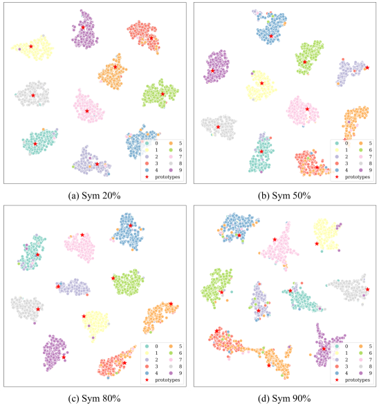
Figure 6: T-SNE visualizations of features and prototypes. The subplots show class distributions after training networks for 400 epochs on the CIFAR10 dataset with various noise ratios: (a) 20% symmetric, (b) 50% symmetric, (c) 80% symmetric, (d) 90% symmetric. Our proposed method effectively learns robust representations and class prototypes even with high noise ratios.

In Figure 7, we visualize the images that have the top-5 largest cosine similarity features to the prototypes of each class on the CIFAR10 dataset with 90% symmetric noise. Corresponding ground truth labels and given noisy labels are listed above each image. If the noisy label differs from the latent ground truth, it is colored in red; otherwise in green. We use a $\checkmark$ to indicate that an image has been correctly assigned to its corresponding cluster and $\boldsymbol{\times}$ if not. As can be seen, most images have been assigned to its ground truth cluster, which shows the effectiveness of our method.

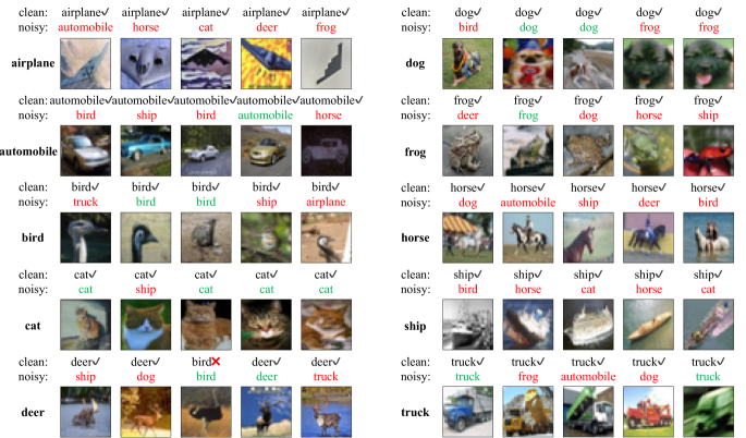
Figure 7: Visualization of images and labels in CIFAR10 dataset with 90% label noise. For each class, we select and show those images with top-5 largest cosine similarity features to the prototypes. Most of the image features are correctly assigned to the correct class, which demonstrates the effectiveness of our proposed PLR loss.

References

- Arazo et al. [2019] Eric Arazo, Diego Ortego, Paul Albert, Noel O’Connor, and Kevin McGuinness. Unsupervised label noise modeling and loss correction. In International Conference on Machine Learning, pages 312–321. PMLR, 2019.
- Arpit et al. [2017] Devansh Arpit, Stanisław Jastrzębski, Nicolas Ballas, David Krueger, Emmanuel Bengio, Maxinder S Kanwal, Tegan Maharaj, Asja Fischer, Aaron Courville, Yoshua Bengio, et al. A closer look at memorization in deep networks. In International Conference on Machine Learning, pages 233–242. PMLR, 2017.
- Bai et al. [2021] Yingbin Bai, Erkun Yang, Bo Han, Yanhua Yang, Jiatong Li, Yinian Mao, Gang Niu, and Tongliang Liu. Understanding and improving early stopping for learning with noisy labels. Advances in Neural Information Processing Systems, 34:24392–24403, 2021.
- Berthelot et al. [2019] David Berthelot, Nicholas Carlini, Ian Goodfellow, Nicolas Papernot, Avital Oliver, and Colin A Raffel. Mixmatch: A holistic approach to semi-supervised learning. Advances in Neural Information Processing Systems, 32, 2019.
- Caron et al. [2020] Mathilde Caron, Ishan Misra, Julien Mairal, Priya Goyal, Piotr Bojanowski, and Armand Joulin. Unsupervised learning of visual features by contrasting cluster assignments. Advances in Neural Information Processing Systems, 33:9912–9924, 2020.
- Cha and Cho [2012] Youngchul Cha and Junghoo Cho. Social-network analysis using topic models. In Proceedings of the 35th international ACM SIGIR conference on Research and development in information retrieval, pages 565–574, 2012.
- Chen et al. [2021] Junya Chen, Zhe Gan, Xuan Li, Qing Guo, Liqun Chen, Shuyang Gao, Tagyoung Chung, Yi Xu, Belinda Zeng, Wenlian Lu, et al. Simpler, faster, stronger: Breaking the log-k curse on contrastive learners with flatnce. arXiv preprint arXiv:2107.01152, 2021.
- Chen et al. [2020] Ting Chen, Simon Kornblith, Mohammad Norouzi, and Geoffrey Hinton. A simple framework for contrastive learning of visual representations. In International Conference on Machine Learning, pages 1597–1607. PMLR, 2020.
- Chen and Gupta [2015] Xinlei Chen and Abhinav Gupta. Webly supervised learning of convolutional networks. In Proceedings of the IEEE/CVF International Conference on Computer Vision, pages 1431–1439, 2015.
- Cubuk et al. [2019] Ekin D Cubuk, Barret Zoph, Dandelion Mane, Vijay Vasudevan, and Quoc V Le. Autoaugment: Learning augmentation strategies from data. In Proceedings of the IEEE/CVF Conference on Computer Vision and Pattern Recognition, pages 113–123, 2019.
- Deng et al. [2020] Pengfei Deng, Jingkai Ren, Shengbo Lv, Jiadong Feng, and Hongyuan Kang. Multi-label image recognition in anime illustration with graph convolutional networks. In Proceedings of the AAAI Conference on Artificial Intelligence, 2020.
- Ghosh and Lan [2021] Aritra Ghosh and Andrew Lan. Contrastive learning improves model robustness under label noise. In Proceedings of the IEEE/CVF Conference on Computer Vision and Pattern Recognition, pages 2703–2708, 2021.
- Han et al. [2018] Bo Han, Quanming Yao, Xingrui Yu, Gang Niu, Miao Xu, Weihua Hu, Ivor Tsang, and Masashi Sugiyama. Co-teaching: Robust training of deep neural networks with extremely noisy labels. Advances in Neural Information Processing Systems, 31, 2018.
- He et al. [2016a] Kaiming He, Xiangyu Zhang, Shaoqing Ren, and Jian Sun. Deep residual learning for image recognition. In Proceedings of the IEEE/CVF Conference on Computer Vision and Pattern Recognition, pages 770–778, 2016a.
- He et al. [2016b] Kaiming He, Xiangyu Zhang, Shaoqing Ren, and Jian Sun. Identity mappings in deep residual networks. In Proceedings of the European Conference on Computer Vision, pages 630–645. Springer, 2016b.
- He et al. [2020] Kaiming He, Haoqi Fan, Yuxin Wu, Saining Xie, and Ross Girshick. Momentum contrast for unsupervised visual representation learning. In Proceedings of the IEEE/CVF Conference on Computer Vision and Pattern Recognition, pages 9729–9738, 2020.
- Huang et al. [2020] Lang Huang, Chao Zhang, and Hongyang Zhang. Self-adaptive training: beyond empirical risk minimization. Advances in Neural Information Processing Systems, 33:19365–19376, 2020.
- Huang et al. [2023] Zhizhong Huang, Junping Zhang, and Hongming Shan. Twin contrastive learning with noisy labels. In Proceedings of the IEEE/CVF Conference on Computer Vision and Pattern Recognition, pages 11661–11670, 2023.
- Jiang et al. [2018] Lu Jiang, Zhengyuan Zhou, Thomas Leung, Li-Jia Li, and Li Fei-Fei. Mentornet: Learning data-driven curriculum for very deep neural networks on corrupted labels. In International Conference on Machine Learning, pages 2304–2313. PMLR, 2018.
- Karim et al. [2022] Nazmul Karim, Mamshad Nayeem Rizve, Nazanin Rahnavard, Ajmal Mian, and Mubarak Shah. Unicon: Combating label noise through uniform selection and contrastive learning. In Proceedings of the IEEE/CVF Conference on Computer Vision and Pattern Recognition, pages 9676–9686, 2022.
- Khosla et al. [2020] Prannay Khosla, Piotr Teterwak, Chen Wang, Aaron Sarna, Yonglong Tian, Phillip Isola, Aaron Maschinot, Ce Liu, and Dilip Krishnan. Supervised contrastive learning. Advances in Neural Information Processing Systems, 33:18661–18673, 2020.
- Kim et al. [2019] Youngdong Kim, Junho Yim, Juseung Yun, and Junmo Kim. Nlnl: Negative learning for noisy labels. In Proceedings of the IEEE/CVF International Conference on Computer Vision, pages 101–110, 2019.
- Krause et al. [2016] Jonathan Krause, Benjamin Sapp, Andrew Howard, Howard Zhou, Alexander Toshev, Tom Duerig, James Philbin, and Li Fei-Fei. The unreasonable effectiveness of noisy data for fine-grained recognition. In Proceedings of the European Conference on Computer Vision, pages 301–320. Springer, 2016.
- Krizhevsky et al. [2009] Alex Krizhevsky, Geoffrey Hinton, et al. Learning multiple layers of features from tiny images. 2009.
- Krizhevsky et al. [2017] Alex Krizhevsky, Ilya Sutskever, and Geoffrey E Hinton. Imagenet classification with deep convolutional neural networks. Communications of the ACM, 60(6):84–90, 2017.
- Kuznetsova et al. [2020] Alina Kuznetsova, Hassan Rom, Neil Alldrin, Jasper Uijlings, Ivan Krasin, Jordi Pont-Tuset, Shahab Kamali, Stefan Popov, Matteo Malloci, Alexander Kolesnikov, et al. The open images dataset v4: Unified image classification, object detection, and visual relationship detection at scale. International Journal of Computer Vision, 128(7):1956–1981, 2020.
- Le and Yang [2015] Ya Le and Xuan Yang. Tiny imagenet visual recognition challenge. CS 231N, 7(7):3, 2015.
- Li et al. [2019] Junnan Li, Richard Socher, and Steven CH Hoi. Dividemix: Learning with noisy labels as semi-supervised learning. In International Conference on Learning Representations, 2019.
- Li et al. [2020a] Junnan Li, Caiming Xiong, and Steven Hoi. Mopro: Webly supervised learning with momentum prototypes. In International Conference on Learning Representations, 2020a.
- Li et al. [2021] Junnan Li, Caiming Xiong, and Steven CH Hoi. Learning from noisy data with robust representation learning. In Proceedings of the IEEE/CVF International Conference on Computer Vision, pages 9485–9494, 2021.
- Li et al. [2020b] Mingchen Li, Mahdi Soltanolkotabi, and Samet Oymak. Gradient descent with early stopping is provably robust to label noise for overparameterized neural networks. In International conference on artificial intelligence and statistics, pages 4313–4324. PMLR, 2020b.
- Li et al. [2022] Shikun Li, Xiaobo Xia, Shiming Ge, and Tongliang Liu. Selective-supervised contrastive learning with noisy labels. In Proceedings of the IEEE/CVF Conference on Computer Vision and Pattern Recognition, pages 316–325, 2022.
- Li et al. [2017] Wen Li, Limin Wang, Wei Li, Eirikur Agustsson, and Luc Van Gool. Webvision database: Visual learning and understanding from web data. arXiv preprint arXiv:1708.02862, 2017.
- Liu et al. [2020] Sheng Liu, Jonathan Niles-Weed, Narges Razavian, and Carlos Fernandez-Granda. Early-learning regularization prevents memorization of noisy labels. Advances in Neural Information Processing Systems, 33:20331–20342, 2020.
- Liu et al. [2011] Wei Liu, Yu-Gang Jiang, Jiebo Luo, and Shih-Fu Chang. Noise resistant graph ranking for improved web image search. In Proceedings of the IEEE/CVF Conference on Computer Vision and Pattern Recognition, pages 849–856, 2011.
- Mahajan et al. [2018] Dhruv Mahajan, Ross Girshick, Vignesh Ramanathan, Kaiming He, Manohar Paluri, Yixuan Li, Ashwin Bharambe, and Laurens Van Der Maaten. Exploring the limits of weakly supervised pretraining. In Proceedings of the European Conference on Computer Vision, pages 181–196, 2018.
- Nishi et al. [2021] Kento Nishi, Yi Ding, Alex Rich, and Tobias Hollerer. Augmentation strategies for learning with noisy labels. In Proceedings of the IEEE/CVF Conference on Computer Vision and Pattern Recognition, pages 8022–8031, 2021.
- Oord et al. [2018] Aaron van den Oord, Yazhe Li, and Oriol Vinyals. Representation learning with contrastive predictive coding. arXiv preprint arXiv:1807.03748, 2018.
- Ortego et al. [2021] Diego Ortego, Eric Arazo, Paul Albert, Noel E O’Connor, and Kevin McGuinness. Multi-objective interpolation training for robustness to label noise. In Proceedings of the IEEE/CVF Conference on Computer Vision and Pattern Recognition, pages 6606–6615, 2021.
- Reed et al. [2014] Scott Reed, Honglak Lee, Dragomir Anguelov, Christian Szegedy, Dumitru Erhan, and Andrew Rabinovich. Training deep neural networks on noisy labels with bootstrapping. arXiv preprint arXiv:1412.6596, 2014.
- Ren et al. [2015] Shaoqing Ren, Kaiming He, Ross Girshick, and Jian Sun. Faster r-cnn: Towards real-time object detection with region proposal networks. Advances in Neural Information Processing Systems, 28, 2015.
- Ronneberger et al. [2015] Olaf Ronneberger, Philipp Fischer, and Thomas Brox. U-net: Convolutional networks for biomedical image segmentation. In Medical Image Computing and Computer-Assisted Intervention–MICCAI 2015: 18th International Conference, Munich, Germany, October 5-9, 2015, Proceedings, Part III 18, pages 234–241. Springer, 2015.
- Russakovsky et al. [2015] Olga Russakovsky, Jia Deng, Hao Su, Jonathan Krause, Sanjeev Satheesh, Sean Ma, Zhiheng Huang, Andrej Karpathy, Aditya Khosla, Michael Bernstein, Alexander C. Berg, and Li Fei-Fei. ImageNet Large Scale Visual Recognition Challenge. International Journal of Computer Vision, 115(3):211–252, 2015.
- Sachdeva et al. [2023] Ragav Sachdeva, Filipe Rolim Cordeiro, Vasileios Belagiannis, Ian Reid, and Gustavo Carneiro. Scanmix: Learning from severe label noise via semantic clustering and semi-supervised learning. Pattern Recognition, 134:109121, 2023.
- Sohn et al. [2020] Kihyuk Sohn, David Berthelot, Nicholas Carlini, Zizhao Zhang, Han Zhang, Colin A Raffel, Ekin Dogus Cubuk, Alexey Kurakin, and Chun-Liang Li. Fixmatch: Simplifying semi-supervised learning with consistency and confidence. Advances in Neural Information Processing Systems, 33:596–608, 2020.
- Song et al. [2019] Hwanjun Song, Minseok Kim, Dongmin Park, and Jae-Gil Lee. How does early stopping help generalization against label noise? arXiv preprint arXiv:1911.08059, 2019.
- Sukhbaatar et al. [2015] Sainbayar Sukhbaatar, Joan Bruna, Manohar Paluri, Lubomir Bourdev, and Rob Fergus. Training convolutional networks with noisy labels. In International Conference on Learning Representations, 2015.
- Szegedy et al. [2017] Christian Szegedy, Sergey Ioffe, Vincent Vanhoucke, and Alexander Alemi. Inception-v4, inception-resnet and the impact of residual connections on learning. In Proceedings of the AAAI Conference on Artificial Intelligence, 2017.
- Tanaka et al. [2018] Daiki Tanaka, Daiki Ikami, Toshihiko Yamasaki, and Kiyoharu Aizawa. Joint optimization framework for learning with noisy labels. In Proceedings of the IEEE/CVF Conference on Computer Vision and Pattern Recognition, pages 5552–5560, 2018.
- Van der Maaten and Hinton [2008] Laurens Van der Maaten and Geoffrey Hinton. Visualizing data using t-sne. Journal of machine learning research, 9(11), 2008.
- Wang et al. [2022] Haobo Wang, Ruixuan Xiao, Yiwen Dong, Lei Feng, and Junbo Zhao. Promix: Combating label noise via maximizing clean sample utility. arXiv preprint arXiv:2207.10276, 2022.
- Wei et al. [2020] Hongxin Wei, Lei Feng, Xiangyu Chen, and Bo An. Combating noisy labels by agreement: A joint training method with co-regularization. In Proceedings of the IEEE/CVF Conference on Computer Vision and Pattern Recognition, pages 13726–13735, 2020.
- Wu et al. [2018] Zhirong Wu, Yuanjun Xiong, Stella X Yu, and Dahua Lin. Unsupervised feature learning via non-parametric instance discrimination. In Proceedings of the IEEE/CVF Conference on Computer Vision and Pattern Recognition, pages 3733–3742, 2018.
- Xiao et al. [2015] Tong Xiao, Tian Xia, Yi Yang, Chang Huang, and Xiaogang Wang. Learning from massive noisy labeled data for image classification. In Proceedings of the IEEE/CVF Conference on Computer Vision and Pattern Recognition, pages 2691–2699, 2015.
- Yan et al. [2022] Jiexi Yan, Lei Luo, Chenghao Xu, Cheng Deng, and Heng Huang. Noise is also useful: Negative correlation-steered latent contrastive learning. In Proceedings of the IEEE/CVF Conference on Computer Vision and Pattern Recognition, pages 31–40, 2022.
- Yi and Wu [2019] Kun Yi and Jianxin Wu. Probabilistic end-to-end noise correction for learning with noisy labels. In Proceedings of the IEEE/CVF Conference on Computer Vision and Pattern Recognition, pages 7017–7025, 2019.
- Yu et al. [2020] Tianhe Yu, Saurabh Kumar, Abhishek Gupta, Sergey Levine, Karol Hausman, and Chelsea Finn. Gradient surgery for multi-task learning. Advances in Neural Information Processing Systems, 33:5824–5836, 2020.
- Yu et al. [2019] Xingrui Yu, Bo Han, Jiangchao Yao, Gang Niu, Ivor Tsang, and Masashi Sugiyama. How does disagreement help generalization against label corruption? In International Conference on Machine Learning, pages 7164–7173. PMLR, 2019.
- Zhang et al. [2021] Chiyuan Zhang, Samy Bengio, Moritz Hardt, Benjamin Recht, and Oriol Vinyals. Understanding deep learning (still) requires rethinking generalization. Communications of the ACM, 64(3):107–115, 2021.
- Zhang and Yao [2020] Hui Zhang and Quanming Yao. Decoupling representation and classifier for noisy label learning. arXiv preprint arXiv:2011.08145, 2020.
- Zhang et al. [2018] Hongyi Zhang, Moustapha Cisse, Yann N Dauphin, and David Lopez-Paz. mixup: Beyond empirical risk minimization. In International Conference on Learning Representations, 2018.
- Zheltonozhskii et al. [2022] Evgenii Zheltonozhskii, Chaim Baskin, Avi Mendelson, Alex M Bronstein, and Or Litany. Contrast to divide: Self-supervised pre-training for learning with noisy labels. In Proceedings of the IEEE/CVF Winter Conference on Applications of Computer Vision, pages 1657–1667, 2022.