Triangle singularity in the $J/\psi\to\phi\pi^{+}a_{0}^{-}(\pi^{-}\eta),\;\phi\pi^{-}a_{0}^{+}(\pi^{+}\eta)$ decays

Abstract

We study the $J/\psi\to\phi\pi^{+}a_{0}(980)^{-}(a_{0}^{-}\to\pi^{-}\eta)$ decay, evaluating the double mass distribution in terms of the $\pi^{-}\eta$ and $\pi^{+}a_{0}$ invariant masses. We show that the $\pi^{-}\eta$ mass distribution exhibits the typical cusp structure of the $a_{0}(980)$ seen in recent high statistics experiments, and the $\pi^{+}a_{0}$ spectrum shows clearly a peak around $M_{\rm inv}(\pi^{+}a_{0})=1420\,{\rm MeV}$, corresponding to a triangle singularity. When integrating over the two invariant masses we find a branching ratio for this decay of the order of $10^{-5}$, which is easily accessible in present laboratories.

I Introduction

Triangle singularities (TS), introduced in Refs. karplus ; landau , correspond to processes in which there is a triangle diagram in the amplitude, where the three intermediate particles can be placed simultaneously on shell, representing a reaction that can occur at the classical level norton , in which case the amplitude becomes infinite in the limit of zero width of the intermediate particles. The issue has experienced a revival in recent years, one of the reasons, among many, being the fact that after early claims by the COMPASS Collaboration of the “$a_{1}(1420)$” discovery adolf , it was soon explained as a consequence of a triangle singularity in which the $a_{1}(1260)$ resonance decays into $K^{*}\bar{K},\,K^{*}\to\pi K$, and then $K\bar{K}$ fuse to give the $f_{0}(980)$ resonance, the $\pi f_{0}(980)$ being the observed decay mode qzhao ; misha ; acetidai ; Alexeev . Earlier than that, there was an interpretation of the isospin violating decay $\eta(1405)\to f_{0}(980)\pi^{0}$ beseta also in terms of a triangle singularity wuzou ; fcaliang ; wuwu , and more recently the interpretation of the $pp\to\pi^{+}d$ reaction serre ; said in terms of a triangle singularity ikenomolina . More examples were given in the interpretation of the $J/\psi\to\eta\pi^{0}\phi$ reaction in Ref. jingsakaiguo , and in the enhanced isospin violation in $D_{s}^{+}\to\pi^{+}\pi^{0}a_{0}(980)[f_{0}(980)]$ or $\bar{B}_{s}^{0}\to J/\psi\pi^{0}a_{0}(980)[f_{0}(980)]$ sakailiang ; sakailiaxie . A long list of reactions showing effects of triangle singularities can be seen in Table 1 of the review paper reviewts . Also, a reformulation of the TS has been provided in Ref. bayaracetiguo , which is at the same time pedagogical and practical.

The issue has emerged once more due to the recent BESIII paper besrecent , improving considerably on earlier measurements of the $J/\psi\to\eta\pi^{0}\phi$ reaction, where the ideas of Ref. jingsakaiguo could be tested. Indeed, that reaction develops a TS in the $\pi^{0}\phi$ mass distribution, peaking around $M(\phi\pi^{0})\sim 1400$ MeV, where a clear signal is seen in Ref. besrecent . Yet, the interpretation of the peak is delicate, because, as discussed in Ref. jingsakaiguo , the peak is masked by a tree level contribution which has also a singular behaviour. Indeed, the TS mechanism proceeds via the diagrams of Figs. 1 (a) and (b), but the same final state is reached by the tree level diagrams of Figs. 1 (c) and (d).

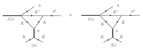
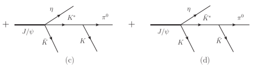
Figure 1: Mechanisms in $J/\psi\to\eta\pi^{0}\phi\;(\phi\to K\bar{K})$: (a), (b) TS; (c), (d) the tree level.

Then, Schmid theorem schmid comes into play because if the triangle diagrams develop a TS they can be reabsorbed into the tree level diagrams with a simple change of phase, and the decay width is not affected by the TS diagrams. A thorough review of this issue was done in Ref. vinischmid , showing that the theorem holds in the limit of the $K^{*}$ width (in the present case) going to zero, and when there are no inelastic channels. The message of Ref. vinischmid is that all diagrams must be calculated, and that normally the tree level diagrams are mostly responsible for the mass distributions, with the effects of the TS diagrams being diluted in these distributions.

In view of these problems we look now at a related reaction where a TS develops, which is not masked by the effects of tree level and Schmid theorem. The reaction is $J/\psi\to\phi\pi^{-}a_{0}(980)^{+}(\pi^{+}\eta),\;\phi\pi^{+}a_{0}(980)^{-}(\pi^{-}\eta)$. The mechanism is similar to that in Figs. 1(a) and 1(b), with $\eta$ replaced by $\phi$, but the intermediate $K\bar{K}$ produce the $a_{0}(980)$ resonance which decays to $\pi\eta$. Then, the tree level diagrams with $K\bar{K}$ production do not interfere with the triangle diagram, which also develops a singularity in the $\pi a_{0}(980)$ mass distribution. It is easy to see where we should expect the singularity applying Eq. (18) of Ref. bayaracetiguo (with $m_{a_{0}}$ slightly larger than $2\,m_{K}$), and one finds that a singularity should appear at $M_{\rm inv}(\pi a_{0})\sim 1417$ MeV. The purpose of the present work is to do a detailed study of the reaction and make a realistic prediction of the shape and size of the $\pi a_{0}(980)$ mass distribution in that reaction.

II Formalism

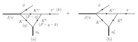
Figure 2: Triangle diagrams for $J/\psi\to\phi\pi^{+}a_{0}^{-}$ decay (a) and $J/\psi\to\phi\pi^{-}a_{0}^{+}$ decay (b). Figs. (c) and (d) illustrate the processes of (a) and (b) respectively, with a clear depiction of the decay channel of $a_{0}^{-}$ and $a_{0}^{+}$. In Fig. (a), the momenta of the particles are shown, where $P=p_{J/\psi}-p_{\phi}$.

We look at the diagrams of Fig. 2. The diagrams of Figs. 2(a) and 2(b) show the coalescence processes where the $a_{0}^{-},\,a_{0}^{+}$ are produced, independent on the decay channel in which the $a_{0}$ resonances are observed. The diagrams of Figs. 2(c) and 2(d) show the explicit reaction, with four body final state when the $a_{0}^{-/+}$ decay into $\pi^{-/+}\eta$, the only sizeable decay channel. We shall consider this final state, but it is practical to consider first the coalescence processes, with only three particles in the final state. We consider the reactions $J/\psi\to\phi\pi^{-}a_{0}^{+}$ and $J/\psi\to\phi\pi^{+}a_{0}^{-}$ as different reactions and will concentrate on the first one. The same distributions would be obtained for the second reaction.

In order to be able to determine absolute rates for the $J/\psi\to\phi\pi^{-}a_{0}^{+}\;(J/\psi\to\phi\pi a_{0})$ reaction we need information on the $J/\psi\to\phi K^{*-}K^{+}$ reaction, which we take from experiment. On the other hand, the dynamics of $K^{*}\to K\pi$ and $K\bar{K}\to a_{0}\to\pi\eta$ are well known, and for the $K\bar{K}\to a_{0}\to\pi\eta$ amplitudes we shall use the chiral unitary approach npa ; kaiser ; markushin ; juan .

II.1 The $J/\psi\to\phi K^{*}\bar{K}$ reaction

In the Particle Data Group (PDG) pdg , we have the branching ratio,

$$\text{Br}(J/\psi\to\phi K^{*}(892)\bar{K}+c.c.)=(2.18\pm 0.23)\times 10^{-3}.$$ (1)

However, we are only interested in $J/\psi\to\phi K^{*-}K^{+}$. It is easy to see the rate for this particular channel using isospin and $C$ parity arguments. With the isospin convention for the multiplets $(K^{+},\,K^{0})$, $(\bar{K}^{0},\,-K^{-})$, $(K^{*+},\,K^{*0})$, $(\bar{K}^{*0},\,-K^{*-})$, the $K^{*}\bar{K}$ isospin zero states demanded in the reaction of Eq. (1) are given by

$$|K^{*}\bar{K},\;I=0\rangle=-\frac{1}{\sqrt{2}}\;\left(K^{*+}K^{-}+K^{*0}\bar{K}^{0}\right),$$ (2)

$$|\bar{K}^{*}K,\;I=0\rangle=\frac{1}{\sqrt{2}}\;\left(\bar{K}^{*0}K^{0}+K^{*-}K^{+}\right).$$

Knowing that $CK^{*+}=-K^{*-}$, $CK^{+}=K^{-}$ etc, the right combination for $J/\psi\to\phi K^{*}\bar{K}+c.c.$ is given by

$$J/\psi\to\phi\left(K^{*+}K^{-}+K^{*0}\bar{K}^{0}-K^{*-}K^{+}-\bar{K}^{*0}K^{0}\right),$$ (3)

which means that the branching ratio of $J/\psi\to\phi K^{*+}K^{-}$ will be one fourth of the one in Eq. (1),

$$\text{Br}(J/\psi\to\phi K^{*+}K^{-})=(0.55\pm 0.06)\times 10^{-3}.$$ (4)

Furthermore, the structure of the amplitude in $S$-wave is given by

$$V_{J/\psi,\;\phi K^{*+}K^{-}}=C\;\vec{\epsilon}_{J/\psi}\cdot\left(\vec{\epsilon}_{\phi}\times\vec{\epsilon}_{K^{*}}\right).$$ (5)

We can determine $C$ from the rate of Eq. (4) using

$$\dfrac{d\Gamma_{J/\psi\to\phi K^{*+}K^{-}}}{dM_{\rm inv}(K^{*+}K^{-})}=\dfrac{1}{(2\pi)^{3}}\;\dfrac{1}{4M_{J/\psi}^{2}}\;p_{\phi}\,\tilde{p}_{K^{-}}\,\overline{\sum}\sum|t|^{2},$$ (6)

with

$$p_{\phi}=\dfrac{\lambda^{1/2}(M_{J/\psi}^{2},\,M_{\phi}^{2},\,M_{\rm inv}^{2}(K^{*+}K^{-}))}{2M_{J/\psi}},$$ (7)

$$\tilde{p}_{K^{-}}=\dfrac{\lambda^{1/2}(M_{\rm inv}^{2}(K^{*+}K^{-}),\,M_{K^{*+}}^{2},\,M_{K^{-}}^{2})}{2M_{\rm inv}(K^{*+}K^{-})},$$

and $\overline{\sum}\sum|t|^{2}$ stands for the average and sum over the polarizations of $J/\psi$, $\phi$, and $K^{*}$ mesons, with $t$ defined in Eq. (5). Therefore,

$$\overline{\sum}\sum|t|^{2}=2\,C^{2}.$$ (8)

Then we find

$$\dfrac{C^{2}}{\Gamma_{J/\psi}}=\dfrac{\text{Br}(J/\psi\to\phi K^{*+}K^{-})}{\displaystyle\int\dfrac{2}{(2\pi)^{3}}\;\dfrac{1}{4M_{J/\psi}^{2}}\,p_{\phi}\,\tilde{p}_{K^{-}}\;dM_{\rm inv}(K^{*+}K^{-})},$$ (9)

from where we obtain

$$\dfrac{C^{2}}{\Gamma_{J/\psi}}=1.381\times 10^{-2}\quad(\text{MeV}^{-1}),$$ (10)

which we will use to evaluate the strength of the triangle mechanism.

II.2 The $a_{0}^{-}\to K^{-}K^{0}$ coupling and $K^{*}\to K\pi$ vertex

The $K^{*+}\to K^{0}\pi^{+}$ coupling is easily obtained from the standard Lagrangian

$${\cal L}=-ig\langle[P,\;\partial_{\mu}P]V^{\mu}\rangle,$$ (11)

with $P$ and $V$ representing the SU(3) $q\bar{q}$ matrix written in terms of pseudoscalar or vector mesons, respectively Ikeno:2019grj . The coupling $g$ is defined as $g=\frac{M_{V}}{2f}$, where $M_{V}=800$ MeV and $f=93$ MeV. This yields the vertex

$$-it=-ig\epsilon_{j}(K^{*})(2k+q)^{j},$$ (12)

which is evaluated in the frame where we take $\vec{P}=\vec{p}_{J/\psi}-\vec{p}_{\phi}=0$. In this frame, we can neglect the $\epsilon^{0}$ component of the $K^{*}$ sakairamos .

The coupling of $a_{0}\to K^{+}K^{-}$ needed in the evaluation of the diagram of Fig. 2(a) without further decay of $a_{0}\to\pi^{-}\eta$ can be accounted for in the following way. It is clear that if we evaluate the $J/\psi\to\phi\pi^{+}\pi^{-}\eta$ decay we would only need the $K^{-}K^{0}\to\pi^{-}\eta$ amplitude. The coalescence decay $J/\psi\to\phi\pi^{+}a_{0}^{-}$ should also be able to be calculated using the $K\bar{K}$ amplitudes and this is formally done as discussed below.

Assuming that, close to the peak of the $a_{0}(980)$,

$$t_{K^{-}K^{0},\,K^{-}K^{0}}(M_{\rm inv})=\frac{g^{2}_{a_{0},\,K^{-}K^{0}}}{M^{2}_{\rm inv}-m^{2}_{a_{0}}+iM_{\rm inv}\Gamma_{a_{0}}},$$ (13)

then, using Cauchy’s integration we find immediately

$$g^{2}_{a_{0},\,K^{-}K^{0}}=-\frac{1}{\pi}\int dM^{2}_{\rm inv}\;\text{Im}\,t_{K^{-}K^{0},\,K^{-}K^{0}}(M_{\rm inv}),$$ (14)

which is also trivially obtained in the limit of $\Gamma_{a_{0}}\to 0$ using

$$\text{Im}\,\left[\left(M^{2}_{\rm inv}-m^{2}_{a_{0}}\right)+i\epsilon\right]^{-1}=-i\pi\delta\left(M^{2}_{\rm inv}-m^{2}_{a_{0}}\right).$$ (15)

In the coalescence process we will use Eq. (14) in the evaluation of the $|t_{\rm TS}|^{2}$ of the triangle diagram. We will have

$$\dfrac{d\Gamma_{J/\psi,\to\phi\pi^{+}a_{0}^{-}}}{dM_{\rm inv}(\pi^{+}a_{0}^{-})}=\dfrac{1}{(2\pi)^{3}}\;\dfrac{1}{4M_{J/\psi}^{2}}\;p_{\phi}\;\tilde{p}_{\pi^{+}}\;\overline{\sum}|t_{\rm TS}|^{2},$$ (16)

where

$$p_{\phi}=\dfrac{\lambda^{1/2}(M_{J/\psi}^{2},\,m_{\phi}^{2},\,M_{\rm inv}^{2}(\pi^{+}a_{0}^{-}))}{2M_{J/\psi}},$$ (17)

$$\tilde{p}_{\pi^{+}}=\dfrac{\lambda^{1/2}(M_{\rm inv}^{2}(\pi^{+}a_{0}^{-}),\,m_{\pi^{+}}^{2},\,m_{a_{0}^{-}}^{2})}{2M_{\rm inv}(\pi^{+}a_{0}^{-})},$$ (18)

with $t_{\rm TS}$ corresponding to the amplitude for the process of Fig. 2(a). Since $|t_{\rm TS}|^{2}$ contains $g^{2}_{a_{0},\,K^{-}K^{0}}$, given in Eq. (14), we can undo the $dM^{2}_{\rm inv}$ integration in Eq. (16) and write

$$\dfrac{d^{2}\Gamma_{J/\psi,\to\phi\pi^{+}a_{0}^{-}(\pi^{-}\eta)}}{dM_{\rm inv}(\pi^{-}\eta)\;dM_{\rm inv}(\pi^{+}a_{0}^{-})}= -\dfrac{1}{\pi}\;2M_{\rm inv}(\pi^{-}\eta)\;\text{Im}\,t_{K^{-}K^{0},\,K^{-}K^{0}}(M_{\rm inv}(\pi^{-}\eta))$$ (19)

$$\times\dfrac{1}{(2\pi)^{3}}\;\dfrac{1}{4M_{J/\psi}^{2}}\;p_{\phi}\;\tilde{p}_{\pi^{+}}^{\prime}\overline{\sum}|\tilde{t}_{\rm TS}|^{2},$$

where $\tilde{p}_{\pi^{+}}^{\prime}$ is given by Eq. (18) substituting $m_{a_{0}^{-}}$ by $M_{\rm inv}(\pi^{-}\eta)$, and $|\tilde{t}_{\rm TS}|^{2}$ is the magnitude $|t_{\rm TS}|^{2}$ where we remove $g^{2}_{a_{0},\,K^{-}K^{0}}$.

Eq. (19) can be immediately reinterpreted. Indeed, in the evaluation of $|t_{\rm TS}|^{2}$ for the triangle diagram of Fig. 2(c), we will need $|t_{K^{-}K^{0},\;\pi^{-}\eta}|^{2}$ along with the extra phase space for $\pi^{-}\eta$ with respect to Fig. 2(a). But $|t_{K^{-}K^{0},\;\pi^{-}\eta}|^{2}$ times the phase space for $a_{0}^{-}\to\pi^{-}\eta$ decay is what is given by $\text{Im}\,t_{K^{-}K^{0},\;K^{-}K^{0}}$ via the optical theorem. The derivation done, however, has served to go from the differential mass distribution in the three body final state to the one of the four body in a simple and intuitive way.

II.3 The triangle amplitude

In Fig. 2(a), we show the momenta of the particles. Since we are concerned about the triangle singularity, occurring when the intermediate particles are all on shell, we can simplify the calculation (see Ref. bayaracetiguo ) taking the positive energy part of the propagators, which is the one that can go on shell. Hence for a $K^{-}$ propagator we would write

$$\dfrac{1}{q^{2}-m_{K}^{2}+i\epsilon}=\dfrac{1}{2\omega(\vec{q}\,)}\;\left(\dfrac{1}{q^{0}-\omega_{K}(\vec{q}\,)+i\epsilon}-\dfrac{1}{q^{0}+\omega_{K}(\vec{q}\,)-i\epsilon}\right),$$ (20)

with $\omega_{K}(\vec{q}\,)=\sqrt{\vec{q}\;^{2}+m_{K}^{2}}$, and with $q^{0}$ positive only the first term of the former equation can go on shell, and we shall then keep this term alone. This simplifies the expression for the loop amplitude which reads, removing the $g_{a_{0},\,K^{-}K^{0}}$ vertex:

$$-i\tilde{t}_{\rm TS}= -i\,C\int\dfrac{d^{4}q}{(2\pi)^{4}}\;\epsilon_{ijl}\;\epsilon_{i}(J/\psi)\;\epsilon_{j}(\phi)\;\epsilon_{l}(K^{*})\;(-i)g\;\epsilon_{m}(K^{*})\;(2k+q)_{m}$$ (21)

$$\times(-i)\;\dfrac{1}{2\omega_{K^{-}}(\vec{q}\,)}\;\dfrac{1}{2\omega_{K^{0}}(\vec{q}+\vec{k})}\;\dfrac{1}{2\omega_{K^{*+}}(\vec{q}\,)}\;\dfrac{i}{q^{0}-\omega_{K^{-}}(\vec{q}\,)+i\epsilon}$$

$$\times\frac{i}{P^{0}-q^{0}-\omega_{K^{*+}}(\vec{q}\,)+i\frac{\Gamma_{K^{*}}}{2}}\;\dfrac{i}{P^{0}-q^{0}-k^{0}-\omega_{K^{0}}(\vec{q}+\vec{k}\,)+i\epsilon},$$

with $\omega_{K^{-}}(\vec{q}\,)=\sqrt{\vec{q}\;^{2}+m_{K}^{2}}$, $\omega_{K^{*+}}(\vec{q}\,)=\sqrt{\vec{q}\;^{2}+m_{K^{*}}^{2}}$, where we have explicitly taken into account the $K^{*}$ width in the $K^{*}$ propagator, and $P^{0}$, $k^{0}$ are given by

$$P^{0}=M_{\rm inv}(\pi^{+}a_{0}^{-}),$$ (22)

$$k^{0}=\dfrac{P^{02}+m^{2}_{\pi^{+}}-M^{2}_{\rm inv}(\pi^{-}\eta)}{2P^{0}}.$$

We sum over the $K^{*}$ polarizations $\sum\epsilon_{l}(K^{*})\epsilon_{m}(K^{*})=\delta_{lm}$, and integrating analytically over $q^{0}$ in Eq. (21) using Cauchy’s residues, we obtain

$$\tilde{t}_{\rm TS}= g\,C\,\epsilon_{ijl}\;\epsilon_{i}(J/\psi)\;\epsilon_{j}(\phi)\;\int\dfrac{d^{3}q}{(2\pi)^{3}}\;(2k+q)_{l}\;\dfrac{1}{2\omega_{K^{-}}(\vec{q}\,)}\;\dfrac{1}{2\omega_{K^{*+}}(\vec{q}\,)}\;\dfrac{1}{2\omega_{K^{0}}(\vec{q}+\vec{k}\,)}$$ (23)

$$\times\dfrac{i}{P^{0}-\omega_{K^{-}}(\vec{q}\,)-\omega_{K^{*+}}(\vec{q}\,)+i\frac{\Gamma_{K^{*}}}{2}}\;\dfrac{i}{P^{0}-k^{0}-\omega_{K^{-}}(\vec{q}\,)-\omega_{K^{0}}(\vec{q}+\vec{k}\,)+i\epsilon}.$$

Next, considering that

$$\int d^{3}q\,F(\vec{q},\vec{k})\,q_{l}=k_{l}\,\int d^{3}q\;F(\vec{q},\vec{k})\;\dfrac{\vec{q}\cdot\vec{k}}{\vec{k}^{\,2}},$$ (24)

we finally write $\tilde{t}_{\rm TS}$ as

$$\tilde{t}_{\rm TS}=g\,C\,\epsilon_{ijl}\;\epsilon_{i}(J/\psi)\;\epsilon_{j}(\phi)\;k_{l}\;\tilde{t}^{\prime}_{\rm TS},$$ (25)

with

$$\tilde{t}^{\prime}_{\rm TS}= \int\dfrac{d^{3}q}{(2\pi)^{3}}\;\theta(q_{max}-|\vec{q}\;^{*}|\,)\;\left(2+\dfrac{\vec{q}\cdot\vec{k}}{\vec{k}^{\,2}}\right)\;\dfrac{1}{2\omega_{K^{-}}(\vec{q}\,)}\,\dfrac{1}{2\omega_{K^{*+}}(\vec{q}\,)}\,\dfrac{1}{2\omega_{K^{0}}(\vec{q}+\vec{k}\,)}$$ (26)

$$\times\dfrac{i}{P^{0}-\omega_{K^{-}}(\vec{q}\,)-\omega_{K^{*+}}(\vec{q}\,)+i\dfrac{\Gamma_{K^{*}}}{2}}\;\dfrac{i}{P^{0}-k^{0}-\omega_{K^{-}}(\vec{q}\,)-\omega_{K^{0}}(\vec{q}+\vec{k}\,)+i\epsilon},$$

and

$$\overline{\sum}\left|\tilde{t}_{\rm TS}\right|^{2}=\frac{2}{3}\,\vec{k}^{\,2}\,g^{2}\,C^{2}\;\left|\tilde{t}^{\prime}_{\rm TS}\right|^{2}.$$ (27)

In Eq. (26) we have introduced the factor $\theta(q_{max}-|\vec{q}\;^{*}|)$, where $\vec{q}\;^{*}$ is the $K^{-}$ momentum in the $\pi^{-}\eta$ rest frame given by bayaracetiguo

$$\vec{q}\;^{*}=\left[\left(\frac{E_{a_{0}}}{M_{\rm inv}(\pi^{-}\eta)}-1\right)\frac{\vec{q}\cdot\vec{k}}{\vec{k}^{\,2}}+\frac{q^{0}}{M_{\rm inv}(\pi^{-}\eta)}\right]\vec{k}+\vec{q}\;,$$ (28)

where $E_{a_{0}}=\sqrt{M^{2}_{\rm inv}+\vec{k}^{\,2}}$, $q^{0}=\sqrt{m^{2}_{K}+\vec{q}^{\;2}}$. This factor is demanded because in the cutoff regularization to obtain the $K\bar{K}$ scattering we have $t(\vec{q},\vec{q}^{\;\prime})=t\,\theta(q_{max}-|\vec{q}\,|)\,\theta(q_{max}-|\vec{q}\;^{\prime}|)$, with $q_{max}$ the cutoff momentum used in the regularization of the $G_{K\bar{K}}$ function danijuan .

II.4 $K\bar{K}$ amplitudes

We need to calculate the $t_{K^{-}K^{0},\;K^{-}K^{0}}$ amplitude, for which we use the chiral unitary approach. In this case, the $t_{K^{-}K^{0},K^{-}K^{0}}$ amplitude is one of the $T$-matrix elements, that is extracted by solving the Bethe-Salpeter equation in coupled-channels,

$$T=[1-VG]^{-1}V,$$ (29)

with $V$ the kernel encoding the $V_{ij}$ amplitudes from $i$- to $j$-channel. The channels considered are: $K\bar{K}$, $\pi\eta$, $\pi\pi$, and $\eta\eta$. The relevant $V_{ij}$ amplitudes among all the channels in our case are taken from Ref. lianglin , using explicitly the $\eta-\eta^{\prime}$ mixing of Ref. bramon (Eq. (A.4) of Ref. lianglin ). Furthermore, $G$ is a diagonal matrix with its elements $G_{l}$ corresponding to the loop function for the $l$-th channel. We take the $G_{l}$ loop function regularized by means of a cut-off $q_{\rm max}$ in the three-monentum,

$$G_{l}=\int_{|\vec{q}\,|<q_{\rm max}}\dfrac{d^{3}q}{(2\pi)^{3}}\;\dfrac{\omega_{1}+\omega_{2}}{2\omega_{1}\,\omega_{2}}\;\dfrac{1}{s-(\omega_{1}+\omega_{2})^{2}+i\epsilon}.$$ (30)

Since, only the zero charged components are considered in Ref. lianglin , we make use of the fact that $K^{-}K^{0}$ is the $I=1,\,I_{3}=-1$ component of $K\bar{K}$ and write,

$$t_{K^{-}K^{0},\;K^{-}K^{0}}=\frac{1}{2}\left(t_{K^{0}\bar{K}^{0},\;K^{0}\bar{K}^{0}}+t_{K^{+}K^{-},\;K^{+}K^{-}}-2\,t_{K^{0}\bar{K}^{0},\;K^{+}K^{-}}\right).$$ (31)

III Results

In Fig. 3, we show the factor $A\equiv[-\dfrac{2}{\pi}\;M_{\rm inv}(\pi^{-}\eta)\;{\rm Im}\,t_{K^{-}K^{0},K^{-}K^{0}}(M_{\rm inv}(\pi^{-}\eta))]$, which is involved in the double differential decay width of Eq. (19).

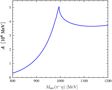
Figure 3: Factor $A\equiv\big{[}-\dfrac{2}{\pi}\;M_{\rm inv}(\pi^{-}\eta)\;{\rm Im}\,t_{K^{-}K^{0},K^{-}K^{0}}(M_{\rm inv}(\pi^{-}\eta))\big{]}$ as a function of $M_{\rm inv}(\pi^{-}\eta)$.

We can see a cusp-like structure around $M_{\rm inv}(\pi^{-}\eta)=m_{a_{0}}=980\,\textrm{ MeV}$, reflecting the spectral function of the $a_{0}(980)$.

Next, we discuss the amplitude $\tilde{t}^{\prime}_{\rm TS}$ of Eq. (26) and $\frac{1}{\Gamma_{J/\psi}}\,\frac{{\rm d}^{2}\Gamma_{J/\psi\to\phi\pi^{+}a_{0}(980)}}{{\rm d}M_{\rm inv}(\pi^{-}\eta)\;{\rm d}M_{\rm inv}(\pi^{+}a_{0})}$ of Eq. (19), which are functions of both $M_{\rm inv}(\pi^{-}\eta)$ and $M_{\rm inv}(\pi^{+}a_{0})$. We will present the results in three cases: 1) fixing $M_{\rm inv}(\pi^{-}\eta)=m_{a_{0}}=980\textrm{ MeV}$; 2) fixing $M_{\rm inv}(\pi^{+}a_{0})=1416\,\textrm{ MeV}$, where the TS occurs in the triangle loops of Fig. 2; and 3) integrating $\frac{1}{\Gamma_{J/\psi}}\,\frac{{\rm d}^{2}\Gamma_{J/\psi\to\phi\pi^{+}a_{0}(980)}}{{\rm d}M_{\rm inv}(\pi^{-}\eta)\;{\rm d}M_{\rm inv}(\pi^{+}a_{0})}$ over $M_{\rm inv}(\pi^{-}\eta)$.

III.1 Fixing $M_{\rm inv}(\pi^{-}\eta)=m_{a_{0}}=980\textrm{ MeV}$

In Fig. 4, we show results for ${\rm Re}\,\tilde{t}^{\prime}_{\rm TS}$, ${\rm Im}\,\tilde{t}^{\prime}_{\rm TS}$ and $|\tilde{t}^{\prime}_{\rm TS}|$ as a function of $M_{\rm inv}(\pi^{+}a_{0})$ while keeping $M_{\rm inv}(\pi^{-}\eta)$ fixed.

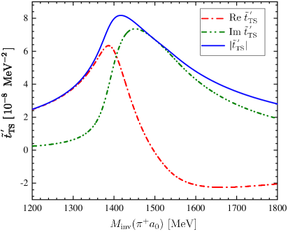
Figure 4: $\tilde{t}^{\prime}_{\rm TS}$ given by Eq. (26) as a function of $M_{\rm inv}(\pi^{+}a_{0})$ when fixing $M_{\rm inv}(\pi^{-}\eta)=m_{a_{0}}$.

The structure of the amplitude exhibits features typical of triangle singularities observed in other cases (see Fig. 5 of Ref. sakairamos , Fig. 4 of Ref. PavaoSakai , Fig. 3 of Ref. sakailiang , Fig. 4 of Ref. OsetRoca , Fig. 5 of Ref. DaiYu , Fig. 4 of Ref. LiangChen , Fig. 19 of Ref. GuoRev ). It has the imaginary part peaking around the $M_{\rm inv}(\pi^{+}a_{0})$, as provided by Eq. (18) of Ref. bayaracetiguo , and the real part changes sign around the peak of the imaginary part. It resembles much the structure of a resonance, and hence the danger to identify these peaks as genuine resonances, but as we can see, the origin of this structure simply comes from the triangle diagram and is exclusively tied to the combination of masses and invariant masses of the particles involved. It does not have its origin in the interaction of quarks or the interaction of hadrons. This is why it is referred to as a kinematical singularity. The modulus of this amplitude, $|\tilde{t}^{\prime}_{\rm TS}|$, has a clear peak that should manifest in the studied reaction.

In Fig. 5, we show the double differential decay width normalized to the $J/\psi$ width as a function of $M_{\rm inv}(\pi^{+}a_{0})$, while fixing $M_{\rm inv}(\pi^{-}\eta)=m_{a_{0}}=980\textrm{ MeV}$.

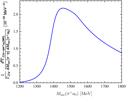
Figure 5: $\frac{1}{\Gamma_{J/\psi}}\,\frac{{\rm d}^{2}\Gamma_{J/\psi\to\phi\pi^{+}a_{0}(980)}}{{\rm d}M_{\rm inv}(\pi^{-}\eta)\;{\rm d}M_{\rm inv}(\pi^{+}a_{0})}$ as a function of $M_{\rm inv}(\pi^{+}a_{0})$ when fixing $M_{\rm inv}(\pi^{-}\eta)=m_{a_{0}}$.

We see a clear peak around $M_{\rm inv}(\pi^{+}a_{0})=1440\textrm{ MeV}$, coming from $|\tilde{t}^{\prime}_{\rm TS}|$ in Eq. (19). This is what one would observe in a devoted experiment with a bin of $1\textrm{ MeV}$ for $M_{\rm inv}(\pi^{+}a_{0})$, and $1\textrm{ MeV}$ for $M_{\rm inv}(\pi^{-}\eta)$. Obviously, the accumulation of events in bigger bins increases the statistics, as we shall see.

III.2 Fixing $M_{\rm inv}(\pi^{+}a_{0})=1416\,\textrm{ MeV}$

In Fig. 6, we now set $M_{\rm inv}(\pi^{+}a_{0})=1416\,\textrm{ MeV}$ and plot $\tilde{t}^{\prime}_{\rm TS}$ as a function of $M_{\rm inv}(\pi^{-}\eta)$.

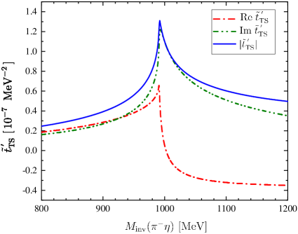
Figure 6: $\tilde{t}^{\prime}_{\rm TS}$ given by Eq. (26) as a function of $M_{\rm inv}(\pi^{-}\eta)$ when fixing $M_{\rm inv}(\pi^{+}a_{0})=1416\textrm{ MeV}$.

Once more, we display the real and imaginary parts of the amplitude, as well as its modulus. We see again that the imaginary part and the modulus delineate the shape of the $a_{0}(980)$ resonance. The real part changes sign at the peak of the $a_{0}(980)$, reflecting a typical resonance behaviour. It is interesting to see that even if the $a_{0}(980)$ appears as cusp, corresponding to a nearly missed bound state, or virtual state, it still exhibits the typical shape of a resonance amplitude. Such kind of behaviours for nearly missed bound states can be seen in other cases. For instance, in the $pd\to{{}^{3}\rm He}\,\eta$ reaction He3eta (see Fig. 8 of that work), the amplitude exhibits a resonance structure with a peak very close to and just below the ${{}^{3}\rm He}\,\eta$ threshold. However, there is no pole below threshold, and technically, no bound state.

In Fig. 7, we show again $\frac{1}{\Gamma_{J/\psi}}\,\frac{{\rm d}^{2}\Gamma_{J/\psi\to\phi\pi^{+}a_{0}(980)}}{{\rm d}M_{\rm inv}(\pi^{-}\eta)\;{\rm d}M_{\rm inv}(\pi^{+}a_{0})}$ as a function of $M_{\rm inv}(\pi^{-}\eta)$, fixing now $M_{\rm inv}(\pi^{+}a_{0})$ at the peak of the TS amplitude.

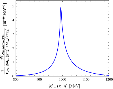
Figure 7: $\frac{1}{\Gamma_{J/\psi}}\,\frac{{\rm d}^{2}\Gamma_{J/\psi\to\phi\pi^{+}a_{0}(980)}}{{\rm d}M_{\rm inv}(\pi^{-}\eta)\;{\rm d}M_{\rm inv}(\pi^{+}a_{0})}$ as a function of $M_{\rm inv}(\pi^{-}\eta)$ when fixing $M_{\rm inv}(\pi^{+}a_{0})=1416\textrm{ MeV}$.

This comes from Eq. (19) and contains $|\tilde{t}^{\prime}_{\rm TS}|^{2}$ along with the phase space. The shape of the $a_{0}(980)$ resonance shows up as a clear cusp structure, as seen in recent experiments with high resolution Rubin ; midhalo ; besnew .

III.3 integrating $\frac{1}{\Gamma_{J/\psi}}\,\frac{{\rm d}^{2}\Gamma_{J/\psi\to\phi\pi^{+}a_{0}(980)}}{{\rm d}M_{\rm inv}(\pi^{-}\eta)\;{\rm d}M_{\rm inv}(\pi^{+}a_{0})}$ over $M_{\rm inv}(\pi^{-}\eta)$

Fig. 8 shows $\frac{1}{\Gamma_{J/\psi}}\,\frac{{\rm d}^{2}\Gamma_{J/\psi\to\phi\pi^{+}a_{0}(980)}}{{\rm d}M_{\rm inv}(\pi^{-}\eta)\;{\rm d}M_{\rm inv}(\pi^{+}a_{0})}$ as a function of $M_{\rm inv}(\pi^{+}a_{0})$, when integrating over $M_{\rm inv}(\pi^{-}\eta)$ in the ranges of $m_{a_{0}}\pm 10\textrm{ MeV}$, $m_{a_{0}}\pm 20\textrm{ MeV}$, $m_{a_{0}}\pm 50\textrm{ MeV}$ and $m_{a_{0}}\pm 100\textrm{ MeV}$, respectively.

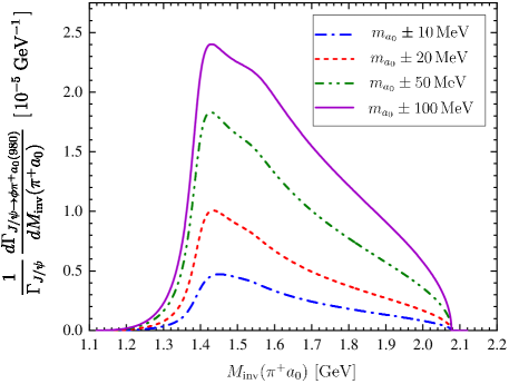
Figure 8: $\frac{1}{\Gamma_{J/\psi}}\,\frac{d^{2}\Gamma_{J/\psi\to\phi\pi^{+}a_{0}(980)}}{{\rm d}M_{\rm inv}(\pi^{-}\eta)\;{\rm d}M_{\rm inv}(\pi^{+}a_{0})}$ as a function of $M_{\rm inv}(\pi^{+}a_{0})$ when integrating over $M_{\rm inv}(\pi^{-}\eta)$ in the ranges: $m_{a_{0}}\pm 10\textrm{ MeV}$, $m_{a_{0}}\pm 20\textrm{ MeV}$, $m_{a_{0}}\pm 50\textrm{ MeV}$ and $m_{a_{0}}\pm 100\textrm{ MeV}$.

In all the cases, we observe a peak corresponding to the TS. By looking at Fig. 8, we can see that integrating the double mass distribution over $M_{\rm inv}(\pi^{-}\eta)$ within the range $m_{a_{0}}\pm 100\textrm{ MeV}$ accounts for the whole strength of the $a_{0}(980)$ resonance. And we interpret this as indicative of what should be observed in the experiments. The shape of the TS is clearly observed.

For the case where $M_{\rm inv}(\pi^{-}\eta)\in[m_{a_{0}}-100,m_{a_{0}}+100]\textrm{ MeV}$, integrating over $M_{\rm inv}(\pi^{+}a_{0})$ in the range $[m_{\pi^{+}}+m_{a_{0}},M_{J/\psi}-m_{\phi}]$ gives the branching ratio

$${\rm Br}(J/\psi\to\phi\pi^{+}a_{0})=1.07\times 10^{-5}.$$ (32)

This estimate is realistic, as the only unknown magnitude required to evaluate the diagrams of Figs. 2(a) and 2(c) is the $J/\psi\to\phi K^{*+}K^{-}$ amplitude, which we obtained from the experimental data. This branching ratio is not small, given the copious production of $J/\psi$ at BESIII, which allows to detect decays with branching fractions as small as $10^{-7}$ pdg . In view of this, we can only encourage the measurement of this reaction, which could also serve to clarify issues on the $J/\psi\to\pi^{0}\eta\phi\,(\phi\to K\bar{K})$ reaction besrecent and its interpretation in Ref. jingsakaiguo in terms of a TS.

IV Conclusions

We have conducted a study of the $J/\psi\to\phi\pi^{+}a_{0}(980)^{-}\;(a_{0}^{-}\to\pi^{-}\eta)$ decay, showing that it develops a triangle singularity at $M_{\rm inv}(\pi^{+}a_{0})$ of about $1420\,\rm MeV$. The reaction proposed is motivated by the recent measurement at BESIII of the $J/\psi\to\eta\pi^{0}\phi\;(\phi\to K\bar{K})$ reaction besrecent , that according to the work of Ref. jingsakaiguo also develops a triangle singularity, however, blurred by the tree level competing mechanisms and their interconnection with the Coleman Norton theorem. In the reaction proposed there is no tree level competing mechanism and then the TS appearing can be clearly interpreted. We evaluate the mass distributions in terms of $M_{\rm inv}(\pi^{-}\eta)$ and $M_{\rm inv}(\pi^{+}a_{0})$. In the $\pi^{-}\eta$ mass distribution we see a clear cusp structure, as observed in recent high statistics experiments, and in the $\pi^{+}a_{0}$ mass distribution we observe the TS peak around $M_{\rm inv}(\pi^{+}a_{0})=1420\,\rm MeV$. By taking information for the needed $J/\psi\to\eta K^{*}\bar{K}$ amplitude from experiment, we are able to determine absolute rates for the reaction. Integrating the double mass distribution in the range of the $a_{0}(980)$ mass and in the range of the $\pi^{+}a_{0}$ mass distribution, we predict a branching ratio for the reaction of the order of $10^{-5}$. Given the present rates of $J/\psi$ production at BESIII, where branching ratios of $10^{-7}$ can be measured, we advocate for the measurement of this reaction, that apart from showing a new example of a TS can also shed light on the interpretation of the recent BESIII measurements of the $J/\psi\to\eta\pi^{0}\phi\;(\phi\to K\bar{K})$ reaction.

- (1) R. Karplus, C. M. Sommerfield and E. H. Wichmann, Phys. Rev. 111, 1187-1190 (1958)
- (2) L. D. Landau, Nucl. Phys. 13, no.1, 181-192 (1959)
- (3) S. Coleman and R. E. Norton, Nuovo Cim. 38, 438-442 (1965)
- (4) C. Adolph et al. [COMPASS], Phys. Rev. Lett. 115, no.8, 082001 (2015)
- (5) X. H. Liu, M. Oka and Q. Zhao, Phys. Lett. B 753, 297-302 (2016)
- (6) M. Mikhasenko, B. Ketzer and A. Sarantsev, Phys. Rev. D 91, no.9, 094015 (2015)
- (7) F. Aceti, L. R. Dai and E. Oset, Phys. Rev. D 94, no.9, 096015 (2016)
- (8) G. D. Alexeev et al. [COMPASS], Phys. Rev. Lett. 127, no.8, 082501 (2021)
- (9) M. Ablikim et al. [BESIII], Phys. Rev. Lett. 108, 182001 (2012)
- (10) J. J. Wu, X. H. Liu, Q. Zhao and B. S. Zou, Phys. Rev. Lett. 108, 081803 (2012)
- (11) F. Aceti, W. H. Liang, E. Oset, J. J. Wu and B. S. Zou, Phys. Rev. D 86, 114007 (2012)
- (12) X. G. Wu, J. J. Wu, Q. Zhao and B. S. Zou, Phys. Rev. D 87, no.1, 014023 (2013)
- (13) C. Richard-Serre, W. Hirt, D. F. Measday, E. G. Michaelis, M. J. M. Saltmarsh and P. Skarek, Nucl. Phys. B 20, 413-440 (1970)
- (14) Said data base website. https://gwdac.phys.gwu.edu/
- (15) N. Ikeno, R. Molina and E. Oset, Phys. Rev. C 104, no.1, 014614 (2021)
- (16) H. J. Jing, S. Sakai, F. K. Guo and B. S. Zou, Phys. Rev. D 100, no.11, 114010 (2019)
- (17) S. Sakai, E. Oset and W. H. Liang, Phys. Rev. D 96, no.7, 074025 (2017)
- (18) W. H. Liang, S. Sakai, J. J. Xie and E. Oset, Chin. Phys. C 42, no.4, 044101 (2018)
- (19) F. K. Guo, X. H. Liu and S. Sakai, Prog. Part. Nucl. Phys. 112, 103757 (2020)
- (20) M. Bayar, F. Aceti, F. K. Guo and E. Oset, Phys. Rev. D 94, no.7, 074039 (2016)
- (21) M. Ablikim et al. [BESIII], [arXiv:2311.07043 [hep-ex]].
- (22) C. Schmid, “Final-State Interactions and the Simulation of Resonances,” Phys. Rev. 154, no.5, 1363 (1967)
- (23) V. R. Debastiani, S. Sakai and E. Oset, Eur. Phys. J. C 79, no.1, 69 (2019)
- (24) J. A. Oller and E. Oset, Nucl. Phys. A 620, 438-456 (1997) [erratum: Nucl. Phys. A 652, 407-409 (1999)]
- (25) N. Kaiser, Eur. Phys. J. A 3, 307-309 (1998)
- (26) V. E. Markushin, Eur. Phys. J. A 8, 389-399 (2000)
- (27) J. Nieves and E. Ruiz Arriola, Phys. Lett. B 455, 30-38 (1999)
- (28) R. L. Workman et al. [Particle Data Group], PTEP 2022, 083C01 (2022)
- (29) N. Ikeno, J. M. Dias, W. H. Liang and E. Oset, Phys. Rev. D 100, no.11, 114011 (2019)
- (30) S. Sakai, E. Oset and A. Ramos, Eur. Phys. J. A 54, no.1, 10 (2018)
- (31) D. Gamermann, J. Nieves, E. Oset and E. Ruiz Arriola, Phys. Rev. D 81, 014029 (2010)
- (32) J. X. Lin, J. T. Li, S. J. Jiang, W. H. Liang and E. Oset, Eur. Phys. J. C 81, no.11, 1017 (2021)
- (33) A. Bramon, A. Grau and G. Pancheri, Phys. Lett. B 283, 416-420 (1992)
- (34) R. Pavao, S. Sakai and E. Oset, Eur. Phys. J. C 77, no.9, 599 (2017).
- (35) E. Oset and L. Roca, Phys. Lett. B 782, 332-338 (2018).
- (36) L. R. Dai, Q. X. Yu and E. Oset, Phys. Rev. D 99, no.1, 016021 (2019).
- (37) W. H. Liang, H. X. Chen, E. Oset and E. Wang, Eur. Phys. J. C 79, no.5, 411 (2019).
- (38) F. K. Guo, X. H. Liu and S. Sakai, Prog. Part. Nucl. Phys. 112, 103757 (2020).
- (39) J. J. Xie, W. H. Liang, E. Oset, P. Moskal, M. Skurzok and C. Wilkin, Phys. Rev. C 95, no.1, 015202 (2017).
- (40) P. Rubin et al. [CLEO], Phys. Rev. Lett. 93, 111801 (2004).
- (41) M. Ablikim et al. [BESIII], Phys. Rev. D 95, no.3, 032002 (2017).
- (42) M. Ablikim et al. [BESIII], [arXiv:2309.05760 [hep-ex]].