Willmore-type variational problem for foliated hypersurfaces

Abstract

We study new Willmore-type variational problem for a hypersurface $M$ in $\mathbb{R}^{n+1}$ equipped with an $s$-dimensional foliation ${\cal F}$. Its general version is the Reilly-type functional $WF_{n,s}=\int_{M}F(\sigma^{\cal F}_{1},\ldots,\sigma^{\cal F}_{s})\,{\rm d}V$, where $\sigma^{\cal F}_{i}$ are elementary symmetric functions of the eigenvalues of the second fundamental form restricted on the leaves of $\cal F$. The first and second variations of such functionals are calculated, conformal invariance of some of $WF_{n,s}$ is also shown. The Euler-Lagrange equation for a critical hypersurface with a transversally harmonic (e.g., Riemannian) foliation $\cal F$ is found and examples with $s\leq 2$ and $s=n$ are considered. Critical hypersurfaces of revolution are found, and it is shown that they are a local minimum for special variations.

Keywords: hypersurface, Euclidean space, foliation, second fundamental form, mean curvature, Willmore’s type functional, Euler-Lagrange equations, conformal invariant

Mathematics Subject Classifications (2010) 53C12; 53C15; 53C42

1 Introduction

Many authors, e.g., [3, 4, 8, 10, 15, 16], were looking for an immersion $\phi:M^{n}\to\bar{M}^{n+1}$ of a smooth manifold $M^{n}\ (n\geq 2)$ into a Riemannian manifold $(\bar{M},\bar{g})$, in particular, Euclidean space $\mathbb{R}^{n+1}$, which is a critical point of the following functionals for compactly supported variations of $\phi$:

$$W_{n,p}=\int_{M}H^{p}\,{\rm d}V,\qquad J_{n,p}=\int_{M}\|{h}\,\|^{p}\,{\rm d}V.$$ (1)

Here, ${h}$ is the scalar second fundamental form of $\phi(M)$, ${H}=\frac{1}{n}\operatorname{trace}_{g}{h}$ is the mean curvature, ${\rm d}V$ is the volume form of the induced metric $g$ on $M$, and $p>0$. These functionals measure how much $\phi(M)$ differs from a minimal hypersurface ($H=0$) or a totally geodesic hypersurface ($h=0$). The actions (1) are a particular case of functionals $WF_{n}=\int_{M}F(H)\,{\rm d}V$ and $JF_{n}=\int_{M}F(\|h\|)\,{\rm d}V$, where $F$ is a $C^{3}$-regular function of one variable, e.g., [2, 6, 7, 9]. For a closed oriented smooth hypersurface $M^{n}$ in ${\mathbb{R}}^{n+1}$, we get $W_{n,n}\geq C_{n}$, where $C_{n}=\frac{2\pi^{(n+1)/2}}{\Gamma((n+1)/2)}$ is the area of the unit $n$-sphere; the equality $W_{n,n}=C_{n}$ holds if and only if $M^{n}$ is embedded as a hypersphere, see [3].

Variational problems for (1) were first posed by Thomas Willmore in [15] for $W_{2,2}$, which belongs to conformal geometry. The Euler-Lagrange equation for $W_{2,2}$ is the well known elliptic PDE

$$\Delta H+2\,H(H^{2}-K)=0,$$ (2)

where $\Delta$ is the Laplacian and $K$ – the gaussian curvature of $M^{2}$. Solutions of (2) are called Willmore surfaces. An important class of Willmore surfaces in $\mathbb{R}^{3}$ arise as the stereographic projection of minimal surfaces in the 3-sphere. By Lawson’s theorem, any compact orientable surface can be minimally embedded in the 3-sphere. For a closed orientable surface $M$ in $\mathbb{R}^{3}$, the inequality $W_{2,2}\geq C_{2}=4\pi$ holds with the equality for round spheres. If $M^{2}$ is a torus in $\mathbb{R}^{3}$, then, according the Willmore conjecture proven by F.C. Marques and A. Neves in [10], we have $W_{2,2}\geq 2\,\pi^{2}$; the equality holds if and only if the generating curve is a circle and the ratio of radii is $\frac{1}{\sqrt{2}}$. Willmore surfaces have applications in biophysics, materials science, architecture, etc., e.g., [14].

R. Reilly [12] and some mathematicians studied variations of more general functionals than (1):

$$WF_{n}=\int_{M}F(\sigma_{1},\ldots,\sigma_{n})\,{\rm d}V,\qquad JF_{n}=\int_{M}F(\tau_{1},\ldots,\tau_{n})\,{\rm d}V,$$ (3)

where $F\in C^{3}(\mathbb{R}^{n})$. The elementary symmetric functions $\sigma_{r}=\sum_{i_{1}<\ldots<i_{r}}k_{i_{1}}\ldots k_{i_{r}}\ (0\leq r\leq n)$ of the principal curvatures $k_{i}$ satisfy the equality $\sum\nolimits_{\,r=0}^{\,n}\sigma_{r}t^{r}=\det({\rm id}_{\,TM}+tA)$, where $A$ is the Weingarten operator, i.e., $g(AX,Y)=h(X,Y)$. The power sums of the principal curvatures, $\tau_{i}=k_{1}^{i}+\ldots+k_{n}^{i}={\rm trace}\,A^{i}$, can be expressed as polynomials of $\sigma_{r}$ using the Newton formulas, e.g., [13]. For example, $\sigma_{0}=1$, $\tau_{1}=\sigma_{1}=nH$, $\sigma_{n}=\det A$, $\tau_{2}=\|h\|^{2}$ and $2\,\sigma_{2}=\tau_{1}^{2}-\tau_{2}$. The $r$-th ($r\leq n$) order Willmore functional, introduced by Z. Guo in [6],

$$W^{\rm conf}_{n,r}=\int_{M}Q_{\,r}^{\,n/r}\,{\rm d}V,\quad Q_{r}=\sum\nolimits_{j=0}^{r}(-1)^{j+1}C^{j}_{r}S_{1}^{r-j}S_{j},$$ (4)

is a special case of (3), invariant under conformal group of $(\bar{M},\bar{g})$ and vanishing on totally umbilical hypersurfaces. Here, $S_{r}=\sigma_{r}/C^{r}_{n}$ (where $C^{r}_{n}=\frac{n!}{r!(n-r)!}$ is a binomial coefficient) is the $r$-th mean curvature function of a hypersurface. In particular, $Q_{2}=S_{1}^{2}-S_{2}=\frac{1}{n^{2}(n-1)}\,((n-1)\sigma_{1}^{2}-2\,n\,\sigma_{2})$. Examples of hypersurfaces in $\mathbb{R}^{n+1}$ that are critical for (4) are given in [7, 9].

An interesting problem is the generalization of the Willmore functional to submanifolds with additional structures, such as foliations or almost products. Let $M^{n}\ (n\geq 2)$ equipped with an $s$-dimensional $(1\leq s\leq n)$ foliation ${\cal F}$ be immersed into a Riemannian manifold $(\bar{M},\bar{g})$. Let $h_{\cal F}$ be the restriction of the second fundamental form of $M$ on the leaves of ${\cal F}$. Denote by $\tau^{\cal F}_{i}\ (1\leq i\leq s)$ the power sums, $\sigma^{\cal F}_{r}\ (1\leq r\leq s)$ elementary symmetric functions of the eigenvalues $k^{\cal F}_{1}\leq\ldots\leq k^{\cal F}_{s}$ of $h_{\cal F}$, and set $S^{\cal F}_{r}=\sigma^{\cal F}_{r}/C^{r}_{s}$. We have $\tau^{\cal F}_{1}=\sigma^{\cal F}_{1}=sH_{\cal F}=\operatorname{trace}_{g}h_{\cal F}$, $\tau^{\cal F}_{2}=\|h_{\cal F}\|^{2}$, $(\tau^{\cal F}_{1})^{2}-\tau^{\cal F}_{2}=2\,\sigma^{\cal F}_{2}$, etc. For foliation theory we refer to [5], the extrinsic geometry of foliations was developed in [13]. We study Reilly-type functionals for compactly supported variations of $(M^{n},{\cal F})$ immersed in $\mathbb{R}^{n+1}$:

$$WF_{n,s}=\int_{M}F(\sigma^{\cal F}_{1},\ldots,\sigma^{\cal F}_{s})\,{\rm d}V,\qquad JF_{n,s}=\int_{M}F(\tau^{\cal F}_{1},\ldots,\tau^{\cal F}_{s})\,{\rm d}V,$$ (5)

which for $s=n$ reduce to (3). For $F=(\sigma_{1}^{\cal F}/s)^{p}$ and $F=(\tau_{2}^{\cal F})^{p/2}$, the actions (5) read as

$$W_{n,p,s}=\int_{M}{H}_{\cal F}^{p}\,{\rm d}V,\qquad J_{n,p,s}=\int_{M}\|h_{\cal F}\|^{p}\,{\rm d}V,$$ (6)

which reduce to (1) for $s=n$.

Remark 1.

A foliated hypersurface in $\mathbb{R}^{n+1}$, whose leaves $\{L\}$ are minimal submanifolds in $\mathbb{R}^{n+1}$ is an example of a minimizer for (6)₁ with even $p$. A foliated hypersurface in $\mathbb{R}^{n+1}$ with an asymptotic distribution $T{\cal F}$ (in particular, a ruled hypersurface) is a minimizer for (6)₂. It is interesting to find critical hypersurfaces for actions (6) with ${H}_{\cal F}\neq 0$ or $h_{\cal F}\neq 0$ on an open dense set of $M$.

The following special case of (5) is invariant under conformal group of $(\bar{M},\bar{g})$, see Theorem 1:

$$W^{\rm conf}_{n,s,r}=\int_{M}(Q^{\cal F}_{r})^{n/r}\,{\rm d}V,\quad Q^{\cal F}_{r}=\sum\nolimits_{j=0}^{r}(-1)^{j+1}C^{j}_{r}(S^{\cal F}_{1})^{r-j}S^{\cal F}_{j},\quad r\leq s,$$ (7)

and reduces to (4) for $s=n$. Note that $Q^{\cal F}_{2}=(S^{\cal F}_{1})^{2}-S^{\cal F}_{2}=\frac{1}{s^{2}(s-1)}\,((s-1)(\sigma^{\cal F}_{1})^{2}-2s\,\sigma^{\cal F}_{2})$ and $Q^{\cal F}_{r}=0$ if $k^{\cal F}_{1}=\ldots=k^{\cal F}_{s}$, e.g., for hypersurfaces of revolution in $\mathbb{R}^{n+1}$ foliated by parallels.

We hope that foliated hypersurfaces, which are local minima for (5), will be useful for natural sciences and technology related to layered (laminated) non-isotropic materials.

The paper is organized as follows. Section 2 contains some lemmas (proved in Sect. 5) that help us calculate variations of Reilly-type functionals on foliated hypersurfaces in $\mathbb{R}^{n+1}$. In Section 3, conformal invariance of (7) is shown, the first variations of the functionals (5)–(7) are found, and the corresponding Euler-Lagrange equations for the case of transversally harmonic (for example, Riemannian) foliation are obtained. Then the second variations on critical hypersurfaces of some Willmore type functionals are calculated. In Section 4, applications to hypersurfaces with low-dimensional foliations are given, the critical hypersurfaces of revolution for the actions (6) are presented, and it is shown that they are a local minimum for special variations.

2 Auxiliary results

Let ${\bf r}:M^{n}\to\mathbb{R}^{n+1}$ be an immersion of a manifold $M$ into $\mathbb{R}^{n+1}$ with Euclidean metric $\bar{g}$ and the Levi-Civita connection $\bar{\nabla}$. We identify $M$ with its image ${\bf r}(M)$ and restrict our calculations to a relatively compact neighborhood $U\subset M$ with induced metric $g=\langle\cdot\,,\cdot\rangle$ and normal coordinates $(x^{1},\ldots,x^{n})$ centered at a point $x\in M$. Thus, $g_{ij}=\delta_{ij}$ (the Kronecker symbol) and $\Gamma^{k}_{ij}=0$ at $x$. Differentiation of a function $f$ (or a tensor) with respect to the variable $x^{i}$ will be denoted by $f_{i}$.

Let $\partial_{i}=\partial/\partial x^{i}$ be the coordinate vector fields on $U$. So, the vectors ${\bf r}_{i}=\bar{\nabla}_{\partial_{i}}{\bf r}$ form a local coordinate basis for the tangent bundle $TM$ along $U$, and we get $g=g_{ij}\,dx^{i}\,dx^{j}$, where $g_{ij}=\bar{g}({\bf r}_{i},{\bf r}_{j})=\langle{\bf r}_{i},{\bf r}_{j}\rangle$ and Einstein summation rule is used. Let ${\bf N}$ be a unit normal vector field to $M$ on $U$. The vectors ${\bf N}_{i}=\bar{\nabla}_{\partial_{i}}{\bf N}$ belong to the tangent space $T_{x}M$, i.e., $\langle{\bf N}_{i},{\bf N}\rangle=0$.

Let ${h}$ be the scalar second fundamental form of $M$ with respect to unit normal ${\bf N}$, $A=-\bar{\nabla}\,{\bf N}$ the Weingarten operator and ${H}=\frac{1}{n}\operatorname{trace}_{g}{h}$ the mean curvature. Denote by $h^{j}$ the symmetric tensor dual to $A^{j}$, i.e., $h^{j}(X,Y)=\langle A^{j}X,Y\rangle$. For example, ${h}^{2}=g^{kl}h_{li}h_{kj}\,dx^{i}dx^{j}={h}^{k}_{i}h_{kj}\,dx^{i}dx^{j}$.

Consider a one-parameter family of hypersurfaces ${\bf r}_{t}={\bf r}+t\,u\,{\bf N}\ (|t|<1)$. We get a variation $\delta\,{\bf r}=u\,{\bf N}$, where $\delta=(d/dt)|_{\,t=0}$ is the variational derivative operator, and $u:U\to\mathbb{R}$ is a smooth function supported on relatively compact neighborhood $U$. Obviously, $(\delta\,{\bf r})_{i}=u_{i}\,{\bf N}+u\,{\bf N}_{i}$. The Hessian of a function $u$ is a (0,2)-tensor $({\rm Hess}_{\,u})(X,Y)=X(Y(u))-(\nabla_{X}\,Y)u=(u_{ij}-\Gamma^{k}_{ij}u_{k})dx^{i}dx^{j}$, see [11, pp. 48, 69]. The Laplacian is $\Delta u=\operatorname{trace}_{g}\,{\rm Hess}_{\,u}=g^{ij}u_{ij}$. Note that $\langle g,{\rm Hess}_{\,u}\rangle=\Delta\,u$. The divergence of a vector field $X=X^{i}\partial_{i}$ on $M$ is ${\rm div}\,X=\nabla_{i}X^{i}$.

Lemma 1 (see [8] for $n=2$).

The following evolution equations are true:

$$\delta\,g_{ij}=-2\,u\,h_{ij},$$ (8)

$$\delta\,g^{ij}=2\,u\,h^{ij},$$ (9)

$$\delta\,h_{ij}=u_{ij}-u{h}^{l}_{i}\,h_{jl}\ \Leftrightarrow\ \delta\,h={\rm Hess}_{\,u}-u\,h^{2},$$ (10)

$$\delta\,\|h\|^{2}=2\,\langle h,\ u{h}^{2}+{\rm Hess}_{\,u}\rangle,$$ (11)

$$\delta(nH)=\Delta\,u+u\,\|h\|^{2},$$ (12)

$$\delta\,{\rm d}V=-n\,uH\,{\rm d}V.$$ (13)

We carry out further calculations for a foliated hypersurface $(M,{\cal F})$ and a foliated neighborhood $U\subset M$ with normal coordinates $(x^{1},\ldots,x^{n})$ adapted to ${\cal F}$, i.e., $(x^{1},\ldots,x^{s})$ are variables along the leaves, see [5]. Let $\nabla^{\cal F}:TM\times T{\cal F}\to T{\cal F}$ be the induced Levi-Civita connection on the subbundle $T{\cal F}\subset TM$ and on the leaves of ${\cal F}$. The leafwise Laplacian on functions is $\Delta_{\,\cal F}=\operatorname{trace}_{g}\,{\rm Hess}^{\cal F}={\rm div}_{\cal F}\circ\nabla^{\,\cal F}$, where ${\rm Hess}^{\cal F}$ is the Hessian on the leaves of $\cal F$. Let $P:TM\to T{\cal F}$ be the orthoprojector, thus $P^{2}=P$ and $P$ is self-adjoint. For $h_{\cal F}$ and its dual self-adjoint operator $A_{\cal F}$ we can write $h_{\cal F}(X,Y)=h(PX,PY)\ (X,Y\in\mathfrak{X}_{M})$ and $A_{\cal F}=PAP$. Let $h_{\cal F}^{j}$ be the symmetric tensor dual to $A_{\cal F}^{j}$, i.e., $h_{\cal F}^{j}(X,Y)=\langle A_{\cal F}^{j}X,Y\rangle$. The symmetric tensor $h_{\rm mix}$ is given by

$$h_{\rm mix}(X,Y)=\frac{1}{2}\,\big{(}h(PX,Y)+h(X,PY)\big{)}-h(PX,PY),\quad X,Y\in\mathfrak{X}_{M}.$$

We have $\langle h_{\cal F},h_{\rm mix}\rangle=0$. The equality $h_{\rm mix}=0$ means that $PA=AP$, i.e., $T{\cal F}$ is an invariant subbundle for $A$. Let $h_{\cal F^{\perp}}$ be the restriction of $h$ on the normal distribution to ${\cal F}$ in $M$, then $h_{\cal F^{\perp}}^{2}=g^{\gamma\epsilon}h_{\alpha\gamma}h_{\alpha\epsilon}dx^{\alpha}dx^{\beta}$, where $s<\alpha,\beta,\gamma,\epsilon\leq n$. Define symmetric tensors $h_{\rm mix}^{2}=g^{\alpha\beta}h_{\alpha i}h_{\beta j}dx^{i}dx^{j}+g^{ij}h_{\alpha i}h_{\beta j}\,dx^{\alpha}dx^{\beta}$ and ${\rm Hess}^{\,\rm mix}_{\,u}=g^{ij}g^{\alpha\beta}u_{i\alpha}\,dx^{j}dx^{\beta}$, where $1\leq i,j\leq s$ and $s<\alpha,\beta,\gamma,\epsilon\leq n$. Let $A_{\,\rm mix}$ be the (1,1)-tensor dual to $h_{\rm mix}$, then $A^{2}_{\,\rm mix}$ is dual to $h^{2}_{\,\rm mix}$.

The Newton transformations $T_{r}(A_{\cal F})$ of $A_{\cal F}$ are defined inductively or explicitly by, e.g. [13],

$$T_{0}(A_{\cal F}) = {\rm id}_{\,T\cal F},\quad T_{r}(A_{\cal F})=\sigma^{\cal F}_{r}\,{\rm id}_{\,T\cal F}-A_{\cal F}\,T_{r-1}(A_{\cal F})\quad(0<r\leq s),$$

$$T_{r}(A_{\cal F}) = \sum\nolimits_{j=0}^{r}(-1)^{j}\sigma^{\cal F}_{r-j}\,A_{\cal F}^{j}=\sigma^{\cal F}_{r}\,{\rm id}_{\,T\cal F}-\sigma^{\cal F}_{r-1}\,A_{\cal F}+\ldots+(-1)^{r}A_{\cal F}^{\,r}.$$

For example, $T_{1}(A_{\cal F})=\sigma^{\cal F}_{1}\,{\rm id}_{\,T\cal F}-A_{\cal F}$ and $T_{s}(A_{\cal F})=0$ and the following equalities are true:

$$\operatorname{trace}T_{r}(A_{\cal F})=(s-r)\,\sigma^{\cal F}_{r},\quad\operatorname{trace}(A_{\cal F}\,T_{r}(A_{\cal F}))=(r+1)\,\sigma^{\cal F}_{r+1},$$

$$\operatorname{trace}(A_{\cal F}^{2}\,T_{r}(A_{\cal F}))=\sigma^{\cal F}_{1}\sigma^{\cal F}_{r+1}-(r+2)\,\sigma^{\cal F}_{r+2}.$$ (14)

The “musical” isomorphism $\sharp:T^{*}M\to TM$ is used for tensors, e.g., $h^{\sharp}=A$, and for $(0,2)$-tensors $B$ and $C$ we have $\langle B,C\rangle=\operatorname{trace}(B^{\sharp}C^{\sharp})=\langle B^{\sharp},C^{\sharp}\rangle$.

Lemma 2.

The variations of $\tau^{\cal F}_{i}$ and $\sigma^{\cal F}_{r}$ are the following:

$$\frac{1}{i}\,\delta\,\tau^{\cal F}_{i}=\langle h_{\cal F}^{i-1},{\rm Hess}^{\cal F}_{u}\rangle+u\,(\tau^{\cal F}_{i+1}+\langle h_{\cal F}^{i-1},h^{2}_{\,\rm mix}\rangle),$$

$$\delta\,\sigma^{\cal F}_{r}=\langle T_{r-1}(A_{\cal F}),{\rm Hess}^{\cal F\sharp}_{u}\rangle+u\big{(}\sigma^{\cal F}_{1}\sigma^{\cal F}_{r-1}-(r+1)\,\sigma^{\cal F}_{r+1}+\langle T_{r-1}(A_{\cal F}),\,A_{\,\rm mix}^{2}\rangle\big{)}.$$ (15)

Proof.

By (10), we obtain $\delta A_{\cal F}={\rm Hess}^{\cal F\sharp}_{u}+u(A_{\cal F}^{2}+A_{\,\rm mix}^{2})$. Using this, (2) and the the following variations of $\tau^{\cal F}_{i}$ and $\sigma^{\cal F}_{r}$, see [13, Sect. 1.5.3]:

$$\delta\,\tau^{\cal F}_{i}=i\operatorname{trace}(A_{\cal F}^{i-1}\delta A_{\cal F}),\quad\delta\,\sigma^{\cal F}_{r}=\operatorname{trace}(T_{r-1}(A_{\cal F})\,\delta A_{\cal F}),$$

we get (2). ∎

Lemma 3.

The following evolution equations are true:

$$\delta\,(s\,{H}_{\cal F})=\Delta_{\,\cal F}\,u+u\,(\|h_{\cal F}\|^{2}-\|h_{\rm mix}\|^{2}),$$ (16)

$$\delta\,\|h_{\cal F}\|^{2}=2\,\langle h_{\cal F},\ u\,(h_{\cal F}^{2}+h_{\rm mix}^{2})+{\rm Hess}^{\,\cal F}_{\,u}\rangle,$$ (17)

$$\delta\,\|h_{\rm mix}\|^{2}=u\,\langle h_{\cal F}+h_{\cal F^{\perp}},h_{\rm mix}^{2}\rangle+2\,\langle h_{\rm mix},{\rm Hess}^{\,\rm mix}_{\,u}\rangle.$$ (18)

For any smooth function $f:M\times\mathbb{R}\to\mathbb{R}$ the following evolution is true:

$$\delta\,(\Delta_{\,\cal F}f)=\Delta_{\,\cal F}\dot{f}+2\,u\langle h_{\cal F},{\rm Hess}^{\,\cal F}_{f}\rangle{+}su\langle\nabla^{\cal F}H_{\cal F},\nabla^{\cal F}f\rangle{+}2\,h(\nabla^{\,\cal F}u,\nabla^{\cal F}f){-}sH_{\cal F}\langle\nabla^{\cal F}u,\nabla^{\cal F}f\rangle.$$ (19)

Remark 2.

The equations (16)–(17) can be deduced from Lemma 2, but we will prove them in Section 5. To find the second variation of the functionals (5) we need also the variation $\delta\,\langle h,{\rm Hess}^{\,\cal F}_{\,u}\rangle$, but we omit this calculation and consider the second variation of the functionals (6) only.

The following property helps to find the Euler-Lagrange equations using first variation of (3)–(6):

$$({\rm div}\,P)\circ P=0.$$ (20)

Here, $({\rm div}\,P)X=\sum\nolimits_{\,i=1}^{n}\langle(\nabla_{e_{i}}P)X,e_{i}\rangle$, where $e_{1},\ldots,e_{n}$ is a local orthonormal basis on $M$. Note that Riemannian foliations (and the leaves of twisted products, e.g., [13]) satisfy (20).

Lemma 4.

A foliated Riemannian manifold $(M,g,{\cal F})$ satisfies (20) if and only if ${\cal F}$ is transversally harmonic, i.e., the normal distribution has zero mean curvature.

Proof.

Using a local orthonormal frame on $M$ such that $e_{i}\in T{\cal F}\ (1\leq i\leq s)$, we calculate:

$$({\rm div}\,P)(PX)=\sum\nolimits_{\,i=1}^{n}\langle(\nabla_{e_{i}}P)(PX),e_{i}\rangle=\sum\nolimits_{\,i=1}^{n}\big{\{}\langle\nabla_{e_{i}}(P^{2}X),e_{i}\rangle-\langle P\nabla_{e_{i}}(PX),e_{i}\rangle\big{\}}$$

$$=\sum\nolimits_{\,i=1}^{n}\big{\{}\langle\nabla_{e_{i}}(PX),e_{i}\rangle-\langle\nabla_{e_{i}}(PX),Pe_{i}\rangle\big{\}}=\sum\nolimits_{\,i>s}\langle\nabla_{e_{i}}(PX),e_{i}\rangle=-\langle X,(n-s)H^{\perp}\rangle,$$

where $(n-s)H^{\perp}=P\sum_{\,i>s}\nabla_{e_{i}}e_{i}$ is the mean curvature vector of $(T{\cal F})^{\perp}$ and $X\in\mathfrak{X}_{M}$. ∎

For any 2-tensor $B$ on $M$ define the adjoint of the covariant derivative $\nabla^{*}B=-\sum_{\,i}(\nabla_{i}\,B)(e_{i},\cdot)$, see [11, p. 59]. We have the formula $\int_{M}\langle B,\nabla B^{\prime}\rangle\,{\rm d}V=\int_{M}\langle\nabla^{*}B,B^{\prime}\rangle\,{\rm d}V$, see [11, p. 60]; thus,

$$\int_{M}\langle B,{\rm Hess}_{\,u}\rangle\,{\rm d}V=\int_{M}\langle B,\nabla(\nabla u)\rangle\,{\rm d}V=\int_{M}\langle\nabla^{*}B,\nabla u\rangle\,{\rm d}V=\int_{M}u\,(\nabla^{*})^{2}(B)\,{\rm d}V.$$ (21)

The next lemma generalizes (21) and the well known Green’s formula, e.g., [11, p. 75].

Lemma 5.

If a foliated Riemannian manifold $(M,g,{\cal F})$ satisfies (20), then the following formulas are valid for any compactly supported functions $u,f$ and 2-tensor $B$:

$$\int_{M}f(\Delta_{\,\cal F}\,u)\,{\rm d}V=\int_{M}u(\Delta_{\,\cal F}\,f)\,{\rm d}V,$$ (22)

$$\int_{M}\langle B,{\rm Hess}^{\cal F}_{\,u}\rangle\,{\rm d}V=\int_{M}u\,(\nabla^{{\cal F}*})^{2}(B)\,{\rm d}V.$$ (23)

3 Main results

In Sect.3.1, we find the Euler-Lagrange equations (and first variations) for the functionals (5)–(7), and in Sect. 3.2 we find the second variations of (5) and (6). First we check the conformity of (7).

Theorem 1.

The functional $W^{\rm conf}_{n,s,r}$ is a conformal invariant of a foliated hypersurface $(M,{\cal F})$ in a Riemannian manifold $(\bar{M},\bar{g})$.

Proof.

Define a new Riemannian metric on $\bar{M}$ by $\bar{g}^{c}=\mu^{2}\bar{g}$ for some positive function $\mu\in C^{3}(\bar{M})$. Then $g^{c}=\mu^{2}g$ is the new induced metric on $M$, thus, the new volume form of $M$ is ${\rm d}V^{c}=\mu^{n}\,{\rm d}V$. If $X$ is a $\bar{g}$-unit vector, then $X^{c}=X/\mu$ is a $g^{c}$-unit vector. By the well known formula for the Levi-Civita connection, e.g., [13, p. 14], we get

$$2\,\bar{\nabla}^{\,c}_{X}\,Y=2\,\bar{\nabla}_{X}\,Y+\mu^{-2}\big{(}X(\mu^{2})Y+Y(\mu^{2})X-\langle X,Y\rangle\bar{\nabla}\mu^{2}\big{)}.$$

By this with $X\in T{\cal F}$ and $Y={\bf N}^{\,c}$, the operators $A$ and $A^{c}$ are related by $A^{c}=\frac{1}{\mu}\big{(}A-\frac{1}{\mu}\langle\bar{\nabla}\mu,N\rangle\,{\rm id}_{\,T\cal F}\big{)}$, see also [13, Sect. 2.1.2.2]. By the above and $A_{\cal F}=PAP$, $A^{\,c}_{\cal F}=PA^{c}P$, we get

$$A_{\cal F}^{c}=\frac{1}{\mu}\big{(}A_{\cal F}-\frac{1}{\mu}\langle\bar{\nabla}\mu,N\rangle\,{\rm id}_{\,T\cal F}\big{)},\quad H_{\cal F}^{c}=\frac{1}{s}\operatorname{trace}A_{\cal F}^{c}=\frac{1}{\mu}\big{(}H_{\cal F}-\frac{1}{\mu}\langle\bar{\nabla}\mu,N\rangle\big{)}.$$

Set $B_{\cal F}=H_{\cal F}\,{\rm id}_{\,T\cal F}-A_{\cal F}$. Let $\lambda^{B}_{i}$ be the eigenvalues of $B_{\cal F}$ on ${\cal F}$ and $\sigma^{B}_{r}$ be elementary symmetric functions of $B_{\cal F}$. Obviously, $B_{\cal F}^{\,c}=\frac{1}{\mu}\,B_{\cal F}$ holds; hence, $\lambda^{B,c}_{i}=\frac{1}{\mu}\,\lambda^{B}_{i}$. One can show that $Q^{\cal F}_{r}=-\sigma^{B}_{r}/C^{s}_{r}$ is true, see [6, Lemma 2.1]. By the above, $\mu^{r}Q^{{\cal F},c}_{r}=Q^{\cal F}_{r}$ holds. Hence, $(Q^{\cal F}_{r})^{n/r}{\rm d}V$ is a conformal invariant of $(M,{\cal F})$ in $(\bar{M},\bar{g})$: $(Q^{{\cal F},c}_{r})^{n/r}{\rm d}V^{c}=(Q^{\cal F}_{r})^{n/r}{\rm d}V$. Note that if $A_{\cal F}$ is a conformal operator on $T{\cal F}$ (i.e., proportional to ${\rm id}_{\,T\cal F}$), then $B_{\cal F}=0$, hence, $Q^{\cal F}_{r}=0$. ∎

3.1 The first variation

We can state our main theorem.

Theorem 2.

If (20) is valid, then Euler-Lagrange equations for the functionals (5) are

$$\sum\nolimits_{\,r=1}^{s}\big{\{}(\nabla^{{\cal F}*})^{2}\big{(}F^{\prime}_{r}\cdot T_{r-1}(A_{\cal F})\big{)}+F^{\prime}_{r}\big{(}\sigma^{\cal F}_{1}\sigma^{\cal F}_{r-1}{-}(r+1)\sigma^{\cal F}_{r+1}{+}\langle T_{r-1}(A_{\cal F}),A_{\,\rm mix}^{2}\rangle\big{)}\big{\}}-nFH=0,$$

$$\sum\nolimits_{\,i=1}^{s}\frac{1}{i}\,\big{\{}(\nabla^{{\cal F}*})^{2}\big{(}F^{\prime}_{i}\cdot A_{\cal F}^{i-1}\big{)}+F^{\prime}_{i}\big{(}\tau^{\cal F}_{i+1}+\langle h_{\cal F}^{i-1},h^{2}_{\,\rm mix}\rangle\big{)}\big{\}}-nFH=0.$$ (24)

Proof.

Using (13), we get the following:

$$\delta\,WF_{n,s}=\int_{M}\delta\,(F(\sigma^{\cal F}_{1},\ldots,\sigma^{\cal F}_{s})\,{\rm d}V)=\int_{M}\Big{\{}\sum\nolimits_{r=1}^{s}F^{\prime}_{r}\cdot\delta\,\sigma^{\cal F}_{r}-n\,uFH\Big{\}}{\rm d}V,$$

$$\delta\,JF_{n,s}=\int_{M}\delta\,(F(\tau^{\cal F}_{1},\ldots,\tau^{\cal F}_{s})\,{\rm d}V)=\int_{M}\Big{\{}\sum\nolimits_{i=1}^{s}F^{\prime}_{i}\cdot\delta\,\tau^{\cal F}_{i}-n\,uFH\Big{\}}{\rm d}V.$$ (25)

From (3.1) and (2) we find the first variations of functionals (5):

$$\delta\,WF_{n,s}=\int_{M}\Big{\{}\sum\nolimits_{\,r=1}^{s}\langle F^{\prime}_{r}\cdot T_{r-1}(A_{\cal F}),{\rm Hess}^{\cal F\sharp}_{u}\rangle$$

$$\quad+u\sum\nolimits_{\,r=1}^{s}F^{\prime}_{r}\big{(}\sigma^{\cal F}_{1}\sigma^{\cal F}_{r-1}-(r+1)\sigma^{\cal F}_{r+1}+\langle T_{r-1}(A_{\cal F}),A_{\,\rm mix}^{2}\rangle\big{)}-n\,uFH\Big{\}}{\rm d}V,$$

$$\delta\,JF_{n,s}=\int_{M}\Big{\{}\sum\nolimits_{\,i=1}^{s}\frac{1}{i}\,F^{\prime}_{i}\big{(}\langle h_{\cal F}^{i-1},{\rm Hess}^{\cal F}_{u}\rangle+u\,(\tau^{\cal F}_{i+1}+\langle h_{\cal F}^{i-1},h^{2}_{\,\rm mix}\rangle)\big{)}-n\,uFH\Big{\}}{\rm d}V.$$ (26)

From (3.1), using (20) and (22), we obtain (2). ∎

Equations (27) and (28) of the next statement follow from Theorem 2, but we will prove them.

Corollary 1.

If (20) is valid, then the Euler-Lagrange equations for the functionals $W_{n,p,s},\,J_{n,p,s}$, see (6), and $W^{\rm conf}_{n,s,2}$, see (7), are, respectively, the following:

$$\Delta_{\,\cal F}\,({H}_{\cal F}^{p-1})+{H}_{\cal F}^{p-1}\big{(}\|h_{\cal F}\|^{2}-\|h_{\rm mix}\|^{2}-\frac{n\,s}{p}\,H{H}_{\cal F}\big{)}=0,$$ (27)

$$(\nabla^{{\cal F}*})^{2}(\|h_{\cal F}\|^{p-2}h_{\cal F})+\|h_{\cal F}\|^{p-2}\big{(}\langle h_{\cal F},\ h_{\cal F}^{2}+h_{\rm mix}^{2}\rangle-\frac{n}{p}\,\|h_{\cal F}\|^{2}\,H\big{)}=0,$$ (28)

$$\Delta_{\,\cal F}\,\big{(}(Q^{\cal F}_{2})^{n/2-1}\sigma^{\cal F}_{1}\big{)}-\frac{s}{s-1}\,(\nabla^{\cal F*})^{2}\big{(}(Q^{\cal F}_{2})^{n/2-1}T_{1}(A_{\cal F})\big{)}+\big{\{}\sigma^{\cal F}_{1}(\sigma^{\cal F}_{1}-2\,\sigma^{\cal F}_{2}+\|A_{\,\rm mix}\|^{2})$$

$$\quad-\frac{s}{s-1}\,(\sigma^{\cal F}_{1}\sigma^{\cal F}_{2}-3\,\sigma^{\cal F}_{3}+\langle T_{1}(A_{\cal F}),\,A_{\,\rm mix}^{2}\rangle)-s^{2}Q^{\cal F}_{2}H\big{\}}(Q^{\cal F}_{2})^{n/2-1}=0.$$ (29)

Proof.

a) Using (13), (16) and (17) we calculate the variation

$$\delta\,({H}_{\cal F}^{p}\,{\rm d}V) ={H}_{\cal F}^{p-1}\Big{\{}\frac{p}{s}\,\big{(}\Delta_{\,\cal F}\,u+u\,(\|h_{\cal F}\|^{2}-\|h_{\rm mix}\|^{2})\big{)}-nu{H}{H}_{\cal F}\Big{\}}{\rm d}V,$$

$$\delta\,(\|h_{\cal F}\|^{p}\,{\rm d}V)=\|h_{\cal F}\|^{p-2}\big{\{}p\,\langle h_{\cal F},\ u\,(h_{\cal F}^{2}+h_{\rm mix}^{2})+{\rm Hess}^{\,\cal F}_{\,u}\rangle-n\,u\,\|h_{\cal F}\|^{2}\,{H}\big{\}}{\rm d}V.$$

Hence, using (20), (22), (23) and (13), we find the first variation of the actions (6):

$$\delta\,W_{n,p,s} =\int_{M}\delta\,({H}_{\cal F}^{p}\,{\rm d}V)=\int_{M}{H}_{\cal F}^{p-1}\Big{\{}\frac{p}{s}\,\big{(}\Delta_{\,\cal F}\,u+u\,(\|h_{\cal F}\|^{2}-\|h_{\rm mix}\|^{2})\big{)}-n\,u\,{H}_{\cal F}H\Big{\}}{\rm d}V$$

$$=\frac{p}{s}\int_{M}u\Big{\{}\Delta_{\,\cal F}({H}_{\cal F}^{p-1})+{H}_{\cal F}^{p-1}\,\big{(}\|h_{\cal F}\|^{2}-\|h_{\rm mix}\|^{2}-\frac{n\,s}{p}\,{H}{H}_{\cal F}\big{)}\Big{\}}{\rm d}V,$$ (30)

$$\delta\,J_{n,p,s} =\int_{M}\|h_{\cal F}\|^{p-2}\Big{\{}p\,\langle h_{\cal F},\,u\,(h_{\cal F}^{2}+h_{\rm mix}^{2})+{\rm Hess}^{\,\cal F}_{\,u}\rangle-n\,u\,\|h_{\cal F}\|^{2}\,{H}\Big{\}}{\rm d}V$$

$$=\int_{M}u\Big{\{}p\,(\nabla^{{\cal F}*})^{2}(\|h_{\cal F}\|^{p-2}h_{\cal F})+p\,\|h_{\cal F}\|^{p-2}\big{(}\langle h_{\cal F},h_{\cal F}^{2}+h_{\rm mix}^{2}\rangle-n\,\|h_{\cal F}\|^{2}\,{H}\big{)}\Big{\}}{\rm d}V.$$ (31)

From (3.1) and (3.1) the Euler-Lagrange equations (27) and (28) follow. By (2)₂ we get

$$\delta\,\sigma^{\cal F}_{1}=\Delta_{\,\cal F}\,u+u\big{(}\sigma^{\cal F}_{1}-2\,\sigma^{\cal F}_{2}+\|A_{\,\rm mix}\|^{2},$$

$$\delta\,\sigma^{\cal F}_{2}=\langle T_{1}(A_{\cal F}),{\rm Hess}^{\cal F\sharp}_{u}\rangle+u\big{(}\sigma^{\cal F}_{1}\sigma^{\cal F}_{2}-3\,\sigma^{\cal F}_{3}+\langle T_{1}(A_{\cal F}),\,A_{\,\rm mix}^{2}\rangle\big{)}.$$

Using $Q^{\cal F}_{2}=\frac{1}{s^{2}(s-1)}\,((s-1)(\sigma^{\cal F}_{1})^{2}-2\,s\,\sigma^{\cal F}_{2})$ and (2)₂ for $r=1,2$, we get

$$s^{2}(s-1)\delta\,Q^{\cal F}_{2} =2(s-1)\sigma^{\cal F}_{1}\delta\,\sigma^{\cal F}_{1}-2\,s\,\delta\,\sigma^{\cal F}_{2}=2(s-1)\sigma^{\cal F}_{1}\big{(}\Delta_{\,\cal F}\,u+u(\sigma^{\cal F}_{1}-2\,\sigma^{\cal F}_{2}+\|A_{\,\rm mix}\|^{2})\big{)}$$

$$-2\,s\big{(}\langle T_{1}(A_{\cal F}),{\rm Hess}^{\cal F\sharp}_{u}\rangle+u\,(\sigma^{\cal F}_{1}\sigma^{\cal F}_{2}-3\,\sigma^{\cal F}_{3}+\langle T_{1}(A_{\cal F}),\,A_{\,\rm mix}^{2}\rangle)\big{)}.$$

Hence

$$\delta\,W^{\rm conf}_{n,s,2} =\frac{n}{2}\int_{M}(Q^{\cal F}_{2})^{n/2-1}\Big{\{}\frac{1}{s^{2}(s-1)}\big{[}2(s-1)\sigma^{\cal F}_{1}\big{(}\Delta_{\,\cal F}\,u+u(\sigma^{\cal F}_{1}-2\,\sigma^{\cal F}_{2}+\|A_{\,\rm mix}\|^{2})\big{)}$$

$$\quad-2\,s\big{(}\langle T_{1}(A_{\cal F}),{\rm Hess}^{\cal F\sharp}_{u}\rangle+u\,(\sigma^{\cal F}_{1}\sigma^{\cal F}_{2}-3\,\sigma^{\cal F}_{3}+\langle T_{1}(A_{\cal F}),A_{\,\rm mix}^{2}\rangle)\big{)}\big{]}-2\,Q^{\cal F}_{2}uH\Big{\}}\,{\rm d}V.$$ (32)

Using (22) with $f=(Q^{\cal F}_{2})^{\frac{n}{2}-1}\sigma^{\cal F}_{1}$ and (23) with $B=(Q^{\cal F}_{2})^{\frac{n}{2}-1}T_{1}(A_{\cal F})$ in (3.1), we get (1). ∎

Remark 3.

(i) For a hypersurface $M\subset\mathbb{R}^{n+1}$ equipped with a line field (i.e., $s=1$) of the normal curvature $\kappa$, the functionals (5) and (6) coincide with $WF_{n,1}=\int_{M}F(\kappa)\,{\rm d}V$ and $W_{n,p,1}=\int_{M}\kappa^{p}\,{\rm d}V$. For $W_{n,2,1}$ and $J_{n,2,1}$, from (27) and (28) with $p=2$ and $s=1$, using $(\nabla^{{\cal F}*})^{2}h_{\cal F}=\Delta_{\,\cal F}\,\kappa$, we get the following leaf-wise elliptic PDE: $\Delta_{\,\cal F}\,\kappa+(\kappa^{2}-\|h_{\rm mix}\|^{2}-\frac{n}{2}\,H\kappa)\,\kappa=0$.

(ii) The first variation of the functional $W^{\rm conf}_{n.s,r}$ and the Euler-Lagrange equation can be obtained from (2)₁ and (3.1)₁, similarly to the corresponding equations in [6] for $W^{\rm conf}_{n.r}$.

(iii) By (3.1)–(3.1) with $s=n$, the first variations of functionals (1) are given by

$$\delta\,W_{n,p}=\int_{M}{H}^{p-1}\Big{\{}\frac{p}{n}\,\big{(}\Delta\,u+u\,\|{h}\|^{2}\big{)}-nu{H}^{2}\Big{\}}{\rm d}V,$$

$$\delta\,J_{n,p}=\int_{M}\|{h}\|^{p-2}\Big{\{}p\,\langle{h},\ u\,{h}^{2}+{\rm Hess}_{\,u}\rangle-n\,u\,\|{h}\|^{2}{H}\Big{\}}{\rm d}V.$$

The corresponding Euler-Lagrange equations are well known:

$$\Delta\,{H}^{p-1}+{H}^{p-1}\,\big{(}\|{h}\|^{2}-\frac{n^{2}}{p}\,{H}^{2}\big{)}=0,$$ (33)

$$(\nabla^{*})^{2}(\|{h}\,\|^{p-2}h)+\|{h}\,\|^{p-2}\big{(}\langle h,h^{2}\rangle-\frac{n}{p}\,\|{h}\,\|^{2}H\big{)}=0,$$ (34)

for example, [8, Corollary 1], where $n=2$ and $M^{2}\subset\mathbb{R}^{3}$. For $p=n=2$, we can use the identity $\|h\|^{2}-2\,H^{2}=\frac{1}{2}\,(k_{1}-k_{2})^{2}=2\,(H^{2}-K)$, where $k_{1}$ and $k_{2}$ are the principal curvatures, $H=(k_{1}+k_{2})/2$ and $K=k_{1}k_{2}$ is the gaussian curvature of a surface $M^{2}\subset\mathbb{R}^{3}$. In this case, the Euler-Lagrange equation (33) reduces to (2). Using the identity $\langle h,h^{2}\rangle=8\,H^{3}-6\,HK$, the Euler-Lagrange equation (34) for $p=n=2$ reads as $(\nabla^{*})^{2}h+4\,H(H^{2}-K)=0$.

3.2 The second variation

The following statement generalizes Corollary 1 in [8] when $M^{2}\subset\mathbb{R}^{3}$.

Theorem 3.

If (20) is valid, then the Euler-Lagrange equation for (5)₁ with $F=F(H_{\cal F})$ is

$$\Delta_{\,\cal F}\,F^{\prime}+F^{\prime}(\|h_{\cal F}\|^{2}-\|h_{\rm mix}\|^{2})-s\,n\,FH=0.$$ (35)

At a critical hypersurface satisfying (20), the second variation of (5)₁ with $F=F(H_{\cal F})$ is

$$\delta^{2}WF_{n,s}=-\!\int_{M}\frac{n}{s}\,\Big{\{}F^{\prime}\Delta_{\,\cal F}\,u-u\,\Delta_{\,\cal F}\,F^{\prime}\Big{\}}uH\,{\rm d}V+\!\int_{M}\Big{\{}\frac{F^{\prime}}{s}\,\big{(}2\,u\langle h_{\cal F},{\rm Hess}^{\,\cal F}_{u}\rangle+s\,u\langle\nabla^{\cal F}H_{\cal F},\nabla^{\cal F}u\rangle$$

$$+2\,h(\nabla^{\cal F}u,\nabla^{\cal F}u)-s\,H_{\cal F}\|\nabla^{\cal F}u\|^{2}\big{)}+\frac{F^{\prime\prime}}{s^{2}}\,\Delta_{\,\cal F}\,u\big{(}\Delta_{\,\cal F}\,u+u\,(\|h_{\cal F}\|^{2}-\|h_{\rm mix}\|^{2})\big{)}\Big{\}}{\rm d}V$$

$$+\int_{M}u\Big{\{}\big{(}\frac{F^{\prime\prime}}{s^{2}}\,(\|h_{\cal F}\|^{2}-\|h_{\rm mix}\|^{2})-\frac{n}{s}\,HF^{\prime}\big{)}\big{(}\Delta_{\,\cal F}\,u+u\,(\|h_{\cal F}\|^{2}-\|h_{\rm mix}\|^{2})\big{)}-F(\Delta\,u+u\|h\|^{2})$$

$$+\frac{F^{\prime}}{s}\,\big{(}2\,\langle h_{\cal F},\ u\,(h_{\cal F}^{2}+h_{\rm mix}^{2})+{\rm Hess}^{\,\cal F}_{\,u}\rangle-u\,\langle h_{\cal F}+h_{\cal F^{\perp}},h_{\rm mix}^{2}\rangle-2\,\langle h_{\rm mix},{\rm Hess}^{\,\rm mix}_{\,u}\rangle\big{)}\Big{\}}{\rm d}V.$$ (36)

Proof.

By (3.1)₁ with $F=F(\sigma_{1}^{\cal F}/s)$, using $\langle{\rm id}_{\,TM},h_{\rm mix}^{2}\rangle=\|h_{\rm mix}\|^{2}$ and $\langle{\rm id}_{\,T\cal F},{\rm Hess}^{\cal F}_{u}\rangle=\Delta_{\,\cal F}\,u$, we find the first variation of the functional (5)₁ with $F=F(H_{\cal F})$:

$$\delta\,WF_{n,s}=\int_{M}\Big{\{}\frac{F^{\prime}}{s}\,\Delta_{\,\cal F}\,u+\big{(}\frac{F^{\prime}}{s}\,(\|h_{\cal F}\|^{2}-\|h_{\rm mix}\|^{2})-n\,FH\big{)}\,u\Big{\}}{\rm d}V=0.$$ (37)

If (20) is valid, then using (37) and (22) we obtain (35). Our next aim is to calculate

$$\delta^{2}WF_{n,s}=\delta\int_{M}\Big{\{}\frac{F^{\prime}}{s}\,\Delta_{\,\cal F}\,u+\big{(}\frac{F^{\prime}}{s}\,(\|h_{\cal F}\|^{2}-\|h_{\rm mix}\|^{2})-n\,FH\big{)}\,u\Big{\}}{\rm d}V$$

$$=-\int_{M}\Big{\{}\frac{F^{\prime}}{s}\,\Delta_{\,\cal F}\,u+\big{(}\frac{F^{\prime}}{s}\,(\|h_{\cal F}\|^{2}-\|h_{\rm mix}\|^{2})-n\,FH\big{)}\,u\Big{\}}n\,uH\,{\rm d}V$$

$$+\int_{M}\delta\Big{(}\frac{F^{\prime}}{s}\,\Delta_{\,\cal F}\,u\Big{)}{\rm d}V+\int_{M}\delta\,\Big{\{}\Big{(}\frac{F^{\prime}}{s}\,(\|h_{\cal F}\|^{2}-\|h_{\rm mix}\|^{2})-n\,FH\Big{)}\,u\Big{\}}{\rm d}V.$$ (38)

For the first integral in the last line of (3.2), using (16), (19) and $\delta u=0$, we get

$$\int_{M}\delta\Big{(}\frac{F^{\prime}}{s}\,\Delta_{\,\cal F}\,u\Big{)}{\rm d}V=\int_{M}\Big{\{}\frac{F^{\prime}}{s}\,\big{(}2\,u\langle h_{\cal F},{\rm Hess}^{\,\cal F}_{u}\rangle+s\,u\langle\nabla^{\cal F}H_{\cal F},\nabla^{\cal F}u\rangle$$

$$+2\,h(\nabla^{\,\cal F}u,\nabla^{\cal F}u)-sH_{\cal F}\langle\nabla^{\cal F}u,\nabla^{\cal F}u\rangle\big{)}+\frac{F^{\prime\prime}}{s^{2}}\,\Delta_{\,\cal F}\,u\big{(}\Delta_{\,\cal F}\,u+u\,(\|h_{\cal F}\|^{2}-\|h_{\rm mix}\|^{2})\big{)}\Big{\}}{\rm d}V.$$ (39)

For the second integral in the last line of (3.2), using (18), we get

$$\int_{M}\delta\,\Big{\{}\Big{(}\frac{F^{\prime}}{s}\,(\|h_{\cal F}\|^{2}-\|h_{\rm mix}\|^{2})-n\,FH\Big{)}\,u\Big{\}}{\rm d}V$$

$$=\int_{M}u\Big{\{}\big{(}\frac{F^{\prime\prime}}{s^{2}}\,(\|h_{\cal F}\|^{2}-\|h_{\rm mix}\|^{2})-\frac{nF^{\prime}}{s}\,H\big{)}\big{(}\Delta_{\,\cal F}\,u+u\,(\|h_{\cal F}\|^{2}-\|h_{\rm mix}\|^{2})\big{)}-F(\Delta\,u+u\|h\|^{2})$$

$$+\frac{F^{\prime}}{s}\,\big{(}2\,\langle h_{\cal F},\ u\,(h_{\cal F}^{2}+h_{\rm mix}^{2})+{\rm Hess}^{\,\cal F}_{\,u}\rangle-u\,\langle h_{\cal F}+h_{\cal F^{\perp}},h_{\rm mix}^{2}\rangle-2\,\langle h_{\rm mix},{\rm Hess}^{\,\rm mix}_{\,u}\rangle\big{)}\Big{\}}{\rm d}V.$$ (40)

By (3.2), (3.2) and (3.2), noting that the first variation vanishes at a critical immersion, we get

$$\delta^{2}WF_{n,s}=-\int_{M}\frac{n}{s}\,\Big{\{}F^{\prime}\Delta_{\,\cal F}\,u+\big{(}F^{\prime}(\|h_{\cal F}\|^{2}-\|h_{\rm mix}\|^{2})-s\,n\,FH\big{)}\,u\Big{\}}uH\,{\rm d}V$$

$$+\int_{M}\Big{\{}\frac{F^{\prime}}{s}\,\big{(}2\,u\langle h_{\cal F},{\rm Hess}^{\,\cal F}_{u}\rangle+s\,u\langle\nabla^{\cal F}H_{\cal F},\nabla^{\cal F}u\rangle+2\,h(\nabla^{\cal F}u,\nabla^{\cal F}u)-s\,H_{\cal F}\|\nabla^{\cal F}u\|^{2}\big{)}$$

$$+\frac{1}{s^{2}}\,F^{\prime\prime}\Delta_{\,\cal F}\,u\big{(}\Delta_{\,\cal F}\,u+u\,(\|h_{\cal F}\|^{2}-\|h_{\rm mix}\|^{2})\big{)}\Big{\}}\,{\rm d}V$$

$$+\int_{M}u\Big{\{}\big{(}\frac{F^{\prime\prime}}{s^{2}}\,(\|h_{\cal F}\|^{2}-\|h_{\rm mix}\|^{2})-\frac{nF^{\prime}}{s}\,H\big{)}\big{(}\Delta_{\,\cal F}\,u+u\,(\|h_{\cal F}\|^{2}-\|h_{\rm mix}\|^{2})\big{)}-F(\Delta\,u+u\|h\|^{2})$$

$$+\frac{F^{\prime}}{s}\,\big{(}2\,\langle h_{\cal F},\ u\,(h_{\cal F}^{2}+h_{\rm mix}^{2})+{\rm Hess}^{\,\cal F}_{\,u}\rangle-u\,\langle h_{\cal F}+h_{\cal F^{\perp}},h_{\rm mix}^{2}\rangle-2\,\langle h_{\rm mix},{\rm Hess}^{\,\rm mix}_{\,u}\rangle\big{)}\Big{\}}{\rm d}V.$$ (41)

From (3.2) and (35), at a critical hypersurface, we get (3). ∎

Similarly, one can obtain the Euler-Lagrange equation for the functional (5)₂ with $F=F(\|h_{\cal F}\|)$, we do not present it here. From Theorem 3 with $F=H_{\cal F}^{p}$ we obtain the following.

Corollary 2.

At a critical hypersurface satisfying (20), the second variation of the action (6)₁ is

$$\delta^{2}W_{n,p,s}=-\int_{M}\frac{np}{s}\Big{\{}H_{\cal F}^{p-1}\Delta_{\,\cal F}\,u-u\,\Delta_{\,\cal F}\,(H_{\cal F}^{p-1})\Big{\}}uH\,{\rm d}V+\int_{M}\frac{p}{s}\,H_{\cal F}^{p-2}\Big{\{}H_{\cal F}\big{(}2\,u\langle h_{\cal F},{\rm Hess}^{\cal F}_{u}\rangle$$

$$+s\,u\langle\nabla^{\cal F}H_{\cal F},\nabla^{\cal F}u\rangle{+}2h(\nabla^{\cal F}u,\nabla^{\cal F}u){-}sH_{\cal F}\|\nabla^{\cal F}u\|^{2}\big{)}{+}\frac{p{-}1}{s}\Delta_{\,\cal F}u\big{(}\Delta_{\,\cal F}u{+}u\,(\|h_{\cal F}\|^{2}{-}\|h_{\rm mix}\|^{2})\big{)}\Big{\}}{\rm d}V$$

$$+\!\int_{M}\!H_{\cal F}^{p-2}u\Big{\{}\frac{p}{s}\Big{(}\frac{p{-}1}{s}(\|h_{\cal F}\|^{2}{-}\|h_{\rm mix}\|^{2}){-}n\,HH_{\cal F}\Big{)}\big{(}\Delta_{\,\cal F}\,u{+}u\,(\|h_{\cal F}\|^{2}{-}\|h_{\rm mix}\|^{2})\big{)}{-}H_{\cal F}^{2}(\Delta\,u{+}u\|h\|^{2})$$

$$\quad+\frac{p}{s}\,H_{\cal F}\big{(}2\,\langle h_{\cal F},u\,(h_{\cal F}^{2}+h_{\rm mix}^{2})+{\rm Hess}^{\,\cal F}_{\,u}\rangle-u\,\langle h_{\cal F}+h_{\cal F^{\perp}},h_{\rm mix}^{2}\rangle-2\,\langle h_{\rm mix},{\rm Hess}^{\,\rm mix}_{\,u}\rangle\big{)}\Big{\}}{\rm d}V.$$ (42)

Remark 4.

By (3.2) with $s=n$, the second variation of the action $WF_{n}=\int_{M}F(H)\,{\rm d}V$ is

$$\delta^{2}WF_{n}=-\!\int_{M}\Big{\{}F^{\prime}\,\Delta\,u{+}\big{(}F^{\prime}\|h\|^{2}{-}n^{2}\,FH\big{)}\,u\Big{\}}u\,H\,{\rm d}V{+}\!\int_{M}\Big{\{}\frac{F^{\prime}}{n}\big{(}2\,u\langle{h},{\rm Hess}_{u}\rangle{+}n\,u\langle\nabla\,{H},\nabla u\rangle$$

$$+2\,h(\nabla\,u,\nabla u){-}nH\,\|\nabla u\|^{2}\big{)}+\frac{F^{\prime\prime}}{n^{2}}\Delta\,u\big{(}\Delta\,u+u\,\|h\|^{2}\big{)}\Big{\}}{\rm d}V$$

$$+\int_{M}u\Big{\{}\big{(}\frac{F^{\prime\prime}}{n^{2}}\,\|h\|^{2}-HF^{\prime}-F\big{)}\big{(}\Delta\,u+u\,\|h\|^{2}\big{)}+\frac{2\,F^{\prime}}{n}\,\langle h,\,u{h}^{2}+{\rm Hess}_{\,u}\rangle\Big{\}}{\rm d}V.$$ (43)

This is compatible with a special case of Eq. (7) in [8] for $n=2$. As a special case of (4), the second variation of the functional (1)₁ with $n=2$ has the following form compatible with [8, Eq. (45)]:

$$\delta^{2}W_{2,p}=\!\int_{M}H^{p-2}\Big{\{}\frac{p(p-1)}{4}\,(\Delta\,u)^{2}+p\,H\big{(}h(\nabla\,u,\nabla\,u)+2\,u\langle h,{\rm Hess}_{u}\rangle+u\langle\nabla\,H,\nabla u\rangle-H\|\nabla u\|^{2}\big{)}$$

$$+\big{(}(2p^{2}{-}4p-1)H^{2}{-}p(p{-}1)K\big{)}u\Delta\,u+(4p(p-1)H^{4}{-}2(p-1)(2p+1)KH^{2}{+}p(p{-}1)K^{2})u^{2}\Big{\}}{\rm d}V.$$

4 Applications

We consider critical hypersurfaces equipped with two-dimensional foliations (i.e., $s=2$) in Sect. 4.1, and discuss critical hypersurfaces of revolution and their stability in Sect. 4.2.

4.1 Hypersurfaces with two-dimensional foliations

For $s=2$, it is natural to present the functionals (5) in the following form:

$$WF_{n,2}=\int_{M}F({H}_{\cal F},K_{\cal F})\,{\rm d}V.$$ (44)

where ${K}_{\cal F}=\det A_{\cal F}=\sigma^{\cal F}_{2}$ is the Gaussian curvature of the leaves. For $n=s=2$, (44) reduces to the functional $WF_{2}=\int_{M}F(H,K)\,{\rm d}V$ seen in [8]. The following equalities are true:

$$\|h_{\cal F}\|^{2}=k_{{\cal F},1}^{2}+k_{{\cal F},2}^{2}=4\,{H}_{\cal F}^{2}-2\,K_{\cal F},\quad\langle h_{\cal F},\ h_{\cal F}^{2}\,\rangle=k_{{\cal F},1}^{3}+k_{{\cal F},2}^{3}=8\,{H}_{\cal F}^{3}-6\,{H}_{\cal F}K_{\cal F}.$$

From (16) and (17) with $s=2$, we obtain the following evolution equations:

$$\delta\,(2\,{H}_{\cal F})=\Delta_{\,\cal F}\,u+u\,(4\,{H}_{\cal F}^{2}-2\,K_{\cal F}-\|h_{\rm mix}\|^{2}),$$ (45)

$$\delta\,\|h_{\cal F}\|^{2}=4\,u\,(4\,{H}_{\cal F}^{3}-3\,{H}_{\cal F}K_{\cal F})+2\,\langle h_{\cal F},\ u\,h_{\rm mix}^{2}+{\rm Hess}^{\,\cal F}_{\,u}\rangle.$$ (46)

Using (45) and (46) in $\delta\,K_{\cal F}=2\,{H}_{\cal F}\,\delta\,(2\,{H}_{\cal F})-(1/2)\delta\,(\|h_{\cal F}\|^{2})$, we get the evolution equation

$$\delta\,K_{\cal F}=2\,{H}_{\cal F}\,\Delta_{\,\cal F}\,u-\langle h_{\cal F},\ u\,h_{\rm mix}^{2}+{\rm Hess}^{{}_{\cal F}}_{\,u}\rangle+2\,u\,{H}_{\cal F}\,(K_{\cal F}-\|h_{\rm mix}\|^{2}).$$ (47)

For $n=2$, (45)–(47) reduce to the equations in [8, Lemma 1].

The next statement for $(M^{n},{\cal F}^{2})$ immersed in $\mathbb{R}^{n+1}$ generalizes Theorem 1 in [8] with $n=2$.

Theorem 4.

If (20) is valid, then the Euler-Lagrange equation for the action (44) with $s=2$ is

$$\Delta_{\,\cal F}\Big{(}\frac{1}{2}\,F^{\prime}_{H}+2\,{H}_{\cal F}F^{\prime}_{K}\Big{)}-(\nabla^{{\cal F}*})^{2}(F^{\prime}_{K}h_{\cal F})+F^{\prime}_{H}\big{(}2\,H_{\cal F}^{2}-K_{\cal F}-\frac{1}{2}\,\|h_{\rm mix}\|^{2}\big{)}$$

$$\qquad+F^{\prime}_{K}\big{(}2\,{H}_{\cal F}\,(K_{\cal F}-\|h_{\rm mix}\|^{2})-\langle h_{\cal F},\ h_{\rm mix}^{2}\,\rangle\big{)}-n\,FH=0,$$ (48)

where $F^{\prime}_{H},F^{\prime}_{K}$ denote partial derivatives of $F(H_{\cal F},K_{\cal F})$ with respect to $H_{\cal F}$ and $K_{\cal F}$. At a critical hypersurface foliated by surfaces $(s=2)$ and satisfying (20), the second variation of the functional (44) with $F=F(H_{\cal F})$ is given by

$$\delta^{2}WF_{n,2}=-\!\int_{M}\frac{n}{2}\,\Big{\{}F^{\prime}\Delta_{\,\cal F}\,u-u\,\Delta_{\,\cal F}\,F^{\prime}\Big{\}}uH\,{\rm d}V+\!\int_{M}\Big{\{}\frac{F^{\prime}}{2}\big{(}2\,u\langle h_{\cal F},{\rm Hess}^{\,\cal F}_{u}\rangle{+}2\,u\langle\nabla^{\cal F}H_{\cal F},\nabla^{\cal F}u\rangle$$

$$\quad+2\,h(\nabla^{\cal F}u,\nabla^{\cal F}u)-2\,H_{\cal F}\|\nabla^{\cal F}u\|^{2}\big{)}+\frac{F^{\prime\prime}}{4}\,\Delta_{\,\cal F}\,u\big{(}\Delta_{\,\cal F}\,u+u\,(4\,H_{\cal F}^{2}-2\,K_{\cal F}-\|h_{\rm mix}\|^{2})\big{)}\Big{\}}{\rm d}V$$

$$\quad+\int_{M}u\Big{\{}\Big{(}\frac{F^{\prime\prime}}{4}\,(4\,H_{\cal F}^{2}-2\,K_{\cal F}-\|h_{\rm mix}\|^{2})-\frac{nF^{\prime}}{2}\,H\Big{)}\big{(}\Delta_{\,\cal F}\,u+u\,(4\,H_{\cal F}^{2}-2\,K_{\cal F}-\|h_{\rm mix}\|^{2})\big{)}$$

$$\quad+\frac{F^{\prime}}{2}\big{(}4\,u\,{H}_{\cal F}(4{H}_{\cal F}^{2}-3\,{K}_{\cal F})+2\,u\,\langle h_{\cal F},h_{\rm mix}^{2}\rangle+2\,\langle h_{\cal F},{\rm Hess}^{\,\cal F}_{\,u}\rangle-F(\Delta\,u{+}u\|h\|^{2})$$

$$\quad-u\langle h_{\cal F}+h_{\cal F^{\perp}},h_{\rm mix}^{2}\rangle-2\langle h_{\rm mix},{\rm Hess}^{\,\rm mix}_{\,u}\rangle\big{)}\Big{\}}{\rm d}V.$$ (49)

Proof.

Using (45) and (47) in $\delta\,F(H_{\cal F},K_{\cal F})=\frac{1}{2}F^{\prime}_{H}\cdot\delta\,(2\,H_{\cal F})+F^{\prime}_{K}\,\delta\,K_{\cal F}$, and applying (13), we calculate the first variation of the functional (44) with $s=2$:

$$\delta\,WF_{n,2}=\int_{M}\delta\big{(}F(H_{\cal F},K_{\cal F})\,{\rm d}V\big{)}=\int_{M}\Big{\{}\frac{1}{2}\,F^{\prime}_{H}\big{(}\Delta_{\,\cal F}\,u+u\,(4\,H_{\cal F}^{2}-2\,K_{\cal F}-\|h_{\rm mix}\|^{2})\big{)}$$

$$+F^{\prime}_{K}\big{(}2\,{H}_{\cal F}\,\Delta_{\,\cal F}\,u-\langle h_{\cal F},\ u\,h_{\rm mix}^{2}+{\rm Hess}^{{}_{\cal F}}_{\,u}\rangle+2\,u\,{H}_{\cal F}\,(K_{\cal F}-\|h_{\rm mix}\|^{2})\big{)}-n\,u\,HF\Big{\}}{\rm d}V$$

$$=\int_{M}\Big{\{}\big{(}\frac{1}{2}\,F^{\prime}_{H}+2\,{H}_{\cal F}F^{\prime}_{K}\big{)}\,\Delta_{\,\cal F}\,u-F^{\prime}_{K}\langle h_{\cal F},\ {\rm Hess}^{{}_{\cal F}}_{\,u}\rangle+\big{(}F^{\prime}_{H}\big{(}2\,H_{\cal F}^{2}-K_{\cal F}-\frac{1}{2}\,\|h_{\rm mix}\|^{2}\big{)}$$

$$\quad+F^{\prime}_{K}\big{(}2\,{H}_{\cal F}\,(K_{\cal F}-\|h_{\rm mix}\|^{2})-\langle h_{\cal F},\ h_{\rm mix}^{2}\,\rangle\big{)}-n\,FH\big{)}\,u\Big{\}}{\rm d}V.$$ (50)

From (4.1), using (23), we get (4). From Theorem 3 with $s=2$ we get (4). ∎

Remark 5.

Let $F=F({H}_{\cal F})$, then from (4) we obtain

$$\Delta_{\,\cal F}\big{(}F^{\prime}_{H}\big{)}+F^{\prime}_{H}\big{(}4\,H_{\cal F}^{2}-2\,K_{\cal F}-\|h_{\rm mix}\|^{2}\big{)}-2\,nFH=0.$$

From this with $F={H}_{\cal F}^{2}$, or, from (27), we get the Euler-Lagrange equation for $W_{n,2,2}$, see (6)₁:

$$\Delta_{\,\cal F}\,{H}_{\cal F}+\big{(}\,4{H}_{\cal F}^{2}-2\,{K}_{\cal F}-\|h_{\rm mix}\|^{2}-n\,H{H}_{\cal F}\big{)}{H}_{\cal F}=0.$$

The following particular case of (4), or, Corollary 2 with $s=2$, is true.

Corollary 3.

At a critical hypersurface satisfying (20), the second variation of $W_{n,p,2}$ is

$$\delta^{2}W_{n,p,2}=-\int_{M}\frac{np}{2}\Big{\{}H_{\cal F}^{p-1}\Delta_{\,\cal F}\,u-u\,\Delta_{\,\cal F}\,(H_{\cal F}^{p-1})\Big{\}}uH\,{\rm d}V+\int_{M}\frac{p}{2}\,H_{\cal F}^{p-2}\Big{\{}2\,H_{\cal F}\big{(}u\langle h_{\cal F},{\rm Hess}^{\cal F}_{u}\rangle$$

$$+u\langle\nabla^{\cal F}H_{\cal F},\nabla^{\cal F}u\rangle{+}h(\nabla^{\cal F}u,\nabla^{\cal F}u){-}H_{\cal F}\|\nabla^{\cal F}u\|^{2}\big{)}{+}\frac{p{-}1}{2}\Delta_{\,\cal F}u\big{(}\Delta_{\,\cal F}u{+}u(4\,H_{\cal F}^{2}{-}2\,K_{\cal F}{-}\|h_{\rm mix}\|^{2})\big{)}\Big{\}}{\rm d}V$$

$$+\!\int_{M}\!H_{\cal F}^{p-2}u\Big{\{}\frac{p}{2}\Big{(}\frac{p-1}{2}\,(4\,H_{\cal F}^{2}{-}2K_{\cal F}{-}\|h_{\rm mix}\|^{2})-n\,HH_{\cal F}\Big{)}\big{(}\Delta_{\,\cal F}\,u+u\,(4\,H_{\cal F}^{2}{-}2K_{\cal F}{-}\|h_{\rm mix}\|^{2})\big{)}$$

$$\quad-H_{\cal F}^{2}(\Delta\,u+u\|h\|^{2})+\frac{p}{2}\,H_{\cal F}\Big{(}4\,u\,(4{H}_{\cal F}^{3}-3\,{H}_{\cal F}{K}_{\cal F}^{2})+2\,\langle h_{\cal F},\ u\,h_{\rm mix}^{2}+{\rm Hess}^{\,\cal F}_{\,u}\rangle$$

$$\quad-u\,\langle h_{\cal F}+h_{\cal F^{\perp}},h_{\rm mix}^{2}\rangle-2\,\langle h_{\rm mix},{\rm Hess}^{\,\rm mix}_{\,u}\rangle\Big{)}\Big{\}}{\rm d}V.$$

The following consequence of Theorem 4 was proven for $n=2$ in [8].

Corollary 4.

The Euler-Lagrange equation for the functional $WF_{2}$ with $F=F(H,K)$ is given by

$$\Delta\Big{(}\frac{1}{2}\,F^{\prime}_{H}+2\,HF^{\prime}_{K}\Big{)}-(\nabla^{*})^{2}(F^{\prime}_{K}h)+\big{(}2\,H^{2}-K\big{)}F^{\prime}_{H}+2\,HKF^{\prime}_{K}-n\,HF=0.$$

4.2 Hypersurfaces of revolution

Hypersurfaces of revolution in Euclidean space $\mathbb{R}^{n+1}$ are naturally foliated into $(n-1)$-spheres (parallels) and equipped with rotationally symmetric metrics $g=d\rho^{2}+\rho^{2}ds^{2}_{n-1}$ – a special case of a warped product metric, see [11, Sect. 4.2.3]. Such a hypersurface can be represented as a graph $x_{n+1}=f(\rho)$, where the function $f\in C^{2}$ is monotonic, $\rho=\sqrt{x_{1}^{2}+\ldots+x_{n}^{2}}$ and $(x_{i})$ are Cartesian coordinates in $\mathbb{R}^{n+1}$. We obtain the parametrization ${\bf r}={\bf r}(\phi_{1},\ldots,\phi_{n-1};f(\rho))$, of $M$, where $(\phi_{1},\ldots,\phi_{n-1};\rho)$ are cylindrical coordinates in $\mathbb{R}^{n+1}$. The principal curvatures of $M$ (functions of $\rho)$ are $k_{1}=\ldots=k_{n-1}=\frac{f^{\prime}}{\rho\,(1+(f^{\prime})^{2})^{1/2}}\leq\frac{1}{\rho}$ for parallels and $k_{n}=\frac{f^{\prime\prime}}{(1+(f^{\prime})^{2})^{3/2}}$ for profile curves – geodesics on $M$. If the profile curve is a straight line ($f^{\prime\prime}\equiv 0$), then $k_{n}\equiv 0$ and $M$ is a cone, or a cylinder, or a hyperplane. To exclude these cases, we will assume $f^{\prime\prime}\not=0$. We get

$$n\,H=(n-1)\,k_{1}+k_{n},\quad H_{\cal F}=k_{1},\quad\|h_{\cal F}\|^{2}=(n-1)k_{1}^{2},\quad\|h\|^{2}=(n-1)k_{1}^{2}+k_{n}^{2},$$

$$\langle h,{h}^{2}\rangle=(n{-}1)\,k_{1}^{3}+k_{n}^{3},\quad\langle h_{\cal F},h_{\cal F}^{2}\rangle=(n{-}1)k_{1}^{3},\quad h_{\rm mix}=h_{\rm mix}^{2}=0.$$ (51)

Recall that $\lambda_{j}=j(j+n-2)$ correspond to the solutions with multiplicities $N_{j}=C^{n}_{n+j}=\frac{(n+j)!}{n!\,j!}$ of the eigenvalue problem $\Delta\,u+\lambda\,u=0$ on a unit $(n-1)$-sphere. Any constant function on the round sphere spans the space of $\lambda_{0}$-eigenfunctions of the Laplacian. Let $\perp$ denote the orthogonality of functions with respect to the $L^{2}$ inner product. The sphere $S^{2}(\rho)$ of radius $\rho$ in $\mathbb{R}^{3}$ is not a local minimum of $W_{2,p}$ under volume-preserving deformations for $p>2$. For $p\geq 1$, $S^{2}(\rho)$ is a local minimum of $W_{2,p}$ under volume-preserving, nonconstant deformations $u$ provided $u\in\{v:\Delta\,v=(2/\rho^{2})v\}^{\perp}$, see Propositions 2 and 3 in [8]. According to (35), a hypersurface of revolution in $\mathbb{R}^{n+1}$ foliated by $(n-1)$-spheres-parallels $\{L_{\rho}\}$ is a critical point of the action (5)₁ with $F=F(H_{\cal F})$ if and only if

$$(F^{\prime}/F)\,((n-1)k_{1}^{2}+k_{n}^{2})-s\,n\,((n-1)k_{1}+k_{n})=0.$$

In this case, $k_{n}$ and $k_{1}$ are functionally related; hence, $M$ is a Weingarten hypersurface.

The following theorem studies the stability of hypersurfaces of revolution critical for (6).

Theorem 5.

A hypersurface of revolution $M:x_{n+1}=f(\rho)\ (f^{\prime\prime}\not=0)$ in $\mathbb{R}^{n+1}$ foliated by $(n-1)$-spheres-parallels $\{L_{\rho}\}$ is a critical point of the action $W_{n,p,n-1}$ or $J_{n,p,n-1}$, see (6), if and only if

$$f(\rho)=\int\frac{\sqrt{C_{1}\rho^{2p-2n+2}-\rho^{4p-4n+4}}}{C_{1}-\rho^{2p-2n+2}}\,{\rm d}\rho+C_{2},\quad C_{1},C_{2}\in\mathbb{R}.$$ (52)

A critical hypersurface is not a local minimum of $W_{n,p,n-1}$ for $p>n\geq 2$ with respect to general variations, but it is a local minimum for variations $u=u(\phi_{1},\ldots,\phi_{n-1})$ satisfying $u|_{L_{\rho}}\perp\ker\Delta_{\,\cal F}$.

Proof.

1. Let $M$ be critical for the action $W_{n,p,n-1}$ under general deformations. Since all principal curvatures $k_{i}$ are constant on parallels, from (27) and (28) we get, respectively,

$$p\,\|h_{\cal F}\|^{2}-n(n-1)\,H{H}_{\cal F}=0,\quad p\,\langle h_{\cal F},\ h_{\cal F}^{2}\rangle-n\,\|h_{\cal F}\|^{2}\,H=0.$$ (53)

Using (4.2) in (53), yields $k_{n}=(p-n+1)\,k_{1}\neq 0$, which is the differential equation for $f=f(\rho)$,

$$\rho\,f^{\prime\prime}=(p-n+1)\,f^{\prime}(1+(f^{\prime})^{2}).$$ (54)

The solution of (54) is given by (52).

2. Let $u=u(\phi_{1},\ldots,\phi_{n})$ be the eigenfunction of $\Delta$ on $S^{n-1}(1)$ with the eigenvalue $\lambda_{j}$, then $\Delta_{\,\cal F}\,u+\lambda_{j}\,\rho^{-2}\,u=0$. Since our hypersurface of revolution $(M,g)$ is a warped product, its volume form is decomposed as ${\rm d}V={\rm d}V_{\rho}\cdot d\,\rho$, see [1, Note 7.1.1.1]. For any function $a(\rho)$ we have, see (61),

$$\int_{M}a\|\nabla^{\,\cal F}u\|^{2}{\rm d}V=\!\int_{\rho_{1}}^{\rho_{2}}\!a\big{(}\int_{L_{\rho}}\|\nabla^{\,\cal F}u\|^{2}{\rm d}V_{\rho}\big{)}d\,\rho=-\!\int_{\rho_{1}}^{\rho_{2}}\!a\big{(}\int_{L_{\rho}}u\,\Delta_{\,\cal F}\,u\ {\rm d}V_{\rho}\big{)}d\,\rho=-\!\int_{M}a\,u\,\Delta_{\,\cal F}\,u\,{\rm d}V.$$

Using (2) with $s=n-1$, Example 1, the equalities $\nabla u=\nabla^{\,\cal F}u$ and

$$\langle\nabla\,k_{1},\nabla u\rangle=0,\ h(\nabla^{\,\cal F}u,\nabla u)=k_{1}\|\nabla^{\cal F}u\|^{2},\ \langle h,{\rm Hess}_{\,u}\rangle=\langle h_{\cal F},{\rm Hess}^{\,\cal F}_{u}\rangle=(n-1)\,{H}_{\cal F}\Delta_{\,\cal F}\,u,$$

we find the second variation of $W_{n,p,n-1}$:

$$\delta^{2}W_{n,p,n-1}=\frac{1}{(n-1)^{2}}\int_{M}k_{1}^{p-2}\big{\{}p(p-1)(\Delta_{\,\cal F}\,u)^{2}$$

$$+(n-1)(5\,np-n-9\,p+1)k_{1}^{2}\,u\,\Delta_{\,\cal F}\,u-(n-1)^{2}(p-n)(p-n+1)k_{1}^{4}\,u^{2}\big{\}}{\rm d}V.$$ (55)

If the variation $u=u(\phi_{1},\ldots,\phi_{n-1})$ satisfies $\Delta_{\,\cal F}\,u=0$, then by (4.2) we get

$$\delta^{2}W_{n,p,n-1}=-\int_{M}(p-n)(p-n+1)k_{1}^{p+2}u^{2}\,{\rm d}V,$$

which is negative for $p>n$; hence, our critical hypersurface is not a local minimum of $W_{n,p,n-1}$.

Let $u$ satisfy $u|_{L_{\rho}}\perp\ker\Delta_{\,\cal F}$. Using the inequalities $\int_{S^{n-1}(1)}u\,\Delta\,u\,{\rm d}V\geq\int_{S^{n-1}(1)}\lambda_{1}u^{2}\,{\rm d}V$ and $\int_{S^{n-1}(1)}(\Delta\,u)^{2}\,{\rm d}V\geq\int_{S^{n-1}(1)}\lambda_{1}u^{2}\,{\rm d}V$, see, for example, [8], we get

$$\int_{L_{\rho}}u\,\Delta_{\,\cal F}\,u\,{\rm d}V_{L_{\rho}}\geq\int_{L_{\rho}}\lambda_{1}\rho^{-4}u^{2}\,{\rm d}V_{L_{\rho}},\quad\int_{L_{\rho}}(\Delta_{\,\cal F}\,u)^{2}\,{\rm d}V_{L_{\rho}}\geq\int_{L_{\rho}}\lambda_{1}\rho^{-4}u^{2}\,{\rm d}V_{L_{\rho}}.$$

By these estimates, (4.2) and the inequality $\rho^{-4}\geq k_{1}^{2}$, we find

$$\delta^{2}W_{n,p,n-1}\geq\frac{1}{(n-1)^{2}}\int_{M}\Big{\{}p(p-1)(n-1)^{2}+(n-1)^{2}(5\,np-n-9\,p+1)$$

$$-(n-1)^{2}(p-n)(p-n+1)\Big{\}}k_{1}^{p+2}u^{2}{\rm d}V=\int_{M}\big{\{}n(p-n)+p(6\,n-11)+1\big{\}}k_{1}^{p+2}u^{2}{\rm d}V.$$

Hence, $\delta^{2}W_{n,p,n-1}>0$ for all $p\geq n\geq 2$. ∎

Example 1.

(i) Let $M^{3}:x_{4}=f(\rho)\ (f^{\prime\prime}\not=0)$, $\rho=\sqrt{x_{1}^{2}+x_{2}^{2}+x_{3}^{2}}$ be a hypersurface of revolution in $\mathbb{R}^{4}$ foliated by parallels (2-spheres). We get $H=\frac{1}{3}\,(2\,k_{1}+k_{3})$ and $H_{\cal F}=k_{1}$. Let $M^{3}$ be critical for the functional $W_{3,p,2}$ or $J_{3,p,2}$ with $p\geq 3$, see (6), under general deformations. From (53) we get $k_{3}=(p-2)k_{1}\neq 0$. Solution of (54) is $f(\rho)=\!\int\!\frac{\sqrt{C_{1}\rho^{2p+4}-\rho^{4p}}}{\rho^{2p}-C_{1}\,\rho^{4}}\,{\rm d}\rho+C_{2}$, where $C_{1},C_{2}\in\mathbb{R}$.

(ii) Let $M^{2}:x_{3}=f(\rho)\ (f^{\prime\prime}\not=0)$, $\rho=\sqrt{x_{1}^{2}+x_{2}^{2}}$ be a surface of revolution in $\mathbb{R}^{3}$ foliated by parallels (circles). The principal curvatures are $k_{1}=\frac{f^{\prime}}{\rho(1+(f^{\prime})^{2})^{1/2}}$ for parallels and $k_{2}=\frac{f^{\prime\prime}}{(1+(f^{\prime})^{2})^{3/2}}$ for profile curves. Let $M^{2}$ be critical for the action $W_{2,p,1}$ or $J_{2,p,1}$ with $p\geq 2$ under general deformations. Then $k_{2}=(p-1)k_{1}\neq 0$; hence, the equality $H^{2}/K=\frac{p^{2}}{4\,(p-1)}$ is true. Solution of (54) is $f(\rho)=\!\int\frac{\sqrt{C_{1}\rho^{2p+2}-\rho^{4p}}}{\rho^{2p}-C_{1}\,\rho^{2}}\,{\rm d}\rho+C_{2}$, where $C_{1},C_{2}\in\mathbb{R}$, it is illustrated on Fig. 1 for $p=2,3,\ldots,8$.

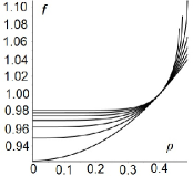
Figure 1: Graphs of $f(\rho)$ for $f(\frac{2}{5})=1$, $f^{\prime}(\frac{2}{5})=\frac{2}{5}$, $n=2$ and $p=2,3,\ldots,8$.

5 Appendix

Proof.

(of Lemma 1). Using $\delta\,{\bf r}_{i}=u_{i}\,{\bf N}+u\,{\bf N}_{i}$, we calculate

$$\langle\delta\,{\bf r}_{i},{\bf r}_{j}\rangle=\langle u_{i}\,{\bf N}+u\,{\bf N}_{i},{\bf r}_{j}\rangle=\,u\,\langle{\bf N}_{i},{\bf r}_{j}\rangle=-u\,\langle{\bf N},{\bf r}_{ij}\rangle=-u\,h_{ij}.$$

Thus, since the symmetry $h_{ij}=h_{ji}$ we get the equality (8): $\delta\,g_{ij}=\langle\delta\,{\bf r}_{i},{\bf r}_{j}\rangle+\langle{\bf r}_{i},\delta\,{\bf r}_{j}\rangle=-2\,u\,h_{ij}$. From $g^{il}g_{lj}=\delta^{i}_{j}$ it follows that $(\delta g^{il})g_{lj}=-g^{il}(\delta g_{lj})=2\,u\,g^{il}h_{lj}$; hence, (9) is true.

We will compute the variation of $h$. Using $\langle{\bf N},{\bf N}_{i}\rangle=0$, we find

$$\langle{\bf N},\ \delta\,{\bf r}_{ij}\rangle=\langle{\bf N},\ (u\,{\bf N})_{ij}\rangle=u_{ij}-u\,\langle{\bf N}_{i},\ {\bf N}_{j}\rangle=u_{ij}-u\,\langle{h}^{l}_{i}\,{\bf r}_{l},\ {h}^{k}_{j}\,{\bf r}_{k}\rangle=u_{ij}-u\,{h}^{l}_{i}\,h_{jl}.$$

Note that $\delta\,{\bf N}=c^{i}{\bf r}_{i}$ for some functions $c^{i}$. Using $\langle{\bf N},{\bf r}_{j}\rangle=0$, we get

$$g_{ij}\,c^{i}=\langle\delta\,{\bf N},\ {\bf r}_{j}\rangle=-\langle{\bf N},\ \delta\,{\bf r}_{j}\rangle=-\langle{\bf N},\ u_{j}\,{\bf N}+u\,{\bf N}_{j}\rangle=-u_{j}.$$

It follows that $c^{i}=-g^{ij}u_{j}$ and $\delta\,{\bf N}=-g^{ij}u_{j}{\bf r}_{i}=-u^{i}{\bf r}_{i}$. Using the Gauss equation for a hypersurface in $\mathbb{R}^{n+1}$, we get at $x$: $\langle\delta\,{\bf N},\ {\bf r}_{ij}\rangle=\langle-u^{i}{\bf r}_{i},\ h_{jl}{\bf N}+\Gamma^{k}_{jl}\,{\bf r}_{k}\rangle=0$. Thus, (10) is true:

$$\delta{h}_{ij}=\delta\langle{\bf r}_{ij},\ {\bf N}\rangle=\langle\delta\,{\bf N},\ {\bf r}_{ij}\rangle+\langle{\bf N},\ \delta\,{\bf r}_{ij}\rangle=u_{ij}-u{h}^{l}_{i}\,h_{jl}.$$

Calculating the variation of the mean curvature, we get (12):

$$\delta\,(nH)=\delta\,(g^{ij}h_{ij})=2\,u{h}^{ij}\,h_{ij}+g^{ij}\big{(}u_{ij}-u{h}^{l}_{i}\,h_{jl}\big{)}$$

$$=u\,h_{ij}\,{h}^{ij}+g^{ij}u_{ij}=\Delta u+u\,\|{h}\|^{2}.$$

The formula $\delta({\rm d}V)=\frac{1}{2}\,(\operatorname{trace}_{g}\delta\,g)\,{\rm d}V$ for variation of ${\rm d}V$ is valid for any variation $\delta g$ of a metric. for example, [13]. Applying (8) to the above gives (13). Next, we calculate the variation of $\|{h}\|^{2}$:

$$\quad\delta\,\|{h}\|^{2}=\delta\,(g^{ik}g^{jl}h_{kl}h_{ij})$$

$$=2\,u\big{(}{h}^{ik}g^{jl}+{h}^{jl}g^{ik}\big{)}h_{kl}h_{ij}+g^{ik}g^{jl}\big{(}(u_{kl}-u{h}^{q}_{k}h_{lq})h_{ij}+(u_{ij}-u{h}^{q}_{i}h_{jq})h_{kl}\big{)}$$

$$=2\,(uh_{ij}{h}^{ik}{h}^{j}_{k}+u_{kl}\,g^{ik}g^{jl})=2\,u\,\langle{h},\ {h}^{2}\rangle+2\,\langle{h},{\rm Hess}_{\,u}\rangle,$$

that proves (11). ∎

Proof.

(of Lemma 3) First, using (8) and (10), we get for $1\leq i,j\leq s$ and $1\leq q\leq n$,

$$\delta\,(s\,{H}_{\cal F})=\delta\,(g^{ij}h_{ij})=2\,u{h}^{ij}\,h_{ij}+g^{ij}\big{(}u_{ij}-u{h}^{q}_{i}\,h_{jq}\big{)}=\Delta_{\,\cal F}\,u+u\,(\|h_{\cal F}\|^{2}-\|h_{\rm mix}\|^{2}),$$

that proves (16). Also for $1\leq i,j,k,l\leq s$ and $1\leq q\leq n$ we obtain (17):

$$\delta\,\|h_{\cal F}\|^{2}=\delta(g^{ik}g^{jl}h_{kl}h_{ij})$$

$$=2\,u\big{(}{h}^{ik}g^{jl}+{h}^{jl}g^{ik}\big{)}h_{kl}h_{ij}+g^{ik}g^{jl}\big{(}(u_{kl}-u{h}^{q}_{k}h_{lq})h_{ij}+(u_{ij}-u{h}^{q}_{i}h_{jq})h_{kl}\big{)}$$

$$=4\,u\,\langle h_{\cal F},h_{\cal F}^{2}\rangle+2\,\langle h_{\cal F},{\rm Hess}^{\,\cal F}_{\,u}\rangle-2\,u\,\langle h_{\cal F},h_{\cal F}^{2}\rangle-2\,u\,\langle h_{\cal F},h_{\rm mix}^{2}\rangle.$$

For $1\leq i,j,k,l\leq s$, $s<\alpha,\beta,\gamma\leq n$ and $1\leq q\leq n$ we obtain (18):

$$\delta\,\|h_{\rm mix}\|^{2}=\delta(g^{ij}g^{\alpha\beta}h_{i\alpha}h_{j\beta})$$

$$=2\,u\big{(}{h}^{ij}g^{\alpha\beta}+{g}^{ij}h^{\alpha\beta}\big{)}h_{i\alpha}h_{j\beta}+g^{ij}g^{\alpha\beta}\big{(}u_{i\alpha}h_{j\beta}+u_{j\beta}h_{i\alpha}\big{)}-u\,g^{ij}g^{\alpha\beta}\big{(}h^{l}_{i}h_{\alpha l}h_{j\beta}+h^{l}_{j}h_{\alpha i}h_{l\beta}\big{)}$$

$$=\langle h_{\cal F}+h_{\cal F^{\perp}},u\,h_{\rm mix}^{2}\rangle+2\,\langle h_{\rm mix},{\rm Hess}^{\,\rm mix}_{\,u}\rangle.$$

The proof of (19) is similar to the proof of [8, Eq. (19)]: instead of $M^{2}$ we consider $s$-dimensional leaves of $\cal F$. The variation of the Christoffel symbols is the following tensor, e.g., [8]:

$$\delta\,\Gamma^{k}_{ij}=-u\,g^{kl}\big{(}h_{jl,i}+h_{il,j}-h_{ij,l}\big{)}-g^{kl}\big{(}u_{i}h_{jl}+u_{j}h_{il}-u_{l}h_{ij}\big{)}.$$ (56)

For the Laplacian $\Delta_{\,\cal F}\,f=g^{ij}\,(f_{ij}-\Gamma^{k}_{ij}\,f_{k})$ with $1\leq i,j,k\leq s$ it follows that

$$\delta\,(\Delta_{\,\cal F}\,f)=\delta\,(g^{ij}f_{ij})-\delta\,(g^{ij}\Gamma^{k}_{ij}f_{k}).$$ (57)

For the first term we get (for $1\leq i,j\leq s$)

$$\delta\,(g^{ij}f_{ij})=2\,u\,h^{ij}f_{ij}+g^{ij}\dot{f}_{ij}=2\,u\,\langle h_{\cal F},\,{\rm Hess}^{\,\cal F}_{f}\rangle+\Delta_{\,\cal F}\,\dot{f}.$$ (58)

For the second term, using (56) and $\Gamma^{k}_{ij}=0$ at $x$, we get for $1\leq i,j,k\leq s$ and $1\leq q\leq n$,

$$\delta\,(g^{ij}\,\Gamma^{k}_{ij}f_{k})=g^{ij}\delta\,(\Gamma^{k}_{ij})f_{k}=-g^{ij}g^{kq}\big{\{}u\,(h_{jq,i}+h_{iq,j}-h_{ij,q})f_{k}-(u_{i}h_{jq}+u_{j}h_{iq}-u_{q}h_{ij})f_{k}\big{\}}$$

$$=-2\,u\,g^{ij}\,g^{kq}h_{jq,i}f_{k}+u\,g^{ij}\,g^{kq}h_{ij,q}f_{k}-2\,g^{ij}\,g^{kq}u_{i}h_{jq}f_{k}+g^{ij}\,g^{kq}\,u_{q}h_{ij}f_{k}.$$ (59)

Using the Codazzi-Minardi equation $\nabla_{k}\,h_{ij}-\nabla_{j}\,h_{ik}=0$, e.g., [11], we get for $1\leq i,j,k,l\leq s$,

$$g^{ij}\,g^{kl}(\nabla_{j}\,h_{il})f_{k}=g^{kl}(g^{ij}\nabla_{l}\,h_{ij})f_{k}=s\,(\nabla^{k}H_{\cal F})f_{k}=s\,\langle\nabla^{\cal F}H_{\cal F},\,\nabla^{\cal F}f\rangle.$$

Thus, using normal coordinates and $-2\,u\,g^{ij}g^{kl}h_{jl,i}\,f_{k}+u\,g^{ij}g^{kl}h_{ij,l}f_{k}=-u\,g^{kl}(g^{ij}h_{ij,l})f_{k}$, we get $s\,(H_{\cal F})_{l}=g^{ij}\,\nabla_{l}\,h_{ij}$ for $1\leq i,j,l\leq s$. Therefore, (5) becomes

$$\delta\,(g^{ij}\,\Gamma^{k}_{ij}f_{k})=-u\,g^{kl}(g^{ij}h_{ij,l})f_{k}-2\,g^{ij}g^{kl}u_{i}h_{jl}f_{k}+g^{kl}u_{l}(g^{ij}h_{ij})f_{k}$$

$$=-s\,u\,\langle\nabla^{\cal F}H_{\cal F},\nabla^{\cal F}f\rangle-2\,h(\nabla^{\cal F}u,\nabla^{\cal F}f)+s\,H_{\cal F}\langle\nabla^{\cal F}u,\nabla^{\cal F}f\rangle.$$ (60)

Applying (58) and (5) to (57) completes the proof of (19). ∎

Proof.

(of Lemma 5) We have $\Delta_{\,\cal F}\,f_{2}={\rm div}_{\cal F}(\nabla^{\,\cal F}f_{2})$. One can show that ${\rm div}_{\cal F}\,(PX)={\rm div}\,(PX)-({\rm div}\,P)(PX)$ for all $X\in\mathfrak{X}_{M}$. Hence, using $\nabla^{\,\cal F}f=P\nabla f$ and (20), we get

$$f_{1}\Delta_{\,\cal F}\,f_{2}=f_{1}\,{\rm div}_{\,\cal F}(\nabla^{\,\cal F}f_{2})=f_{1}\big{\{}{\rm div}(P\nabla f_{2})-({\rm div}\,P)(P\nabla f_{2})\big{\}}$$

$$={\rm div}\,(f_{1}\,P\nabla f_{2})-\langle P\nabla f_{1},P\nabla f_{2}\rangle={\rm div}\,(f_{1}\,P\nabla f_{2})-\langle\nabla^{\,\cal F}f_{1},\nabla^{\,\cal F}f_{2}\rangle.$$

Using the Divergence Theorem, gives

$$\int_{M}f_{1}(\Delta_{\,\cal F}\,f_{2})\,{\rm d}V=-\int_{M}\big{\langle}\nabla^{\,\cal F}f_{1},\nabla^{\,\cal F}f_{2}\big{\rangle}\,{\rm d}V.$$ (61)

By this, the formula (22) is true. Next, using (20) we will prove

$$\int_{M}\langle\varphi_{1},\nabla^{\cal F}\varphi_{2}\rangle\,{\rm d}V=\int_{M}\langle\nabla^{\cal F*}\varphi_{1},\varphi_{2}\rangle\,{\rm d}V$$ (62)

for any compactly supported $(s,t)$-tensor $\varphi_{1}$ and $(s,t+1)$-tensor $\varphi_{2}$. Define a compactly supported 1-form $\omega$ by $\omega(Y)=\langle\iota_{\,Y}\,\varphi_{2},\,\varphi_{1}\rangle$ for $Y\in{\mathcal{X}}_{M}$. Take an orthonormal frame $(e_{i})$ such that $\nabla_{Y}e_{i}=0$ for all $Y\in T_{x}M$ and some $x\in M$. To simplify calculations, assume that $s=t=1$, then at $x\in M$,

$$-\nabla^{*{\cal F}}\omega=\sum\nolimits_{j}(\nabla^{\cal F}_{e_{j}}\,\omega)(e_{j})=\sum\nolimits_{i,j}\langle{P}e_{j},e_{i}\rangle\,(\nabla_{e_{i}}\,\omega)(e_{j})$$

$$=\sum\nolimits_{i,j,c}\langle{P}e_{j},e_{i}\rangle\big{(}\langle\nabla_{e_{i}}\varphi_{2}(e_{j},e_{c}),\varphi_{1}(e_{c})\rangle+\langle\varphi_{2}(e_{j},e_{c}),\nabla_{e_{i}}\varphi_{1}(e_{c})\rangle\big{)}$$

$$=\!\sum\nolimits_{i,j,c}\big{[}\langle\,\langle{P}e_{j},e_{i}\rangle\nabla_{e_{i}}\varphi_{2}(e_{j},e_{c}),\varphi_{1}(e_{c})\rangle{+}\langle\varphi_{2}(e_{j},e_{c}),\langle{P}e_{j},e_{i}\rangle\nabla_{e_{i}}\varphi_{1}(e_{c})\rangle\big{]}$$

$$=\sum\nolimits_{j,c}\big{[}\langle\nabla^{\cal F}_{e_{j}}\varphi_{2}(e_{j},e_{c}),\varphi_{1}(e_{c})\rangle+\langle\varphi_{2}(e_{j},e_{c}),\nabla^{\cal F}_{e_{j}}\varphi_{1}(e_{c})\rangle\big{]}=\langle\varphi_{2},\nabla^{\cal F}\varphi_{1}\rangle-\langle\nabla^{*{\cal F}}\varphi_{2},\varphi_{1}\rangle.$$

The $\nabla^{{\cal F}*}$ is related to the ${\cal F}$-divergence of a vector field $\omega^{\sharp}$ by ${\rm div}_{\cal F}\,\omega^{\sharp}=-\nabla^{{\cal F}*}\,\omega$. By the above and $\int_{M}({\rm div}_{\cal F}\ \omega^{\sharp})\,{\rm d}V=\int_{M}{\rm div}(P\omega^{\sharp})\,{\rm d}V=0$, we obtain (62). Applying this twice, we get (23). ∎

References

- [1] Berger, M. A panoramic view of Riemannian geometry. Springer-Verlag, Heidelberg, 2002.
- [2] Chang, Yu-C. Willmore surfaces and -Willmore surfaces in space forms. Taiwanese J. Math. 17, No. 1, 109–131 (2013).
- [3] Chen, B.-Y. On a theorem of Fenchel-Borsuk-Willmore-Chern-Lashof. Mathematische Annalen, 194(1) 1971, 19–26.
- [4] Chen, B. Y. On the total curvature of immersed manifolds. II. Mean curvature and length of second fundamental form. Amer. J. Math., 94, 799–809 (1972)
- [5] A. Candel and L. Conlon, Foliations, I and II, Grad. Studies in Math. 60, AMS, 2000, 2003.
- [6] Guo, Z. Generalized Willmore functionals and related variational problems. Diff. Geom. Appl., 25 (2007), 543–551
- [7] Guo, Z. Higher order Willmore hypersurfaces in Euclidean space. Acta Math. Sin., Engl. Ser. 25, No. 1 (2009), 77–84
- [8] Gruber, A., Toda, M., Tran H. On the variation of curvature functionals in a space form with application to a generalized Willmore energy. Annals of Global Analysis and Geometry (2019) 56 : 147–165
- [9] Li, J., Guo, Z. Higher order Willmore revolution hypersurfaes in . Lifelong Education, Vol. 10, Issue 3 (2021) 75–89
- [10] Marques, F. C., Neves, A. Min-max theory and the Willmore conjecture. Ann. Math. 179, No. 2 (2014), 683–782.
- [11] Petersen, P. Riemannian geometry, 3 rd ed. Springer, 2016.
- [12] Reilly, R.C. Variational properties of functions of the mean curvatures for hypersurfaces in space forms. J. Differ. Geom. 8, 465–477 (1973).
- [13] Rovenski, V., Walczak, P. Extrinsic geometry of foliations, Birkhäuser, Progress in Mathematics, Vol. 339, 2021.
- [14] Song, A. Generation of tubular and membranous shape textures with curvature functionals. Journal of Mathematical Imaging and Vision (2022) 64 : 17–40
- [15] Willmore, T.J. Note on embedded surfaces. An. Stiint. Univ. “AI. I. Cuza” Iasi, Sect. Ia Mat. 11. (1965), 493–496.
- [16] Zhu, Y., Liu, J., Wu, G.. Gap phenomenon of an abstract Willmore type functional of hypersurface in unit sphere. Scientific World J., Vol. 2014, Article ID 697132, 8 pages.