PHNet: Patch-based Normalization for Portrait Harmonization

Abstract

A common problem for composite images is the incompatibility of their foreground and background components. Image harmonization aims to solve this problem, making the whole image look more authentic and coherent. Most existing solutions predict lookup tables (LUTs) or reconstruct images, utilizing various attributes of composite images. Recent approaches have primarily focused on employing global transformations like normalization and color curve rendering to achieve visual consistency, and they often overlook the importance of local visual coherence. We present a patch-based harmonization network consisting of novel Patch-based normalization (PN) blocks and a feature extractor based on statistical color transfer. Extensive experiments demonstrate the network’s high generalization capability for different domains. Our network achieves state-of-the-art results on the iHarmony4 dataset. Also, we created a new human portrait harmonization dataset based on FFHQ and checked the proposed method to show the generalization ability by achieving the best metrics on it. The benchmark experiments confirm that the suggested patch-based normalization block and feature extractor effectively improve the network’s capability to harmonize portraits. Our code and model baselines are publicly available.

1 Introduction

Image composition, a prevalent task in computer vision, involves merging elements from different sources to create unique visuals. The outcome can be distinct and exceptional when merging images from various origins. However, incorporating the object into a new background frequently leads to unrealistic appearances. Creating a realistic composite image often involves manually adapting the foreground object’s appearance to harmonize with the background. This process entails meticulous adjustments, demanding human expertise and specialized photo editing tools. Image harmonization aims to make the composited image visually consistent and indistinguishable, alleviating the constraints of manual editing. On the other hand, the problem is ill-posed due to the ambiguity of human eye perception. As a result, visual comparison of the composites only sometimes matches with quantitative results.

Traditional color space transformation methods have long been used to harmonize foreground objects with new backgrounds. These approaches typically involve independently computing statistics for the foreground object and the new background. The fundamental concept is to align the color distribution of the object with that of the background, shifting the object’s color characteristics to match the background better. However, it is essential to note that these conventional techniques lack consideration of semantic information. Their primary reliance is on color-based transformations, and although practical to some extent, these frequently give rise to unwanted artifacts and visually displeasing outcomes. Recent works try to solve the harmonization problem with encoder-decoder networks[8, 16, 7] and transformers[9], trying to enrich low-level representations with auxiliary features.

Nevertheless, most prior research in this domain has predominantly approached the broader issue of harmonization without concentrating on a particular and highly practical subtask, namely portrait harmonization. The growing significance of this subtask can be attributed to the widespread use of video conferencing and various social media applications in our daily routines, making it arguably the most common and impactful usage of image harmonization [27].

This work aims to explore solutions for producing visual-pleasant image composites. We propose a Patch-based Harmonization Network (PHNet) with our novel patch-based normalization block (PN) and feature extraction (PFE) module to obtain realistic results. We emphasize enhancing portrait harmonization, as recent approaches overlook this domain adaptation problem. Since no open portrait harmonization datasets are available and the public dataset iHarmony4 consists of a small number of portrait images, we collect a new portrait harmonization dataset based on Flickr-Faces-HQ [13] and provide extensive experiments on portraits.

Our contributions can be summarized as follows:

• The innovative image harmonization method showcased in this study has proven remarkably effective, consistently achieving concurrent metrics on publicly available datasets.

• We introduce a synthetic portrait dataset explicitly designed for the harmonization task, enriching the resources available for research in this domain. We also make the demo application code and baselines available as open-source.

• We conduct a comprehensive set of experiments to evaluate the performance of our approach, comparing it against existing methodologies. The extensive experiments provide compelling evidence of the superiority of our method, both in terms of quantitative metrics and qualitative visual results. Notably, our approach stands out by achieving state-of-the-art performance on the collected portrait harmonization dataset, reaffirming its prowess in the portrait harmonization task.

2 Related Work

The harmonization problem can be formulated as follows: suppose we have an image composited of foreground object F with mask M and background B. The objective is to optimize the harmonization function H to ensure the harmonized image I aligns seamlessly with the background, giving the impression that the image was not a composition of two distinct pictures:

$$I=H(F,B)\cdot M+(1-M)\cdot B$$ (1)

Traditional image harmonization methods mainly process images by changing low-level features in color space using color distribution transfer[21, 19, 20], multi-scale color statistics[24] or gradient-based methods[18, 26].

In recent years, neural networks have shown significant advances in image harmonization tasks. DoveNet[8] treats image harmonization as a domain translation task and uses information from the background to guide the foreground harmonization. In RainNet[16], the Region-aware Adaptive Instance Normalization (RAIN) module was introduced, which can capture background statistical features and use them to normalize foreground features. CDTNet[7] employed pixel-to-pixel transformations obtained by an encoder-decoder network and RGB-to-RBG transformations performed by several 3D LUTs. Some methods, such as Harmonizer[14] and DCCF[28], aim to directly learn different color transformation filters (for example, hue and saturation) in order to perform white-box harmonization. In IntrinsicHarmony[10], authors presented a new perspective on image harmonization, later continued in [9], where the first harmonization transformer was introduced. They decomposed the scene into two intrinsic characteristics: material-dependent reflectance and light-dependent illumination, which can be harmonized separately. In HDNet[2], authors proposed an encoder-decoder architecture with local and global dynamic modules for feature map refinement. In [15], a pre-trained classification network extracts high-level semantic representations to feed them into a decoder. Authors of DucoNet[25] inspired by StyleGAN2[13] and extracted control codes from the separate channels in the Lab color space to generate dynamic convolution kernels used in the decoder as weights for StyleBlock. GKNet[22] employs multi-head attention before predicting adaptive kernels for application at various decoder network stages. LRIP[3] divided the image into different numbers of patches into different stages of the decoder and applied a stack of MLPs to them, with the weights predicted from the encoder features.

However, none of these methods are explicitly trained for the portrait harmonization task and, therefore, need better performance when used in this domain. In [27], authors focus on the portrait harmonization problem but solve it interactively: the model needs guidance from the user to harmonize the composite. In this paper, we aim to address the challenge of image harmonization and develop a network that can excel in both general image harmonization and portrait-specific scenarios.

3 Datasets

3.1 Harmonization Datasets

Numerous datasets exist for image harmonization, although most offer a limited number of samples and need to be revised for the specific requirements of portrait harmonization. GMSDataset[23] and RealHM[12] datasets contain 183 and 216 images, respectively, which is insufficient for model training. HVIDIT[10] and RdHarmony[1] consist of rendered scenes and may not apply to authentic image harmonization.

Solely serving as the harmonization benchmark, iHarmony4[8] stands as the only large-scale harmonization dataset publicly accessible. Comprising four subsets - HCOCO, HAdobe5k, Hday2night, and HFlickr - the dataset includes 73,146 pairs encompassing composite images, corresponding ground-truth images, and associated foreground masks.

All datasets mentioned above are unsuitable for the portrait harmonization task: images in these datasets usually portray inanimate objects, animals, nature, or full-body scenes, but not portraits. There is one open portrait harmonization test dataset, PortraitTest[27], but it is not compatible with our model since authors harmonize images interactively. The authors suggest harmonizing the target human in the composite image by utilizing the knowledge of the already harmonized human in the background, which limits our approach as we focus on solving the problem of harmonizing a single human. These reasons prompted us to create a new dataset specifically for portrait harmonization.

3.2 Our Dataset

3.2.1 Dataset creation.

In this work, we present Flickr-Faces-HQ-Harmonization (FFHQH), a new dataset for portrait harmonization based on the FFHQ [13]. It contains real images, foreground masks, and synthesized composites. Generating composite images has two steps: alpha mask generation and color augmentation. For mask generation, we employed the portrait matting network StyleMatte[5]. Then, we obtained foreground objects and applied color augmentations, such as brightness, contrast, hue, and sharpness adjustment. Lastly, we blended the augmented object with an unchanged background. We carefully chose the range of augmentation parameters to avoid extreme color distortion and keep the image appearance realistic. The applied augmentations include ColorJitter, with parameters for adjusting brightness (0.5), contrast (0.4), saturation (0.06), and hue (0.05). RandomPosterize is employed with a probability of 0.5, introducing posterization with a range of 6. RandomAdjustSharpness is incorporated with a range of 4 and a probability of 0.5 to randomly adjust sharpness. Furthermore, RandomAutocontrast is applied with a probability of 0.5 to introduce random autocontrast transformations. These augmentations collectively contribute to the diversification of the dataset, enhancing its robustness and generalization capabilities for subsequent scientific analyses. We provide visual examples in the supplementary materials.

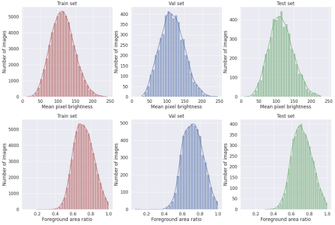
Figure 1: FFHQH dataset statistics. Histograms illustrate the distribution of image brightness and foreground area ratio.

3.2.2 Dataset description.

FFHQH dataset consists of 70,000 images of human faces at $1024\times 1024$ resolution and has all the advantages of the original FFHQ dataset regarding variation in poses, identities, backgrounds, and attributes (hair, freckles). We randomly split the data into training, validation, and test sets with 60,000, 5,000, and 5,000 samples. The distributions of pixel brightness and foreground area ratio in FFHQH are shown on Fig. 1. It can be noted that pixel brightness follows a normal distribution centered around a mean value of approximately 113. On average, the foreground occupies 70% of the entire image, suggesting that our dataset predominantly contains large foreground objects. The mean and standard deviation values for RGB channels separately are [0.51, 0.42, 0.37] and [0.25, 0.23, 0.23], respectively.

4 Architecture

In this section, we present our approach to image harmonization. Firstly, we define the normalization block, which utilizes color transfer statistical methods. Further, we describe the feature extraction module that helps acquire high-level background representation. Lastly, we give an overview of our end-to-end architecture.

4.1 Patch-based normalization

Patch-based normalization (PN) block aims to normalize images based on global and local statistics. Consider the foreground image as $\mathit{F\in\bbbr^{C\times H\times W}}$, the background image as $\mathit{B\in\bbbr^{C\times H\times W}}$ and the object mask as $\mathit{M\in\bbbr^{H\times W}}$. Let us denote the number of pixels as $N$ and the number of patches into which we divide the input as $P$. Initially, we compute both the standard mean and deviation for the entire image and each patch individually by:

$$\mu_{glob}(I)=\frac{\sum\limits_{x\in I}{x}}{N},\>\mu_{loc}^{i}(I)=\frac{\sum\limits_{x\in p(I,i)}{x}}{N_{i}}$$ (2)

$$\sigma_{glob}(I)=\sqrt{\frac{\sum\limits_{x\in I}{(x-\mu_{glob}(I))^{2}}}{N}}$$ (3)

$$\sigma_{loc}^{i}(I)=\sqrt{\frac{\sum\limits_{x\in p(I,i)}{(x-\mu_{loc}^{i}(I))^{2}}}{N_{i}}}$$ (4)

The $p(I,i)$ denotes the i-th patch of the input $I$ when we split it into a grid, as shown in Fig. 2. The number of splits along both axes is equal and varies in the range $[1,\sqrt{N}]$.

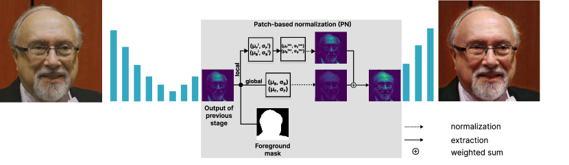
Figure 2: Patch-based Normalization (PN) block. Only one stage of the decoder is demonstrated for visual simplicity. The corresponding foreground mask is resized and fed to the block along with the previous stage output. Local and global branches compute a set of statistics and modify feature maps independently, as described in Sec. 4. Afterward, these results are combined and fed into the next decoding layer.

We compute statistics in a per-channel manner for background and foreground. Given only a composite image and harmonization mask, we extract $F$ and $B$ by multiplying the mask with the composite. Next, we apply local and global normalization separately.

For global normalization, we use computed global mean and deviation coefficients. At this stage, the background remains unchanged. We update only the foreground object, transferring its color space based on the background characteristics. To do so, we firstly shift the object distribution to standard normal using $\mu_{glob}(F)$ and $\sigma_{glob}(F)$, then apply $\mu_{glob}(B)$ and $\sigma_{glob}(B)$ to get closer to the background’s color distribution:

$$\mathit{\hat{F}}_{glob}=[\mathit{F}-\mu_{glob}(F)]\frac{\sigma_{glob}(B)}{\sigma_{glob}(F)}+\mu_{glob}(B)$$ (5)

For local normalization, we first compute patch-based scale and shift coefficients summing up computed local statistics:

$$\mu_{loc}(I)=\sum_{i=1}^{P}\alpha^{i}(I)\cdot\mu_{loc}^{i}(I),$$ (6)

$$\sigma_{loc}(I)=\sqrt{\frac{\sum\limits_{i=1}^{P}\beta^{i}(I)\cdot\sigma_{loc}^{i}(I)^{2}}{P}}$$ (7)

where $\alpha^{i}$, $\beta^{i}$ are the learned scores for each patch. We assume that different patches are primarily independent, and their distributions differ, so we utilize the scaled sum of variances to compute the local scale coefficient.

Afterward, we normalize background and foreground images in the same manner as we computed $\hat{F}_{glob}$ in Eq. 5, utilizing local statistics ahead of the global ones:

$$\mathit{\hat{F}}_{loc}=[\mathit{F}-\mu_{glob}(F)]\frac{\sigma_{loc}(B)}{\sigma_{glob}(F)}+\mu_{loc}(B)$$ (8)

$$\mathit{\hat{B}}_{loc}=[\mathit{B}-\mu_{glob}(B)]\frac{\sigma_{loc}(B)}{\sigma_{glob}(B)}+\mu_{loc}(B)$$ (9)

Lastly, our PN-block computes a weighted sum of locally and globally normalized images and blends them with the original background:

$$\mathit{\tilde{F}}=w_{0}\cdot\mathit{\hat{F}}_{loc}+w_{1}\cdot\mathit{\hat{F}}_{glob}+w_{2}$$ (10)

$$\mathit{\tilde{B}}=\gamma_{0}\cdot\mathit{\hat{B}}_{loc}+\gamma_{1}\cdot B+\gamma_{2}$$ (11)

where $\gamma_{0},\gamma_{1},\gamma_{2}$ and $w_{0},w_{1},w_{2}$ are trainable linear parameters. Finally, the normalized image is extracted using blending of Eq. 10 and Eq. 11 with the given mask:

$$N(F,B,M)=\tilde{F}\cdot M+\tilde{B}\cdot(1-M)$$ (12)

4.2 Patch-based feature extraction

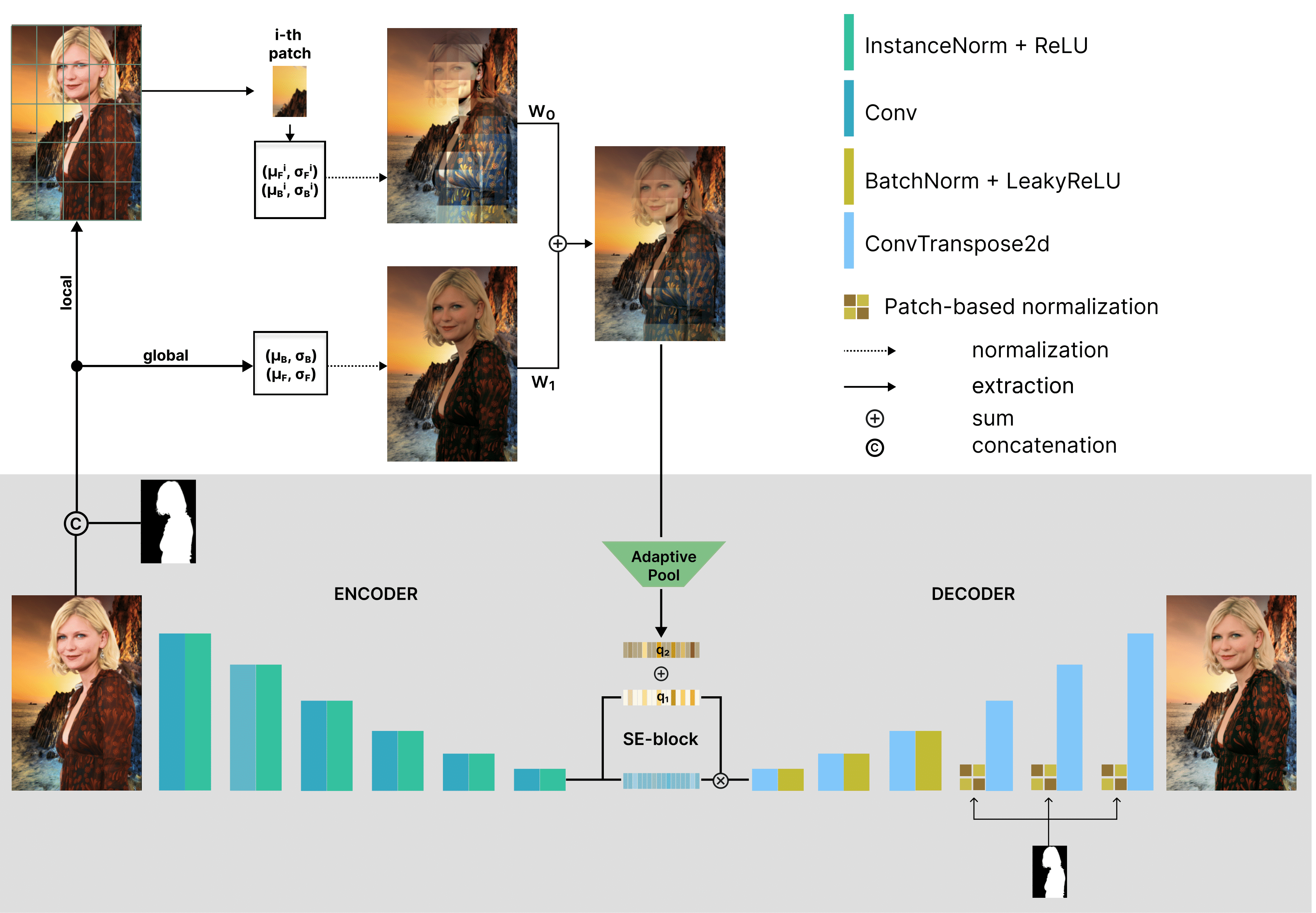
Figure 3: Overview of the PHNet architecture. The gray block highlights the autoencoder, while in the upper left, we showcase the pipeline of our patch-based feature extractor (PFE). The modified squeeze and excitation block is denoted as SE. To enhance clarity, skip connections between the Decoder and Encoder are omitted. Within the Decoder, we illustrate the resized foreground masks fed into Patch-based normalization blocks. An Adaptive Pooling layer extracts the auxiliary vector $q_{2}$ from the PFE block output, which is then forwarded to the SE block.

We use the idea of patch-based normalization to construct a feature extraction module (PFE). As shown in Fig. 3, the PFE module is similar to PN-block with only trainable parameters $w_{0}$ and $w_{1}$ from Eq. 10. All of the other parameters are fixed and do not require training. The PFE module outcomes are then adaptively averaged and used as auxiliary coefficients to reweight channels after squeezing them in the last layer of our encoder (Fig. 3). The intuition of such a block comes from experiments with composite images, wherein it is possible to manipulate the foreground to blend into the background to the point that it almost vanishes, all while retaining color-independent attributes, as shown in Fig. 3.

4.3 Network architecture

We utilize encoder-decoder architecture featuring a Squeeze-and-Excitation[11] block. This strategy enables the model to remain unaffected by variations in image resolution. Furthermore, it incorporates an attention mechanism that helps obtain intuitive weights for feature map channels. We integrated this mechanism into our patch-based feature extraction module, utilizing a patch count of 25, and summed the PFE module’s result vector with the SE-block weights. Our main contribution is the patch-based normalization (PN) block, which helps to normalize images based on statistics collected on background patches. We use PN-blocks in the last 3 layers of the decoder with the count of patches equal to 9, 16, and 25, respectively. The lower layers of the decoder apply batch normalization for network regularization. We utilize transposed convolutions to upsample feature maps followed by PN-blocks and LeakyReLU activation. In the encoder part, we propose convolutions followed by instance normalization and ReLU activation. Finally, to maintain the original background, we blended it with the network output. The complete architecture is shown in Fig. 3.

4.4 Objective function

We employed the weighted sum of several losses in the training process to achieve realistic results and alleviate visual artifacts. We impose new $\mathcal{L}_{PSNR}$ to directly optimize the Peak Signal-to-Noise Ratio, one of our key metrics. Considering $\hat{I}$ is the predicted image, $I$ is the corresponding ground-truth image, and $I_{max}$ is the maximum value of the target image, PSNR-Loss is denoted by:

$$\mathcal{L}_{PSNR}{(\hat{I})}=\frac{100}{\log_{10}\frac{{max(I)}}{\|{\hat{I}}-{I}\|_{2}}}$$ (13)

Also, even though the variation in mask size in FFHQH is not significant, we use Foreground-Normalized MSE (FN-MSE)[15], which ensures the same penalty magnitude for images with masks of different scales:

$$\mathcal{L}_{FN-MSE}{(\hat{I})}=\frac{\|{\hat{I}}-{I}\|_{2}^{2}}{\max\left\{A_{min},\sum\limits_{x\in M}{x}\right\}},$$ (14)

where $M$ denotes the foreground binary mask. We assign $A_{min}$ equal to 100 as in the original paper.

To alleviate blurring artifacts of the autoencoder, we also utilize $\mathcal{L}_{G}$ that computes the MSE of gradients. Therefore, our overall objective for training is the weighted sum of the functions mentioned above. We carefully choose their weights to achieve numerical stability and faster convergence:

$$\mathcal{L}=\lambda_{0}\times\mathcal{L}_{PSNR}+\lambda_{1}\times\mathcal{L}_{FN-MSE}+\lambda_{2}\times\mathcal{L}_{G},$$ (15)

where $\lambda_{1}=\lambda_{2}=0.01$, $\lambda_{0}=0.2$.

5 Experiments

5.1 Training details

We conducted an end-to-end training of our network through a series of sequential stages. Firstly, the PFE module was not involved in the SE-block, and only the encoder-decoder part of the network is trained with a learning rate set to 1e-4 for 100 epochs. Subsequently, once network upsampling layers could generate visually satisfactory results, we added the patch-based feature extraction block, froze the encoder, and tuned the network with a learning rate up to 1e-5 for 10 epochs. Finally, we trained an entire network with a lower learning rate (1e-7) for 50 epochs. The whole training process is done on iHarmony4 training set on $256\times 256$ resolution. We run the training process on NVIDIA Tesla V100 with a batch size of 16. We utilized the Lion[4] optimizer to speed up training convergence.

As for FFHQH experiments, we utilized a similar training process with the same objective function. We resized images and collected experiments on $256\times 256$, $512\times 512$, and $1024\times 1024$ resolutions separately.

Table 1: Different setups of our model. $D_{i}$ denotes which layers of Decoder use PN-blocks and PFE denotes the Patch-based Feature Extraction module.

Setup	PSNR $\uparrow$	MSE $\downarrow$
$D_{6}$	32.23	45.03
$D_{6}$ + PFE	34.31	42.23
$D_{5,6}$	35.52	38.16
$D_{5,6}$ + PFE	35.58	37.01
$D_{4,5,6}$	36.55	37.22
$D_{4,5,6}$ + PFE	38.54	16.05
$D_{3,4,5,6}$	36.33	31.69
$D_{3,4,5,6}$ + PFE	37.44	29.68

Table 2: Ablation study. We trained our model on iHarmony4 and FFHQH training sets separately and measured metrics on corresponding test sets. The image resolution is fixed for training and validation.

Resolution	iHarmony4		FFHQH
	PSNR $\uparrow$	MSE $\downarrow$	PSNR $\uparrow$	MSE
$256\times 256$	37.41	24.22	35.84	18.24
$512\times 512$	38.54	16.05	36.44	16.27
$1024\times 1024$	38.24	20.14	35.14	23.15

5.2 Ablation study

5.2.1 Setups.

We employed various network configurations in our experiments. While the suggested architecture performed effectively, we explored alternative hyperparameters for the normalization and feature extraction modules. Additionally, we conducted comparisons of different optimization algorithms.

We trained the network on $512\times 512$ and $1024\times 1024$ resolutions. The training strategy was similar to our primary strategy. In Tab. 2, we demonstrate the results. While our method excels in producing better results at intermediate resolutions, we achieved enhanced high-resolution results by training the network on the FFHQH synthetic dataset with HD resolution. It proves that the portrait harmonization domain is considerably different. The visual study also indicates that a model trained on a synthetic dataset yields more appealing and precise portrait composites. Another noteworthy aspect to highlight is the substantial influence of the Lion optimizer. It speeds up the model convergence by about $10\%$ and regularizes the training process, making it much more stable than the AdamW optimizer[17].

Our best setup model ($D_{4,5,6}$ with PFE in Tab. 1) has $39.9$ million parameters, consuming $153$MB of disk space. We also measured the performance speed on CPU and GPU memory units. On a single Intel H470 CPU thread, PHNet achieves $1.01$ FPS and $34.49$ on a single NVIDIA Tesla V100.

5.2.2 PFE and PN-blocks.

The extracted features and patch-based normalization blocks significantly impact the network’s performance. In Tab. 1, we show that our model results in worse MSE and PSNR metrics without the PFE module. Also, we carefully choose hyperparameters of PN blocks and their location in the decoder. The efficiency of normalization blocks reduces when they are utilized in more than 4 layers of the decoder. We do not insert the normalization blocks in the lower blocks because the produced patches are not large enough for the proposed method and lead to worse convergence.

Our feature extraction module enhances the comprehensibility and induces the intuitiveness of the model. The feature vector obtained from the PFE module illustrates the impact of feature maps on the reconstructed image. This vector encompasses an attention mechanism that assigns probabilities to each encoder output, rendering the feature maps meaningful, akin to heatmaps.

Table 3: Evaluation on FFHQH dataset. All models are trained on the $256\times 256$ resolution.

Model	PSNR $\uparrow$	MSE $\downarrow$	fPSNR $\uparrow$	fMSE $\downarrow$
BargainNet[6]	22.25	715.53	21.25	904.88
DCCF[28]	34.51	34.29	33.07	47.42
D-HT[9]	33.97	39.81	29.19	121.49
RainNet[16]	30.98	84.84	29.52	117.12
IDIH[15]	32.85	47.98	31.39	66.61
iS2AM[15]	33.64	39.85	32.18	55.14
IntrinsicHarmony[10]	31.11	73.22	26.31	224.73
CDTNet[7]	34.25	34.76	32.81	48.1
Harmonizer[14]	27.43	154.86	25.96	215.43
HDNet[2]	32.88	56.4	31.42	76.04
DucoNet[25]	34.82	31.64	33.38	43.81
LRIP[3]	33.73	40.14	32.26	55.6
Ours	35.84	18.24	24.44	34.52

Table 4: Quantitative results on iHarmony4 test dataset.

Model	All		HCOCO		HAdobe5k		Hday2night		HFlickr
Metric	PSNR $\uparrow$	MSE $\downarrow$	PSNR $\uparrow$	MSE $\downarrow$	PSNR $\uparrow$	MSE $\downarrow$	PSNR $\uparrow$	MSE $\downarrow$	PSNR $\uparrow$	MSE $\downarrow$
DoveNet[8]	34.75	52.36	35.83	36.72	34.34	52.32	35.18	54.05	30.21	133.14
BargainNet[6]	35.88	37.82	37.03	24.84	35.34	39.94	35.67	50.98	31.34	97.32
IntrinsicHarmony[10]	35.90	38.71	37.16	24.92	35.20	43.02	35.96	55.53	31.34	105.13
RainNet[16]	36.12	40.29	37.08	-	36.22	-	34.83	-	31.64	-
D-HT[9]	37.55	30.30	38.76	16.79	36.88	38.53	37.10	53.01	33.13	74.51
iS2AM[15]	38.19	24.44	39.16	16.48	38.08	21.88	37.72	40.59	33.56	69.67
CDTNet[7]	38.3	24.04	39.25	16.17	38.26	21.11	37.75	40.74	33.61	69.72
iDIH[15]	38.31	22.00	39.64	14.01	37.35	21.36	37.68	50.61	34.03	60.41
HDNet[2]	37.16	31.32	38.72	18.48	35.87	33.79	36.75	49.14	32.54	88.4
LRIP[3]	37.81	27.56	39.11	16.54	36.91	32.1	38.48	43.25	33.32	70.2
DucoNet[25]	39.17	18.47	40.23	12.12	38.87	17.06	38.11	38.7	34.65	51.71
GKNet[22]	39.53	19.9	40.32	12.95	39.97	17.84	38.47	42.76	34.45	57.58
Ours	38.54	16.05	38.70	14.22	39.98	10.62	40.02	12.70	37.58	34.66

Table 5: Foreground ratio range based results on iHarmony4 test set. The fMSE denotes the foreground region mean squared error.

Model	$0\%\sim 5\%$		$5\%\sim 15\%$		$15\%\sim 100\%$
Metric	MSE $\downarrow$	fMSE $\downarrow$	MSE $\downarrow$	fMSE $\downarrow$	MSE $\downarrow$	fMSE $\downarrow$
DoveNet[8]	14.03	591.88	44.90	504.42	152.07	505.82
BargainNet[6]	10.55	450.33	32.13	359.49	109.23	353.84
IntrinsicHarmony[10]	9.97	441.02	31.51	363.61	110.22	354.84
RainNet[16]	11.66	550.38	32.05	378.69	117.41	389.80
D-HT[9]	9.08	405.32	33.90	385.13	205.40	501.63
iS2AM[15]	6.35	288.19	19.69	226.00	71.68	235.30
CDTNet[7]	6.59	292.28	19.59	223.57	70.81	231.63
iDIH[15]	6.79	296.18	19.43	222.49	61.85	202.80
HDNet[2]	8.58	379.46	25.21	293.15	92.56	298.90
LRIP[3]	7.35	338.81	23.52	267.47	80.33	270.00
DucoNet[25]	5.54	246.40	15.68	179.18	52.49	172.57
GKNet[22]	5.36	244.06	17.46	200.34	57.31	188.75
Ours	6.16	165.89	16.31	158.80	39.72	151.74

6 Evaluation results

In this section, we describe the results of our experiments, evaluate our model on iHarmony4 and FFHQH, and compare it with other state-of-the-art solutions quantitatively and qualitatively.

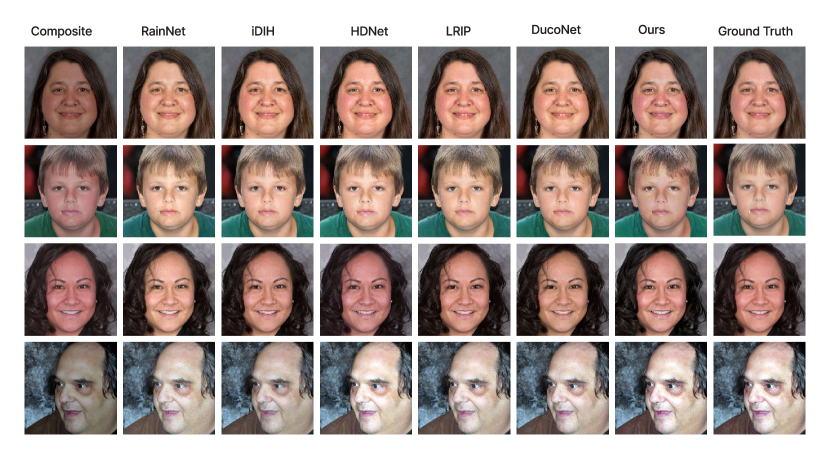
Figure 4: Qualitative comparison on FFHQH. We present the results of four state-of-the-art methods and a proposed model on portrait composites. The samples were taken from our FFHQH dataset.

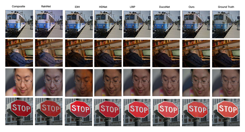
Figure 5: Qualitative comparison on iHarmony4. We present sample results produced by our PHNet compared to four state-of-the-art models. The samples have been sourced from the testing set of iHarmony4[8].

6.0.1 Quantitative comparisons.

We validate our model on a novel FFHQH dataset to compare with other methods. We validate our model on a novel FFHQH dataset to compare with other methods. We evaluate the model by measuring the composite images’ mean squared error (MSE), foreground mean squared error (fMSE), peak signal-to-noise ratio (PSNR) and foreground peak signal-to-noise ratio (fPSNR) (Tab. 3). It can be noted that all models, as expected, perform relatively poorly on previously unseen datasets, which supports our point that models need to be specifically trained for the portrait harmonization task. Nevertheless, even without being trained on FFHQH, the proposed model demonstrates notably favorable results.

Furthermore, we evaluate the performance of our model using iHarmony4 test images. For this purpose, we initially trained the model on the iHarmony4 training dataset and then fine-tuned it on FFHQH, allowing the model to leverage data from different domains. Tab. 4 shows the quantitative results of previous state-of-the-art methods and our model on four subsets. Our method achieves state-of-the-art on subsets HAdobe5k, Hday2night and HFlickr. Our model slightly fails on HCOCO due to a need for a high foreground ratio in the samples. Additionally, we calculate foreground images area ratio $f_{area}$ in composite images in the iHarmony4 test set. It consists of 3830 pictures with $f_{area}<5\%$, 1955 composites with $5\%\leq f_{area}<15\%$ and only 1619 with $f_{area}$ higher than $15\%$, which implies that more samples with larger foreground objects are required. On the contrary, FFHQH dataset contains only samples with $f_{area}>40\%$. For a fair comparison, we computed the mean squared error of the foreground region (fMSE) alongside the whole composite MSE. As mentioned above, we divided the test set into 3 groups and calculated scores for each group separately. Tab. 5 shows that our model achieves the best metrics. The more extensive observation from such an experiment is that all methods perform worse on more prominent foreground objects. Consequently, their ability to harmonize portraits needs further improvement, which is another motivation for collecting our novel portrait harmonization dataset with larger foreground objects. Tab. 3 shows that such domain shift increases model performance in metrics. The visual evidence of this fact is also demonstrated in Fig. 4. It is also worth mentioning that we found some incompatibility in different models due to mask representation ambiguity. We set up our experiments on binary masks because foreground-based metrics differ in the case of matting masks and segmentation masks. Detailed calculations are provided in the appendix.

6.0.2 Qualitative comparisons.

Since the visual appearance of harmonized images does not always correlate with quantitative results, we also conducted a qualitative visual evaluation. We compare our model with six previous harmonization networks: RainNet, HDNet, LRIP, DucoNet, and iDIH. In Fig. 5, we demonstrate that the proposed model reduces the foreground overexposure compared to the ground-truth image, leading to more realistic results. Our method produces images with enhanced visual coherence, ensuring that foreground objects are adjusted to the background in both color temperature and tone.

6.0.3 Limitations.

Our method outperforms related works on the collected FFHQH portrait harmonization dataset. Nevertheless, it has limitations. It may fail to handle non-portrait images due to domain shift and low foreground ratio. As a future work, we would like to tune a more complex harmonization network to address the human-containing composite image harmonization problem. Failure cases are provided in the appendix.

7 Conclusion

We propose a new method for image harmonization. Our novel patch-based normalization block and feature extraction module greatly impacted the retrieved PSNR and MSE metrics. In addition, we study existing harmonization datasets and their relevance to portrait harmonization. We train our network on synthetically collected the FFHQH dataset and demonstrate better qualitative and quantitative results in the portraits domain. Our experiments unequivocally establish the superior performance of the proposed approach over current state-of-the-art methods. These results underscore the need for further investigation into the remaining challenges and areas for improvement. The source code, synthetic dataset FFHQH, and model baselines are publicly available.

Supplementary materials

Appendix 0.A Metrics calculation and masks discrepancies

Remark 1

In the latter works, the authors used non-binary masks obtained by bilinear interpolation for training and metric calculation. Note that only HCOCO in iHarmony4 has non-binary masks, while in the others, they are binary.

Remark 2

We discovered variations in metric computation. Different choices exist for determining the MAX value in the PSNR formula, including the fixed value 255, the maximum value of the target image, and the maximum value minus the minimum value of the input image. We observe this in the related work repositories.

Remark 3

Recent works([7], [25], [15]) use the following fMSE calculation formula:

$$fMSE(\hat{I},I,M)=\frac{\sum\limits_{i=1}^{3}{\sum\limits_{j=1}^{h}{\sum\limits_{k=1}^{w}{M_{j,k}\cdot(\hat{I}_{j,k,i}-I_{j,k,i})^{2}}}}}{3\cdot\sum\limits_{j=1}^{h}{\sum\limits_{k=1}^{w}{M_{j,k}}}},$$ (16)

where $i$ iterates through the 3 RGB channels, $j$ and $k$ - through image height and width.

In the original iHarmony4 repository, fMSE is calculated as follows:

$$\begin{split}fMSE(\hat{I},I,M)=\frac{MSE(\hat{I}\times M,I\times M)\cdot h\cdot w}{\sum\limits_{x\in M}{x}}=\\ =\frac{h\cdot w\cdot\frac{\sum\limits_{i=1}^{3}{\sum\limits_{j=1}^{h}{\sum\limits_{k=1}^{w}{(\hat{I}_{j,k,i}\cdot M_{j,k}-I_{j,k,i}\cdot M_{j,k})^{2}}}}}{3\cdot h\cdot w}}{\sum\limits_{j=1}^{h}{\sum\limits_{k=1}^{w}{M_{j,k}}}}=\\ =\frac{\sum\limits_{i=1}^{3}{\sum\limits_{j=1}^{h}{\sum\limits_{k=1}^{w}{(\hat{I}_{j,k,i}\cdot M_{j,k}-I_{j,k,i}\cdot M_{j,k})^{2}}}}}{3\cdot\sum\limits_{j=1}^{h}{\sum\limits_{k=1}^{w}{M_{j,k}}}}=\\ =\frac{\sum\limits_{i=1}^{3}{\sum\limits_{j=1}^{h}{\sum\limits_{k=1}^{w}{M_{j,k}^{2}\cdot(\hat{I}_{j,k,i}-I_{j,k,i})^{2}}}}}{3\cdot\sum\limits_{j=1}^{h}{\sum\limits_{k=1}^{w}{M_{j,k}}}}\end{split}$$ (17)

The distinction lies in the squared pixels of the mask, and if the masks are not binary, the formulas above will give different results. Nevertheless, recent studies note that after augmentations of iHarmony4 samples, their masks retain a non-binary nature. To ensure fair metric calculation and training across all our experimental setups, we binarized all input masks with threshold 0.5 and utilized them instead of matting masks.

Appendix 0.B Limitations

Figure 6: Failure cases. PHNet can not manage small images with foreground ratio area. In the bottom, we also see bigger foregrounds, but the left example lacks foreground statistics due to being black, while the right one seems to be harmonized not well due to domain shift and still small masked object.

Appendix 0.C FFHQH examples

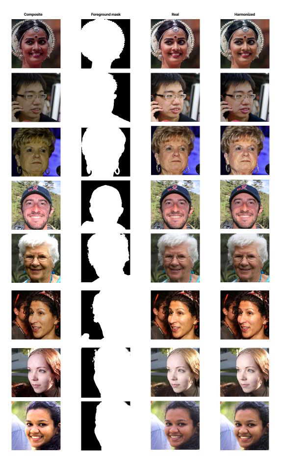
Figure 7: FFHQH dataset. The right column demonstrates PHNet results.

References

- [1] Cao, J., Cong, W., Niu, L., Zhang, J., Zhang, L.: Deep image harmonization by bridging the reality gap (2022)
- [2] Chen, H., Gu, Z., Li, Y., Lan, J., Meng, C., Wang, W., Li, H.: Hierarchical dynamic image harmonization. In: ACM Multimedia (2023)
- [3] Chen, J., Zhang, Y., Zou, Z., Chen, K., Shi, Z.: Dense pixel-to-pixel harmonization via continuous image representation. IEEE Transactions on Circuits and Systems for Video Technology p. 1–1 (2024). https://doi.org/10.1109/tcsvt.2023.3324591, http://dx.doi.org/10.1109/TCSVT.2023.3324591
- [4] Chen, X., Liang, C., Huang, D., Real, E., Wang, K., Liu, Y., Pham, H., Dong, X., Luong, T., Hsieh, C.J., Lu, Y., Le, Q.V.: Symbolic discovery of optimization algorithms (2023)
- [5] Chicherin, S., Efremyan, K.: Adversarially-guided portrait matting (2023)
- [6] Cong, W., Niu, L., Zhang, J., Liang, J., Zhang, L.: BargainNet: Background-guided domain translation for image harmonization. In: ICME (2021)
- [7] Cong, W., Tao, X., Niu, L., Liang, J., Gao, X., Sun, Q., Zhang, L.: High-resolution image harmonization via collaborative dual transformations (2022)
- [8] Cong, W., Zhang, J., Niu, L., Liu, L., Ling, Z., Li, W., Zhang, L.: Dovenet: Deep image harmonization via domain verification. In: CVPR (2020)
- [9] Guo, Z., Gu, Z., Zheng, B., Dong, J., Zheng, H.: Transformer for image harmonization and beyond. IEEE Transactions on Pattern Analysis and Machine Intelligence (2022)
- [10] Guo, Z., Zheng, H., Jiang, Y., Gu, Z., Zheng, B.: Intrinsic image harmonization. In: Proceedings of the IEEE/CVF Conference on Computer Vision and Pattern Recognition (CVPR). pp. 16367–16376 (June 2021)
- [11] Hu, J., Shen, L., Albanie, S., Sun, G., Wu, E.: Squeeze-and-excitation networks (2019)
- [12] Jiang, Y., Zhang, H., Zhang, J., Wang, Y., Lin, Z., Sunkavalli, K., Chen, S., Amirghodsi, S., Kong, S., Wang, Z.: Ssh: A self-supervised framework for image harmonization (2021)
- [13] Karras, T., Laine, S., Aila, T.: A style-based generator architecture for generative adversarial networks (2019)
- [14] Ke, Z., Sun, C., Zhu, L., Xu, K., Lau, R.W.H.: Harmonizer: Learning to perform white-box image and video harmonization (2022)
- [15] Konstantin Sofiiuk, Polina Popenova, A.K.: Foreground-aware semantic representations for image harmonization. arXiv preprint arXiv:2006.00809 (2020)
- [16] Ling, J., Xue, H., Song, L., Xie, R., Gu, X.: Region-aware adaptive instance normalization for image harmonization. In: Proceedings of the IEEE/CVF Conference on Computer Vision and Pattern Recognition. pp. 9361–9370 (2021)
- [17] Loshchilov, I., Hutter, F.: Decoupled weight decay regularization (2019)
- [18] Martino, J., Facciolo, G., Llopis, E.: Poisson image editing. Image Processing On Line 5, 300–325 (11 2016). https://doi.org/10.5201/ipol.2016.163
- [19] Pitie, F., Kokaram, A.: The linear monge-kantorovitch linear colour mapping for example-based colour transfer. In: 4th European Conference on Visual Media Production. pp. 1–9 (2007). https://doi.org/10.1049/cp:20070055
- [20] Pitié, F., Dahyot, R.: N-dimensional probability density function transfer and its application to colour transfer. vol. 2, pp. 1434 – 1439 Vol. 2 (11 2005). https://doi.org/10.1109/ICCV.2005.166
- [21] Reinhard, E., Adhikhmin, M., Gooch, B., Shirley, P.: Color transfer between images. IEEE Computer Graphics and Applications 21(5), 34–41 (2001). https://doi.org/10.1109/38.946629
- [22] Shen, X., Zhang, J., Chen, J., Bai, S., Han, Y., Wang, Y., Wang, C., Liu, Y.: Learning global-aware kernel for image harmonization (2023)
- [23] Song, S., Zhong, F., Qin, X., Tu, C.: Illumination Harmonization with Gray Mean Scale, pp. 193–205 (10 2020). https://doi.org/10.1007/978-3-030-61864-3_17
- [24] Sunkavalli, K., Johnson, M.K., Matusik, W., Pfister, H.: Multi-scale image harmonization. ACM Transactions on Graphics (Proc. ACM SIGGRAPH) 29(4) (2010)
- [25] Tan, L., Li, J., Niu, L., Zhang, L.: Deep image harmonization in dual color spaces. In: Proceedings of the 31st ACM International Conference on Multimedia. MM ’23, ACM (Oct 2023). https://doi.org/10.1145/3581783.3612404, http://dx.doi.org/10.1145/3581783.3612404
- [26] Tao, M.W., Johnson, M.K., Paris, S.: Error-tolerant image compositing. In: European Conference on Computer Vision (ECCV) (2010), http://graphics.cs.berkeley.edu/papers/Tao-ERR-2010-09/
- [27] Valanarasu, J.M.J., Zhang, H., Zhang, J., Wang, Y., Lin, Z., Echevarria, J., Ma, Y., Wei, Z., Sunkavalli, K., Patel, V.M.: Interactive portrait harmonization (2022)
- [28] Xue, B., Ran, S., Chen, Q., Jia, R., Zhao, B., Tang, X.: Dccf: Deep comprehensible color filter learning framework for high-resolution image harmonization (2022)