Accuracy of the Gross-Pitaevskii Equation in a Double-Well Potential

Abstract

The Gross-Pitaevskii equation (GPE) in a double well potential produces solutions that break the symmetry of the underlying non-interacting Hamiltonian, i.e., asymmetric solutions. The GPE is derived from the more general second-quantized Fock Schr$\ddot{\mathrm{o}}$dinger equation (FSE). We investigate whether such solutions appear in the more general case or are artifacts of the GPE. We use two-mode analyses for a variational treatment of the GPE and to treat the Fock equation. An exact diagonalization of the FSE in dual-condensates yields degenerate ground states that are very accurately fitted by phase-state representations of the degenerate asymmetric states found in the GPE. The superposition of degenerate asymmetrical states forms a cat state. An alternative form of cat state results from a change of the two-mode basis set.

I Introduction

The solution of the Gross-Pitaevskii equation (GPE) is a single-particle function that describes Bose condensation [1]. The equation has had considerable success, perhaps especially in treating atoms in traps. A particularly interesting trap is the double well [2]-[22] which allows tunneling; one can find multiple phenomena, including bifurcations to asymmetric states [4]-[22], self-trapping [2, 5, 8, 9], etc. Symmetry breaking has been observed experimentally in several types of systems [23, 25, 26, 27]. The GPE can be derived from the second-quantized Fock Hamiltonian by replacing the field operator by a classical function. In doing this, one neglects the non-commutation of the field operator as a small effect of order of the inverse number of particles. A possible question about various effects shown by the GPE is whether those same or similar effects also occur in the original Fock Schr$\ddot{\mathrm{o}}$dinger equation (FSE) or are they simply artifacts of the GPE. In this paper we center this question on the nonlinear bifurcations that result in asymmetric quantum condensate states. We ask how those states might also appear in the more general Fock description.

There have been extensions of the GPE from the Fock Hamiltonian applicable to trapped gases, for example, the Hartree-Bogoliubov approximation (HBA) by Fetter [16], Ruprecht et al [17], Griffin[18], Popov[19]; also see the summaries in the book by Pethick and Smith[20]. These treatments replace the field operator with a c-number condensate function $\Psi(x)$ plus a correction operator $\phi(x)$ that represents excitations. This quantity is kept to second order in the Fock Hamiltonian and the resulting quadratic Hamiltonian is diagonalized in terms of Bose excitation operators by solving Bogoliubov equations. Our analysis involves a two-mode approximation to the field operator; we keep all orders of the creation and annihilation operators yielding fourth order tunneling terms (neglected in the HBA) that allow dual condensate states representing asymmetric many-particle states in the Fock eigenstates.

The second quantized Fock Hamiltonian in one dimension (in unitless form) is

$$H=\int dx\Psi^{\dagger}(x)\left[-\frac{\partial^{2}}{\partial x^{2}}+V_{ex}(x)\right]\Psi(x)+\frac{1}{2}\int dxdx^{\prime}\Psi^{\dagger}(x)\Psi^{\dagger}(x{}^{\prime})W(x-x^{\prime})\Psi(x^{\prime})\Psi(x),$$ (1)

with external potential $V_{ex}(x)$, interatomic potential $W(x-x^{\prime})=\eta\delta(x-x^{\prime})$, and $\int dx\Psi^{\dagger}(x)\Psi(x)=\hat{N}$, the number operator. Positions are measured in terms of a length $a,$ and energies in

$$\varepsilon=\frac{\hbar^{2}}{2ma^{2}},$$ (2)

and time in $\hbar/\varepsilon.$ Replace the field operator $\Psi(x)$ by a classical variable $\Phi(x)$ to find the energy

$$E=\int dx\Phi^{*}(x)\left[-\frac{\partial^{2}}{\partial x^{2}}+V_{ex}(x)+\frac{\eta}{2}\left|\Phi(x)\right|^{2}\right]\Phi(x),$$ (3)

where $\int dx\left|\Phi(x)\right|^{2}=N$. The time dependent GPE can be derived by varying the energy with respect to $\Phi^{*}$ to get

$$i\frac{\partial\Phi}{\partial t}=\left(-\frac{\partial^{2}}{\partial x^{2}}+V_{ex}(x)+\eta\left|\Phi\right|^{2}\right)\Phi.$$ (4)

Inserting an exponential time dependence, $\Phi(x,t)=e^{-i\mu t}\sqrt{N}\psi(x),$ yields the time-independent GPE in the form

$$\left[-\frac{d^{2}}{dx^{2}}+V_{ex}(x)+\eta N\left|\psi(x)\right|^{2}\right]\psi(x)=\mu\psi(x),$$ (5)

with $\int dx\left|\psi(x)\right|^{2}=1$.

In a recent article [28] we solved this equation for the “box-delta” potential

$$V_{ex}(x)=\left\{\begin{array}[]{cc}\infty,&\left|x\right|\geq 1\\ \gamma\delta(x),&\left|x\right|<1\end{array}\right.,$$ (6)

for which we found analytic solutions of the equation including bifurcations to asymmetric wave functions. Here we want to test the accuracy of the GPE relative to the FSE by treating the box-delta potential approximately using a two-mode model. Two-mode models have been used extensively in studying Bose-Einstein condensation [2]-[4],[6],[8],[9],[11]-[13] and we will find it useful here as well. We begin with a two-mode variational treatment of the GPE, followed by the same method applied to the FSE.

II Variational treatment of GPE

The two states that make up a variational trial wave function are the lowest two states of the non-interacting single particle Hamiltonian, that is, Eq. (5) with $\eta=0.$ These states are

$$\psi_{0}(x) = A\left(\sin k\left|x\right|+\frac{2k}{\gamma}\cos kx\right),$$ (7)

$$\psi_{1}(x) = \sin\pi x.$$ (8)

In $\psi_{0}$ the wave number $k$ satisfies

$$\tan k=-\frac{2k}{\gamma}.$$ (9)

The energies of these two ideal gas states are, respectively,

$$e_{0} = k^{2},$$

$$e_{1} = \pi^{2}.$$

We take $\gamma=10$ throughout. The trial wave function is

$$\psi(x)=u\psi_{0}(x)+v\psi_{1}(x),$$ (10)

which gives energy

$$E=u^{2}e_{0}+v^{2}e_{1}+\frac{\eta N}{2}\left(\chi_{40}u^{4}+\chi_{04}v^{4}+6\chi_{22}u^{2}v^{2}\right),$$ (11)

where

$$\chi_{nm}=\int dx\psi_{0}^{n}(x)\psi_{1}^{m}(x).$$ (12)

With interactions, the symmetric state ($u=1)$ is the lowest energy until $\eta N\leq-2.3$ at which point a superposition of symmetric and antisymmetric states has lower energy, forming an asymmetric state. The asymmetric state has its main peak on one or the other side of the double well (see Fig 1). In the exact calculation of Ref. [28] the bifurcation point is at $\eta N=-2.07$. Fig 1 shows the energy as a function of $\eta N$ in both the exact and variational treatments.

This trial wave function gives a second (degenerate) asymmetric solution as well, with $v$ now having the opposite sign from the first case and main peak on the opposite side.

      

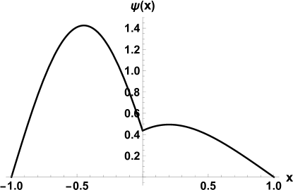
Figure 1: [Left] Asymmetrical variational wave function for $\gamma=10$ and $\eta N=-4.2$ with variational parameter $u=0.8615.$ [Right] Bifurcation to asymmetric states: (Dashed line) The exact energy per particle as a function of interaction $\eta N$ for the symmetric state, and (solid line) the exact asymmetric state. (Dotted line–barely above the exact dashed line) the variational symmetric state; and (dash-dotted line) that for the asymmetric state. The variational bifurcation occurs at $\eta N=-2.3$ compared to the exact result [28] at $-2.07.$

III Two-mode treatment of the Fock Hamiltonian

To test the accuracy of the GPE in producing asymmetric states, we treat the full FSE, also by the two-mode method.

III.1 The energies

In the Fock Hamiltonian of Eq. (1), we substitute the field operator

$$\Psi(x)=a_{0}\psi_{0}(x)+a_{1}\psi_{1}(x),$$ (13)

with $a_{i}$ the annihilation operator for particles in the state $i$. We take matrix elements of the Hamiltonian in the occupation states $\left|n_{0},n_{1}\right\rangle$. The diagonal part of the energy is

$$\frac{H_{0}}{N}=\varepsilon_{0}\frac{n_{0}}{N}+\varepsilon_{1}\frac{n_{1}}{N}+\frac{\eta N}{2}\frac{1}{N^{2}}\left[\chi_{40}n_{0}\left(n_{0}-1\right)+\chi_{04}n_{1}\left(n_{1}-1\right)+4\chi_{22}n_{0}n_{1}\right]$$ (14)

with

$$n_{0}+n_{1}=N.$$ (15)

There is also an off-diagonal part of the Hamiltonian, which is

$$\frac{H^{\prime}}{N}=\frac{\eta N}{2}\frac{\chi_{22}}{N^{2}}\left(a_{0}^{\dagger 2}a_{1}^{2}+a_{1}^{\dagger 2}a_{0}^{2}\right).$$ (16)

This connects states $\left|n_{0},n_{1}\right\rangle$ with $\left|n_{0}+2,n_{1}-2\right\rangle$ and $\left|n_{0}-2,n_{1}+2\right\rangle$. As we will see it is this term that allows the existence of many-body dual condensate states that are the equivalent of the asymmetric states in the solution of the GPE.

We proceed in two steps, first treating just the diagonal energy, and then including the off-diagonal terms as well. In these calculations we take $N=100.$ Minimizing the diagonal terms of Eq. (14) with respect to $n_{0}$ to introduce the possibility of having two condensates, we find that for $\eta N>-4.1$ all the particles condense into the symmetric state; however for $\eta N<-4.1$ a dual condensate has lower energy. This is shown in Fig. 2 in the symmetric state energy and the dual-condensate diagonal energy.

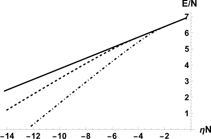
Figure 2: Energies per particle for the Fock Hamiltonian with $N=100$: (Solid line) Energy per particle of a single condensate in the symmetric state versus $\eta N$ [Eq. (14) with $n_{0}=N$, $n_{1}=0$]. (Dashed line) Energy per particle for a dual condensate in the two lowest states using only the diagonal energy of Eq. (14). (Dash-dotted line) Energy per particle for the exact diagonalization of the Hamiltonian in dual condensate states including the tunneling term of Eq. (16). The energy per particle calculated using the GPE is almost identical to this energy.

The off-diagonal tunneling term mixes the dual condensate states to give a wave function of the form

$$\Gamma\left(n\right)=\sum_{n}C_{n}\left|n,N-n\right\rangle.$$ (17)

Because of the quartic nature of the tunneling, states of odd $n$ will be connected to other odd $n$ states and even are connected to even. If the interaction satisfies $\eta N<-2.1,$ the energy now becomes lower than both the symmetric state and the diagonal energy, and we then have a superposition of dual condensates. We also find that the lowest states of the full Fock Hamiltonian are doubly degenerate. The plot of this lowest energy is shown as the dash-dotted curve in Fig. 2.

It is interesting to compare the GPE asymmetric variational energy of Fig. 1 (dash-dotted curve) with the Fock energy of Fig. 2 (dash-dotted curve); it is almost exactly the same, which seems a remarkable coincidence, since the Fock Hamiltonian has so much extra physics, including dual condensates and tunneling.

III.2 The states

When the interaction is sufficiently negative one gets dual condensate states of the form of Eq. (17) and the lowest energy is degenerate. This is certainly reminiscent of the bifurcation in the GPE, in which asymmetric degenerate states became those with the lowest energy. But what are the states here? We pick a particular interaction parameter $\eta N=-4.2$ with $N=50.$ The energy per particle is 5.34. The two states corresponding to this energy are shown in Fig. 3. At first glance the two seem identical, however, the first has all coefficients $C_{n}$ with odd $n$ vanishing, while the second has those with even $n$ vanishing. The two states are clearly orthogonal.

      

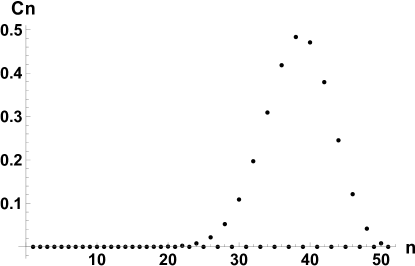
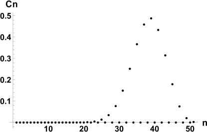
Figure 3: Eigenfunctions of the Fock Hamiltonian for $N=50$ at $\eta N=-4.2.$ The two states are degenerate ground states with energy per particle 5.34. The first (left, call it $\Phi_{a}$), has all coefficients $C_{n}$ with $n$ odd vanishing, while the second (right, $\Phi_{b}$, ) has $C_{n}$ with $n$ even vanishing.

It is useful to compute the one-body density matrix (OBDM) for these states. From the equation

$$\rho_{1}=\left\langle a_{i}^{\dagger}a_{j}\right\rangle$$ (18)

with wave functions of the form of Eq. (17) we have the matrix elements

$$\left\langle a_{0}^{\dagger}a_{0}\right\rangle = \sum_{n}\left|C_{n}\right|^{2}n;\quad\left\langle a_{1}^{\dagger}a_{1}\right\rangle=\sum_{n}\left|C_{n}\right|^{2}\left(N-n\right);$$

$$\left\langle a_{0}^{\dagger}a_{1}\right\rangle = \sum_{n}C_{n+1}^{*}C_{n}\sqrt{\left(n+1\right)\left(N-n\right)};$$

$$\left\langle a_{1}^{\dagger}a_{0}\right\rangle = \sum_{n}C_{n-1}^{*}C_{n}\sqrt{n\left(N-n+1\right)}.$$ (19)

Clearly, if alternating coefficients vanish, $\rho_{1}$ is diagonal and the state can be fragmented. This is the case for the wave functions shown in Fig. 3. We find for each of these two the result

$$\rho_{1}=\left[\begin{array}[]{cc}38.42&0\\ 0&11.58\end{array}\right].$$ (20)

Indeed each state is fragmented and the natural orbitals are the symmetric and antisymmetric basis states.

However these states are not the only basis set possible and it is useful to see whether we can find “pure states,” that is, states that have nearly 100% condensate occupancy. We used Mathematica to diagonalize the Hamiltonian and that has some mechanism built in that provides the particular basis used with degenerate states. Call the states produced there $\Phi_{a}$ and $\Phi_{b}$, as shown in Fig. 3. Then we can produce a new basis set for this ground state by a rotation through angle $\theta$:

$$\Psi_{1} = \Phi_{a}\cos\theta+\Phi_{b}\sin\theta,$$

$$\Psi_{2} = \Phi_{a}\sin\theta-\Phi_{b}\cos\theta.$$ (21)

We choose $\theta$ to maximize the condensate number in a single state. We find by trial new states with $\theta=0.78540$ that have the largest OBDM eigenvalues. These states are shown in Fig. 4. The OBDMs are now given by

$$\rho_{1}=\left[\begin{array}[]{cc}38.42&\pm 21.08\\ \pm 21.08&11.58\end{array}\right]$$ (22)

with eigenvalues

$$N_{1} = 49.987,$$

$$N_{2} = 0.013.$$ (23)

      

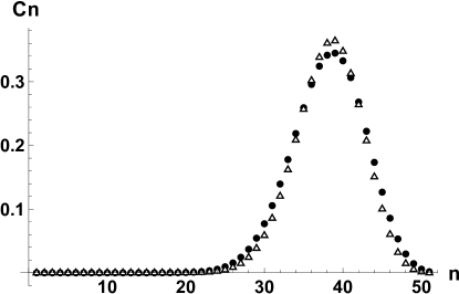
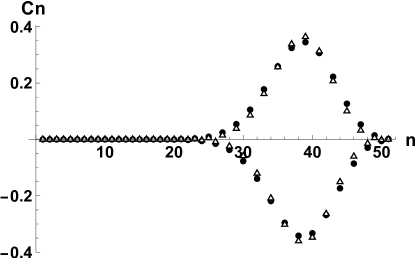
Figure 4: Rotated states (Black dots): States (left: $\Psi_{1}$ and right: $\Psi_{2}$) that are linear combinations [Eq. (21)] of the degenerate ground states of the Fock Hamiltonian, chosen to make the largest single condensates. (Open triangles): Fitted coefficients Eqs.(26) and (27) of pure condensate asymmetric states.

If the numerical states shown are related to the basic asymmetric condensate states found with the GPE, then we should be able to fit them with binomial coefficients generated from the pure asymmetric state and its mirror image:

$$\xi_{+} = \frac{1}{\sqrt{N!}}(ua_{0}^{\dagger}+va_{1}^{\dagger})^{N}\left|0\right\rangle,$$ (24)

$$\xi_{-} = \frac{1}{\sqrt{N!}}(ua_{0}^{\dagger}-va_{1}^{\dagger})^{N}\left|0\right\rangle,$$ (25)

with $\upsilon=\sqrt{1-u^{2}}.$ (These are asymmetrical because the single-particle state $(ua_{0}^{\dagger}\pm va_{1}^{\dagger})$ is a sum of a symmetric and an antisymmetric wave function.) These two states are nearly orthogonal; we will discuss this aspect below. When expanded the coefficients in each are, respectively,

$$D_{n}^{+} = \sqrt{\frac{N!}{n!(N-n)!}}u^{n}v^{N-n},$$ (26)

$$D_{n}^{-} = \sqrt{\frac{N!}{n!(N-n)!}}u^{n}(-v)^{N-n}.$$ (27)

We compare these forms with the numerical plots in Fig. 4 in the open triangles where a least square fit gives $u=0.87653$. The fit is good but not exact. The energies $E/N$ of the states are as follows:Mathematica states [Fig. 3] : 5.3391; the fitting states $\xi_{\pm}$: 5.3402, which is a bit higher, as it should be. It is interesting that the condensate [Eq. (23)] is not pure; there seems to be a small occupation of an excited state. This state, with the same $u$ and $v$, is

$$\xi_{3}=\frac{1}{\sqrt{N!}}(va_{0}^{\dagger}-ua_{1}^{\dagger})^{N}\left|0\right\rangle.$$ (28)

This state is orthogonal to $\xi_{+}$ and has energy 6.874; it is an excited state. The coefficients corresponding to this state oscillate like the right plot of Fig. 4, but with the peak at small $n=12$ rather than large $n$.

What we have shown here is that the states of Eqs. (24) and (25), which represent degenerate condensates in asymmetric states, are eigenfunctions of the Fock Hamiltonian in the two-modes approximation. As such this feature is reminiscent of what occurs in the GPE.

III.3 The fitting parameters

We found values of the rotation angle $\theta$ and the value of $u$ that allowed a fit of the least-fragmented states. Let’s see why we got the numbers we did. States like Eqs. (24) and (25) in the form

$$\left|u,v,N\right\rangle=\frac{1}{\sqrt{N!}}(ua_{0}^{\dagger}+va_{1}^{\dagger})^{N}\left|0\right\rangle$$ (29)

are phase states. (If $u=\left|u\right|e^{i\phi_{u}}$ and $v=\left|v\right|e^{i\phi_{v}}$, then the “phase” is $\phi=\phi_{v}-\phi_{u}$.) Phase states with different phases become orthogonal when $N\rightarrow\infty$ [29]. In the case of $\xi_{+}$ and the mirror state $\xi_{-}$ we find that $\left\langle\xi_{+}|\xi_{-}\right\rangle=(u^{2}-v^{2})^{N}=3\times 10^{-14}$. On the other hand, the numerical states that we generated are exactly orthogonal. A phase state is a kind of eigenfunction of the destruction operator [29]:

$$a_{0}\left|u,v,N\right\rangle = u\sqrt{N}\left|u,v,N-1\right\rangle,$$ (30)

$$a_{1}\left|u,v,N\right\rangle = v\sqrt{N}\left|u,v,N-1\right\rangle.$$ (31)

With these equations it is easy to show that the OBDMs of $\xi_{\pm}$ are

$$\rho_{\pm}=N\left[\begin{array}[]{cc}u^{2}&\pm uv\\ \pm uv&v^{2}\end{array}\right].$$ (32)

Numerically, Mathematica found Eq. (22) so that comparison with Eq. (32) gives $Nu^{2}=38.42$ or that $u=0.8766.$ The least squares fit gave $0.87653$.

The transformation Eqs. (21) between states is unitary, so that, if our original $Mathematica$ Fock states are $\Phi_{a}$ and $\Phi_{b}$, we can write

$$\Phi_{a} \approx \xi_{+}\cos\theta+\xi_{-}\sin\theta,$$

$$\Phi_{b} \approx \xi_{+}\sin\theta-\xi_{-}\cos\theta.$$ (33)

But from Eqs. (26) and (27) we see that the simple sum $\xi_{+}+\xi_{-}$ will have odd numbered coefficients vanishing, while the difference $\xi_{+}-\xi_{-}$will have even numbered coefficients zero. That implies $\cos\theta=\sin\theta$ or $\theta=\frac{\pi}{4}=0.785398$ whereas our minimization of the small condensate led to $0.78540$.

III.4 A peculiar condensate

A condensate of the general form of that of Eq. (24) is rather standard: all $N$ particles are in the same single-particle state. In this case that state is a superposition of two other states and it appears to the $N$th power. The state represented by the OBDM of Eq. (20) is fragmented with 38 particles in the ground symmetric state $\psi_{0}$ [Eq. (7)] and 12 in the antisymmetric states $\psi_{1}$[Eq. (8)]. However, the dual condensation is not in the state $\left|n_{0},n_{1}\right\rangle=\left|38,12\right\rangle,$ but is in a superposition of $\left|0,50\right\rangle$, $\left|2,48\right\rangle,$$\cdots$$\left|50,0\right\rangle$ with varying coefficients. This form of fragmentation is not original to this paper; for example, it appears in Refs. [7], [30], and [31] but we thought the form unusual enough to be worth pointing out.

III.5 Cat states

The states $\Psi_{1}$ and $\Psi_{2}$ of Eqs. (21), given their approximation by $\xi_{+}$ and $\xi_{-}$, are made up of states localized mostly on one side of the double well or the other ($ua_{0}^{\dagger}\pm va_{1}^{\dagger})$. As such, their sum

$$\Psi_{+}=\frac{1}{\sqrt{2}}\left(\Psi_{1}+\Psi_{2}\right)$$ (34)

is a sum of macroscopically distinct states and so qualifies as a “cat state”. Its two components are orthogonal to one another and so the cat state has the same energy as each of the degenerate components. Ref. [10] also considered the possibility of constructing a cat state out of asymmetrically localized states of the GPE.

There is another type of cat state that can be considered here, namely a cat state in double-condensate space; that is, those that have double peaks in the distribution of coefficients $C_{n}$ in the states of the form of Eq. (17). These have been considered in, for example, Refs. [7, 30, 31]. When we expanded the Fock state in a two-mode approximation we used the ground $\psi_{0}$ and first excited state $\psi_{1}$ of the non-interacting potential. We found these resulted in combinations that involved asymmetric states. Suppose we expand directly in asymmetric states by considering the basis

$$\psi_{+} = \frac{1}{\sqrt{2}}\left(\psi_{0}+\psi_{1}\right),$$ (35)

$$\psi_{-} = \frac{1}{\sqrt{2}}\left(\psi_{0}-\psi_{1}\right).$$ (36)

These functions are plotted in Fig. 5; they are clearly asymmetric. However, they are also orthogonal unlike most asymmetric mirror functions.

      

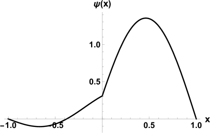
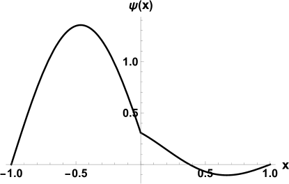
Figure 5: The states corresponding to Eqs. (35) and (36): (Left) $\psi_{+}=(\psi_{0}+\psi_{1})/\sqrt{2}$; (Right) $\psi_{-}=(\psi_{0}-\psi_{1})/\sqrt{2}$.

The operators corresponding to these states are

$$a_{+} = \frac{1}{\sqrt{2}}\left(a_{0}+a_{1}\right),$$ (37)

$$a_{-} = \frac{1}{\sqrt{2}}\left(a_{0}-a_{1}\right)..$$ (38)

Suppose we make a transformation from dual condensate states $\left|n,N-n\right\rangle_{01}$ to $\left|m,N-m\right\rangle_{\pm}$, corresponding respectively to $\left\{a_{0},a_{1}\right\}$ and $\left\{a_{+},a_{-}\right\}$ so that the wave function is

$$\Psi=\sum_{n}C_{n}\left|n,N-n\right\rangle_{01}=\sum_{m}B_{m}\left|m,N-m\right\rangle_{\pm},$$ (39)

where

$$B_{m}=\sum_{n}A_{mn}C_{n}.$$ (40)

The transformation matrix is found to be

$$A_{mn}=\frac{1}{2^{N/2}}\sum_{k}\frac{\sqrt{n!m!(N-n)!(N-m)!}(-1)^{N-n-m+k}}{k!(n-k)!(m-k)!(N-n-m+k)!},$$ (41)

where the sum on $k$ (because of the factorials) goes from $\max(0,n+m-N)$ to $\min(n,m).$ When we apply this transformation to the states we found in Sec. III.2, i.e., those shown in Fig. 3, we find the double-peaked cat states shown in Fig. 6.

      

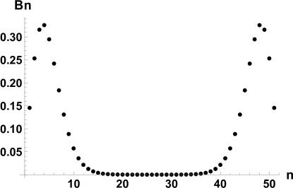
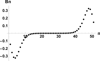
Figure 6: Cat states in dual-condensate space gotten by transforming from the $\left\{a_{0},a_{1}\right\}$ basis to the $\left\{a_{+},a_{-}\right\}$ basis of Eqs. (37) and (38).

We can say a bit more about the peaks in the cat states shown here. Suppose we expand the state of Eq. (24) in the set $\left\{a_{+},a_{-}\right\}$ by using the transformations of Eqs. (37) and (38). With $u=0.877$ that corresponded approximately to an asymmetric eigenstate of the Fock Hamiltonian at $\eta N=-4.2$. Plotting the expansion coefficient of Eq. (24) in the set $\left\{a_{+},a_{-}\right\}$ produces the right-most peak of the cat state. When we expand Eq.(25) we get the left-most peak of the cat. Thus each peak represents one of the many-body asymmetric states found with the Fock Hamiltonian.

Reference [7] showed that if one made measurements one particle at a time where each measurement determined which of the condensate states the particle occupied, in this case $\psi_{+}$ or $\psi_{-}$, then after a rather small number of measurements the cat state would collapse to just one of the peaks. Is such a cat state, in this case involving asymmetric states, more capable of being formed than other kinds? Could asymmetric states aid in making cat states?

IV Self-consistent dual condensates

Cederbaum and coworkers [32] (and others [4, 5]) have derived self-consistent equations for systems of multicomponent condensates, called the multi-configurational Hartree theory for bosons (MCHB). Originally they derived equations from just the diagonal terms in the Fock Hamiltonian, but later generalized that to use all the terms, including off-diagonal tunneling terms. The single-condensate version of MCHB is just the GPE itself. In our two-mode approximation for the two-condensate Fock Hamiltonian we kept the trial states the same, the symmetric and antisymmetric lowest states of the noninteracting potential. In MCHB, the states will change with each change of interaction parameter and in some cases might become asymmetric states themselves. A further interesting study would be to consider this type of two-mode analysis and its connection to the asymmetric states. The MCHB method is capable of treating more than two condensate states as well. We reserve such studies for future work.

V Discussion

We have used a two-mode analysis to compare results derived from the Fock Hamiltonian to the results using just the GPE. As preparation, we made a two-mode variational treatment of asymmetric states in the box-delta potential, which are a reasonably accurate representation of the bifurcation to the asymmetric states for sufficiently negative interaction parameter $\eta N.$ The states are pair degenerate with the wave function peak on one side of the well or the other.

The GPE yields a single-condensate wave function function, having an asymmetric solution with a degenerate mirror function. In the two-mode treatment of the Fock $H$, it becomes possible to have dual condensate states. In terms of these states, of the form $\left|n\right\rangle\equiv\left|n,N-n\right\rangle$, there is a diagonal energy as well as an off-diagonal energy representing tunneling between the $\left|n\right\rangle$ states. The use of just the diagonal energy leads to a single energetically preferred dual state $\left|n\right\rangle$ favored over the symmetric single condensate state below a critical negative interaction strength. However, inclusion of the tunneling leads to states of the form $\sum_{n}C_{n}\left|n\right\rangle$, i.e., superpositions of dual condensates states. Below a critical interaction parameter value, the states initially produced by the numerical method used have alternating $C_{n}$ values vanishing either with odd $n$ or with even $n.$ These two states are degenerate and have one-body density matrices that are diagonal with fragmented condensates in the original symmetric and antisymmetric states. These condensates involve superpositions of odd (or even) numbers of particles in each of the two basis states. In another representation the asymmetric states are the natural orbitals with almost all particles falling into one of those states or the other. There is a small depletion there with a 0.03% occupation of another state. Our results demonstrate that the GPE yields a quite accurate representation of the more general Fock Schr$\ddot{\mathrm{o}}$dinger equation, with asymmetry occurring in a very similar form in each.

Of the numerical states approximated by $\xi_{+}$ and $\xi_{-}$, one is physically localized more on one side of the well; the opposite on the other side. The sum of these, one of the states in Fig. 3, is a cat state, a sum of two macroscopically distinct states; but one of precisely the same energy as that of each of the two components, since the components are orthogonal. A more interesting cat state was found in dual-condensate space by changing the basis set of the two-mode analysis. However, it is not clear how asymmetric states could be used to form cat states experimentally.

VI Acknowledgement

We thank Karen Lord for a helpful conversation.

References

- [1] Franco Dalfovo, Stefano Giorgini, Lev P. Pitaevskii, and Sandro Stringari, “Theory of Bose-Einstein condensation in trapped gases,” Rev. Mod. Phys. 71, 463 (1999).
- [2] G. J. Milburn, J. Corney, E. M. Wright, D. F. Walls, “Quantum dynamics of an atomic Bose-Einstein condensate in a double-well potential,” Phys. Rev. A 55, 4318 (1997).
- [3] R. W. Spekkens and J. E. Sipe, “Spatial fragmentation of a Bose-Einstein condensate in a double-well potential,” Phys. Rev. A 59, 3868 (1999).
- [4] D. J. Masiello, S. B. McKagan, and W. P, Reinhardt, “Multiconfigurational Hartree-Fock theory for identical bosons in a double well,” Phys. Rev. A 72, 063624 (2005).
- [5] D. J. Masiello and W. P. Reinhardt, “Symmetry-Broken Many-Body Excited States of the Gaseous Atomic Double-Well Bose-Einstein Condensate,” J. Phys. Chem. A 123, 1962 (2019).
- [6] S. Raghavan, A. Smerzi, S. Fantoni, and S. R. Shenoy, “Coherent oscillations between two weakly coupled Bose-Einstein condensates: Josephson effects, oscillations, and macroscopic quantum self-trapping,” Phys. Rev. A 59, 620 (1999).
- [7] W. J. Mullin, A. R. Sakhel, and R. J. Ragan, “Progressive quantum collapse,” Amer. J. Phys. 90, 200 (2022).
- [8] E. A. Ostrovskaya, Y. S. Kivshar, M. Lisak, B. Hall, F. Cattani, and D. Anderson, “Coupled-mode theory for Bose-Einstein condensates,” Phys. Rev. A 61, 031601(R) (2000).
- [9] P. Coullet and N. Vandenberghe, “Chaotic self-trapping of a weakly irreversible double Bose condensate,” Phys. Rev. E 64, 025202(R) (2001).
- [10] K. W. Mahmud, J. N. Kutz, and W. P. Reinhardt, “Bose-Einstein condensates in a one-dimensional double square well: Analytical solutions of the nonlinear Schrdinger equation,” Phys. Rev. A 66, 063607 (2002).
- [11] J. Adriazola, R. H. Goodman, and P. G. Kevrekidis, “Efficient Manipulation of Bose-Einstein Condensates in a Double-Well Potential,” Commun Nonlinear Sci Numer Simululat 122, 107219 (2023).
- [12] G. Theocharis, P. G. Kevrekidis, D. J. Frantzeskakis, and P. Schmelcher, “Symmetry breaking in symmetric and asymmetric double wells,” Phys. Rev. E 74, 056608 (2006).
- [13] A. Smerzi, S. Fantoni, S. Giovanazzi, and S. R. Shenoy, “Quantum Coherent Atomic Tunneling between Two Trapped Bose-Einstein Condensates,” Phys. Rev. Lett. 79, 4950 (1997).
- [14] Roberto D’Agosta and Carlo Presilla, “States without a linear counterpart in Bose-Einstein condensates,” Phys. Rev. A 65, 043609 (2002).
- [15] R. K. Jackson and M. I. Weinstein, “Geometric Analysis of Bifurcation and Symmetry Breaking in a Gross-Pitaevskii Equation,” J. Stat. Phys. 116, 881 (2004).
- [16] A. L. Fetter, “Nonuniform States of an Imperfect Bose Gas,” Ann. Phys. (N.Y.)70, 67 (1972); “Ground state and excited states of a confined condensed Bose gas,” Phys. Rev. A 53, 4245 (1996); A. L. Fetter and J. D. Walecka, (McGraw-Hill, New York, 1971), Chaps 2, 10, 14.
- [17] P. A. Ruprecht, Mark Edwards, K. Burnett, and Charles W. Clark, “Probing the linear and nonlinear excitations of Bose-condensed neutral atoms in a trap,” Phys. Rev. A 54, 4178 (1996); R. J. Dodd, M. Edwards, C. J. Williams, C. W. Clark, P. A. Ruprecht, and K. Burnett, “Zero-Temperature, Mean-Field Theory of Atomic Bose-Einstein Condensates”, J. Res. Nat. Inst. Stand. Tech. 101, 553 (1996).
- [18] A. Griffin, “Conserving and gapless approximations for an inhomogeleous Bose gas at finite temperatures,” Phys.Rev. B 51, 9341 (1996).
- [19] V. N. Popov, , (CambridgeUnifv. Press, Cambridge, 1987).
- [20] C. J. Pethick and H. Smith, , Cambridge Univ. Press 2002, Chaps.7 and 8.
- [21] B. A. Malomed, ed. “Spontaneous Symmetry Breaking, Self-Trapping, and Josephson Oscillations, Springer -Verlag: Berlin and Heidelberg, 2013.
- [22] Elad Shamitz, Nir Dror, and Boris A. Malomed, “Spontaneous Symmetry Breaking in a split potential box,” Phys. Rev. E 94, 022211 (2016); Boris A. Malomed, “Spontaneous Symmetry Breaking in Nonlinear Systems: an Overview and a Simple Model,” in “Nonlinear Dynamics: Materials, Theory, and Experiments,” eds. M. Tlidi and M. Clerk, pp. 97-112 Springer-Heidelberg 2016 and arXiv:1511.08340v1 [nlin.PS]; “Symmetry breaking in laser cavities,” Nature Photonics 9, 287 (2015).
- [23] C. Green, G. B. Mindlin, E. J. D’Angelo, H. G. Solari, and J. R. Tredicce, “Spontaneous Symmetry Breaking in a Laser: The Experimental Side,” Phys. Rev. Lett, 65, 3124 (1990).
- [24] C. Cambournac, T. Sylvestre, H. Maillotte, B. Vanderlinden, P. Kockaert, Ph. Emplit, and M. Haelterman, “Symmetry-Breaking Instability of Multimode Vector Solitons,” Phys. Rev. Lett. 89, 083901 (2002).
- [25] P. G. Kevrekidis, Zhigang Chen, B. A. Malomed, D. J. Frantzeskakis, and M. I. Weinstein, “Spontaneous symmetry breaking in photonic lattices: Theory and experiment,” Phys. Lett. A 340, 275-280 (2005).
- [26] Philippe Hamel, Samir Haddadi, Fabrice Raineri, Paul Monnier, Gregoire Beaudoin, Isabelle Sagnes, Ariel Levenson and Alejandro M. Yacomotti, “Spontaneous mirror-symmetry breaking in coupled photonic-crystal nanolasers,” Nature Photonics 9, 311 (2015).
- [27] Tilman Zibold, Eike Nicklas, Christian Gross, and Markus K. Oberthaler, “Classical Bifurcation at the Transition from Rabi to Josephson Dynamics,” Phys. Rev. Lett. 105, 204101 (2010).
- [28] R. J. Ragan. A. R. Sakhel, and W. J. Mullin, “ The Gross-Pitaevskii equation for an infinite square-well with a delta-function barrier,” arXiv:2401.13833[quant-ph]
- [29] W. J. Mullin, R. Krotkov, and F. Lalo, “The origin of the phase in the interference of Bose-Einstein condensates,” Am. J. Phys. 74, 880 (2006).
- [30] Erich J. Mueller, Tin-Lun Ho, Masahito Ueda, and Gordon Baym, “Fragmentation of Bose-Einstein Condensates,” Phys. Rev. A 74, 033612 (2006).
- [31] T.-L. Ho and C. V. Ciobanu, “The Schrdinger Cat Family in Attractive Bose Gases,” J. Low Temp. Phys. 135, 257 (2004).
- [32] L. S. Cederbaum and A. I. Streltsov, “Best mean-field for condensates,” Phys. Lett. A 318, 564 (2003); A. I. Streltsov, O. E. Alon, and L. S. Cederbaum, “General variational many-body theory with complete self-consistency for trapped bosonic systems,” Phys. Rev. A 73, 063626 (2006). O. E. Alon, A. I. Streltsov, and L. S. Cederbaum, “Multiconfigurational time-dependent Hartree method for bosons: Many-body dynamics for bosonic systems,” Phys. Rev. A 77, 033613 (2008).