The optimizing mode classification stabilization of sampled stochastic jump systems via an improved hill-climbing algorithm based on Q-learning
Abstract
This paper addresses the stabilization problem of stochastic jump systems (SJSs) closed by a generally sampled controller. Because of the controller’s switching and state both sampled, it is challenging to study its stabilization. A new stabilizing method deeply depending on the mode classifications is proposed to deal with the above sampling situation, whose quantity is equal to a Stirling number of the second kind. For the sake of finding the best stabilization effect among all the classifications, a convex optimization problem is developed, whose globally solution is proved to be existent and can be computed by an augmented Lagrangian function. More importantly, in order to further reduce the computation complexity but retaining a better performance as much as possible, a novelly improved hill-climbing algorithm is established by applying the Q-learning technique to provide an optimal attenuation coefficient. A numerical example is offered so as to verify the effectiveness and superiority of the methods proposed in this study.
Index Terms:
Stochastic jump systems; sampled control; mode classification and optimization; Lagrangian function; hill-climbing algorithm; Q-learning.I Introduction
Significantly different from deterministic systems, stochastic jump system (SJS) can represent physical systems experiencing random structure changes. Due to this system with multiple structures or modes, it makes its stabilization problems quite distinctive whose controller’s quantity is not unique. According to the designed controller depending on mode or not, the existing stabilization results are mainly classified into two categories. The first kind needs the mode of controller to keep pace with others and are usually called to be mode-dependent control method such as [1, 2, 3, 4, 5, 6]. Due to all the modes synchronized with each other at the same time, the effect of stabilization effect will be the best and have the least conservatism. However, this advantage is also its disadvantage which will be limited in practice, since a lot of effort is needed to keep this synchronization all the time. In theoretical research, an ideal assumption for all the mode information available in real time is commonly acquiescent. The second kind is mentioned as mode-independent control approach [7, 8, 9, 10], in which the mode information is totally removed even if it is available sometimes. Because the mode information is totally removed in controller, it can stabilize a system regardless of its mode accessible or not and naturally bring more conservatism. In contrast to mode-dependent control being very ideal, mode-independent control is excessively absolute due to mode information neglected completely. For the purpose of bridging the above methods and balancing their advantages and disadvantages, some improved controllers were developed, such as partially mode-dependent controller [11] and partial information controller [12]. However, the drawbacks of mode-dependent and -independent control methods have not been partly solved, and there are still some problems to be further studied. For example, the quantity of controllers denoted as in the above references is no less than number of modes referred to be . Consequently, an interesting problem about SJSs can be proposed such that whether one can stabilize an SJS using fewer controllers but more than one. In this situation, some results were found, see, e.g., disordered or unmatched controller [13, 14], and scheduling controller [15, 16]. Though the aim of fewer controllers stabilizing an SJS with more subsystems was realized, it can be found from these references that for each subsystem or mode, at most total controllers were added once, while the equipment cost and conservatism of stabilization realizing were both increased. The main reason is that the developed controller in these references was designed on the whole modes without considering them separately. When the controller is designed according to the mode classifications, a quantity limited controller method was in proposed in [17]. However, the mode classification method for designing controllers is not fully studied, and many interesting and significant topics need to be further researched. For example, whether there is an optimization classification or not and how to find the best mode classification will be the first problems, and more extensions based on optimizing mode classification method will also be meaningful.
On the other hand, it is well known that networked control system (NCS) is a control system whose components are connected through a communication network. Though NCS has such advantages, there is a precondition that all the transmitted data should be first sampled. Importantly, the appearance of sampled data complicates system analysis and synthesis and causes many unpredictable problems. It can further bring some negative effects such as communication delays, data packet dropouts and/or packet disordering, network attack, some of which are not easy. Thus, it is very important to research the sampling phenomenon scientifically. Particularly, when an SJS is connected by a network, some novel but hard issues will encounter such that not only state but also switching signal are sampled. Due to switching being stochastic, its sampling is specific and significantly different from state sampled. Accordingly, some interesting but challenging problems emerge. Up to now, very few results are found to study the stabilization of stochastic systems via a sampled-switching controller. On the one hand, the author in [18] first considered its stabilization problem by applying an auxiliary system approach. More extensions [19, 20] were further obtained base in this method. Since the stabilization problem of original sampling system was transformed to study its auxiliary system without any sampling, it decided that the sampling bound should be very small. On the other hand, based on an augmented system method, the stabilization of Markovian jump systems (MJSs) closed by a sampled switching and state controller was studied in [21], whose sampling effect was modeled to be a time-varying exponential matrix. Unfortunately, the convergency guaranteed by the reference was only asymptotically mean stable and was worse than the common stability concepts such as almost surely exponentially stable, globally asymptotically stable and so on. To summarize, it is necessary to further investigate the stabilization problem of sampled stochastic jump systems. Moreover, new approaches are expected to provide larger sampling bounds and better convergency properties. Meanwhile, many difficulties will encounter in the research, some of which are challenging. For example, how to establish a quantized correlation between the original switching and its sampled value will be the first difficulty to encounter, since no more suitable models are available. Particularly, it will be challenging to achieve the above expected objectives, because both switching and state are sampled simultaneously. Especially so many possible combinations of switching and its sampled values will emerge and bring large difficulties in system analysis and synthesis.
The main contributions of this paper are as follows: 1) For the aim of overcoming the control difficulties of sampling in both state and switching signals, a new stabilizing controller is established to be very closed to the mode classifications. On the one hand, the controller’s quantity is smaller than mode-dependent controllers, and its switching is not necessary synchronous to the original one. On the other hand, the conservatism is smaller than mode-independent ones [7, 8, 9, 10]; 2) So as to further improve the stabilization performance, a convex optimization problem is presented to determine the best classification of sampled stabilization, which is better than [17] without mode optimization. It can be shown that the optimal solution can exist and be obtained by computing some equations coming from an augmented Lagrangian function; 3) Due to the classification quantity being a Stirling number of the second kind and large, a novel method having less complexity but better control performance is proposed based on the hill-climbing algorithm by using the Q-learning technique to ensure an optimal attenuation coefficient. Particularly, not only the monotonicity but also the convergency of method in this paper is guaranteed; 4) Compared with the existing auxiliary system approach [18] and augmented system method [21], the developed method is less conservative and has larger sampling bounds. Moreover, the key idea in this paper can popularize in many situations as long as the system switching experiences a sampling or mismatching phenomenon.
Notation , , and represent the sets of real numbers, positive real numbers, non-negative real numbers and positive integers respectively. denotes the n-dimensional Euclidean space, and is a set of vector whose each element is non-negative. and are the probability and expectation operators respectively. refers to the Euclidean vector norm or spectral matrix norm. and denote the smallest and largest eigenvalues of a square matrix , and .
II Problem formulation
Consider a stochastic jump system described as
| (1) |
where , and and . The stochastic switching process is a piecewise constant function and right-continuous. In detail, it is actual the semi-Markvoian switching and takes values from a set such as , , , where switching instant satisfies . For simplicity, at the th switching instant is simply denoted to be .
In contrast to the usual controllers designed for stochastic systems including (1), a general controller with sampling phenomenon is described to be
| (2) |
where is the control gain, is the sampling instant such as , and is denoted as the sampling interval. Obviously, the simultaneous existence of two instant sequences and makes the system analysis and synthesis not easy. Especially, due to being sampled, it will bring large difficulties and also complicates the closed-loop system. The first reason is that so many combinations about original signal and its sampled signal encounter and inevitably result in great complexity and large conservatism. The second reason, but not the last, is that the sampled state existing simultaneously also leads to negative effects such that the correlation between the original and sampled states on each subinterval is hard to be done. In order to solve the above mentioned problems, the controller is developed as
| (3) |
where and are to be designed. Particularly, the sampling instant of controller (3) is different from (2). In detail, the sampling instant of (3) is event-triggered such as
| (4) |
Accordingly, function on interval with property (4) is defined as , when . Meanwhile, set is a newly constructed subset based on and defined as
| (5) |
where , , and constant is the quantity of elements of set and denoted as . Moreover, all the elements of set are mutually exclusive such as
| (6) |
Then, it can be concluded that
| (7) |
where . Moreover, subset can be further expressed as
| (8) |
where , . When the above mentioned classification and event-trigger scheme achieve, controller (3) will be superior to (2), which can be realized easily and of larger significance in theory and practice. Moreover, a mapping between controllers and subsystems or modes should be introduced. In the next, it will be seen that this mapping can not only be used to design a new controller for stochastic systems but also bridge the traditionally mode-dependent and -independent controllers very well.
Remark 1
It is noted that controller (3) includes some existing controllers without any sampling signals as special situations in which neither or is sampled. First of all, when and , , in addition to with but , controller (3) without sampled state but with will be simplified to the traditionally mode-dependent controller such as . Second, under a deterministic classification same to the first situation, and if with , one could get a partial information controller similar to [12]. Moreover, if takes discrete values such as , a disordered controller similar to [13] will be obtained. Thirdly, when there is only one element in such as , there will be only one element in such as . Then, controller (3) with replaced by will reduce to be the traditionally mode-independent controller . When is equal to the stationary distribution, the mode-independent controller will be an optimal estimation of similar to [17, 22].
Though some existing controllers are included as special situations of sampled controller (3), their methods cannot be used to deal with (3). Obviously, controller (3) deeply depends on the mode classification. Meanwhile, so many possible combinations of the division about set are involved whose division value is a positive natural number. Particularly, it can be known from [23] that its value is equal to which is a Stirling number of the second kind and described to be
Its detailed expansion [24] is given to be
| (9) |
When the classification of (3) is not given in advance, controller (3) should deeply depend on the Stirling number of the second kind and be rewritten as
| (10) |
where is selected to be only one value from . Accordingly, the related symbols in definitions (5)-(8) will change to be
Then, two necessary but not easy problems are proposed as follows:
Problem 1: Whether does the best classification of set exist or not?
Problem 2: How to find the best classification to design a sampled stabilizing controller such as (10)?
First of all, a cost function is introduced to be
| (11) |
where matrix is composed of but depends on classification parameter . Then, the related optimization problem is to find the optimal classification and its related optimal classification parameter of sampled controller (10) satisfying
| (12) | ||||
where the optimal solution satisfies . Similarly, one can define such as , where means there is always a controller added to each subsystem. It can be seen from (12) that a normal method getting the solution to Problem 2 is to compute cost function (11) one by one whose process will repeat times. After doing that, one can select the solution minimizing the value of (11) as the globally optimal solution. Obviously, when and become large, the complexity of computation will be very large. Thus, it is necessary to develop a new way which provides a suboptimal solution nearing the globally optimal solution as much as possible but has smaller complexity without computing (11) one by one. In this paper, an improved hill-climbing algorithm (HCA) based on the Q-learning technique will be developed, which can not only avoid traversing all the classifications but also guarantee the proposed algorithm some good properties such as convergence and monotonicity. As a result, the computation complexity will be largely reduced, while the cost function will also have an optimal value. Some fundamentally dealing processes should be established firstly.
First of all, some constants about classification set are needed and important in designing the optimization method to be presented. In detail, each element of is arranged by such as . Meanwhile, all the elements of are rewritten as an ascending sequence such as , since they are natural numbers and distinct from each other. Then, two kind parameters referred to be and about subset can be generated. On the one hand, parameter is generated by arranging every with selecting simultaneously and sequently such as . On the other hand, similar to , parameter is constructed by arranging all the elements of every subset following an ascending sequence such as
Based on these parameters, an one-to-one correlation or mapping between sets and can be obtained by arranging the value of orderly along with the values of and increasing successively. To illustrate the above process clear and vividly, an example about and is given in Table I. There, all the subset classifications about and with are listed followed by the above proposed process, while parameters and are computed too. Without loss of generality, only two situations are discussed in detail. The first situation is , and . Obviously, one knows , and , while and . Because of being the smallest among , and based on the proposed mapping principle, one should select . Similarly, means the second-smallest value of among such as . The second situation is , and . Then, one knows , and , such that and . Though the values of about the two situations are the same, the values of are different. Due to , the values of parameter are different and selected to be and respectively followed by the above mapping. The other situations are all given in Table I, whose detailed computation processes are omitted.
| 113 | 12345 | 1 | |||
| 113 | 13245 | 2 | |||
| 113 | 14235 | 3 | |||
| 113 | 15234 | 4 | |||
| 113 | 23145 | 5 | |||
| 113 | 24135 | 6 | |||
| 113 | 25134 | 7 | |||
| 113 | 34125 | 8 | |||
| 113 | 35124 | 9 | |||
| 113 | 45123 | 10 | |||
| 122 | 12345 | 11 | |||
| 122 | 12435 | 12 | |||
| 122 | 12534 | 13 | |||
| 122 | 21345 | 14 | |||
| 122 | 21435 | 15 | |||
| 122 | 21534 | 16 | |||
| 122 | 31245 | 17 | |||
| 122 | 31425 | 18 | |||
| 122 | 31524 | 19 | |||
| 122 | 41235 | 20 | |||
| 122 | 41325 | 21 | |||
| 122 | 41523 | 22 | |||
| 122 | 51234 | 23 | |||
| 122 | 51324 | 24 | |||
| 122 | 51423 | 25 |
Secondly, after introducing the mapping between sets and , an optimization algorithm based on a local search can be proposed and remain some advantages. In detail, on the one hand, a trajectory only using the selected partial nodes instead of exploiting all the division nodes is generated. In other words, it can lead to a locally even globally optimal solution by an iterating method. On the other hand, a favorable convergence and monotonicity of the proposed algorithm should be satisfied. Particularly, based on the proposed mapping, the normal HCA can be used to realize the former requirement of locally optimal solution. However, the other properties on the convergence and monotonicity described in the latter are not guaranteed. In order to make a brief introduction to the HCA, some definitions are needed to be clarified, while the other details can be found in the existing similar references such as [25]. For convenience, in the following, we will mention the detailed classification set by using scalar equivalently. Then, the scalar parameter in (11) will have a specific meaning, which actually corresponds a detailed classification and makes it possible to get the optimal solution by applying the HCA. Unfortunately, at least two shortcomings are found in directly applying set , when the HCA is to be used. For one thing, the element of has a clustering phenomenon. In other words, the clustering phenomenon will likely lead to a worse locally optimal solution, when the search interval radius of the traditionally HCA is not large enough. For another, due to the element of being a natural number, a big range between two elements exists and complicates the computation of (11). In order to solve the problems coming from , another set referred to be “the nominal solution set” is defined as , where , , is an any real number in the interval with a given real . Meanwhile, it is further required that , , is distinct such as , and . More importantly, a corresponding correlation between sets and is denoted such that the value of corresponds to the classification set , when the scalar belongs to set . After doing that, another discrete mapping between sets and is introduced to be
| (13) |
When some elements’ values of set are equal, one just needs to remain one and delete the other same values. Based on the characteristic of mapping (13), it can be seen that the deletion of the same values of set has nothing to do with the considered problem in this paper. Without loss of generality, all the elements’ values of are assumed to be distinct in the next. Particularly, due to , is said to be “the nominally optimal solution” to (11) with given in advance, whose optimization effect is the same as . After doing this, the problems mentioned can be done by applying set directly. Finally, in order to exploit the HCA successfully, another variable , , is introduced, where is the a number of -th iteration and is the maximum number of iteration and obviously satisfies . Because of , it is true that for any iteration number , there is always only one satisfying , . Meanwhile, when the HCA is mentioned, variable is normally simply said to be “a solution” and selected as the -th iteration value. For the sake of distinction and simplicity, it will be named as “nominal solution” in the next. Then, a neighbour set about nominal solution is defined as
| (14) |
where is the radius of search interval. The neighborhood probability mass function is described as
| (15) |
Meanwhile, the update law of is given by
| (16) |
It is noted that the above algorithm only ensures the monotonicity of function such as but not the convergence of nominal solution such as where . Thus, the convergence speed of nominal solution cannot be guaranteed.
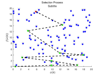
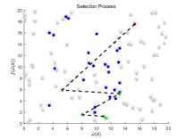
To illustrate the utility of the above proposed algorithm, an example simulation about 100 distinct random points will be given. In detail, their horizontal and vertical coordinates referred to be and respectively are randomly generated on interval , which are further denoted as and . First of all, some simulations are shown in Fig. 1, in which different search radius such as , , and are given.
 |
 |
 |
 |
| : = 20 | : = 10.71 | : = 5.68 | : = 2.84 |
 |
 |
 |
 |
| : = 20 | : = 10.71 | : = 5.68 | : = 2.84 |
On the one hand, the red point is the initial iteration point, and the gray points are “useless” ones which are not used at all. Without loss of generality, two situations about different initial iteration points such as Point 16 and Point 83 are considered. Their horizontal and vertical coordinates are selected to be and respectively. On the other hand, the blue points are the failed ones during the iteration, while the green ones are the successful ones satisfying the update law (16). By investigating these simulations, it can be found that the bigger the value takes, the smaller the value arrives. However, the computation complexity will be larger as takes bigger values. To the contrary, when the radius is selected to be small enough, it can be concluded from Fig. 1 that the computation complexity will be great reduced. However, the probability of the obtained optimal solution being a locally optimal solution will be higher and have a worse quality. Thus, how to select a suitable radius is also one topic studied in this paper.
The search radius of (14) is selected to be
| (17) |
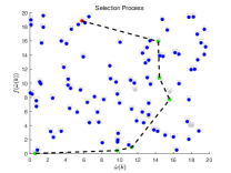
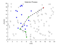
where is a attenuation coefficient. Particularly, the initial search radius is also defined as , where is given to be
Then, one can get a simulation Fig. 2 similar to Fig. 1, where the values of about the initial radius are selected to be , , and respectively. Accordingly, the values of initial radius about initial value based on (17) are computed to be , , and respectively. Meanwhile, the values of initial radius about initial value are computed to be , , and respectively. On the one hand, by the simulations of Fig. 2 presented in rows respectively, it can be concluded that the computation complexity is usually reduced along with decreasing under the same initial condition. On the other hand, in order to make some comparisons between Fig. 1 based on (14) and Fig. 2 based on (17), it had better to compare them under the same conditions such as the same and . Thus, only a part but not all the subgraphs are necessary to make comparisons such as the comparisons on subgraphs , , and , between Fig. 1 and Fig. 2 respectively. In detail, not only the fewer iteration times but also the fewer failed points are presented in Fig. 2. More importantly, the convergence of nominal solution is guaranteed in Fig. 2, which is not satisfied in Fig. 1. However, there is also a negative effect that the gaps among the locally optimal solutions obtained in Fig. 2 are bigger, some of which are farther away from the globally optimal solution to subgraphs and of Fig. 1. Thus, it is necessary to further study the effect of variable radius in order to give an optimal variation of radius .
 |
 |
 |
 |
 |
 |
 |
 |
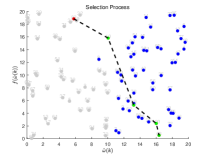
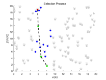
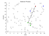
For another, based on (17), it can be known that plays an important role in generating variable . In order to realize an optimization to radius , expression (17) is revised to be
| (18) |
where . Similar to the definition in (17), it is defined as . Then, similar to Fig. 2, similar simulations under (18) are given in Fig. 3. Particularly, the initial values of parameters and of subgraphs in Fig. 3 are given such as ; ; ; ; ; ; and . By making the comparisons of all the subgraphs between Figs. 2 and 3, it can be found that less computation complexity of (18) is presented in Fig. 3, whose iteration time is fewer too. Moreover, the minimum value of obtained in Fig. 2 based on (17) is larger than one in Fig. 3 by applying (18). In other words, it is necessary and important to study how to select the detailed value during every iteration to gain a better performance such as smaller value of (12), less computation complexity, but better monotonicity and convergence. All these problems will be considered and finally solved in this paper.
 |
 |
 |
 |
 |
 |
 |
 |
Definition 1
A control update sequence is said to have the finite sampling rate property if there exists a scalar such that , .
Assumption 1
It is assumed that the event-triggered sampling interval , , has an upper bound such as , where , , and , , .
III Main results
Theorem 1
Consider the system composed of (1) and (3), where the detailed classification of controller (3) is assumed to be given in advance such that is given beforehand, so do the and , , . Then, the related closed-loop system is GAS a.s., if given parameters , and , there exists a matrix satisfying
| (19) |
| (20) |
| (21) |
where , , and , , is the stationary distribution of the embedded chain of semi-Markov process. Meanwhile, the upper sampling bound is computed by
| (22) |
where and .
Proof The proof is given in Appendix A.
Next, Problems 1 and 2 will be considered. Before discussing them, a convex optimization problem with some constraints should be proposed first. On the one hand, from Example 3.11 of [27] on Page 82, it is clear that , but given , is convex. Moreover, function is also convex. On the other hand, even if the set classification of controllers is fixed, the given conditions of Theorem 1 to be as constraints will be hard to be solved in the optimization problems, since parameters and are vector and matrix variables respectively. As a result, different from Theorem 1, not only satisfying but also here is given beforehand. Without loss of generality, they will be calculated by following LMIs
| (23) |
| (24) |
and (21), where , and are given scalars, and and are variables to be computed by solving the above LMIs. Due to page limitation, the detailed calculation process is omitted here.
Remark 2
It is worth mentioning that the computation way for and described in (21), (23) and (24) is not unique. In other words, they can be computed in advance by other ways, as long as the corresponding conditions described by (19)-(21) with given and satisfy. Naturally, there exist inevitable differences among the different techniques providing different parameters’ values. However, such differences will not lead to essential distinctions to the optimization problems in this paper and will not discuss in detail.
Since the parameters of Theorem 1 such as , , , and are given beforehand, conditions (20) and (21) are known and always satisfied. In detail, parameters , , and are defined by (21), (23) and (24), while is a new given parameter and only defined in (19). Then, the constraints described by conditions (19)-(21) are equivalently simplified to be
| (25) |
where
According to Example 2.10 on Page 38 and Example 3.11 on Page 82 of [27], it is clear that constraint (25) is a convex set. Then, a convex optimization problem described by cost function (11) with constraint (25) is successfully proposed. According to Example 3.10 of [27] on Page 82, it can be concluded that function is also convex. Thus, the feasible domain of (25) is equivalently rewritten to be
| (26) |
Since (26) being inequalities, a slack variable such as is introduced to change (26) be an equation constraint such as
| (27) |
Based on the given results of [28] on Pages 98 and 99, it can be known that such slack variables do not bring any negative effects to (26) but make the equivalent constraint (27) solved easily. Moreover, it can be concluded that constraint (27) is convex. Thus, the original convex optimization problem is transformed into convex cost function (11) with convex constraint (27). In order to solve this convex optimization problem, an augmented Lagrangian function is constructed as
| (28) | ||||
where
and penalty factor . Here, is the slack variable and is the multiplier. Because (11) and (27) are both convex, it is obvious that function (28) is convex too.
Meanwhile, it is obvious that the above computation process of the globally optimal value should be repeated by selecting every . Based on the above illustrations and simulations about mode classification, the repetition number of computation will equal to the Stirling number of the second kind. Obviously, the computation complexity will be very large especially and increase big. In order to deal with this problem and motivated by the phenomena discovered in Figs. 1-3, an optimization algorithm based on an improved HCA will be developed, which can generate an iteration sequence of solution and so does the corresponding sequence of objective function . Moreover, the locally optimal solution and its value can be reached such as . Moreover, one can conclude from Figs. 1-3 that strategy (18) will be the best if its dynamically attenuation coefficient is suitably adjusted. In detail, it not only ensures all the advantages of strategy (17) but also improves the iteration speed and the quality of optimal solution . How to dynamically adjust the attenuation coefficient to make (18) work optimally is an open problem. Here, we will use the Q-learning algorithm to dynamically adjust , so as to dynamically change the radius of search interval and lead to an improvement in performance. Meanwhile, it is very necessary and important to analyze its mathematical model, which includes the state, action, and reward function.
State: The state is a feedback of the agent at the th step and denotes the impact of its taking action on the environment. Here, described as the produced solution at step such as . Meanwhile, a termination state should be given beforehand but does not belong to the solution set . Its aim is to end the current training round when the state arrives at the termination state . Finally, the state space is composed of the solution set of HCA and the termination state such as .
Action: The action is a description of the agent’s behavior at the th step. Here, it is the specific value of of HCA at the th iteration step such as , which can change the neighborhood set and affect the generation of the next solution. As a result, all values of or constitute the action space .
Reward: The reward is a feedback of the environment in which the agent has taken the action in state . Here, it is described by
| (29) |
where function has been defined in (13). In detail, two situations will be found if condition is satisfied. On the one hand, the agent will be penalized and receive a negative reward, if the agent takes an action in state such that the solution satisfies . On the other hand, the agent will be encouraged and receive a positive reward, if the solution satisfies . In other words, if the agent wants to obtain a larger positive reward, the solution should satisfy not only is larger than as much as possible, but also the distance between and is as small as possible. To the contrary, means the neighbor set of is the empty set. It also means that no solution within whose objective function value is smaller than . In this situation, the agent is still penalized but receives a negative reward . Then, according to [29] on Page 70, it is well known that the Q-learning effect of taking action in state can be depicted by the Q-value, i.e. it can make an evaluation about the variation of . Accordingly, a specific definition of Q-value similar to (3.11) in [29] is given as
| (30) |
where is the Q-value and quantizes the effect of taking action followed by the policy in state , and is a given discount factor. Particularly, policy is a mapping from each state and action to the probability of taking action when in state . As a result, a different taking action can be generated by a different strategy in state and will lead to a different . In detail, when the Q-value is larger, the taking action will be better. To the contrary, the action selection will be worse.
Theorem 2
Consider a convex optimization problem described by (11) and (25), where the parameters and are computed by solving conditions (21), (23) and (24), and parameters , , and are also given in advance. The optimization problem (11) constrained on (25) will have a globally optimal solution, if the following conditions are satisfied
| (31) |
| (32) |
| (33) |
Then, the globally optimal value of (11) is obtained by
| (34) |
Meanwhile, the globally optimal solution is computed by
| (35) |
Particularly, in order to get an optimal solution to convex problem (11) with (25) without computing one by one, an improved HCA based on Q-learning (Q-HCA) is proposed, whose searching radius iteration rule is given in (18). Meanwhile, is obtained by the Q-learning with state , action and reward presented in (29). Then, an iteration rule for estimating Q-value (30) is given as
| (36) |
where is the given learning rate, and is the set of taking actions in state . As a result, an optimal attenuation coefficient is obtained. Moreover, under any initial condition with similarly defined in (17), a preferably nominal solution sequence with can be developed by following rules (36) and (18), where is a maximum value of iteration. Thus, a locally optimal solution to convex problem (11) with (25) satisfying a part of is computed by
| (37) |
Meanwhile, the corresponding value of (11) is also locally optimal such as and described to be
| (38) |
More importantly, both convergence and monotonicity properties of Q-HCA are ensured. Finally, the upper sampling bound of the related optimal controllers is also computed by (22).
Proof The proof is given in Appendix B.
Specially, when controller (3) has no sampling phenomenon, it will reduce to be
| (39) |
where and are similar to (3), and function also has the similar definition but on interval . Then, one has the following corollaries.
Corollary 1
Proof The proof is established by Theorem 1 and omitted.
Remark 3
When parameter of controller (39) is selected to be special values such as , if ; , otherwise. Accordingly, controller (39) can be simply rewritten as and similar to [17] which is related to the stationary distribution probability. In this situation, similar results can be obtained and omitted for page limitation. Particularly, if all the values of are equal such as , and , a mode-independent controller with will be obtained and similar to [17, 22]. In other words, Corollary 1 contains some existing results as special situations, which is more general and less conservative.
Accordingly, when the mode classification is not given in advance and similar to (10), controller (39) is described as
| (42) |
After giving parameters and , one can compute and by solving conditions (21), (24) and
| (43) |
Then, similar to constraint (25), the constraint of the above conditions is equivalently simplified to be
| (44) |
where
A similar augmented Lagrangian function is constructed as
| (45) | ||||
where
and parameers and are defined in (28). Then, one can obtain the following corollary.
Corollary 2
Consider a convex optimization problem described by (11) and (44), where the parameters and are computed by solving conditions (21), (24) and (43) under giving parameters and . The optimization problem (11) constrained on (44) will have a globally optimal solution, if the following conditions are satisfied
| (46) |
| (47) |
| (48) |
Then, the globally optimal value of (11) is obtained by
| (49) |
Meanwhile, the globally optimal solution is computed by
| (50) |
Moreover, based on the developed Q-HCA algorithm, one also gets a locally optimal solution and its locally optimal value such as (37) and (38) without computing one by one.
Proof Its proof is similar to Theorem 2 and omitted.
Remark 4
It can be seen that some parameters such as and in main results need to be given in advance. Particularly, in order to give them easily and directly, they are solved by some LMIs such as (23) and (24). It is worth noted that these convenient techniques will lead to some conservatism in terms of some of constraints such as (25) unsatisfied. In this situation, some possible ways may be used to deal with them, and only two possible ways are mentioned here. On the one hand, one can select different values of the scalars given in the presented LMIs time and time again, until the dissatisfied constraints hold. On the other hand, other different conditions providing and in advance can be developed so as to make the dissatisfied constraints satisfying.
IV Numerical example
Example 1: Considering a system of form (1) with whose matrices are described as
The transition probabilities of the embodied chain is given as
It has a unique stationary distribution computed as . In addition, the expectations of sojourn time for modes are given to be , , , and . Firstly, based on conditions (23) and (24), after letting , , , , , , , , , and , one can obtain that , and the control gains are computed such as , , , and , while matrix is computed as
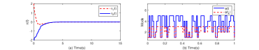
As we know, based on the commonly mode-dependent methods, see, e.g., [1, 2, 3, 4, 6], there will be 5 controllers since the mode quantity of this example is 5. More importantly, an ideal assumption that the switching signals between controller and other system matrices should be synchronous is also needed. To the contrary, the method in this paper can provide fewer effective controllers whose modes are not necessary synchronous to system matrices’, which has larger application scope. Without loss of generality, set is separated into 3 classes such as . Consequently, it can be computed that with and , and the classification parameter is the same to Table I. Then, after applying the above designed controllers in addition to some related parameters, the optimal value with its optimal solution of each classification is given in Table II, where is denoted as the ultimate upper sampling bound. It can be seen from this table that there is no optimal solution to some classifications. The reason is that the given parameters and computed by (23) and (24) dissatisfy constraint (25), whose possibly solvable algorithms are presented in Remark 4. Moreover, some comparisons between this paper and some similar existing references can be done in the next. In references [19, 18, 20], a method based on an auxiliary system approach was found and can be used to discuss stochastic systems having a sampling phenomenon in either state or switching or both of them. Since their methods about sampling are the same, without loss of generality, only comparisons between this paper and [18] are enough. Under the above given parameters and by using the method in [18], the maximum sampling upper bound can be computed as . It is far less than which results from the globally optimal solution such as , , , , and and also corresponds to the situation of Table II with . It can be further seen from Table II, all the upper sampling bounds are larger than , so long as there exists a suitable solution. Based on these comparisons, it can be concluded that the developed mode classification and optimization method is superior to the above auxiliary system approach for providing a larger sampling interval and improving the efficiency of communication network. Moreover, under the initial condition and selecting any effective classification such as , , , corresponding to in Table II, one can compute its controller such as , and . Then, the state curves of the closed-loop system are shown in Fig. 4 (a), and the schematic diagram of mode signals is displayed in Fig. 4 (b). Although both state and mode are sampled, the presented controller is still useful in stabilizing a stochastic system.
| 1 | 0.46 | 0.47 | -0.07 | 1.66 | -0.69 | 3.3820 | 0.0174 |
|---|---|---|---|---|---|---|---|
| 2 | – | – | – | – | – | – | – |
| 3 | 0.46 | 2.70 | 0.05 | 0.24 | -0.12 | 3.5891 | 0.0146 |
| 4 | 0.46 | 1.50 | -0.18 | 0.57 | 0.45 | 4.5422 | 0.0142 |
| 5 | – | – | – | – | – | – | – |
| 6 | 0 | 11.83 | -1.70 | 0.24 | 0.45 | 4.8947 | 0.0136 |
| 7 | 0.68 | 0.47 | -0.09 | 1.23 | 0.45 | 6.4733 | 0.0123 |
| 8 | – | – | – | – | – | – | – |
| 9 | – | – | – | – | – | – | – |
| 10 | 0 | 11.83 | -1.70 | 0.24 | 0.45 | 4.8947 | 0.0137 |
| 11 | 0.46 | 16.92 | -2.65 | -0.80 | 1.09 | 4.5637 | 0.0146 |
| 12 | 0.46 | -4.97 | 1.08 | 1.68 | -0.82 | 3.7408 | 0.0172 |
| 13 | 0.46 | -0.51 | 0.10 | 0.75 | 0.57 | 5.1091 | 0.0153 |
| 14 | -1.88 | 0.47 | 0.99 | -0.80 | 1.09 | 9.2897 | 0.0123 |
| 15 | 0 | 0.47 | 0.67 | 0.24 | -0.18 | 3.9675 | 0.0174 |
| 16 | 0 | 0.47 | -0.08 | 1.01 | 0.45 | 4.9755 | 0.0161 |
| 17 | – | – | – | – | – | – | – |
| 18 | – | – | – | – | – | – | – |
| 19 | – | – | – | – | – | – | – |
| 20 | 0.40 | 0.08 | 0.67 | 0.24 | -0.18 | 4.0838 | 0.0173 |
| 21 | -1.88 | -4.01 | 0.99 | 0.24 | 1.39 | 9.4961 | 0.0123 |
| 22 | 0 | 16.92 | -2.65 | 0.24 | 0.45 | 4.8516 | 0.0146 |
| 23 | 0 | 0.59 | -0.10 | 1.06 | 0.45 | 5.0880 | 0.0174 |
| 24 | -1.88 | -1.43 | 0.99 | 0.65 | 0.45 | 9.6922 | 0.0091 |
| 25 | 0 | 16.92 | -2.65 | 0.26 | 0.45 | 4.8516 | 0.0146 |
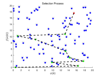
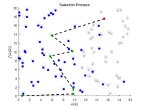
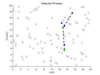
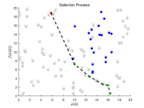
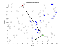
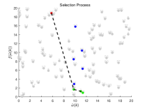
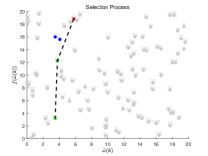
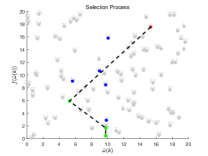
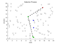
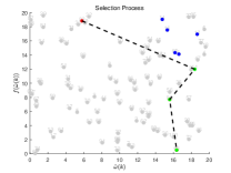
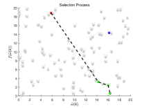
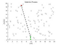
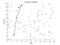
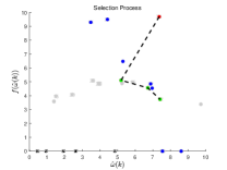
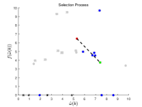
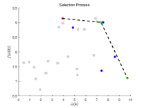
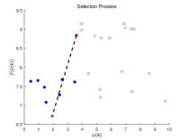
Furthermore, based on the developed Q-HCA in Theorem 2, a suboptimal solution or even an optimal solution can be obtained. In detailed, the iteration processes under different initial points are shown in Fig. 5 with , where the points in the horizontal axis denote as infeasible points. Particularly, the infeasible points in blue means that they have been selected to participate in calculation, while the black ones are only infeasible points but without being selected during the iteration. Moreover, from this simulation, it can be seen that when the initial points are Points 24 and 7 respectively, the final point is Point 12 corresponding to in Table II, whose cost function is computed as . Similarly, one can further know that when the initial point is Point 14, the final point is Point 3 with . And when the initial point is Point 7, the final point is Point 1. Especially, in this situation, its cost function is computed as and equals to the globally optimal value . Obviously, by comparing Table II and Fig. 5, one can obtain that the computation complexity and time of Fig. 5 by the Q-HCA method is both largely reduced and without computing mode classification one by one. Moreover, it also can be seen from Fig. 5 that the convergence of the Q-HCA method is also ensured, which is asymptotically convergent. In a word, all the statements about the effectiveness and superiority of the developed method in this paper have been shown by the simulations and comparisons.
 |
 |
 |
 |
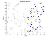
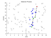
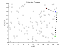
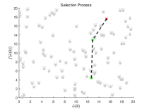
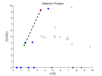
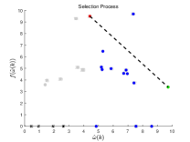
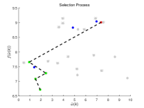
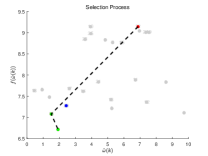
Next, some simulations and comparison about Corollary 2 will be done, where set is also separated into 3 classes such as . First, letting , , , , , , , , and , it can be known from Corollary 2 that . Meanwhile, the control gains computed by conditions (24) and (43) are listed as follows: , , , and . Now, more comparisons will be done. In reference [17], a quantity-limited controller was proposed based on mode separation. However, the optimization problem about such mode separation was not considered in the reference. Moreover, it has been shown there that the method in [17] is less conservative than mode-independent ones [7, 8, 9, 10]. In this situation, only comparisons between Corollary 2 and [17] will be done. Based on [17], it is assumed that modes and are known, and the rest modes are unknown. In this situation, the above assumption is the same as the following mode classification such as , and . Then, by using the method in [17], one can obtain the control gains as , and , and the same cost function (11) about the above designed controllers of [17] is equal to . Investigating all the optimal function value computed similar to Table II and omitted due to page limiation, it can be seen that the global cost function value after optimization is much smaller and less conservative. In order to further illustrate the superiority, more comparisons are done such that a positive perturbation is only added in block (1,1) of matrix such as , and the others remain unchanged. Then, the respective maximum allowable bound about Corollary 2 and [17] under the same is given in Table III, which is denoted as . It is obvious that Corollary 2 by optimizing the mode classifications is less conservative than [17]. Similar to Fig. 5, some simulations about Q-HCA of Corollary 2 under different initial points are given in Fig. 6 with . It can be found that when the initial points are Points 21, 22 and 23 respectively, the final point is Point 2 corresponding to similar to Table II, whose cost function is computed as and equals to the globally optimal value . Also, when the initial point is Point 10, the final point is Point 1 with which is a locally optimal value. As a result, similar conclusions about the given Q-HCA in this paper can be obtained and omitted here.
| -0.1 | -0.2 | -0.3 | -0.4 | -0.5 | |
| 5.595 | 5.562 | 5.529 | 5.496 | 5.463 | |
| [17] | 4.341 | 4.302 | 4.263 | 4.224 | 4.185 |
| -0.6 | -0.7 | -0.8 | -0.9 | -1 | |
| 5.430 | 5.397 | 5.364 | 5.331 | 5.298 | |
| 4.146 | 4.108 | 4.069 | 4.030 | 3.991 |
 |
 |
 |
 |
Finally, more comparisons will be done to further demonstrate the advantages of the method proposed here. As we know, a sampled system can be discussed by transforming the sampled term into a time-varying delay term. Similarly, when both state and switching are sampled, a input delay approach was used in [33]. Unfortunately, its method has some limits such that it cannot be used to stabilize an MJS having non-negative eigenvalues. Meanwhile, an augmented system approach was presented in [21] and can be used to deal with MJSs with sampled state and switching simultaneously. Due to it considering about MJSs instead of semi-Markovian jump systems (SMJSs) and in order to make some comparisons, it is assumed that the related system in this example is reduced to be an MJS. In detail, all the system parameters are the same as the above SMJS, except the transition rate matrix of MJSs is given as
Then, based on [21] with given control gains such as , , , and , one can get the upper sampling bound is . On the other hand, it can be known that similar results about MJSs can be easily obtained from the results about SMJSs. Thus, under the same control gains given above, and selecting , , , and with a specific mode classification such as , and , the upper sampling bound based on Theorem 1 without any optimization is equal to . It showns that the method in this paper can provide a larger sampling bound and is less conservative than [21].
V Conclusions
In this study, the sampled stabilization for stochastic jump systems has been investigated by a mode classification optimization method. A new mode-classification-based controller has been proposed to handle the general sampling situation that both controller’s state and switching are sampled. So as to find the best classification for stabilization, an optimization problem has been proposed to provide a globally optimal solution among such classifications. An Q-HCA algorithm has been established to provide an optimal attenuation coefficient, whose monotonicity and convergency have been both satisfied. Finally, the utility and advantage of this paper have been obviously illustrated and shown by a numerical example.
References
- [1] H. Zhang, J. Wang, Z. Wang and H. Liang, “Mode-dependent stochastic synchronization for Markovian coupled neural networks with time-varying mode-delays,” IEEE Transactions on Neural Networks and Learning Systems, vol. 26, no. 11, pp. 2621-2634, 2015.
- [2] G. Zhuang, Q. Ma, B. Zhang, S. Xu and J. Xia, “Admissibility and stabilization of stochastic singular Markovian jump systems with time delays,” Systems and Control Letters, vol. 114, pp.1-10, 2018.
- [3] B. Cai, L. Zhang and Y. Shi, “Observed-mode-dependent state estimation of hidden semi-Markov jump linear systems,” IEEE Transactions on Automatic Control, vol. 65, no. 1, pp. 442-449, 2019.
- [4] K. Ding and Q. Zhu, “Extended dissipative anti-disturbance control for delayed switched singular semi-Markovian jump systems with multi-disturbance via disturbance observer,” Automatica, vol. 128, pp. 109556, 2021.
- [5] W. Qi, Y. Zhou, L. Zhang, J. Cao and J. Cheng, “Non-fragile SMC for Markovian jump systems in a finite-time,” Journal of the Franklin Institute, vol. 358, no. 9, pp. 4721-4740, 2021.
- [6] R. Zhang, H. Wang, J. H. Park, K. Shi and P. He, “Mode-dependent adaptive event-triggered control for stabilization of Markovian memristor-based reaction-diffusion neural networks,” IEEE Transactions on Neural Networks and Learning Systems, vol. 34, no. 8, pp. 3939-3951, 2023.
- [7] C. E. de. Souza, A. Trofino and K. A. Barbosa, “Mode-independent filters for Markovian jump linear systems,” IEEE Transactions on Automatic Control, vol. 51, no. 11, pp. 1837-1841, 2006.
- [8] H. N. Wu, and K. Y. Cai, “Mode-independent robust stabilization for uncertain Markovian jump nonlinear systems via fuzzy control,” IEEE Transactions on Systems Man and Cybernetics Part B-Cybernetics, vol. 36, no. 3, pp. 509-519, 2005.
- [9] P. H. Liu, D. W. C. Ho and F. C. Sun, “Design of filter for Markov jumping linear systems with non-accessible mode information,” Automatica, vol. 44, no, 10, pp. 2655-2660, 2008.
- [10] X. Li, W. Zhang and D. Lu, “Robust asynchronous output-feedback controller design for Markovian jump systems with output quantization,” IEEE Transactions on Systems, Man, and Cybernetics: Systems, vol. 52, no. 2, pp. 1214-1223, 2022.
- [11] G. L. Wang, B. Y. Li, Q. L. Zhang and C. Y. Yang, “A partially delay-dependent and disordered controller design for discrete-time delayed systems,” Interational Journal of Robust Nonlinear Control, vol. 27, no. 16, pp. 2646-2668, 2017.
- [12] O. L. V. Costa, M. D. Fragoso and M. G. Todorov, “A detector-based approach for the control of Markov jump linear systems with partial information,” IEEE Transactions on Automatic Control, vol. 60, no. 5, pp. 1219-1234, 2014.
- [13] G. L. Wang, Q. L. Zhang and C. Y. Yang, “Fault-tolerant control of Markovian jump systems via a partially mode-available but unmatched controller,” Journal of the Franklin Institute, vol. 354, no. 17, pp. 7717-7731, 2017.
- [14] G. L. Wang and L. Xu, “Almost sure stability and stabilization of Markovian jump systems with stochastic switching,” IEEE Transactions on Automatic Control, vol. 67, no. 3, pp. 1529-1536, 2022.
- [15] G. L. Wang and Y. Y. Sun, “Almost sure stabilization of continuous-time jump linear systems via a stochastic scheduled controller,” IEEE Transactions on Cybernetics, vol. 52, no. 5, pp. 2712-2724, 2022.
- [16] G. L. Wang, Y. S. Ren and Z. Q. Li, “Almost Sure Stabilization of Continuous-Time Semi-Markov Jump Systems via an Earliest Deadline First Scheduling Controller,” IEEE Transactions on Systems, Man, and Cybernetics: Systems, vol. 54, no. 1, pp. 656-667, 2024.
- [17] G. L. Wang, “Stabilization of semi-Markovian jump systems via a quantity limited controller,” Nonlinear Analysis: Hybrid Systems, vol. 42, Artical: 101085, 2021.
- [18] X. Mao, “Stabilization of continuous-time hybrid stochastic differential equations by discrete-time feedback control,” Automatica, vol. 49, no. 12, pp. 3677-3681, 2013.
- [19] X. Mao, “Almost sure exponential stabilization by discrete-time stochastic feedback control,” IEEE Transactions on Automatic Control, vol. 61, pp. 1619-1624, 2015.
- [20] G. F. Song, Z. Y. Lu, B. C. Zheng and et al, “Almost sure stabilization of hybrid systems by feedback control based on discrete-time observations of mode and state,” Science China Information Sciences, vol. 61, pp. 70213, 2018.
- [21] G. L. Wang, Y. S. Ren and C. Huang, “Stabilizing control of Markovian jump systems with sampled switching and state signals and applications,” Interational Journal of Robust Nonlinear Control, vol. 33, no. 10, pp. 5198-5228, 2023.
- [22] G. L. Wang, “Mode-independent control of singular Markovian jump systems: A stochastic optimization viewpoint,” Applied Mathematics and Computation, vol. 286, pp. 155-170, 2016.
- [23] B. C. Rennie and A. J. Dobson, “On stirling numbers of the second kind,” Journal of Combinatorial Theory, vol. 7, no. 2, pp. 116-121, 1969.
- [24] K. N. Boyadzhiev, “Close encounters with the Stirling numbers of the second kind,” Mathematics Magazine, vol. 85, no. 4, pp. 252-266, 2012.
- [25] S. H. Jacobson and E. Ycesan, “Analyzing the performance of generalized hill climbing algorithms,” Journal of Heuristics, vol. 10, pp. 387-405, 2004.
- [26] X. T. Wu, Y. Tang, J. D. Cao and X. R. Mao, “Stability analysis for continuous-time switched systems with stochastic switching signals,” IEEE Transactions on Automatic Control, vol. 63, no. 9, pp. 3083-3090, 2017.
- [27] S. P. Boyd and L. Vandenberghe, Convex optimization. Cambridge university press, 2004.
- [28] F. S. Hillier, Introduction to operations research. McGrawHill, 2001.
- [29] R. S. Sutton and A. G. Barto, Reinforcement learning: An introduction. MIT press, 2018.
- [30] Y. J. Wang and Z. A. Liang, Optimization of the basic theory and methods. Fudan University Press, 2011.
- [31] D. P. Bertsekas, Constrained optimization and Lagrange multiplier methods. Academic press, 2014.
- [32] C. J. C. H. Watkins and P. Dayan, “Q-learning,” Machine learning, vol. 8, pp. 279-292, 1992.
- [33] G. L. Wang and Y. S. Ren, “Stability analysis of delayed Markovian jump systems with delay switching and state signals and applications,” Interational Journal of Robust Nonlinear Control, vol. 32, no. 9, pp. 5141-5163, 2022.
VI Appendix
VI-A Proof of Theorem 1
First of all, , , is defined to be the switching quantity of on interval . For any , and , one concludes that and . Consequently, one gets and , , from event-triggered mechanism (4) under Assumption 1. Moreover, one can further obtain such that every subinterval of such as or certainly belongs to one subinterval of such as or uniquely. Alternatively, established based on principle (4) is a subsequence of . As a result, and without loss of generality, it is assumed that
| (51) |
where and . Particularly, is denoted as
| (52) | ||||
In addition, for , one can conclude that , if . Then, after applying (3), the system (1) closed by an event-triggered controller described by (3)-(8) is equal to
| (53) |
Accordingly, choose the Lyapunov function as and based on (51)-(53) and condition (20), for any , one gets that
| (54) | ||||
| (55) | ||||
| (56) | ||||
Particularly, the above inequalities holding also need the following condition
| (57) | ||||
where , and . On the other hand, let , , it can be concluded from (53) that
| (58) |
Its solution is computed as
| (59) |
which implies
| (60) | ||||
It can be known that function , , is monotonically increasing with and . Based on Assumption 1, one has
| (61) |
Then, one obtains that
| (62) |
When function satisfies
| (63) |
where is a suitable design parameter, inequality (62) becomes to be
| (64) |
Under condition , inequality (57) is equivalent to
| (65) | ||||
Based on condition (19) and (64), inequality (65) is guaranteed. Thus, conditions (54)-(56) are satisfied. They finally yield that for ,
| (66) | ||||
Then, one could obtain that
| (67) |
It is obvious from (21) that there is always a scalar such that
| (68) |
Then, similar to the proof of Theorem 1 in [26], one knows that if and defined in (68), there exists a positive constant such that if , then
| (69) |
Accordingly, for , one has
| (70) | ||||
Based on the strong law of large numbers, one obtains that
| (71) |
Then, it can be concluded from (21) that
| (72) |
Consequently, one gets that
| (73) |
Based on the above equation, it can be known that for any given scalars and , there exits a random variable such that
| (74) | |||
Then, for any and combing conditions (67) and (74), one can conclude condition . Moreover, it can be concluded from (74) that
| (75) |
Obviously, for any , there is always such that
| (76) |
By selecting and letting , and considering inequality (67) under condition (76), one has
| (77) | ||||
which implies condition . Due to conditions and both satisfying, the resulting closed-loop system is finally GAS a.s..
VI-B Proof of Theorem 2
On the one hand, first of all, it is obvious that the augmented Lagrangian function (28) is convex. Then, based on the result given in [30] on Page 108, it can be concluded that there exists a globally optimal solution to (28) which can be computed by solving conditions (31)-(33) and defined as . Particularly, it can be seen that (28) is strictly convex about such as . In other words, there is only one globally optimal solution satisfying (31)-(33). Meanwhile, according to reference [31] on Page 97, it can be known that the optimization problem (11) constrained by (27) has the same optimal value as the optimization problem (28). That is
| (81) |
Finally, one can easily obtain the globally optimal value of (11) with constraint (27) described by (34), whose corresponding optimal solution is obviously computed by (35).
On the other hand, it has been shown in [32] that generated by (36) can theoretically converge to with probability 1 when . As a result, an optimal taking action , , maximizing Q-value (30) can be established, which is actually an optimal attenuation coefficient . Then, a preferable searching radius , , can be gotten based on the iterative update rule (18), while the initial condition is given to be but should be given such as one defined in (17). Based on the obtained , a preferably nominal solution referred as , , can be gotten by using HCA. Finally, by repeating the above process along with iteration number having a maximum value , two optimal sequences and can be established based on (36), while two preferable sequence and with can also be developed by (18). The detailed repeating process is given as follows:
Consequently, based on the characteristics of Q-HCA, it can be obviously known that sequence will have a good convergence characteristic such as (37). Meanwhile, the monotonicity of (38) can be guaranteed. Moreover, since all the elements of belong to but is only a part of , it is obviously concluded that the obtained optimal value will be no less than obtained by (34). In this situation, it can be said that the above obtained is only a locally optimal solution. Finally, the iteration process of the developed Q-HCA is given below:
| Algorithm 1: Improved hill climbing algorithm based on Q-learning |
| Initial Q-values with Q-HCA, parameter , iterative index = 1, |
| Select a starting state , calculate by the parameter |
| while ( maximum number of iterations) |
| while is not a termination state |
| Choose according to the |
| Take action |
| Return reward by the equation (29) |
| Update Q-value by the equation (36) |
| Update by the equation (19) |
| Update of corresponding to |
| by the equation (14) |
| if is not empty set |
| Generate a new state by of |
| corresponding to |
| Move to new state |
| else if is empty set |
| Move to the termination state |
| end if |
| end while |
| end while |
This completes the proof.