The ghost-gluon vertex in the presence of the Gribov horizon: general kinematics

Abstract

Correlation functions are important probes for the behavior of quantum field theories. Already at tree-level, the Refined Gribov Zwanziger (RGZ) effective action for Yang-Mills theories provides a good approximation for the gluon propagator, as compared to that calculated by nonperturbative methods such as Lattice Field Theory and Dyson-Schwinger Equations. However, the study of higher correlation functions of the RGZ theory is still at its beginning. In this work we evaluate the ghost-antighost-gluon vertex function in Landau gauge at one-loop level, in $d=4$ space-time dimensions for the gauge groups SU(2) and SU(3). More precisely, we extend the analysis conducted in Mintz et al. (2018) for the soft-gluon limit to an arbitrary kinematic configuration. We introduce renormalization group effects by means of a toy model for the running coupling and investigate the impact of such a model in the ultraviolet tails of our results. We find that RGZ results match fairly closely those from lattice simulations, Schwinger-Dyson equations and the Curci-Ferrari model for three different kinematic configurations. This is compatible with RGZ being a feasible theory for the strong interaction in the infrared regime.

I Introduction

Since the proposal of Quantum Chromodynamics (QCD) as the theory of Strong Interactions, a long path was constructed to connect the fundamental degrees of freedom – quarks and gluons – to the observed physical states and processes. At high energies, asymptotic freedom allows for a perturbative approach that, supplemented by essential nonperturbative information in Particle Distribution Functions and fragmentation phenomena, agrees with a plethora of experimental output from high-energy particle colliders. The infrared (IR) regime however is much less amenable. Monte Carlo simulations that solve the Euclidean version of QCD on a discretized space-time lattice have by now and with great effort established that this non-Abelian theory can quantitatively describe several hadronic observables Fodor and Hoelbling (2012); Durr et al. (2008); Borsanyi et al. (2021, 2015). Nevertheless, the mechanism of color confinement is still an open question, calling for the development of continuum approaches and (semi)analytical descriptions of the infrared behavior of Strong Interactions. Among the well-developed continuum methods that try to tackle this non-perturbative regime, Schwinger-Dyson equations Bashir et al. (2012); Aguilar et al. (2016, 2023, 2022, 2021a, 2021b); Huber et al. (2021); Aguilar et al. (2021a); Fischer and Huber (2020); Huber (2020); Aguilar et al. (2019) stand out in different hadronic applications, but also the Functional Renormalization Group Berges et al. (2002); Pawlowski (2007); Corell et al. (2018); Cyrol et al. (2016); Fischer et al. (2009); Dupuis et al. (2021) and effective models Nambu and Jona-Lasinio (1961); Klevansky (1992); Gell-Mann and Levy (1960); Fukushima (2004); Schaefer et al. (2007) have been employed with partial success. Other approaches, such as the Curci-Ferrari (CF) model in Landau gauge Tissier and Wschebor (2010, 2011); Pelaez et al. (2013); Peláez et al. (2014, 2015); Gracey et al. (2019); Peláez et al. (2021); Figueroa and Peláez (2022); Barrios et al. (2020, 2021, 2022) and the screened massive expansion Siringo (2023); Siringo and Comitini (2023); Comitini et al. (2021); Comitini and Siringo (2020); Siringo and Comitini (2018) have successfully described some aspects of the IR of Yang-Mills theory by employing perturbation theory.

Here we adopt another continuum approach to the nonperturbative regime of Yang-Mills theories: the Refined Gribov-Zwanziger (RGZ) theory Dudal et al. (2008, 2010). This framework, as the other continuum methods, adopts a gauge-fixed setup and is formulated from first-principles as a gauge path integral modified in the infrared by the existence of Gribov gauge copies. This idea follows the seminal work by Gribov himself Gribov (1978) and the development of local actions attained by Zwanziger Zwanziger (1989) and complemented by the emergence of dimension two condensates Dudal et al. (2008, 2010, 2019). For comprehensive reviews, the reader is referred to Vandersickel and Zwanziger (2012); Vandersickel (2011); Sobreiro and Sorella (2005) and references therein.

The presence of this nonperturbative background stemming from the Gribov horizon and the condensates seems to carry plenty of information from the interacting theory, so that the remaining interaction corrections might be supposed to be small, i.e. perturbative. Even at tree-level, the RGZ gluon propagator is compatible with the deep IR behavior observed on Landau-gauge Lattice QCD data Dudal et al. (2008), while reducing to pure Yang-Mills at large energies Capri et al. (2016a) in a fully self-consistent formulation that would include solving the Gribov gap equation and the effective potential for the different condensates. Gauge-parameter independence of gauge-invariant quantities in this setup is under control within linear covariant gauges through a nilpotent Becchi-Rouet-Stora–Tyutin symmetry, and the predictions for the gluon propagator in general covariant gauges are also compatible with available lattice results Capri et al. (2015, 2016b, 2016c, 2017).

In this paper, the aim is to take a step forward in the direction of establishing predictions of the RGZ theory by including radiative corrections and confronting them with lattice data and other nonperturbative approaches. This is crucial for further understanding whether this theory can be a consistent model of infrared Yang-Mills and eventually QCD. Previous results on the vertices of the (R)GZ action in the Landau gauge may be found in Ref. Gracey (2012). Here, in particular, we compute the general kinematics of the gluon-ghost-antighost vertex at one loop order within the RGZ framework, extending previous work on the soft gluon limit of the same correlation function Mintz et al. (2018). The present study enables the investigation of the role played by auxiliary fields in quantitative results in RGZ. In this specific correlation function, we show that the contribution of auxiliary fields, in the form of new vertices and mixed propagators, represents a smaller effect – less than $10\%$ percent – as compared to that of the presence of nonzero pole masses for the gluon. Moreover, we include running effects via an infrared model, with a freezing coupling constant. Even though this is not self-consistently obtained within RGZ, this may be a reasonable approximation, because of the presence of the massive parameters from the horizon and the condensates. Overall we show that the RGZ results are fully compatible with available lattice data for SU(2) and SU(3), as well as other continuum approaches, such as the infrared-safe Curci-Ferrari model in Landau gauge Pelaez et al. (2013); Barrios et al. (2020) and the Dyson-Schwinger equations Aguilar et al. (2019).

This paper is organized as follows. In Sec. II, the formalism of the refined Gribov-Zwanziger framework is presented. In Sec. III, the ghost-antighost-gluon vertex is defined and its general structure in the RGZ theory is discussed. Our computation of generic momentum configurations of the one-loop ghost-gluon vertex is presented in Sec. IV, including the IR running coupling model adopted. Sec. V collects our results along with the corresponding analysis and comparisons with alternative approaches. In Sec. VI we discuss the potential influence of the IR running coupling model on the ultraviolet (UV) tails of our results. We have included perspectives and final remarks in Section VII.

II The Refined Gribov-Zwanziger action in Landau gauge

The Gribov-Zwanziger theory is a framework for making sense of the gauge fixed Yang-Mills theory in the non-perturbative regime. It grew from Gribov’s observation that gauge fixing in the Landau Gauge fails in the strongly coupled regime Gribov (1978); Zwanziger (1989) (see also Vandersickel (2011); Vandersickel and Zwanziger (2012); Sobreiro and Sorella (2005) for reviews), in the sense that gauge copies still exist after the fixing. These are called Gribov copies and they appear in fact in any covariant gauge. The solution proposed by Gribov was to restrict the integration region of the gauge field path integral to the neighborhood containing the perturbative vacuum and bounded by the field configurations associated with the first Gribov copies, called the Gribov Horizon. In the Landau gauge $\partial_{\mu}A^{a}_{\mu}=0$ the Gribov horizon is defined by the set of fields $A^{a}_{\mu}$ for which the equation ${\cal M}^{ab}(A)\alpha^{b}=0$ has a solution, where

$${\cal M}^{ab}(A)(\bullet)=-\delta^{ab}\partial^{2}(\bullet)+gf^{abc}\partial_{\mu}(A^{c}_{\mu}\bullet).$$ (1)

stands for the Faddeev-Popov operator in the Landau gauge.

Zwanziger Zwanziger (1989) was able to recast Gribov’s construction in the form of an effective theory whose restriction to the Gribov horizon is implemented at the level of the action. The resulting action is known as the nonlocal Gribov-Zwanziger action and defined in the Landau gauge in dimension $D$ by

$$S_{nlGZ}=\int d^{D}x\;\left(\frac{1}{4}F^{a}_{\mu\nu}F^{a}_{\mu\nu}+ib^{a}\partial_{\mu}A^{a}_{\mu}+\bar{c}^{a}{\cal M}(A)^{ab}c^{b}\right)+\gamma^{D}H(A)-\gamma^{D}VD\left(N^{2}-1\right)$$ (2)

where $\gamma$ has dimension of mass, $V$ is the space-time volume (formally infinite) and $H(A)$ is known as the horizon function and given by

$$H(A)=g^{2}\int d^{D}p\int d^{D}q\left[f^{abd}\tilde{A}^{d}_{\mu}(-p)\left({\cal M}^{-1}\right)^{bc}_{pq}f^{cae}\tilde{A}^{e}_{\mu}(q)\right]$$ (3)

The mass scale $\gamma$ is not arbitrary, but fixed by a self consistent equation known as the gap equation, which can be written as a condition on a vacuum condensate. Defining

$$Z(\tilde{\lambda})=\int{\cal D}A{\cal D}b{\cal D}\bar{c}{\cal D}c\;e^{-\int d^{D}x\;\left(\frac{1}{4}F^{a}_{\mu\nu}F^{a}_{\mu\nu}+ib^{a}\partial_{\mu}A^{a}_{\mu}-\bar{c}^{a}{\cal M}(A)^{ab}c^{b}\right)+\tilde{\lambda}H(A)-\tilde{\lambda}VD\left(N^{2}-1\right)}$$ (4)

The gap equation reads

$$\frac{\partial Z(\tilde{\lambda})}{\partial\tilde{\lambda}}\Bigr{\rvert}_{\tilde{\lambda}=\gamma^{D}}=0\Rightarrow\langle H(A)\rangle=VD\left(N^{2}-1\right).$$ (5)

The theory as it is is highly non-local due to explicit expression of $H(A)$. In order to have a workable quantum field theory we need to put the action in a local form. This entails the introduction of new, auxiliary fields. We note that

$$\int{\cal D}\varphi{\cal D}\bar{\varphi}{\cal D}\omega{\cal D}\bar{\omega}\;e^{-\int\,d^{4}x\left(\bar{\varphi}^{ac}_{\mu}{\cal M}(A)^{ab}\varphi^{bc}_{\mu}-\bar{\omega}^{ac}_{\mu}{\cal M}(A)^{ab}\omega^{bc}_{\mu}+ig\gamma^{\frac{D}{2}}\,f^{abc}A^{a}_{\mu}(\varphi_{\mu}^{bc}+\bar{\varphi}^{bc}_{\mu})\right)}\sim e^{-\gamma^{D}\;H(A)}$$ (6)

where the symbol $\sim$ means “up to a prefactor” and $(\varphi,\bar{\varphi})$ are complex bosonic fields and $(\omega,\bar{\omega})$ are fermionic fields. Therefore we obtain the local formulation as

$$Z_{GZ}=\int{\cal D}A{\cal D}\bar{c}{\cal D}c{\cal D}b{\cal D}\bar{\varphi}{\cal D}\varphi{\cal D}\bar{\omega}{\cal D}\omega\;e^{-S_{GZ}}$$ (7)

where

$$S_{GZ}= \int d^{D}x\;\left(\frac{1}{4}F^{a}_{\mu\nu}F^{a}_{\mu\nu}+ib^{a}\partial_{\mu}A^{a}_{\mu}-\bar{c}^{a}{\cal M}(A)^{ab}c^{b}\right)$$

$$+\int\,d^{D}x\left(\bar{\varphi}^{ac}_{\mu}{\cal M}(A)^{ab}\varphi^{bc}_{\mu}-\bar{\omega}^{ac}_{\mu}{\cal M}(A)^{ab}\omega^{bc}_{\mu}\right)$$

$$+\int d^{D}x\left(ig\gamma^{\frac{D}{2}}\,f^{abc}A^{a}_{\mu}(\varphi_{\mu}^{bc}+\bar{\varphi}^{bc}_{\mu})-\gamma^{D}D\left(N^{2}-1\right)\right)$$ (8)

and $\gamma$ is such that it satisfies the gap equation (5), which now reads

$$g\langle\,f^{abc}A^{a}_{\mu}(\varphi_{\mu}^{bc}+\bar{\varphi}^{bc}_{\mu})\rangle=\gamma^{\frac{D}{2}}D\left(N^{2}-1\right)$$ (9)

where translation invariance of the vacuum was used to factor out the volume $\int d^{D}x\langle\,f^{abc}A^{a}_{\mu}(\varphi_{\mu}^{bc}+\bar{\varphi}^{bc}_{\mu})\rangle=V\langle\,f^{abc}A^{a}_{\mu}(\varphi_{\mu}^{bc}+\bar{\varphi}^{bc}_{\mu})\rangle$.

The vacuum defined by the gap equation is unstable and favors the formation of new condensates Dudal et al. (2008) that are related to mass scales of the gauge fields $\langle A^{2}\rangle\sim m^{2}$ and auxiliary fields $\langle\bar{\phi}\phi\rangle\sim\mu^{2}$. The incorporation of these condensates in the effective action formulation leads to a modified theory known as the Refined Gribov-Zwanziger theory, defined by

$$S_{RGZ}= \int d^{D}x\;\left(\frac{1}{4}F^{a}_{\mu\nu}F^{a}_{\mu\nu}+ib^{a}\partial_{\mu}A^{a}_{\mu}-\bar{c}^{a}{\cal M}(A)^{ab}c^{b}\right)$$

$$+\int\,d^{D}x\left(\bar{\varphi}^{ac}_{\mu}{\cal M}(A)^{ab}\varphi^{bc}_{\mu}-\bar{\omega}^{ac}_{\mu}{\cal M}(A)^{ab}\omega^{bc}_{\mu}\right)$$

$$+\int d^{D}x\left(ig\gamma^{\frac{D}{2}}\,f^{abc}A^{a}_{\mu}(\varphi_{\mu}^{bc}+\bar{\varphi}^{bc}_{\mu})-\gamma^{D}D\left(N^{2}-1\right)\right)$$

$$+\int{\textrm{d}}^{D}x~{}\frac{m^{2}}{2}A_{\mu}^{a}A_{\mu}^{a}+\int{\textrm{d}}^{D}x\;M^{2}\left(\bar{\varphi}^{bc}_{\mu}\varphi^{bc}_{\mu}-\bar{\omega}^{bc}_{\mu}\omega^{bc}_{\mu}\right).$$ (10)

It is worth pointing out the remarkable fact discovered in Capri et al. (2016c) that it is possible to recast this theory making it suitable for any linearly covariant gauge, so that the resulting RGZ theory can be made BRST invariant. This is done by replacing the gauge field $A$ by a gauge invariant composite field $A^{h}$ Lavelle and McMullan (1997); Capri et al. (2016c)

$$A^{h}_{\mu}=h^{\dagger}A_{\mu}h+\frac{i}{g}h^{\dagger}\partial_{\mu}h\,,$$ (11)

with

$$h=\mathrm{e}^{ig\xi^{a}T^{a}}\equiv\mathrm{e}^{ig\xi},$$ (12)

where $\xi^{a}$ is the Stueckelberg field discussed in Lavelle and McMullan (1997); Capri et al. (2016d, b, 2015, c, 2017). One also needs to impose a transversality constraint on $A^{h}$,

$$\partial_{\mu}A^{h,a}_{\mu}=0\,,$$ (13)

so that the $h$ field is not really independent, but is an auxiliary field. This leads to a consistent renormalizable and BRST invariant formulation. This enlarged formulation reduces to the Landau gauge if $\xi=0$. In this work we will only consider the Landau gauge.

III The three-point ghost-gluon correlation function

Let us now start discussing the ghost-gluon correlation function and establish some notation. We first make some general remarks about the connected ghost-antighost-gluon three-point function in the RGZ theory and how the mixed propagators affect its building blocks. Next, for completeness, we quote the results obtained in Mintz et al. (2018) for the soft-gluon limit. Our original results for the ghost-antighost-gluon correlation function for arbitrary momenta are left for the next section.

III.1 General structure of the $A\bar{c}c$ vertex

The relevant Feynman rules for the calculation of the ghost-gluon vertex at one-loop order can be derived from the action (II) and are listed in Appendix A.

With these rules at hand, one can calculate the connected correlation function

$$\left\langle{A_{\mu}^{a}(k)\,\bar{c}^{b}(p)\,c^{c}(q)}\right\rangle_{q=-p-k}=\left.\frac{\delta^{3}Z_{c}[J_{A},J_{\bar{c}},J_{c}]}{\delta(J_{\bar{A}})_{\mu}^{a}(k)\delta J_{\bar{c}}^{b}(p)\delta J_{c}^{c}(q)}\right|_{q=-p-k;\;\;\;J_{i}=0}$$ (14)

at one-loop order, where $Z_{c}$ is the generator of connected correlation functions and $J_{i}$ ($i=\bar{c},c,A$) are external sources linearly coupled to the fields $i$. As usual, the sources are taken to zero at the end of the calculation.

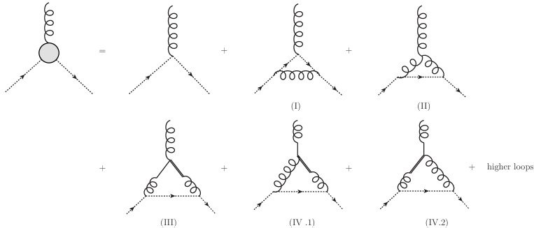
Figure 1: Feynman diagram expansion up to one-loop order for the ghost-gluon vertex in the Refined Gribov-Zwanziger. Dashed lines represent ghosts and antighosts, while the curly lines stand for gluons. Full simple and double lines, that only appear in mixed propagators, correspond to the auxiliary fields $\varphi$ and $\bar{\varphi}$, respectively. The roman numbers identifying the one-loop diagrams will be used as reference in the results section and in the appendices. The diagrams were generated by means of the Jaxodraw interface Binosi et al. (2009).

Before proceeding, let us remark that since the RGZ action contains bilinear couplings between fields, the theory contains mixed propagators, such as $\left\langle{A\varphi}\right\rangle$ and $\left\langle{A\bar{\varphi}}\right\rangle$. Therefore, the relation between connected and 1PI functions has to take such mixed propagators into account. This is made explicit in the Feynman diagrams of Fig. 1. Such mixed propagators and vertices involving Zwanziger’s auxiliary fields $\varphi$ and $\bar{\varphi}$ as well as their fermionic counterparts $\omega$ and $\bar{\omega}$, arise as a consequence of the local formulation of the Gribov horizon . We give further details for the interested reader in Appendix B.

Since the tree-level mixed propagator is such that

$$\langle A_{\mu}^{a}(p)\varphi_{\nu}^{bc}(-p)\rangle = \frac{-ig\gamma^{2}f^{abc}}{p^{4}+p^{2}(m^{2}+M^{2})+m^{2}M^{2}+2Ng^{2}\gamma^{4}}P^{\perp}_{\mu\nu}(p),$$ (15)

the one-loop connected function (14) can then be decomposed as

$$\left\langle{A_{\nu}^{a}(k)\,\bar{c}^{b}(p)\,c^{c}(q)}\right\rangle =G(p)G(q)D_{AA}(k)P^{\perp}_{\mu\nu}(k)\left\{\Gamma_{A^{a}_{\mu}\bar{c}^{b}c^{c}}(k,p,r)+\frac{2g\gamma^{2}f^{ade}}{k^{2}+M^{2}}\Gamma_{\bar{c}^{b}c^{c}\varphi^{de}_{\mu}}(k,p,r)\right\}_{q=-p-k},$$ (16)

where

$$P^{\perp}_{\mu\nu}(p)=\delta_{\mu\nu}-\frac{p_{\mu}p_{\nu}}{p^{2}}$$ (17)

is the transverse projector, and the relevant 1PI functions are

$$\Gamma_{A^{a}_{\nu}\bar{c}^{b}c^{c}}(k,p,r):=\frac{\delta^{3}\Gamma}{\delta A_{\nu}^{a}(-k)\delta\bar{c}^{b}(-p)\delta c^{c}(-q)}$$ (18)

and

$$\Gamma_{\bar{c}^{b}c^{c}\varphi^{de}_{\mu}}(k,p,r):=\frac{\delta^{3}\Gamma}{\delta\bar{c}^{b}(-p)\delta c^{c}(-q)\delta\varphi_{\nu}^{de}(-k)}.$$ (19)

Note the presence of the $\Gamma_{\bar{c}c\varphi}$ and $\Gamma_{\bar{c}c\bar{\varphi}}$ vertex functions in the RGZ theory. They are zero at tree-level. In the case of $\Gamma_{\bar{c}c\varphi}$ its first nontrivial terms are given by diagrams (IV.1) and (IV.2) of fig. 1. Notice that, since $\Gamma_{\bar{c}c\varphi}=\Gamma_{\bar{c}c\bar{\varphi}}$, in fig. 1 we have included the diagrams associated with the former quantity only. The contribution of $\Gamma_{\bar{c}c\bar{\varphi}}$ to $\left\langle{A_{\nu}^{a}(k)\,\bar{c}^{b}(p)\,c^{c}(q)}\right\rangle$ is introduced by multiplying the contribution of $\Gamma_{\bar{c}c\varphi}$ by a factor of two, as can be observed in eq. 16.

The tensorial structure of the ghost-gluon 1PI vertex function is given by

$$\Gamma_{A^{a}_{\mu}\bar{c}^{b}c^{c}}(k,p,r)=-igf^{abc}\large[p_{\mu}B_{1}(k,p)+k_{\mu}B_{2}(k,p)\large],$$ (20)

where we adopt the same notation as in Aguilar et al. (2019) and consider all momenta as incoming. At tree-level, the scalar structure functions are $B_{1}(k,p)=1$ and $B_{2}(k,p)=0$.

On the other hand, the contraction of the $\Gamma_{\varphi\bar{c}c}$ function with the antisymmetric color structure constant tensor can be decomposed as

$$f^{ade}\Gamma_{\bar{c}^{b}c^{c}\varphi^{de}_{\mu}}(k,p,r)=-igf^{abc}\left(p_{\mu}C_{1}(k,p)+k_{\mu}C_{2}(k,p)\right)-igd^{abc}\left(p_{\mu}C^{\prime}_{1}(k,p)+k_{\mu}C^{\prime}_{2}(k,p)\right)$$ (21)

Since this combination must be antisymmetric in the color indices $b$ and $c$ (due to the fact that the ghost fields are grassmannian), the coefficient of the totally symmetric tensor $d^{abc}$ must vanish identically, i.e., $C^{\prime}_{1}=C^{\prime}_{2}=0$. As a result, we may write the one-loop connected three-point function as

$$\left\langle{A_{\mu}^{a}(k)\,\bar{c}^{b}(p)\,c^{c}(q)}\right\rangle = -igp_{\nu}\,f^{abc}G(p)G(p+k)D_{AA}(k)P^{\perp}_{\mu\nu}(k)\left\{B_{1}(k,p)+\frac{2g\gamma^{2}}{k^{2}+M^{2}}C_{1}(k,p)\right\},$$ (22)

where the longitudinal scalar functions $B_{2}$ and $C_{2}$ are no longer present (in the Landau gauge) due to the transversality of the gluon propagator.

In order to make contact with results from Monte Carlo lattice simulations, let us consider the scalar quantity Cucchieri et al. (2006)

$$G^{CCA}(p,k) \equiv\frac{\Gamma_{(A\bar{c}c,tree)}^{abc}\,{}_{\mu}(k,p,-k-p)\left\langle{A_{\mu}^{a}(k)\,\bar{c}^{b}(p)\,c^{c}(-k-p)}\right\rangle}{\Gamma_{(A\bar{c}c,tree)}^{abc}\,{}_{\mu}(k,p,-p-k)\Gamma_{(A\bar{c}c,tree)}^{abc}\,{}_{\nu}(k,p,-p-k)P_{\mu\nu}(k)G(p)G(p+k)D_{AA}(k)}$$

$$=B_{1}(k,p)+\frac{2g\gamma^{2}}{k^{2}+M^{2}}C_{1}(k,p),$$ (23)

which from now on we denote as the ghost-gluon vertex dressing function.

There are clearly some differences between perturbative YM and RGZ calculations of the vertex function. The first of them is the modification of the gluon propagator brought about by the restriction to the Gribov horizon, which can be understood as the appearance of a pair of generally complex conjugate poles. A second difference is the presence of the tree-level $A\bar{\varphi}\varphi$ vertex, which couples the gluon to the auxiliary Zwanziger fields. This allows not only diagrams with auxiliary fields running in the internal loops, but also in the external legs, as long as the external propagator is a mixed one like, for example, $\left\langle{A\varphi}\right\rangle$. This possibility is realized in (16), giving rise to the contributions $\Gamma_{\varphi\bar{c}c}$ and $\Gamma_{\bar{\varphi}\bar{c}c}$, not present in perturbative YM theory. Furthermore, note that these mixed contributions only appear from one-loop order onwards, as such vertices are absent from the classical action (II). Being finite, they do not spoil the stability of the action, in agreement with the Quantum Action Principle Piguet and Sorella (1995). Finally, we note that the presence of such vertices involving the auxiliary Zwanziger fields can be thought as effective momentum-dependent gluonic interaction terms. This claim can be explicitly shown to be true, starting from the tree level action, by considering the nonlocal version of the RGZ theory (whose action can be obtained from (II) by integrating out the Zwanziger auxiliary fields) and expanding the inverse of the Faddeev-Popov operator in powers of the coupling. In this regard, we note that it is reasonable to consider the RGZ effective action not simply as an effective model with propagators given by a ratio of polynomials, but rather a renormalizable effective theory with nontrivial gluonic propagators and self-interactions, which are related to each other.

As a final remark, let us note that all diagrams contributing to the ghost-gluon vertex are finite in the RGZ theory, just as in the perturbative Yang-Mills theory. In fact, the mixed propagators present in diagrams (III) and (IV) make the diagrams even more ultraviolet convergent than the usual YM diagrams (I) and (II). This can be easily seen from the form of the $\left\langle{A\varphi}\right\rangle$ propagator (15).

III.2 The soft gluon limit

The calculation of the ghost-gluon vertex for any momentum requires the calculation of the diagrams shown in fig. 1. Since this calculation is rather long to be performed manually, in a previous work some of us considered the soft-gluon limit of $\Gamma_{A\bar{c}c}$, i.e., the limit in which the gluon momentum $k\rightarrow 0$ Mintz et al. (2018).

In the soft gluon limit, each diagram takes a simplified form and furthermore, since diagram (IV) of fig. 1 is proportional to the gluon momentum (and it is finite), it vanishes for $k\rightarrow 0$. In this limit, the one-loop correction for the vertex, which has been explicitly calculated in Mintz et al. (2018), reads

$$[\Gamma_{A\bar{c}c}^{(1)}(0,p,-p)]^{abc}_{\mu} = ig^{3}\frac{Nf^{abc}}{2}\bigg{\{}R_{+}J_{\mu}(a_{+};p)+R_{-}J_{\mu}(a_{-};p)+2R_{+}^{2}K_{\mu}(a_{+},a_{+};p)+2R_{-}^{2}K_{\mu}(a_{-},a_{-};p)+$$ (24)

$$\left.+4R_{+}R_{-}K_{\mu}(a_{+},a_{-};p)+\frac{N}{2}\left(\frac{g\gamma^{2}}{a_{+}^{2}-a_{-}^{2}}\right)^{2}\left[K_{\mu}(a_{+},a_{+};p)+K_{\mu}(a_{-},a_{-};p)-\right.\right.$$

$$-2K_{\mu}(a_{+},a_{-};p)\big{]}\bigg{\}}\,,$$

where

$$a_{+}^{2}\equiv\frac{m^{2}+M^{2}+\sqrt{(m^{2}-M^{2})^{2}-4\lambda^{4}}}{2},$$

$$a_{-}^{2}\equiv\frac{m^{2}+M^{2}-\sqrt{(m^{2}-M^{2})^{2}-4\lambda^{4}}}{2},$$

with $\lambda^{4}\equiv 2Ng^{2}\gamma^{4}$, and the integral

$$J_{\mu}(m_{1};p)\equiv\int\frac{d^{d}q}{(2\pi)^{d}}\,\frac{1}{q^{2}}\frac{1}{q^{2}+m_{1}^{2}}\frac{p^{2}q^{2}-(p\cdot q)^{2}}{[(q-p)^{2}]^{2}}\,(q-p)_{\mu},$$ (25)

is related to diagram (I) while

$$K_{\mu}(m_{1},m_{2};p) \equiv \int\frac{d^{d}q}{(2\pi)^{d}}\frac{1}{(q+p)^{2}}\frac{1}{q^{2}+m_{1}^{2}}\frac{1}{q^{2}+m_{2}^{2}}\,\left[\frac{q^{2}p^{2}-(p\cdot q)^{2}}{q^{2}}\right]q_{\mu}\,$$ (26)

appears in diagrams (II) and (III). The incoming antighost momentum is given by $p$. Therefore, the ghost momentum is $-p$, since $k=0$ in the soft-gluon limit. The massive parameters $-a_{\pm}^{2}$ are the, generally complex, poles of the RGZ gluon propagator (42) and $R_{\pm}$ are their corresponding residues. It is worth pointing out that the last terms in eq. (24) come from diagram (III) in fig. 1 which is absent in standard YM theories, being proportional to the Gribov parameter.

As a last remark, let us note an important feature of the $\Gamma_{A\bar{c}c}$ vertex function in the RGZ theory: it explicitly respects the so-called Taylor kinematics, i.e.,

$$(\Gamma_{A\,\bar{c}\,c})^{abc}_{\mu}(p,0,-p)=0\,,$$ (27)

and the so-called non-renormalization theorem of the ghost-gluon vertex

$$(\Gamma_{A\,\bar{c}\,c})^{abc}_{\mu}(-p,p,0)=-igf^{abc}p_{\mu},$$ (28)

which are the same in the RGZ framework as in perturbative YM theory Taylor (1971). These are direct consequences of the Ward identities of the action (II).

IV The one-loop RGZ ghost-gluon vertex for generic momentum configurations

IV.1 Feynman diagrams

It is clear from eq. 23 that the ghost-gluon vertex dressing function relates to two 1PI structures. Diagrams (I)-(III) from fig. 1 contribute to $\Gamma_{A\bar{c}c}$, while the forth diagram contributes to $\Gamma_{\varphi\bar{c}c}$.

Their expressions in terms of the Feynman rules from appendix A, following the numbering from fig. 1, are:

$$D_{(I)}=-ig^{3}\frac{N}{2}f^{abc}p_{\nu}(p+k)_{\rho}\int\frac{d^{d}q}{(2\pi)^{d}}q_{\mu}P^{\perp}_{\nu\rho}(q+p)D_{AA}(q+p)D_{\bar{c}c}(q-k)D_{\bar{c}c}(q)\,,$$

$$D_{(II)}=-ig^{3}\frac{N}{2}f^{abc}p_{\eta}(p+k)_{\omega}\int\frac{d^{d}q}{(2\pi)^{d}}\left(-2k_{\rho}\delta_{\mu\nu}+2k_{\nu}\delta_{\mu\rho}+(2q-k)_{\mu}\delta_{\nu\rho}\right)P^{\perp}_{\nu\eta}(q)P^{\perp}_{\rho\omega}(q-k)D_{AA}(q)D_{AA}(q-k)D_{\bar{c}c}(q+p)\,,$$

$$D_{(III)}=ig^{3}\frac{N^{2}}{4}f^{abc}(g\gamma^{2})^{2}p_{\nu}(p+k)_{\rho}\int\frac{d^{d}q}{(2\pi)^{d}}(2q-k)_{\mu}P^{\perp}_{\rho\eta}(q-k)P^{\perp}_{\nu\eta}(q)D_{A\varphi}(q-k)D_{A\varphi}(q)D_{\bar{c}c}(q+p)\,,$$

$$f^{ade}D_{(IV.1)}=ig^{3}\frac{N^{2}}{4}f^{abc}(g\gamma^{2})p_{\eta}k_{\omega}(p+k)_{\sigma}\int\frac{d^{d}q}{(2\pi)^{d}}P^{\perp}_{\sigma\mu}(q-k)P^{\perp}_{\eta\omega}(q)D_{A\varphi}(q-k)D_{AA}(q)D_{\bar{c}c}(q+p)\,,$$

$$f^{ade}D_{(IV.2)}=-ig^{3}\frac{N^{2}}{4}f^{abc}(g\gamma^{2})p_{\sigma}k_{\omega}(p+k)_{\eta}\int\frac{d^{d}q}{(2\pi)^{d}}P^{\perp}_{\sigma\mu}(q)P^{\perp}_{\eta\omega}(q-k)D_{A\varphi}(q)D_{AA}(q-k)D_{\bar{c}c}(q+p)\,,$$ (29)

where $D_{XY}(q)$ designates the propagator of momentum $q$ between the fields $X$ and $Y$.

The above Feynman integrals depend on two external momenta, p and k, and feature only one Lorentz index which is not contracted, $\mu$. As a result, all of them can be expressed as $F(p^{2},k^{2},p\cdot k,M^{2},m^{2},\lambda)p_{\mu}+H(p^{2},k^{2},p\cdot k,M^{2},m^{2},\lambda)k_{\mu}$, where $F$ and $H$ are scalar integrals. In the first stage of our computation we found the corresponding scalar integrals for each diagram and evaluated the color factors by means of the ColorMath package Sjödahl (2013).

In a second stage, we reduced the scalar integrals to one-loop master integrals Passarino and Veltman (1979) of the type

$$A_{x}\equiv\int_{q}G_{x}(q^{2}),$$ (30)

$$B_{xy}(p^{2})\equiv\int_{q}G_{x}(q^{2})G_{y}((p-q)^{2}),$$ (31)

$$C_{xyz}(p^{2},k^{2},p\cdot k)\equiv\int_{q}G_{x}(q^{2})G_{y}((p-q)^{2})G_{z}((k-q)^{2}),$$ (32)

where

$$\int_{q}\equiv\int 16\pi^{2}\mu^{2\epsilon}\frac{d^{d}q}{(2\pi)^{d}},$$ (33)

with $\epsilon=\frac{4-d}{2}\geq 0$ and

$$G_{x}(q^{2})\equiv\frac{1}{q^{2}+x},$$ (34)

where $x$ is a “mass” squared (which may be complex, in our case). In the case of the RGZ theory $x\in\{0,M^{2},a_{+}^{2},a_{-}^{2}\}$. The mass dimension of the gauge coupling, defined as $\mu^{\epsilon}$, is absorbed into the definition of the master integrals. More specifically, as the dressing function $G^{CCA}$ is proportional to $g^{2}$, we include the respective mass dimension, $\mu^{2\epsilon}$, in the definition given by eq. (33).

We implemented the reduction to master integrals using an algorithm in Mathematica based on the Fire package Smirnov and Chuharev (2020). The reduction for each diagram is presented in a supplementary material. The analysis is performed for an arbitrary number of colors $N$ with the purpose of comparing with alternative approaches, both for the SU(2) and SU(3) gauge groups.

Once the reduction is finished we need to compute the one-loop master integrals. For both $A$ and $B$ there are well-known analytic results (see, for instance, ref. Martin (2003)). In the case of the master integral $C$, when needed, we evaluated it numerically.

We note here that since all one-loop diagrams are finite no renormalization factors are needed.

IV.2 Kinematic configurations

Concerning the particular kinematic configurations we will address in this article, it is convenient to recall that three-point correlation functions depend on two external momenta. Because of translational and rotational invariance such dependence can be described by means of three independent kinematic variables. We choose the magnitudes of the antighost and gluon momentum, $p$ and $k$, along with the scalar product $\textit{p}\cdot\textit{k}$.

In this paper we aim at extending the analysis of the ghost-gluon vertex within the RGZ framework, initially explored in Mintz et al. (2018), beyond the soft gluon limit, to include arbitrary kinematic configurations. We focus on the specific kinematic setups for which we have access to lattice simulations, namely the symmetric and orthogonal configurations.

The symmetric configuration is characterized by equal momentum magnitudes for the external antighost and gluon legs, $p=k$, forming an angle of $\theta=\pi/3$. On the other hand, the orthogonal configuration refers to external momenta perpendicular to each other, $\theta=\pi/2$. Within this work, our reference to the orthogonal configuration includes the additional condition $p=k$.

IV.3 Numerical values of the RGZ parameters

Within the RGZ framework, there are four parameters: $M$ and $m$, that are mass parameters associated with dimension two condensates, the Gribov parameter $\gamma$ and the gauge coupling $g$. For the sake of convenience, we introduce the parameter $\lambda^{4}=2Ng^{2}\gamma^{4}$, which we will employ in place of $\gamma$.

In principle, the three massive parameters could be determined self-consistently using the Gribov gap equation and minimizing the effective potential of the theory with respect to two condensates. Here, however, we shall fix these parameters using lattice input. The parameters $M,m$ and $\lambda$ at tree-level were determined for SU(2) in Cucchieri et al. (2012) and for SU(3) in Oliveira and Silva (2012), by fitting the lattice data of the gluon propagator from YM theory with an analytic expression of the form:

$$D(p^{2})=\frac{p^{2}+a}{p^{4}+bp^{2}+c},$$ (35)

where $a$, $b$ and $c$ are constants. This analytic form coincides with the tree-level gluon propagator of the RGZ framework,

$$D(p^{2})=\frac{p^{2}+M^{2}}{p^{4}+(M^{2}+m^{2})p^{2}+M^{2}m^{2}+\lambda^{4}},$$ (36)

allowing for the extraction of $m$, $M$ and $\lambda$ from eq. (35). The obtained values are displayed in table 1.

Gauge group	$M^{2}$ (${\rm GeV}^{2}$)	$m^{2}$ (${\rm GeV}^{2}$)	$\large\lambda$ (${\rm GeV}$)
SU(2) - Ref.Cucchieri et al. (2012)	2.51	-1.92	1.52
SU(3) - Ref.Oliveira and Silva (2012)	4.47	-3.77	2.04

Table 1: RGZ parameters fitted from lattice results for SU(2) Cucchieri et al. (2012) and SU(3) Oliveira and Silva (2012).

IV.4 Toy model of the running coupling

The gauge coupling $g$ is to be determined by fitting the RGZ ghost-gluon vertex to available lattice simulations. To that end, it is useful to introduce the relative error between the RGZ output and the lattice data,

$$\chi^{2}\equiv\frac{1}{N_{\text{latt}}^{2}}\sum_{i}^{N_{\text{latt}}}\Bigg{(}\frac{G_{\text{RGZ}}(p_{i})-G_{\text{latt}}(p_{i})}{G_{\text{latt}}(p_{i})}\Bigg{)}^{2},$$ (37)

where $N_{\text{latt}}$ is the number of lattice data points, $G_{\text{RGZ}}$ and $G_{\text{latt}}$ refer to the RGZ and the numerical results, respectively.

Firstly, we simply investigate at a qualitative level the variation of the dressing function $G^{CCA}$ as we change fixed values of $g$. As we will see, this is enough to reproduce either the IR or the UV but not both regimes at the same time. Most likely this is due to the presence of large logarithms in the UV domain, which spoils the validity of perturbation theory. This problem can be overcome by introducing the running of the various parameters of the RGZ framework and choosing a renormalization scale of the same order of the external momentum: $\mu\sim p$. To achieve this we would need to evaluate the two-point functions of the theory by introducing an infrared-safe scheme, of the type introduced in Pelaez et al. (2013) for instance.

However, this sort of approach exceeds the scope of the present article. Instead, we keep the constant values provided in table 1 and make use of a toy model for the renormalization group (RG) flow of the gauge coupling, motivated by the standard Yang-Mills one loop $\beta$-function in the Modified Minimal Subtraction Scheme,

$$g^{2}(\mu)=\frac{g_{0}^{2}}{1+\frac{11}{3}N\frac{g_{0}^{2}}{16\pi^{2}}\log(\frac{\mu^{2}+\Lambda^{2}}{\Lambda^{2}})},$$ (38)

and choose $\mu=p$. The parameter $\Lambda$ is introduced to regularize the IR by freezing the running of the gauge coupling for momentum scales much smaller than $\Lambda$, where we expect the effects of the renormalization flow to be less relevant. The fits of $G^{CCA}$ from the RGZ framework to lattice data are carried out by selecting the parameters $g_{0}$ and $\Lambda$ that minimize $\chi$.

V Results

In this section we show the results for the ghost-gluon vertex dressing function, $G^{CCA}$, for both the gauge groups SU(2) and SU(3) in four spacetime dimensions. We compare our results with lattice simulations and outcomes from the CF model and DSE. Additionally, we show the contributions of each Feynman diagram to the final results.

V.1 SU(2)

We begin by analyzing the ghost-gluon vertex dressing function $G^{CCA}$ for the SU(2) gauge group in the symmetric and orthogonal kinematic configurations, as well as in the case of the soft gluon limit. The latter case was previously investigated in Mintz et al. (2018). However, for completeness and because the analysis we perform in this article differs slightly from the one developed in Mintz et al. (2018), we include those results here as well.

V.1.1 Fitting the ghost-gluon vertex dressing function

In fig. 2 we see the dressing function $G^{CCA}$ for various fixed values of the gauge coupling $g$ at one-loop order from the RGZ framework. As for the symmetric and orthogonal kinematic configurations it is clear that, although we find values of the coupling that show a very good agreement with lattice data either at the IR (pink curve) or the UV (purple curve), we are unable to reconcile both regions simultaneously. This is reasonable, as we are not taking into account the RG effects.

Interestingly, in the case of the soft gluon limit it seems that it is possible to describe the lattice data for the whole range of momenta with a constant value of gauge coupling (red curve). The quality of the fit, though, must be taken carefully due to the relatively large dispersion of the lattice data, specially at low momenta.

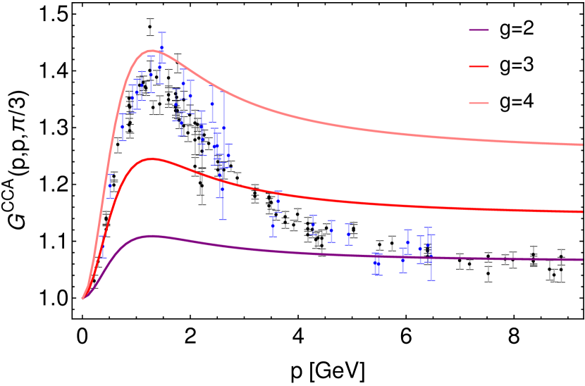
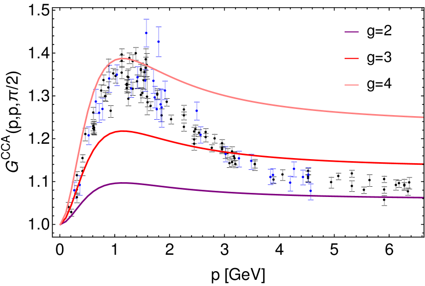
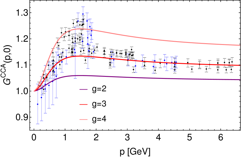
Figure 2: The SU(2) scalar function $G^{CCA}$ as a function of the antighost external momentum in three distinct configurations: the symmetric (top left), orthogonal (top right) and the soft gluon limit (bottom) for various values of a fixed gauge coupling. Blue and black points refer to lattice data extracted from refs. Cucchieri et al. (2008) and Maas (2020), respectively.

To investigate to which extent the RG flow is capable of reducing the discrepancy between the lattice data and the RGZ fit, we incorporate the toy model of the running coupling shown in eq. (38). The level curves illustrating the dependence of the relative error defined in eq. 37 on the parameters $g_{0}$ and $\Lambda$ are depicted in fig. 3. We notice that the regions minimizing $\chi$ are very similar for the symmetric and orthogonal configurations. These regions are also compatible with the level curves of $\chi$ observed in the soft gluon limit, though the area of minimum error appears more extensive. This discrepancy could stem from a greater uncertainty and dispersion of the lattice data in the soft gluon limit compared to the data from the symmetric and orthogonal setups.

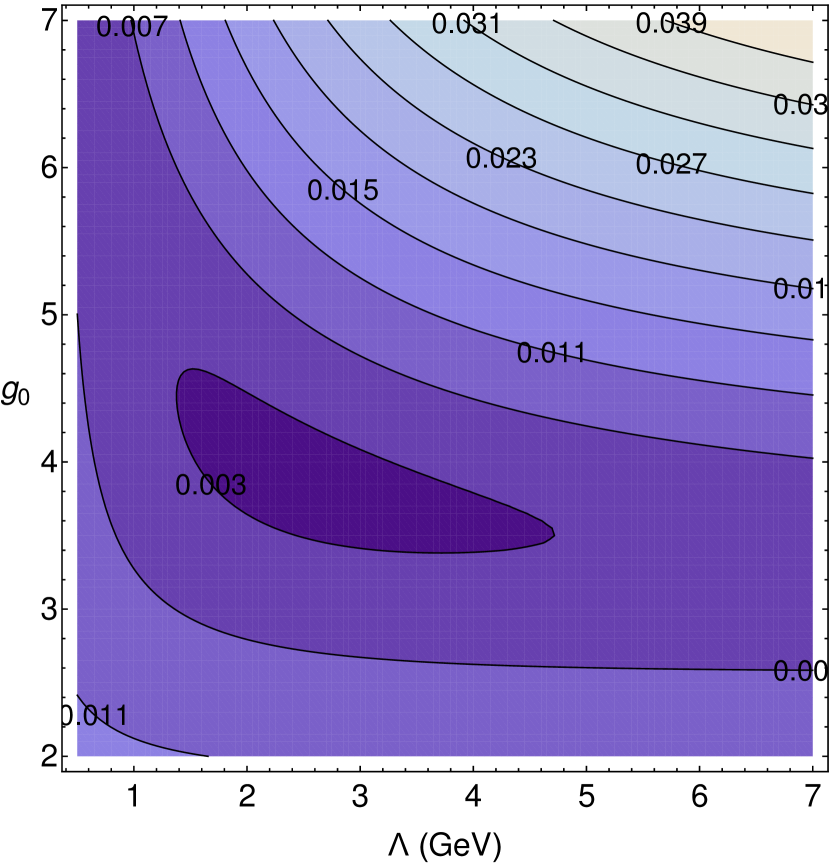
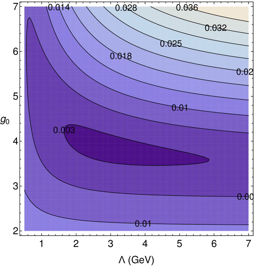
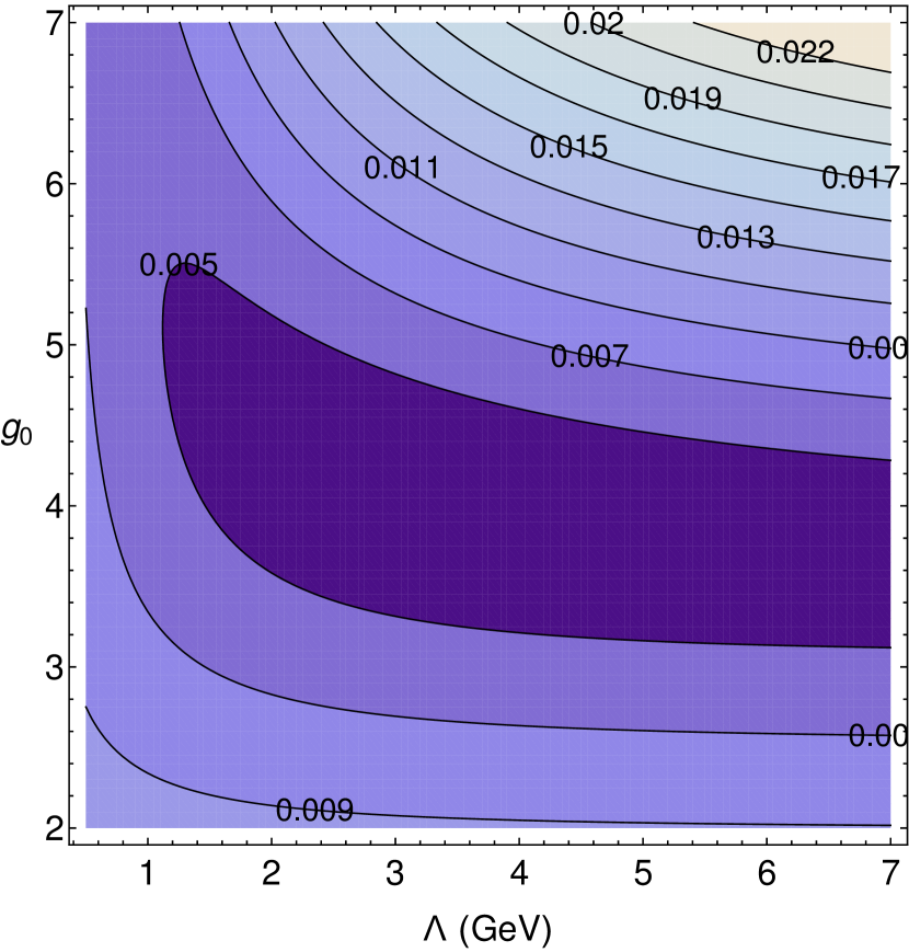
Figure 3: Level curves of the relative error $\chi$, defined in eq. 37, as a function of the parameters $\Lambda$ and $g_{0}$, for the symmetric (left) and orthogonal (center) configurations as well as the soft gluon limit (right) for the SU(2) case.

The parameters that minimize $\chi$ in each kinematic configuration are displayed in table 2. Additionally, we incorporate the values of $g_{0}$ and $\Lambda$ that minimize the deviation between the lattice data and the RGZ output across all kinematic configurations simultaneously. These values are computed by minimizing the collective error, $\chi_{\text{joint}}$, which we define as

$$\chi_{\text{joint}}^{2}\equiv\frac{\chi_{\text{sym.}}^{2}+\chi_{\text{orth.}}^{2}+\chi_{\text{soft}}^{2}}{3},$$ (39)

where $\chi_{\text{sym.}}$, $\chi_{\text{orth.}}$ and $\chi_{\text{soft}}$ refer to the relative error of the symmetric, orthogonal and the soft gluon configurations, respectively.

SU(2) fits for different configurations

Kinematic configuration	$g_{0}$	$\Lambda$ (${\rm GeV}$)	$\chi$
Symmetric	3.90	2.40	0.0029
Orthogonal	3.85	2.90	0.0028
Soft gluon	3.95	3.90	0.0044
Sym. + Orth. + Soft	3.90	2.75	0.0036

Table 2: Values of the parameters $g_{0}$ and $\Lambda$ that minimize the discrepancy between the RGZ outcome of the function $G^{CCA}$ and the corresponding lattice data for various kinematic configurations in the SU(2) case. The last row refers to the values that minimize the joint error $\chi_{\text{joint}}$, defined in eq. 39.

The parameters that minimize $\chi_{\text{joint}}$ are $g_{0}=3.90$ and $\Lambda=2.75\ {\rm GeV}$. Using these parameter values, we collect in table 3 the $\chi$ values for each kinematic configuration, which indicate that the deterioration of the individual fits for each configuration is minimal when performing the collective fit. The corresponding plots are shown in fig. 4.

SU(2) joint fit

Kinematic configuration	$\chi$
Symmetric	0.0031
Orthogonal	0.0028
Soft gluon	0.0046

Table 3: Values of the parameters $\chi$ of each kinematic configuration corresponding to the parameters that minimize the joint error $\chi_{\text{joint}}$, $g_{0}=3.90$ and $\Lambda=2.75{\rm GeV}$, in the SU(2) case.

We observe that the fit of fig. 4 exhibits a strong agreement with lattice simulations across all kinematic configuration. However, the UV tails of the RGZ curves consistently fall above the lattice data points. This discrepancy could arise from the larger number of lattice points in the IR region compared to the UV domain, emphasizing the agreement between the RGZ result and lattice data in the low momentum zone at the expense of deteriorating the fit in the UV.

In fig. 4 we include also the results of the Curci-Ferrari (CF) model in Landau gauge at one- and two-loop accuracy. The outcomes from both frameworks, CF and RGZ, are consistent. Nonetheless, within this analysis, comparing both approaches must be done with care due to two reasons. Firstly, concerning the symmetric and orthogonal configurations, the CF curves of $G^{CCA}$ are pure predictions of the model, while the RGZ curves represent a global fit of the lattice data. This renders the comparison fairer in the case of the soft-gluon limit, where the results from the CF approach come from a global fit of the two-point functions and $G^{CCA}$. Secondly, due to the complexity of the RGZ approach, we employ a simplified model for the RG flow of the gauge coupling, disregarding the RG effects of other parameters of the theory, which could potentially alter the final result.

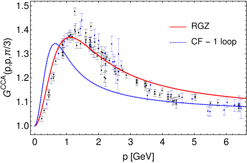
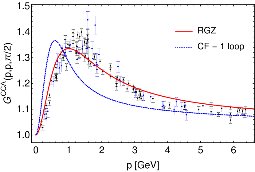
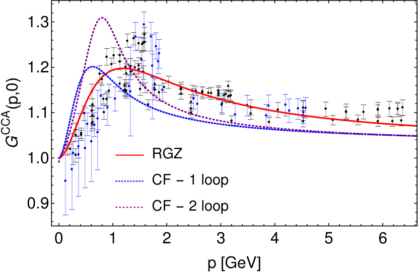
Figure 4: The scalar function $G^{CCA}$ for the SU(2) case as a function of the antighost external momentum in three distinct configurations: the symmetric (top left), orthogonal (top right) and the soft gluon limit (bottom). The red curve represents the RGZ fit of the lattice data by using the toy model of eq. 38 for the gauge coupling. The values of the parameters, $\Lambda=2.75$ GeV and $g_{0}=3.9$, are chosen to minimize the joint relative error $\chi_{\text{joint}}$. Regarding the symmetric and orthogonal configurations, the blue curve is the prediction from the CF model at one-loop order Pelaez et al. (2013). In the soft gluon limit, the CF results are global fits of the gluon and ghost propagators along with the dressing function $G^{CCA}$ at one- and two-loop order Barrios et al. (2020). Blue and black points refer to lattice data extracted from refs. Cucchieri et al. (2008) and Maas (2020), respectively.

V.1.2 Contribution of each diagram to the $G^{CCA}$ fit

We now examine the contribution of each diagram to the full result of $G^{CCA}$ in the symmetric and orthogonal configurations, as well as in the soft-gluon limit. The result is presented in fig. 5, where we follow the numbering from fig. 1. As for the quantity we denote as diagram (IV), it corresponds to the full contribution $\frac{2g\gamma^{2}f^{ade}}{k^{2}+M^{2}}\Gamma_{\bar{c}^{b}c^{c}\varphi^{de}_{\mu}}(k,p,r)$, see eq. 16.

We note that genuinely RGZ diagrams, (III) and (IV), represent a small contribution at one-loop order as compared to the largest contribution of diagram (I) and, to a lesser degree, diagram (II). This is in agreement with the results obtained by CF model Tissier and Wschebor (2010, 2011); Pelaez et al. (2013); Peláez et al. (2014, 2015); Gracey et al. (2019); Peláez et al. (2021); Figueroa and Peláez (2022); Barrios et al. (2020, 2021, 2022) where only QCD-like diagrams with massive gluons are taken into account. Interestingly, the effect of diagrams (III) and (IV) is a reduction of the peak of $G^{CCA}$, at around $p=1.5$ GeV.

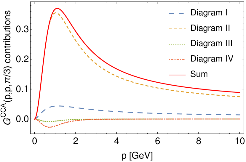
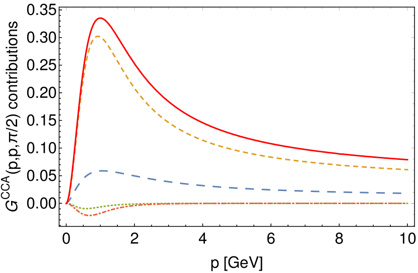
Figure 5: Contribution of each diagram to $G^{CCA}$ for the SU(2) case in three distinct configurations: the symmetric (top left), orthogonal (top right) and the soft gluon limit (bottom), using the gauge coupling described by eq. 38. The values of the parameters, $\Lambda=2.75$ GeV and $g_{0}=3.90$, are chosen to minimize the joint relative error $\chi_{\text{joint}}$. The convention of colors and line-styles in the orthogonal and soft configurations is the same as the symmetric case. The red curve is the sum of all diagrams. The numbering of the diagrams is provided in fig. 1. Diagram (IV) refers to the full contribution $\frac{2g\gamma^{2}f^{ade}}{k^{2}+M^{2}}\Gamma_{\bar{c}^{b}c^{c}\varphi^{de}_{\mu}}(k,p,r)$.

V.2 SU(3)

In this section we replicate the analysis performed for the SU(2) gauge group but for the case of the SU(3) gauge group. Yet, the conclusions derived from this analysis will be more restricted compared to the SU(2) case due to the lack of lattice data available in kinematic configurations other than the soft gluon scenario.

In what follows we present results for the same configurations analyzed in the previous section, i.e. the symmetric and orthogonal configurations as well as in the soft gluon limit. Although the only configuration with available lattice data is the latter, the other configurations are valuable for comparison with alternative approaches in the continuum.

V.2.1 Fitting the ghost-gluon vertex dressing function

In fig. 6 we see $G^{CCA}$ as a function of the antighost momentum for the symmetric and orthogonal configurations as well as in the soft gluon limit. Similarly to what we observed in the case of the SU(2) gauge group, as for the soft gluon limit it seems that we are capable of reproducing the lattice data by using a fixed value of the gauge coupling $g$, as was already pointed out in Mintz et al. (2018).

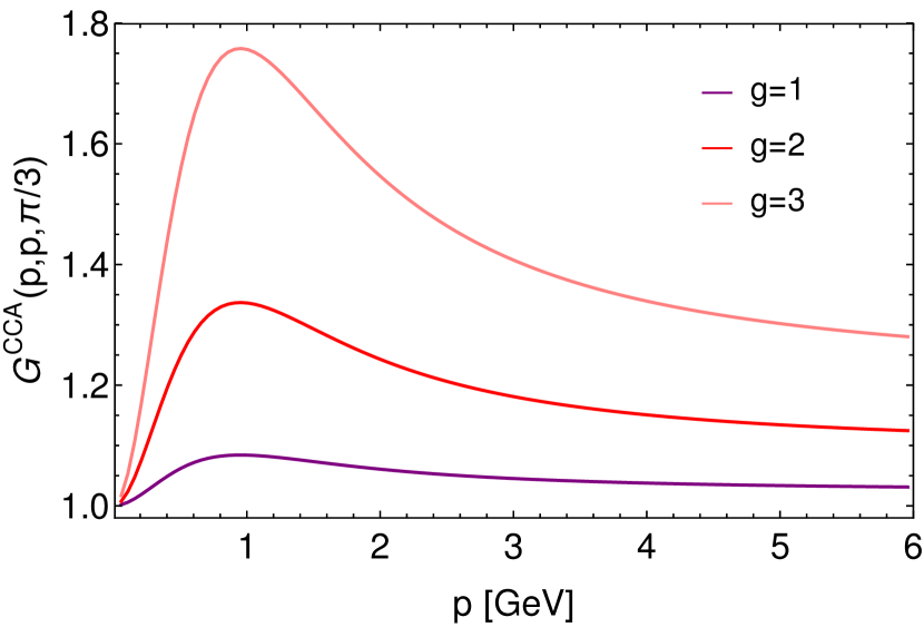
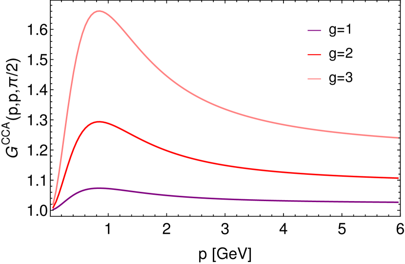
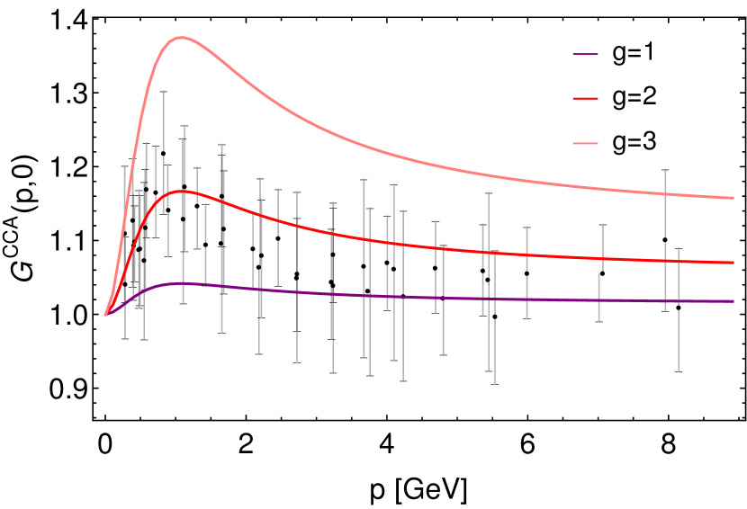
Figure 6: The scalar function $G^{CCA}$ for the SU(3) case as a function of the antighost external momentum in three distinct configurations: the symmetric (top left), orthogonal (top right) and the soft gluon limit (bottom) for various values of a fixed gauge coupling. The lattice data were extracted from the plots in Ilgenfritz et al. (2007) using WebPlotDigitizer Rohatg . We estimated the error of the extraction procedure to be at most 0.8%.

.

It is worth examining how the deviation between the RGZ outcome and lattice data is modified as we change the parameters $\Lambda$ and $g_{0}$ when using the simplified model (eq. (38)). The level curves illustrating this dependence are depicted in fig. 7, displaying an error $\chi$ independent of the scale $\Lambda$ as long as the values of $g_{0}$ remain moderate. This reinforces our previous observation that, within the soft gluon limit, the RGZ framework effectively reproduces lattice data with a fixed value of $g$. Nevertheless, as we aim to analyze the symmetric and orthogonal configurations as well, which are likely sensitive to RG effects, in what follows we continue employing the scale-dependent gauge coupling defined by eq. 38.

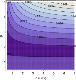
Figure 7: Level curves of the relative error $\chi$, defined in eq. 37, as a function of the parameters $\Lambda$ and $g_{0}$, as for the soft gluon limit in the SU(3) case.

.

In analogy to our analysis for the SU(2) case, in order to find the best fit to lattice data, we find the parameters $\Lambda$ and $g_{0}$ that minimize the relative error $\chi$. In the soft gluon setup, the minimum of $\chi$ corresponds to $\Lambda=0.70$ GeV and $g_{0}=2.15$, with a relative error of $\chi=0.0040$. The resulting plots are depicted in fig. 8.

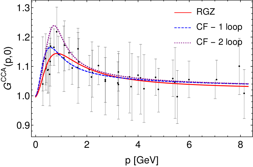
Figure 8: The scalar function $G^{CCA}$ for the SU(3) case as a function of the antighost external momentum in three distinct configurations: the symmetric (top left), orthogonal (top right) and the soft gluon limit (bottom). The red curve corresponds to the RGZ fit of the lattice data, by utilizing the toy model of eq. 38 for the gauge coupling. Parameters $\Lambda=0.70$ GeV and $g_{0}=2.15$ were chosen to minimize the joint relative error with the lattice data in the case of the soft gluon limit. Lattice data are extracted from Ilgenfritz et al. (2007). We compare the results with other approaches in the continuum. Specifically with $G^{CCA}$ obtained from DSE, considering the bare (DSE - I) and the dressed three-gluon vertex (DSE - II) Aguilar et al. (2019) and $G^{CCA}$ from the CF model at one- and two-loop order Pelaez et al. (2013); Barrios et al. (2020).

We note that our results for $G^{CCA}$ are consistent with the outcomes of the CF model Pelaez et al. (2013); Barrios et al. (2020) and DSE Aguilar et al. (2019). Furthermore, the RGZ fit shows a strong agreement with simulations, resembling the results obtained with a fixed value of the gauge coupling. Interestingly, while the UV tails of the DSE and CF curves overlap in the UV, the UV tails from the RGZ curves fall more rapidly in comparison.

V.2.2 Contribution of each diagram to the $G^{CCA}$ fit

To conclude this section, we investigate the contribution of each diagram to ghost-gluon vertex dressing function, which is illustrated in fig. 9. Proceeding similarly to the SU(2) case, the quantity we call diagram (IV) corresponds to the full contribution $\frac{2g\gamma^{2}f^{ade}}{k^{2}+M^{2}}\Gamma_{\bar{c}^{b}c^{c}\varphi^{de}_{\mu}}(k,p,r)$, see eq. 16.

We observe that in the case of the symmetric and orthogonal configurations the behaviour of $G^{CCA}$ is dominated by diagram (II), while the contribution of diagram (I) is counterbalanced by the contributions of the genuine RGZ diagrams (III) and (IV). Overall, the relative weights of the these contributions do not significantly differ from the SU(2) case.

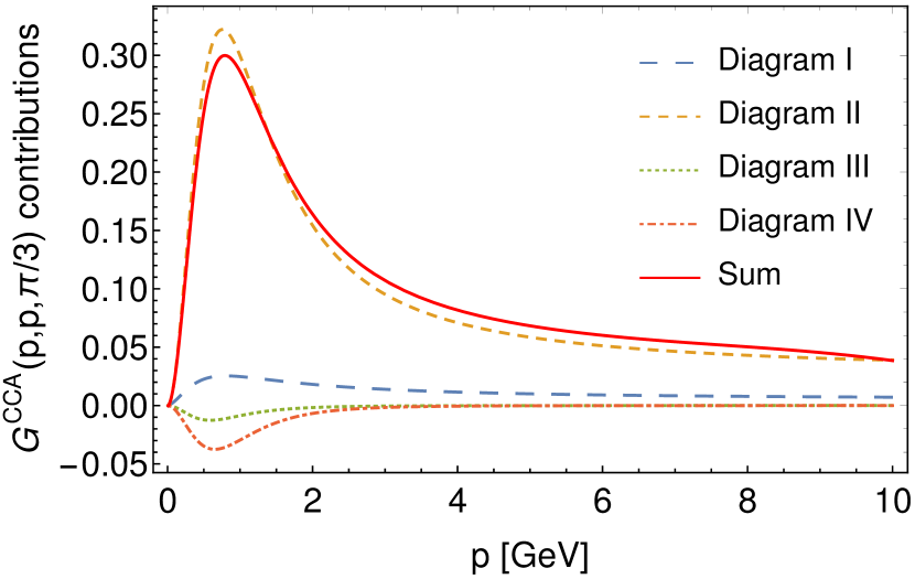
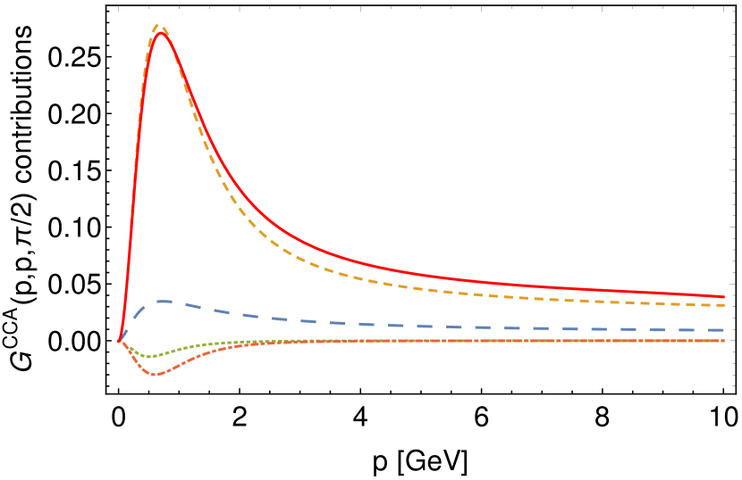
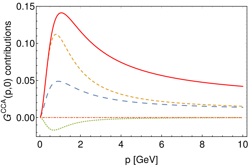
Figure 9: Contribution of each diagram to $G^{CCA}$ in three distinct configurations: the symmetric (top left), orthogonal (top right) and the soft gluon limit (bottom), using the gauge coupling described by eq. 38. Parameters, $\Lambda=0.70$ GeV and $g_{0}=2.15$, are chosen to minimize the relative error $\chi$ in the soft gluon limit. The convention of colors and line-styles in the orthogonal and soft configurations is the same as the symmetric case. The solid, red curve is the sum of all diagrams. The numbering of the diagrams is provided in fig. 1. Diagram (IV) refers to the full contribution $\frac{2g\gamma^{2}f^{ade}}{k^{2}+M^{2}}\Gamma_{\bar{c}^{b}c^{c}\varphi^{de}_{\mu}}(k,p,r)$.

VI Influence of the toy model on the UV behavior of the function $G^{CCA}$

As mentioned earlier, when comparing the UV tails of the dressing function $G^{CCA}$ obtained from the RGZ framework with other approaches, cf. figs. 4 and 8, we observe differences. Particularly striking is the observation in the case of SU(3), where a simultaneous comparison between the RGZ, the CF model and DSE results reveals a convergence in the tails from the latter approaches, starting from $p=4$ GeV onwards. In contrast, the UV tails of the curves from the RGZ framework decrease more rapidly. It is legitimate then to ask for the potential causes of this discrepancy in the UV. In this section we explore the extent to which this difference may derive from the toy model of the RG flow, as presented in eq. 38, and its associated parameters $\Lambda$ and $g_{0}$.

With that purpose we compare in fig. 10 the running of the gauge coupling employed for the CF prediction of $G^{CCA}$ at one-loop order in figs. 4 and 8 , denoted as $g_{\text{CF}}(\mu)$, with the running of the gauge coupling from eq. 38, $g_{\text{toy}}(\mu)$, with parameters $\Lambda$ and $g_{0}$, obtained from the fits for the gauge groups SU(2) and SU(3). We observe that $g_{\text{CF}}(\mu)$ and $g_{\text{toy}}(\mu)$ differ at all scales and, although the difference tends to diminish at high momenta, it is not negligible in the UV region.

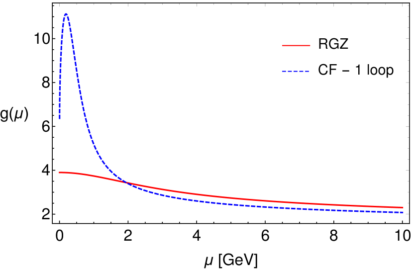
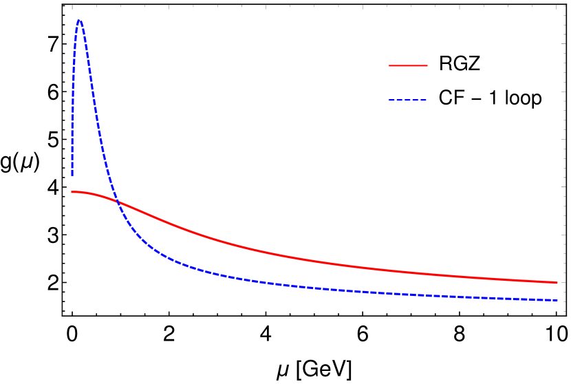
Figure 10: The running coupling $g_{\text{toy}}$ and $g_{\text{CF}}$ for the SU(2) (left) and SU(3) (right) gauge groups. As for the toy model, the values of the parameters are $\Lambda=2.4,$ GeV, $g_{0}=3.9$ and $\Lambda=0.70$ GeV, $g_{0}=2.15$, for SU(2) and SU(3), respectively.

An interesting analysis involves assessing how the differences among the UV tails of $G^{CCA}$ vary when we minimize the discrepancy between $g_{\text{CF}}(\mu)$ and $g_{\text{toy}}(\mu)$ in the UV domain. For this purpose, it is convenient to introduce the quantity $\chi_{g,UV}$, as a way to estimate that discrepancy:

$$\chi_{g,UV}^{2}\equiv\sum_{p_{i}=6\ \text{GeV}}^{{p_{i}=10\ \text{GeV}}}\Bigg{(}\frac{g_{\text{toy}}(p_{i})-g_{\text{CF}}(p_{i})}{g_{\text{CF}}(p_{i})}\Bigg{)}^{2}.$$ (40)

To carry out the summation we used uniform steps of length $\Delta p=p_{n+1}-p_{n}=0.5$ GeV. The parameters that minimize $\chi_{g,UV}$ are $\Lambda=1.05$ GeV, $g_{0}=6.75$ for the SU(2) gauge group and $\Lambda=0.90$ GeV, $g_{0}=4.85$ for SU(3). These parameters lead to an excellent agreement between $g_{\text{toy}}(\mu)$ and $g_{\text{CF}}(\mu)$ in the UV, as is illustrated in fig. 11 (black curve). Unfortunately, these values do not feature good compatibility with the lattice data of $G^{CCA}$.

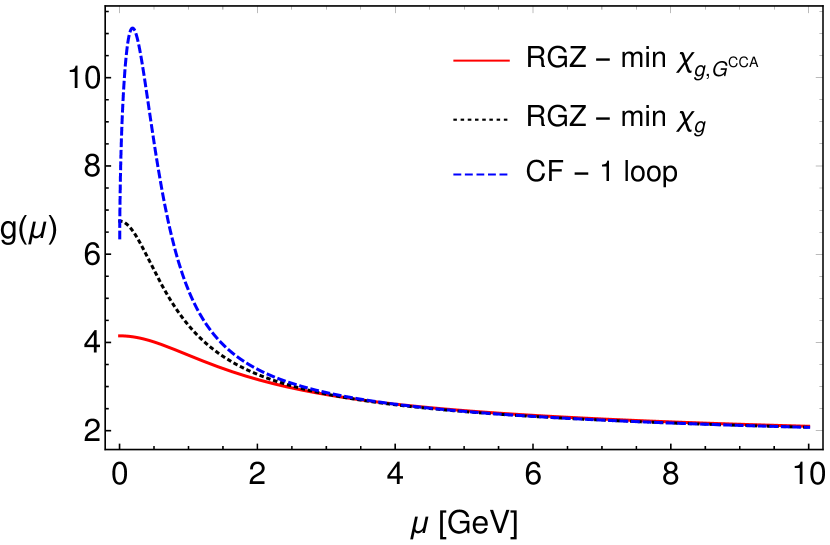
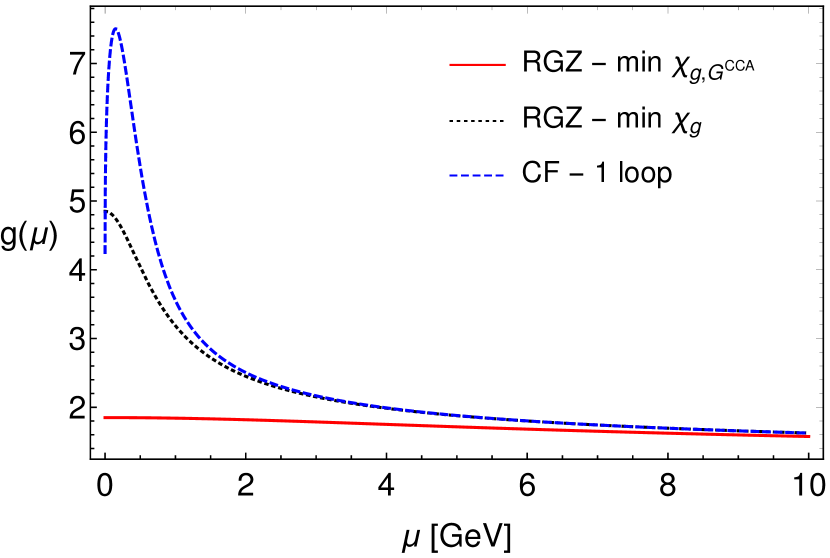
Figure 11: The running coupling $g_{\text{toy}}$ and $g_{\text{CF}}$ for the SU(2) (left) and SU(3) (right) gauge groups. The black curve corresponds to the parameters that minimize $\chi_{g,UV}^{2}$. These are $\Lambda=1.05$ GeV, $g_{0}=6.75$ and $\Lambda=0.90$ GeV, $g_{0}=4.85$, for SU(2) and SU(3) respectively. The red curve corresponds to the parameters that minimize $\chi_{g,G^{CCA}}$. These are $\Lambda=1.65$ GeV, $g_{0}=4.15$ and $\Lambda=5.05$ GeV, $g_{0}=1.85$, for SU(2) and SU(3) respectively.

To assess the potential for enhancing agreement between the results from the CF model and DSE with the RGZ framework without significantly compromising the IR description of lattice data, we introduce the following collective error

$$\chi_{g,G^{CCA}}^{2}=\frac{1}{2}\Big{(}\chi_{g,UV}^{2}+\chi_{G^{CCA}}^{2}\Big{)},$$ (41)

where $\chi_{G^{CCA}}$ is defined according to eq. 39 and eq. 37 for the SU(2) and SU(3) gauge groups, respectively. The quantity $\chi_{g,G^{CCA}}$ takes into account both the discrepancy between $g_{\text{CF}}(\mu)$ and $g_{\text{toy}}(\mu)$ in the UV as well as the discrepancy between the dressing function $G^{CCA}$ from the RGZ theory and the corresponding lattice data.

The parameters $\Lambda$ and $g_{0}$, derived from minimizing $\chi_{g,G^{CCA}}$, would in principle generate a gauge coupling $g_{\text{toy}}(\mu)$ that balances both the UV alignment with $g_{\text{CF}}(\mu)$ and the consistency with lattice data across all momentum scales. Such running coupling is also depicted in fig. 11 (red curve). In the case of the SU(2) gauge group, we notice an enhancement in the agreement in the UV region between RGZ and CF/DSE. Notably, this improvement does not imply a significant deterioration in the IR description. This is evident when comparing fig. 12 with fig. 4.

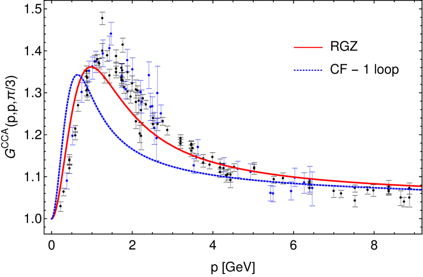
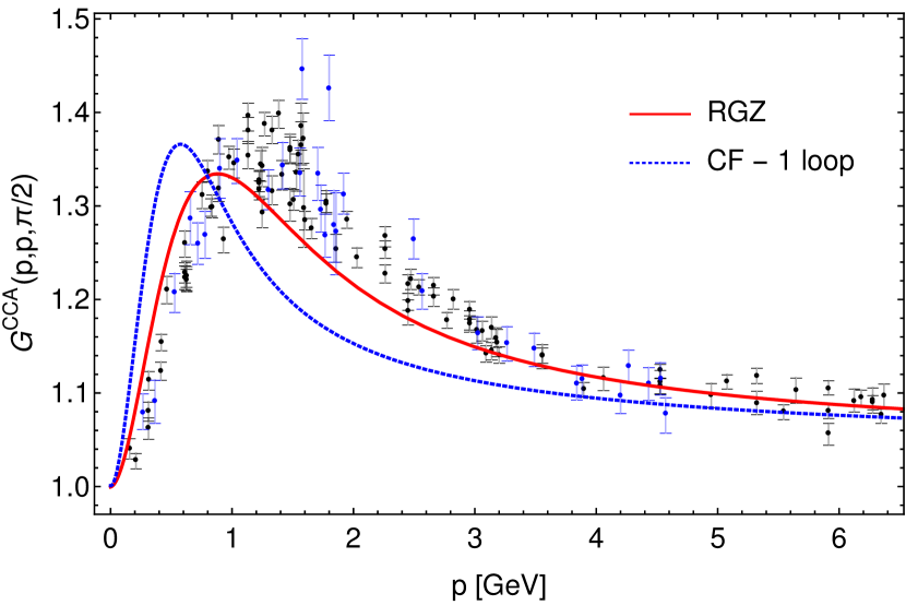
Figure 12: The scalar function $G^{CCA}$ as a function of the antighost external momentum in three distinct configurations: the symmetric (top left), orthogonal (top right) and the soft gluon limit (bottom) in the case of the SU(2) theory. The gauge coupling is described by the toy model of eq. 38 with parameters that minimize $\chi_{g,G^{CCA}}$, $\Lambda=1.65$ GeV and $g_{0}=4.15$.

In the case of SU(3), the minimization of $\chi_{G^{CCA}}$ leads to a running of the gauge coupling which is essentially constant. This is consistent with the plots of figs. 4 and 8, where a fixed value of $g$ was capable of describing the lattice data for the entirety range of momentum. However, the aforementioned running does not reduce the disagreement between the results from the CF model and DSE with the RGZ framework outcomes in the UV, being the quality of the fits similar to the ones presented in figs. 4 and 8. This is reasonable, since we are essentially neglecting the dependence of $g$ with the scale. Still, the results for SU(3) should be taken with care due to the dispersion of lattice data in the soft gluon limit and the lack of data in alternative kinematic setups.

We can conclude that the specific toy model we employed has an impact on the differences between the RGZ framework and other approaches in the UV region. However, these discrepancies probably have other sources as well such as the neglect of the RG flow of the remaining parameters of the theory and the specific choice of the renormalization scheme.

VII Summary and final remarks

In this work we evaluated the one-loop ghost-antighost-gluon correlation function within the RGZ framework for an arbitrary kinematic configuration and investigated the role of the running coupling. We performed the calculation for the pure gauge theory in a four dimensional Euclidean spacetime. With the purpose of comparing with other approaches, we specifically focused on three distinct kinematic configurations: the symmetric and orthogonal configurations and the soft gluon limit.

This calculation is important since it serves as a benchmark to assess how well the RGZ framework describes the behavior of YM theory in the low momentum regime. In this sense this paper comes to complement previous investigations on the two-point functions at tree-level order Dudal et al. (2008, 2010) and the analysis of the ghost-gluon vertex in the case of the soft-gluon limit at one-loop order Mintz et al. (2018).

The only parameter of the theory we used to fit our results to the available lattice data for the ghost-antighost-gluon vertex was the gauge coupling. All the other parameters were extracted from refs. Cucchieri et al. (2012) and Oliveira and Silva (2012), where they were determined by fitting lattice results for the gluon propagator using the RGZ tree level expression. This choice reduces the number of free parameters to the minimum, making the present analysis a more strict test of the RGZ framework.

As already pointed out in Mintz et al. (2018), as for the soft gluon limit the results are compatible with lattice simulations for both SU(2) Cucchieri et al. (2008); Maas (2020) and SU(3) Ilgenfritz et al. (2007) by simply considering a constant value of the gauge coupling, i.e. independent of the momentum scale. However, this is not the case of the symmetric and orthogonal configurations, where the renormalization group effects seem to be significant. Indeed, when introducing a toy model for the running of the gauge coupling, our outcomes are quantitatively compatible with available lattice data.

Our results also display qualitative agreement with other continuum approaches, specifically the dynamical DSE solutions in two different truncation schemes Aguilar et al. (2019) and the RG-improved CF model Pelaez et al. (2013); Barrios et al. (2020). Additionally, we show that quantitative differences between the RGZ results and alternative continuum approaches in the UV region can be accounted for by the particularities of the model for the RG flow of the gauge coupling.

Overall, these results support the RGZ theory as a valid description of the infrared YM dynamics. There are several ways, nevertheless, in which the present analysis can be improved. A fully dynamical calculation of the two-point functions of the RGZ framework, most likely in an infrared safe scheme, would allow us to determine the running parameters of the theory by fitting the two-point functions to lattice data. Another potential study concerning this correlation function could investigate its dependence on the gauge parameter within the context of linear covariant gauges, utilizing the BRST invariant version of the RGZ action Capri et al. (2016c).

Appendix A Relevant Feynman rules (Landau gauge)

Given its many fields and interactions, the RGZ theory has a large number of propagators and vertices. However, for the calculation of the ghost-gluon vertex at one-loop level (and in the Landau gauge), only a few of them are required. The Feynman rules corresponding to these propagators and vertices are shown below.

A.1 Tree-level propagators

In order to calculate the ghost-antighost-gluon 3-point function in the Refined Gribov-Zwanziger theory, only a subset of the propagators of the theory are needed. These are

$$\langle A^{a}_{\mu}(p)A^{b}_{\nu}(-p)\rangle = \delta^{ab}\left[\frac{p^{2}+M^{2}}{p^{4}+(m^{2}+M^{2})p^{2}+m^{2}M^{2}+2Ng^{2}\gamma^{4}}P^{\perp}_{\mu\nu}(p)\right]\equiv\delta^{ab}P^{\perp}_{\mu\nu}(p)D_{AA}(p)$$ (42)

$$\langle A_{\mu}^{a}(p)\varphi_{\nu}^{bc}(-p)\rangle = \frac{-ig\gamma^{2}f^{abc}}{p^{4}+p^{2}(m^{2}+M^{2})+m^{2}M^{2}+2Ng^{2}\gamma^{4}}P^{\perp}_{\mu\nu}(p)$$ (43)

$$\langle A_{\mu}^{a}(p)\bar{\varphi}_{\nu}^{bc}(-p)\rangle = \frac{-ig\gamma^{2}f^{abc}}{p^{4}+p^{2}(m^{2}+M^{2})+m^{2}M^{2}+2Ng^{2}\gamma^{4}}P^{\perp}_{\mu\nu}(p)=\langle A_{\mu}^{a}(p)\varphi_{\nu}^{bc}(-p)\rangle$$ (44)

$$\langle\bar{c}^{a}(p)c^{b}(-p)\rangle = \frac{1}{p^{2}}\delta^{ab}\equiv\delta^{ab}D_{\bar{c}c}(p)\;$$ (45)

where

$$P^{\perp}_{\mu\nu}(p)=\delta_{\mu\nu}-\frac{p_{\mu}p_{\nu}}{p^{2}}$$ (46)

is the transverse projector, such that $p_{\mu}P^{\perp}_{\mu\nu}(p)=p_{\nu}P^{\perp}_{\mu\nu}(p)=0$.

It is often convenient to write the $D_{AA}$ form factor as a sum of massive propagators, i.e.,

$$D_{AA}(p^{2}) = \frac{p^{2}+M^{2}}{(p^{2}+m^{2})(p^{2}+M^{2})+\lambda^{4}}\equiv\frac{R_{+}}{p^{2}+a_{+}^{2}}+\frac{R_{-}}{p^{2}+a_{-}^{2}},$$ (47)

with

$$a_{+}^{2}=\frac{m^{2}+M^{2}+\sqrt{(m^{2}-M^{2})^{2}-4\lambda^{4}}}{2},$$

$$a_{-}^{2}=\frac{m^{2}+M^{2}-\sqrt{(m^{2}-M^{2})^{2}-4\lambda^{4}}}{2},$$

$$R_{+}=\frac{m^{2}-M^{2}+\sqrt{(m^{2}-M^{2})^{2}-4\lambda^{4}}}{2\sqrt{(m^{2}-M^{2})^{2}-4\lambda^{4}}},$$

$$R_{-}=\frac{-m^{2}+M^{2}-\sqrt{(m^{2}-M^{2})^{2}-4\lambda^{4}}}{2\sqrt{(m^{2}-M^{2})^{2}-4\lambda^{4}}}=1-R_{+},$$ (48)

with $\lambda^{4}=2Ng^{2}\gamma^{4}$.

Note that either the poles $a_{+}$ and $a_{-}$ are complex, or the residues $R_{+}$ and $R_{-}$ have opposite signs (so that one of them is negative). This property can be directly related to positivity violation of the gluon propagator in the RGZ theory.

A.2 Tree-level vertices

The only vertices needed for the computation of the ghost-antighost-gluon at one-loop in the RGZ theory are

$${}^{\rm tree}[\Gamma_{AAA}(k,p,q)]^{abc}_{\mu\nu\rho} = -\left.\frac{\delta^{3}S_{\rm tree}}{\delta A_{\mu}^{a}(k)\delta A_{\nu}^{b}(p)\delta A_{\rho}^{c}(q)}\right|_{\Phi=0}=igf^{abc}\left[(k_{\nu}-q_{\nu})\delta_{\rho\mu}+(p_{\rho}-k_{\rho})\delta_{\mu\nu}+(q_{\mu}-p_{\mu})\delta_{\nu\rho}\right]\,,$$

$${}^{\rm tree}[\Gamma_{A\bar{c}c}(k,p,q)]^{abc}_{\mu} = -\left.\frac{\delta^{3}S_{\rm tree}}{\delta A_{\mu}^{a}(k)\delta\bar{c}^{b}(p)\delta c^{c}(q)}\right|_{\Phi=0}=-igf^{abc}p_{\mu}\,,$$

$${}^{\rm tree}[\Gamma_{A\bar{\varphi}\varphi}(k,p,q)]^{abcde}_{\mu\nu\rho} = -\left.\frac{\delta^{3}S_{\rm tree}}{\delta A_{\rho}^{a}(k)\delta\bar{\varphi}_{\mu}^{bc}(p)\delta\varphi_{\nu}^{de}(q)}\right|_{\Phi=0}=-igf^{abd}\delta^{ce}\delta_{\nu\rho}p_{\mu}\,.$$

Note that, for higher orders in the perturbative expansion, or for a general linear covariant gauge, or for other correlation functions, extra correlators and vertices will be needed.

Appendix B On the relation between connected and 1PI correlation functions in the presence of mixed propagators

Let us denote the generating functional of connected correlation functions as $W[\vec{J}]$, where $J_{i}$ are external sources associated with the different elementary fields, and let $\Gamma[\vec{\phi}]$ be the quantum action, that is, the generating functional of 1PI correlation functions. Using this notation, we start from the well-known relation

$$\left.\frac{\delta^{2}\Gamma[\vec{\phi}]}{\delta\phi_{j}\delta\phi_{\ell}}\right|_{\vec{\phi}=\vec{\Phi}[\vec{J}]}\frac{\delta^{2}W[\vec{J}]}{\delta J_{\ell}\delta J_{k}}=-\delta_{jk}$$ (50)

Taking a further derivative with respect to the source $J_{i}$, one finds

$$\frac{\delta^{3}W[\vec{J}]}{\delta J_{i}\delta J_{p}\delta J_{k}} = -\frac{\delta^{2}W[\vec{J}]}{\delta J_{p}\delta J_{j}}\left(\left.\frac{\delta^{3}\Gamma[\vec{\phi}]}{\delta\phi_{j}\delta\phi_{\ell}\delta\phi_{m}}\right|_{\vec{\phi}=\vec{\Phi}[\vec{J}]}\right)\frac{\delta^{2}W[\vec{J}]}{\delta J_{i}\delta J_{m}}\frac{\delta^{2}W[\vec{J}]}{\delta J_{\ell}\delta J_{k}}.$$ (51)

For the present calculation of the ghost-antighost-gluon vertex, we are specifically interested in the choice

$$i = A_{\mu}^{e}(k)$$

$$p = \bar{c}^{a}(p)$$

$$k = c^{b}(q).$$ (52)

Since there are no mixed propagators involving the Faddeev-Popov ghosts $c$ and $\bar{c}$, the only nonvanishing contributions are such that $j=c$ and $\ell=\bar{c}$. Therefore, running the remaining sum for $m=A,\varphi,\bar{\varphi}$, we have

$$\frac{\delta^{3}W[\vec{J}]}{\delta J_{A}\delta J_{\bar{c}}\delta J_{c}} = -\frac{\delta^{2}W[\vec{J}]}{\delta J_{c}\delta J_{\bar{c}}}\left\{\left(\left.\frac{\delta^{3}\Gamma[\vec{\phi}]}{\delta c\,\delta{\bar{c}}\,\delta A}\right|_{\vec{\varphi}=\vec{\Phi}[\vec{J}]}\right)\frac{\delta^{2}W[\vec{J}]}{\delta J_{A}\delta J_{A}}+\right.$$ (53)

$$+\left.\left(\left.\frac{\delta^{3}\Gamma[\vec{\phi}]}{\delta c\,\delta\,{\bar{c}}\,\delta\varphi}\right|_{\vec{\varphi}=\vec{\Phi}[\vec{J}]}\right)\frac{\delta^{2}W[\vec{J}]}{\delta J_{A}\delta J_{\varphi}}+\right.\left.\left(\left.\frac{\delta^{3}\Gamma[\vec{\phi}]}{\delta c\,\delta\,{\bar{c}}\,\delta\bar{\varphi}}\right|_{\vec{\varphi}=\vec{\Phi}[\vec{J}]}\right)\frac{\delta^{2}W[\vec{J}]}{\delta J_{A}\delta J_{\bar{\varphi}}}\right\}\frac{\delta^{2}W[\vec{J}]}{\delta J_{\bar{c}}\delta J_{c}},$$

which, at the one-loop level, can be written as

$$\left\langle{\bar{c}^{a}(p)\,c^{b}(q)\,A_{\mu}^{c}(k)}\right\rangle=D_{\bar{c}c}(p)D_{\bar{c}c}(q)D_{AA}(k)P_{\mu\nu}(k)\left\{\frac{\delta^{3}\Gamma}{\delta c^{a}(-p)\delta\bar{c}^{b}(-q)\delta A_{\nu}^{c}(-k)}+\frac{2g\gamma^{2}f^{cde}}{k^{2}+M^{2}}\frac{\delta^{3}\Gamma}{\delta c^{a}(-p)\delta\bar{c}^{b}(-q)\delta\varphi_{\nu}^{de}(-k)}\right\},$$

where we used the fact that the correlation functions obey $\left\langle{A\varphi}\right\rangle=\left\langle{A\bar{\varphi}}\right\rangle$, and also $\delta^{3}\Gamma/\delta c\delta\bar{c}\delta\varphi=\delta^{3}\Gamma/\delta c\delta\bar{c}\delta\bar{\varphi}$.

In a shorthand notation, one can conveniently write

$$\frac{\left\langle{A\,\bar{c}\,c}\right\rangle_{c}}{(\left\langle{\bar{c}\,c}\right\rangle_{c})^{2}\left\langle{AA}\right\rangle_{c}}=\Gamma_{A\,\bar{c}\,c}+\frac{\left\langle{A\,\varphi}\right\rangle_{c}}{\left\langle{A\,A}\right\rangle_{c}}\Gamma_{\bar{c}\,c\,\varphi}+\frac{\left\langle{A\,\bar{\varphi}}\right\rangle_{c}}{\left\langle{A\,A}\right\rangle_{c}}\Gamma_{\bar{c}\,c\,\bar{\varphi}}.$$ (55)

Therefore, besides the contribution $\Gamma_{A\bar{c}c}$, that would be present at pure Yang-Mills, there are also contributions from 1PI functions involving the auxiliary fields $\varphi$ and $\bar{\varphi}$, as well as the respective mixed propagators. Such contributions can be thought as momentum-dependent contributions to the ghost-gluon vertex, which are present starting from the tree level of the RGZ action.

Appendix C Analytic expression for the ghost-gluon vertex in the soft-gluon limit

In the soft-gluon limit (i.e., when the gluon momentum $k\rightarrow 0$), the expression (20) for the ghost-gluon vertex is relatively simpler than in a general kinematic regime. Given the absence of IR-divergences, the soft-gluon limit for the ghost-gluon vertex reads

$$\Gamma_{A^{a}_{\mu}\bar{C}^{b}C^{c}}(0,p,-p)=-igf^{abc}p_{\mu}B_{1}(0,p).$$ (56)

The scalar function $B_{1}(0,p)$ has been calculated (with a slightly different notation) to one-loop order in Mintz et al. (2018). The result can be written as

$$B_{1}(0,p) = 1+\frac{Ng^{2}}{2}\left[R_{+}J(a_{+};p)+R_{-}J(a_{-};p)\right]-Ng^{2}\left[R_{+}^{2}K(a_{+},a_{+};p)+R_{-}^{2}K(a_{-},a_{-};p)+2R_{+}R_{-}K(a_{+},a_{-};p)\right]$$ (57)

$$+\frac{Ng^{2}}{2}\frac{Ng^{2}\gamma^{4}}{(a_{+}^{2}-a_{-}^{2})^{2}}\left[K(a_{+},a_{+};p)+K(a_{-},a_{-};p)-2K(a_{+},a_{-};p)\right],$$

where the poles $a_{\pm}$ and residues $R_{\pm}$ of the tree-level gluon propagator are given by eq. (48), and the scalar functions $J$ and $K$ above are given by

$$J(m_{1};p) = \frac{1}{64\pi^{2}}\times\frac{2m_{1}^{2}p^{2}(p^{2}+m_{1}^{2})+p^{6}\log\left(1+\frac{m_{1}^{2}}{p^{2}}\right)-(3p^{2}+2m_{1}^{2})m_{1}^{4}\log\left(1+\frac{p^{2}}{m_{1}^{2}}\right)}{m_{1}^{2}p^{4}},$$ (58)

$$K(m_{1},m_{2};p) = \frac{1}{256\pi^{2}}\frac{1}{m_{1}^{2}m_{2}^{2}p^{4}(m_{1}^{2}-m_{2}^{2})}\bigg{\{}2m_{1}^{2}m_{2}^{6}p^{2}-2m_{1}^{6}m_{2}^{2}p^{2}+3m_{1}^{2}m_{2}^{4}p^{4}-3m_{1}^{4}m_{2}^{2}p^{4}+$$ (59)

$$\hskip 14.22636pt+\left.2m_{1}^{8}m_{2}^{2}\log\left(1+\frac{p^{2}}{m_{1}^{2}}\right)-2m_{1}^{2}m_{2}^{8}\log\left(1+\frac{p^{2}}{m_{2}^{2}}\right)+4m_{1}^{6}m_{2}^{2}p^{2}\log\left(1+\frac{p^{2}}{m_{1}^{2}}\right)-\right.$$

$$\hskip 17.07182pt\left.-4m_{1}^{2}m_{2}^{6}p^{2}\log\left(1+\frac{p^{2}}{m_{2}^{2}}\right)+4m_{1}^{2}m_{2}^{2}p^{6}\log\left(\frac{p^{2}+m_{2}^{2}}{p^{2}+m_{1}^{2}}\right)+\right.$$

$$\hskip 19.91684pt\left.+2m_{1}^{2}p^{8}\log\left(1+\frac{m_{2}^{2}}{p^{2}}\right)-2m_{2}^{2}p^{8}\log\left(1+\frac{m_{1}^{2}}{p^{2}}\right)\right\},$$

as for $m_{1}\neq m_{2}$, and

$$K(m,m;p)=\frac{-6p^{2}m^{6}-5p^{4}m^{4}-2p^{6}m^{2}+\left(8p^{2}m^{6}+6m^{8}\right)\log\left(1+\frac{p^{2}}{m^{2}}\right)+2p^{8}\log\left(1+\frac{m^{2}}{p^{2}}\right)}{256\pi^{2}p^{4}m^{4}}.$$ (60)

References

- Mintz et al. (2018) B. W. Mintz, L. F. Palhares, S. P. Sorella, and A. D. Pereira, Phys. Rev. D 97, 034020 (2018), arXiv:1712.09633 [hep-th] .
- Fodor and Hoelbling (2012) Z. Fodor and C. Hoelbling, Rev. Mod. Phys. 84, 449 (2012), arXiv:1203.4789 [hep-lat] .
- Durr et al. (2008) S. Durr et al. (BMW), Science 322, 1224 (2008), arXiv:0906.3599 [hep-lat] .
- Borsanyi et al. (2021) S. Borsanyi et al., Nature 593, 51 (2021), arXiv:2002.12347 [hep-lat] .
- Borsanyi et al. (2015) S. Borsanyi et al. (BMW), Science 347, 1452 (2015), arXiv:1406.4088 [hep-lat] .
- Bashir et al. (2012) A. Bashir, L. Chang, I. C. Cloet, B. El-Bennich, Y.-X. Liu, C. D. Roberts, and P. C. Tandy, Commun. Theor. Phys. 58, 79 (2012), arXiv:1201.3366 [nucl-th] .
- Aguilar et al. (2016) A. C. Aguilar, D. Binosi, and J. Papavassiliou, Front. Phys.(Beijing) 11, 111203 (2016), arXiv:1511.08361 [hep-ph] .
- Aguilar et al. (2023) A. C. Aguilar, F. De Soto, M. N. Ferreira, J. Papavassiliou, F. Pinto-Gómez, C. D. Roberts, and J. Rodríguez-Quintero, Phys. Lett. B 841, 137906 (2023), arXiv:2211.12594 [hep-ph] .
- Aguilar et al. (2022) A. C. Aguilar, M. N. Ferreira, and J. Papavassiliou, Phys. Rev. D 105, 014030 (2022), arXiv:2111.09431 [hep-ph] .
- Aguilar et al. (2021a) A. C. Aguilar, C. O. Ambrósio, F. De Soto, M. N. Ferreira, B. M. Oliveira, J. Papavassiliou, and J. Rodríguez-Quintero, Phys. Rev. D 104, 054028 (2021a), arXiv:2107.00768 [hep-ph] .
- Aguilar et al. (2021b) A. C. Aguilar, F. De Soto, M. N. Ferreira, J. Papavassiliou, and J. Rodríguez-Quintero, Phys. Lett. B 818, 136352 (2021b), arXiv:2102.04959 [hep-ph] .
- Huber et al. (2021) M. Q. Huber, C. S. Fischer, and H. Sanchis-Alepuz, Eur. Phys. J. C 81, 1083 (2021), [Erratum: Eur.Phys.J.C 82, 38 (2022)], arXiv:2110.09180 [hep-ph] .
- Fischer and Huber (2020) C. S. Fischer and M. Q. Huber, Phys. Rev. D 102, 094005 (2020), arXiv:2007.11505 [hep-ph] .
- Huber (2020) M. Q. Huber, Phys. Rev. D 101, 114009 (2020), arXiv:2003.13703 [hep-ph] .
- Aguilar et al. (2019) A. C. Aguilar, M. N. Ferreira, C. T. Figueiredo, and J. Papavassiliou, Phys. Rev. D 99, 034026 (2019), arXiv:1811.08961 [hep-ph] .
- Berges et al. (2002) J. Berges, N. Tetradis, and C. Wetterich, Phys. Rept. 363, 223 (2002), arXiv:hep-ph/0005122 [hep-ph] .
- Pawlowski (2007) J. M. Pawlowski, Annals Phys. 322, 2831 (2007), arXiv:hep-th/0512261 [hep-th] .
- Corell et al. (2018) L. Corell, A. K. Cyrol, M. Mitter, J. M. Pawlowski, and N. Strodthoff, SciPost Phys. 5, 066 (2018), arXiv:1803.10092 [hep-ph] .
- Cyrol et al. (2016) A. K. Cyrol, L. Fister, M. Mitter, J. M. Pawlowski, and N. Strodthoff, Phys. Rev. D 94, 054005 (2016), arXiv:1605.01856 [hep-ph] .
- Fischer et al. (2009) C. S. Fischer, A. Maas, and J. M. Pawlowski, Annals Phys. 324, 2408 (2009), arXiv:0810.1987 [hep-ph] .
- Dupuis et al. (2021) N. Dupuis, L. Canet, A. Eichhorn, W. Metzner, J. M. Pawlowski, M. Tissier, and N. Wschebor, Phys. Rept. 910, 1 (2021), arXiv:2006.04853 [cond-mat.stat-mech] .
- Nambu and Jona-Lasinio (1961) Y. Nambu and G. Jona-Lasinio, Phys. Rev. 122, 345 (1961).
- Klevansky (1992) S. P. Klevansky, Rev. Mod. Phys. 64, 649 (1992).
- Gell-Mann and Levy (1960) M. Gell-Mann and M. Levy, Nuovo Cim. 16, 705 (1960).
- Fukushima (2004) K. Fukushima, Physics Letters B 591, 277 (2004), arXiv:hep-ph/0310121 .
- Schaefer et al. (2007) B.-J. Schaefer, J. M. Pawlowski, and J. Wambach, Phys. Rev. D76, 074023 (2007), arXiv:0704.3234 [hep-ph] .
- Tissier and Wschebor (2010) M. Tissier and N. Wschebor, Phys. Rev. D 82, 101701 (2010), arXiv:1004.1607 [hep-ph] .
- Tissier and Wschebor (2011) M. Tissier and N. Wschebor, Phys. Rev. D84, 045018 (2011), arXiv:1105.2475 [hep-th] .
- Pelaez et al. (2013) M. Pelaez, M. Tissier, and N. Wschebor, Phys. Rev. D88, 125003 (2013), arXiv:1310.2594 [hep-th] .
- Peláez et al. (2014) M. Peláez, M. Tissier, and N. Wschebor, Phys. Rev. D 90, 065031 (2014), arXiv:1407.2005 [hep-th] .
- Peláez et al. (2015) M. Peláez, M. Tissier, and N. Wschebor, Phys. Rev. D 92, 045012 (2015), arXiv:1504.05157 [hep-th] .
- Gracey et al. (2019) J. A. Gracey, M. Peláez, U. Reinosa, and M. Tissier, Phys. Rev. D 100, 034023 (2019), arXiv:1905.07262 [hep-th] .
- Peláez et al. (2021) M. Peláez, U. Reinosa, J. Serreau, M. Tissier, and N. Wschebor, Rept. Prog. Phys. 84, 124202 (2021), arXiv:2106.04526 [hep-th] .
- Figueroa and Peláez (2022) F. Figueroa and M. Peláez, Phys. Rev. D 105, 094005 (2022), arXiv:2110.09561 [hep-th] .
- Barrios et al. (2020) N. Barrios, M. Peláez, U. Reinosa, and N. Wschebor, Phys. Rev. D 102, 114016 (2020), arXiv:2009.00875 [hep-th] .
- Barrios et al. (2021) N. Barrios, J. A. Gracey, M. Peláez, and U. Reinosa, Phys. Rev. D 104, 094019 (2021), arXiv:2103.16218 [hep-th] .
- Barrios et al. (2022) N. Barrios, M. Peláez, and U. Reinosa, Phys. Rev. D 106, 114039 (2022), arXiv:2207.10704 [hep-ph] .
- Siringo (2023) F. Siringo, Phys. Rev. D 107, 016009 (2023), arXiv:2211.06448 [hep-ph] .
- Siringo and Comitini (2023) F. Siringo and G. Comitini, Phys. Rev. D 107, 096001 (2023), arXiv:2210.11541 [hep-th] .
- Comitini et al. (2021) G. Comitini, D. Rizzo, M. Battello, and F. Siringo, Phys. Rev. D 104, 074020 (2021), arXiv:2108.00417 [hep-th] .
- Comitini and Siringo (2020) G. Comitini and F. Siringo, Phys. Rev. D 102, 094002 (2020), arXiv:2007.04231 [hep-ph] .
- Siringo and Comitini (2018) F. Siringo and G. Comitini, Phys. Rev. D 98, 034023 (2018), arXiv:1806.08397 [hep-ph] .
- Dudal et al. (2008) D. Dudal, J. A. Gracey, S. P. Sorella, N. Vandersickel, and H. Verschelde, Phys. Rev. D78, 065047 (2008), arXiv:0806.4348 [hep-th] .
- Dudal et al. (2010) D. Dudal, O. Oliveira, and N. Vandersickel, Phys. Rev. D81, 074505 (2010), arXiv:1002.2374 [hep-lat] .
- Gribov (1978) V. N. Gribov, Nucl. Phys. B139, 1 (1978).
- Zwanziger (1989) D. Zwanziger, Nucl. Phys. B323, 513 (1989).
- Dudal et al. (2019) D. Dudal, C. P. Felix, L. F. Palhares, F. Rondeau, and D. Vercauteren, Eur. Phys. J. C 79, 731 (2019), arXiv:1901.11264 [hep-th] .
- Vandersickel and Zwanziger (2012) N. Vandersickel and D. Zwanziger, Phys. Rept. 520, 175 (2012), arXiv:1202.1491 [hep-th] .
- Vandersickel (2011) N. Vandersickel, A Study of the Gribov-Zwanziger action: from propagators to glueballs, Ph.D. thesis, Gent U. (2011), arXiv:1104.1315 [hep-th] .
- Sobreiro and Sorella (2005) R. F. Sobreiro and S. P. Sorella, in 13th Jorge Andre Swieca Summer School on Particle and Fields (2005) arXiv:hep-th/0504095 .
- Capri et al. (2016a) M. A. L. Capri, M. S. Guimaraes, I. Justo, L. F. Palhares, and S. P. Sorella, Eur. Phys. J. C 76, 141 (2016a), arXiv:1510.07886 [hep-th] .
- Capri et al. (2015) M. A. L. Capri, D. Dudal, D. Fiorentini, M. S. Guimaraes, I. F. Justo, A. D. Pereira, B. W. Mintz, L. F. Palhares, R. F. Sobreiro, and S. P. Sorella, Phys. Rev. D92, 045039 (2015), arXiv:1506.06995 [hep-th] .
- Capri et al. (2016b) M. A. L. Capri, D. Fiorentini, M. S. Guimaraes, B. W. Mintz, L. F. Palhares, S. P. Sorella, D. Dudal, I. F. Justo, A. D. Pereira, and R. F. Sobreiro, Phys. Rev. D93, 065019 (2016b), arXiv:1512.05833 [hep-th] .
- Capri et al. (2016c) M. A. L. Capri, D. Dudal, D. Fiorentini, M. S. Guimaraes, I. F. Justo, A. D. Pereira, B. W. Mintz, L. F. Palhares, R. F. Sobreiro, and S. P. Sorella, Phys. Rev. D94, 025035 (2016c), arXiv:1605.02610 [hep-th] .
- Capri et al. (2017) M. A. L. Capri, D. Dudal, A. D. Pereira, D. Fiorentini, M. S. Guimaraes, B. W. Mintz, L. F. Palhares, and S. P. Sorella, Phys. Rev. D95, 045011 (2017), arXiv:1611.10077 [hep-th] .
- Gracey (2012) J. A. Gracey, Phys. Rev. D86, 105029 (2012), arXiv:1210.5962 [hep-th] .
- Lavelle and McMullan (1997) M. Lavelle and D. McMullan, Phys. Rept. 279, 1 (1997), arXiv:hep-ph/9509344 [hep-ph] .
- Capri et al. (2016d) M. A. L. Capri, D. Fiorentini, M. S. Guimaraes, B. W. Mintz, L. F. Palhares, and S. P. Sorella, Phys. Rev. D94, 065009 (2016d), arXiv:1606.06601 [hep-th] .
- Binosi et al. (2009) D. Binosi, J. Collins, C. Kaufhold, and L. Theussl, Comput. Phys. Commun. 180, 1709 (2009), arXiv:0811.4113 [hep-ph] .
- Cucchieri et al. (2006) A. Cucchieri, A. Maas, and T. Mendes, Phys. Rev. D 74, 014503 (2006), arXiv:hep-lat/0605011 .
- Piguet and Sorella (1995) O. Piguet and S. P. Sorella, Lect. Notes Phys. Monogr. 28, 1 (1995).
- Taylor (1971) J. C. Taylor, Nucl. Phys. B 33, 436 (1971).
- Sjödahl (2013) M. Sjödahl, Eur. Phys. J. C 73, 2310 (2013), arXiv:1211.2099 [hep-ph] .
- Passarino and Veltman (1979) G. Passarino and M. J. G. Veltman, Nucl. Phys. B 160, 151 (1979).
- Smirnov and Chuharev (2020) A. V. Smirnov and F. S. Chuharev, Comput. Phys. Commun. 247, 106877 (2020), arXiv:1901.07808 [hep-ph] .
- Martin (2003) S. P. Martin, Phys. Rev. D 68, 075002 (2003), arXiv:hep-ph/0307101 .
- Cucchieri et al. (2012) A. Cucchieri, D. Dudal, T. Mendes, and N. Vandersickel, Phys. Rev. D85, 094513 (2012), arXiv:1111.2327 [hep-lat] .
- Oliveira and Silva (2012) O. Oliveira and P. J. Silva, Phys. Rev. D86, 114513 (2012), arXiv:1207.3029 [hep-lat] .
- Cucchieri et al. (2008) A. Cucchieri, A. Maas, and T. Mendes, Phys. Rev. D77, 094510 (2008), arXiv:0803.1798 [hep-lat] .
- Maas (2020) A. Maas, SciPost Phys. 8, 071 (2020), arXiv:1907.10435 [hep-lat] .
- Ilgenfritz et al. (2007) E. M. Ilgenfritz, M. Muller-Preussker, A. Sternbeck, A. Schiller, and I. L. Bogolubsky, Braz. J. Phys. 37, 193 (2007), arXiv:hep-lat/0609043 [hep-lat] .
- (72) A. Rohatg, “Webplotdigitizer (version 4.3, july 2020),” https://automeris.io/WebPlotDigitizer.