Evaluation of block encoding for sparse matrix inversion using QSVT

Abstract

Three block encoding methods are evaluated for solving linear systems of equations using QSVT (Quantum Singular Value Transformation). These are arcsin, fable and prepare-select. The performance of the encoders is evaluated using a suite of 30 test cases including 1D, 2D and 3D Laplacians and 2D CFD matrices. A subset of cases is used to characterise how the degree of the polynomial approximation to $1/x$ influences the performance of QSVT. The results are used to guide the evaluation of QSVT as the linear solver in hybrid non-linear pressure correction and coupled implicit CFD solvers. The performance of QSVT is shown to be resilient to polynomial approximation errors. For both the pressure correction and coupled solvers, error tolerances of $10^{-2}$ are more than sufficient in most cases and in some cases $10^{-1}$ is sufficient. The pressure correction solver also allows subnormalised condition numbers, $\kappa_{s}$, as low as half of the theoretical values to be used. This resilience reduces the number of phase factors needed and, in turn, reduces the time to generate the factors and emulate QSVT. prepare-select encoding relies on a unitary decomposition, e.g. Pauli strings, that has significant classical preprocessing costs. Both arcsin and fable have much lower costs, particularly for coupled solvers. However, their subnormalisation factors, which are based on the rank of the matrix, can be many times higher than prepare-select leading to more phase factors being needed. For both the pressure correction and coupled CFD calculations, QSVT is more stable than previous HHL results due to polynomial approximation errors only affecting long wavelength CFD errors. Given that lowering $\kappa_{s}$ increases the success probability, optimising the performance of QSVT within a CFD code is a function of the number QSVT phase factors, the number of non-linear iterations and the number of shots. Although phase factor files can be reused, the time taken to generate them impedes scaling QSVT to larger test cases.

1 Introduction

With national quantum computing programmes, e.g. [1], increasing their focus on error-corrected devices, it is important for end-users to characterise and understand the likely performance of universal quantum algorithms. Previous work [2, 3] emulated the performance of the HHL (Harrow-Hassidim-Lloyd) algorithm [4] for two classes of Computational Fluid Dynamics (CFD) solver. Both involve the solution of a sequence of linear systems that dominate the run-time of classical solvers and are the most likely candidates for quantum advantage. With the appropriate number of eigenvalue qubits, HHL was shown to reproduce the classical solutions. However, the decomposition of the CFD matrices into Linear Combinations of Unitaries (LCU) [5] based on tensor products of Pauli operators required classical preprocessing with high computational costs - much higher than the classical CFD code. The classical preprocessing costs were most significant for the implicit CFD solver which transfers all matrix solutions to the quantum computer, leaving only matrix assembly on the classical computer.

An alternative to Trotterisation [6] used in the HHL evaluations is qubitization [5, 7, 8, 9]. Here, the LCU is used to encode the CFD matrix, $A$, by loading the LCU coefficients into a prepare register and the unitaries into a separate select register. The benefit of qubitization is that it gives an exact encoding of the CFD matrix up to a scale factor, thus, avoiding the approximation errors of Trotterization [10]. Whilst qubitization can be used in Quantum Phase Estimation [7] and, hence, HHL, the additional qubits needed for the prepare register add a significant overhead.

Quantum Singular Value Transformation (QSVT) [11, 12, 13] directly applies a polynomial function to the encoded matrix. If a sufficiently good polynomial approximation of $1/x$ is used then QSVT can encode $A^{-1}$ to within a user-defined accuracy and condition number. The asymptotic query complexity of QSVT, $\mathcal{O}(\kappa\log(\kappa/\epsilon))$ is better than the computational complexity of HHL, $O(log(N)s^{2}\kappa^{2}/\epsilon)$. QSVT also has the advantage of needing a single additional qubit for the signal processing register.

Whilst QSVT performs well with prepare-select encoding, as will be shown, it does not address the explosion in the number unitaries for implicit CFD matrices and the resulting classical preprocessing costs. Direct encoding of a matrix uses a query oracle to load the entries in the matrix [14, 15, 9, 16, 17]. These have small classical preprocessing costs but encoding circuit depths can scale with $\mathcal{O}(MN)$ for an $M\times N$ matrix. The circuit depths can be significantly reduced for encoders that target matrices with specific structures [18, 19]. The fable scheme [20] provides a general algorithm for reducing circuit depth which relies on transformation and then cancellation of rotation gates. Matrices that have a pattern of repeated values can be efficiently loaded using oracles based on indexing the entries according to how many times they have been repeated [21].

This work examines three matrix encoding techniques within the framework of QSVT as the linear equation solver for a non-linear CFD solver. The first is an arcsin variant of the matrix query oracle that uses $\sin^{-1}$ rather than $\cos^{-1}$ based encoding. This only encodes the non-zero elements of the matrix. The second is the fable encoding [20] and the third is prepare-select encoding. Future work will consider encoding based on repeated values. In addition to the CFD matrices, the encoders are investigated using a range of 1D, 2D and 3D Laplacian operators. These give matrices with a range of condition numbers that are used to characterise the properties of the different encoders.

The work is presented as follows. The test cases and their condition numbers are presented first as an area of interest is how the subnormalisation of each encoder affects the effective condition number, $\kappa_{s}$, for the QSVT phase factors. The encoding techniques are then described and their high-level circuit costs are evaluated. Next the QSVT algorithm is described, including the subnormalisation of the encoded matrix and the calculation of the phase factors. The influence of the subnormalisation on the number of phase factors is assessed. The influence on the precision of the phase factors on the accuracy of the QSVT solution relative to the classical solution is evaluated for a subset of the matrices. Finally, results for QSVT as a linear solver within a non-linear CFD solver are presented and conclusions drawn. All circuit diagrams use big-endian ordering.

2 Test cases

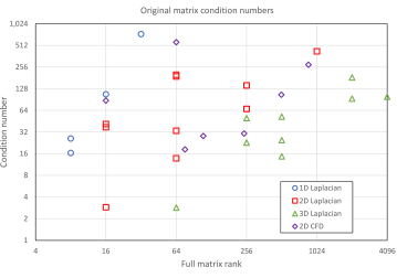
Figure 1: Condition numbers for the test matrices. Computed for original non-Hermitian matrices using GSL [22].

The focus of this evaluation is the solution of a linear system within an outer non-linear solver for applications such as Computational Fluid Dynamics (CFD). Three types of test case are used:

• Laplacian - 1, 2 and 3 dimensional Laplacian matrices generated using the L-QLES framework [23].

• Semi-Implicit CFD - 2D pressure correction matrices from the SIMPLE CFD cavity solver [2].

• Implicit CFD - 2D implicit matrices from the coupled CFD cavity solver [3].

Figure 1 shows the condition numbers for a range of matrices. The values plotted are listed in Table 3 in Appendix A. Whilst CFD matrices can be generated for a range of meshes, there is limited control over the resulting condition numbers. The Laplacian cases allow a wider range of condition numbers and matrix dimensions to be generated. This assists in the evaluation of matrix inversion using QSVT where the condition number is the primary factor in the number of phase factors needed.

In some of the small circuit illustrations in Section 3, the following matrix is used. This can be generated by the L-QLES framework but is degenerate and, hence, does not appear in Figure 1.

$$\frac{1}{2}\begin{pmatrix}[r]2&-1&0&0&0&0&0&-1\\ -1&2&-1&0&0&0&0&0\\ 0&-1&2&-1&0&0&0&0\\ 0&0&-1&2&-1&0&0&0\\ 0&0&0&-1&2&-1&0&0\\ 0&0&0&0&-1&2&-1&0\\ 0&0&0&0&0&-1&2&-1\\ -1&0&0&0&0&0&-1&2\\ \end{pmatrix}$$ (1)

3 Block encoding

Block encoding a matrix $A\in\mathbb{R}^{N\times N}$ with $N=2^{n}$ entails creating a unitary operator such that:

$$U_{A}=\begin{pmatrix}A/s&*\\ *&*\end{pmatrix}$$ (2)

where $s$ is the subnormalisation constant [15, 14]. The blocks denoted by $*$ are a result of the encoding and are effectively junk. Note that the encoding requires $||A||_{max}\leq 1$, any scaling to achieve this is independent of the subnormalisation factor. The application of the encoding unitary is such that:

$$\frac{A}{s}=(\bra{0^{m}}\otimes I_{n})U_{A}(\ket{0^{m}}\otimes I_{n})$$ (3)

Direct matrix encoders rely on a query-oracle, $O_{A}$ that returns the value for each entry $(i,j)$ in the matrix [14]:

$$O_{A}\ket{0}\ket{i}\ket{j}=\left(a_{ij}\ket{0}+\sqrt{1-|a_{ij}|^{2}}\ket{1}\right)\ket{i}\ket{j}$$ (4)

A circuit implementation of the block encoding unitary is shown in Figure 2 from [20].

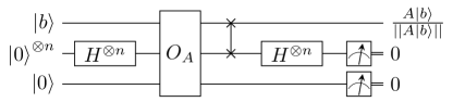
Figure 2: Schematic of block encoding circuit for $A/s$ from [20].

The query-oracle consists of row and column registers, each with $n=\log_{2}N$ qubits. Multi-controlled rotations are applied to an ancilla qubit. The multiplexing of controls are such that the correct entry $a_{ij}$ is loaded into the encoding block and $\sqrt{1-|a_{ij}|^{2}}$ is loaded into the junk block. Appendix B gives an explicit derivation of the block encoding of a 2x2 matrix. Figure 3 shows the full encoding circuit for a 4x4 matrix.

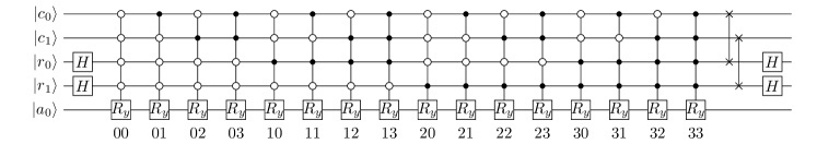
Figure 3: Block encoding circuit for a 4x4 matrix. Labels below the circuit indicate the row and column indices for the controlled rotations.

For this encoding circuit, the subnormalisation factor is $s=2^{n}$ and the probability of measuring all the ancilla qubits in the $\ket{0}$ state is [14]:

$$P(0^{n+1})=\frac{1}{s^{2}}||A\ket{b}||^{2}=\frac{1}{s^{2}}\bra{b}A^{\dagger}A\ket{b}$$ (5)

where $\ket{b}$ is the right hand side (RHS) state of the linear system $A\ket{x}=\ket{b}$ to be solved.

3.1 arcsin encoding

In order for the circuit in Figure 3 to correctly encode $A$, the rotation angles, $\theta$ must be set so that: $\theta_{ij}=2\cos^{-1}(a_{ij})$. For sparse matrices, this leads to a large circuit overhead as all the zero entries have rotation angles of $\pi$. Sparse matrix encoders can be thought of as equivalent to the Compressed Sparse Row (CSR) storage format. If $S_{r}$ is the maximum number of entries per row, the column oracle must convert the CSR index $0\leq s\leq S_{r}$ for each row into the corresponding column index. This generally requires an additional work register [14].

An alternative approach is presented in Appendix B where the rotation angles are calculated by $\theta_{ij}=2\sin^{-1}(a_{ij})$. This requires only the addition of a Pauli X gate on the ancilla rotation qubit at the end of the encoding circuit. This is equivalent to projecting the ancilla qubit into the $\ket{1}$ computational basis and the encoding oracle, with angles based on arcsin, becomes:

$$O_{A}\ket{0}\ket{i}\ket{j}=\left(\sqrt{1-|a_{ij}|^{2}}\ket{0}+a_{ij}\ket{1}\right)\ket{i}\ket{j}$$ (6)

There are now only as many multi-controlled rotations as there are non-zeros in the sparse matrix. However, the column indexing requires the same number of qubits in the column register.

3.1.1 Circuit trimming

arcsin encoding enables two options for reducing the depth of the encoding circuit. The first is to set rotation angles below a small threshold to zero, hence removing the corresponding operation from the ciruit. This is the same as setting small entries in the matrix to zero.

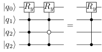
Figure 4: Coalescing multi-qubit controlled gates with a Hamming distance of 1 where the $R_{y}$ gates have the same rotation angle.

The second approach is to coalesce two multi-controlled operations which have the same rotation angle and where the two multiplexing strings are identical except for one qubit where they are bit-flipped. As shown in Figure 4 this is equivalent to the bit patterns for the multiplexing strings having a Hamming distance of 1. Since the multi-controlled rotations commute, the circuit can be reordered to find pairs that can be coalesced. The pairing can also applied recursively to pair previously coalesced operations.

Figure 5 shows a trimmed encoding circuit for the matrix in Equation 1. For example, on the second row of the matrix, the entries 1,0 are 1,2 are both equal and 1 bit flip apart. These are coalesced into the entry at 1,0. The subsequent rows, except the last, can be similarly trimmed. The current implementation always retains the operation with the lowest bit value. For this matrix, retaining entry 1,2 on row 2 and entry 3,2 on row 4 would allow further trimming.

More generally, approximations can be used to set values that are sufficiently close to have the same value. Caution is needed when approximating small values by zero. The value may be small because it makes a negligible contribution, or it may be zero because it represents a small scale in a multiscale discretisation.

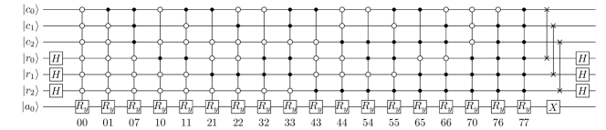
Figure 5: arcsin encoding circuit for 8x8 tri-diagonal matrix with coalesence of equal valued off-diagonal rotations on rows 1 to 6.

An advantage of the arcsin encoding is that trimming operations involve a direct correlation between the matrix entries and the rotation angles. Whilst setting matrix entries to zero or equal to others may assist fable and prepare-select encoding, their routes to circuit trimming involved derived quantities. More importantly, the changes to the matrix are known a priori and some of the effects may be able to be mitigated. For example, matrices resulting from a finite volume discretisation have a conservation property where the sum of the entries on a row is zero. Where matrix entries have been modified to reduce the circuit depth, additional changes can be made to recover the conservation property.

3.2 fable encoding

The fable method [20] is derived from the matrix query-oracle in Equation 4 and illusrated in Figure 3. The key insight in fable is to re-express the multi-controlled rotations as an interleaving sequence of uncontrolled rotations and CNOT gates in Gray code ordering. Further, if $\bm{\theta}$ is the $N$ dimensional vector of rotation angles used in $Q_{A}$, and $\bm{\hat{\theta}}$ the angles for the uncontrolled rotations in Gray code order, Then the angles are related by:

$$\bm{\theta}=2^{n}H^{\otimes 2n}P_{G}\bm{\hat{\theta}}$$ (7)

Where $H$ is the Hadamard gate and $P_{G}$ is the permutation matrix that transforms binary ordering to Gray code ordering. Equation 7 can be rewritten as:

$$\bm{\hat{\theta}}=\frac{1}{2^{n}}P_{G}^{\dagger}H^{\otimes 2n}\bm{\theta}$$ (8)

Since the inverse mapping $P_{G}^{\dagger}$ can be easily computed, the angles $\bm{\hat{\theta}}$ can be directly evaluated.

The premise of fable is that the solution of Equation 8 leads to a large number of angles that are zero or close to zero. Removing all angles with $\hat{\theta_{j}}\leq\delta_{c}$ leads to a block encoding error [20]:

$$||A-s\hat{A}||_{2}\leq N^{3}\delta_{c}+\mathcal{O}(\delta_{c}^{3})$$ (9)

where $\hat{A}$ is the encoding from Equation 3 with $U_{A}$ based on the thresholding of small angles.

Each rotation gate that is removed brings two CNOT gates together. Where there are sequences of zero-valued rotations, the resulting string of CNOTS may enable cancellation of pairs that operate on the same qubits. See Section B of [20]. Figure 6 shows the fable circuit for the same 8x8 tridiagonal matrix as shown in Figure 5.

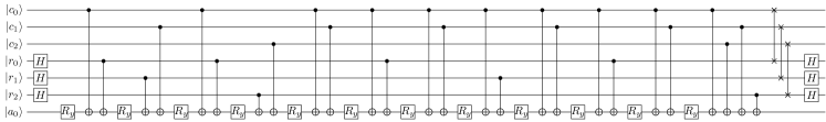
Figure 6: fable encoding circuit for 8x8 tri-diagonal matrix.

Note that the 8x8 matrix used in the figures has entries of 1 along the diagonal and -0.5 along the off diagonals, resulting in 52 of the 64 values of $\bm{\hat{\theta}}$ being zero, without the need for thresholding small values. When the number of zeros in $\bm{\hat{\theta}}$ is small, the conversion from multi-controlled rotations to uncontrolled rotations and CNOT gates may have benefits when the circuit is transpiled to native gates.

3.3 prepare-select encoding

prepare-select encoding follows from expressing the matrix to be encoded as a Linear Combination of Unitaries (LCU) [5, 8, 24, 25, 7, 9]:

$$A_{H}=\sum_{i=0}^{M-1}\alpha_{i}U_{i}$$ (10)

Where $M$ is the number of entries in the LCU and $A_{H}$ is bipartite Hermitian matrix with $A$ in the top right block and $A^{\dagger}$ in the bottom left block. If $A$ is already Hermitian, $A_{H}=A$. Typically, each unitary is a product of Pauli matrices. prepare-select encoding requires $\alpha_{i}>0$ which can be achieved by taking the signs of any negative coefficients into the corresponding unitary $U_{i}$. The resulting encoding unitary is:

$$U_{A}=(P^{\dagger}\otimes I^{n})S(P\otimes I^{n})$$ (11)

The prepare operator, $P$, is defined by its action of the $\ket{0}$ state:

$$P\ket{0}=\sum_{i=0}^{M-1}\sqrt{\frac{\alpha_{i}}{s}}\ket{i}$$ (12)

where $s=\norm{\alpha}_{1}=\sum_{i=0}^{M-1}|\alpha_{i}|$ is the $L_{1}$ norm of the coefficients and is the subnormalisation constant. Essentially, $P$ is a state loader for the coefficients $\sqrt{\frac{\alpha_{i}}{s}}$. In this work, the a binary tree data loader is used [26, 27]. In gereral, the number of unitaries, $M$, in the LCU is not a power of 2 and the vector of coefficients passed to the state loader must be padded with zeros.

The select operator, $S$ is:

$$S=\sum_{i=0}^{M-1}\ket{i}\bra{i}\otimes U_{i}$$ (13)

Figure 7 shows the prepare-select circuit for encoding a 4x4 matrix with 4 entries in its LCU.

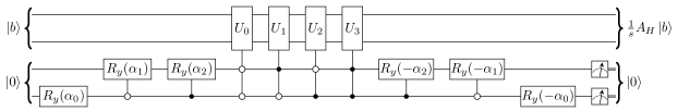
Figure 7: Circuit for encoding a 4x4 matrix using prepare-select.

3.4 Comparison of encoding techniques

Performing a like-with-like comparison of the three encoding schemes is not straightforward as they result in different styles of circuits. Hence, only an order of magnitude analysis is undertaken. For both arcsin and fable encoding, the number of rotation gates is used. This ignores the fact that arcsin uses multi-controlled rotations and fable uses single qubit rotations. The number of CNOT gates in fable circuit is also ignored. For prepare-select, the number of terms in the LCU is used. This is multiplied by a factor of 3 as the Prepare circuit, its adjoint and the Select circuit have the same number of operations. Hadamard and swap gates that scale with the number of qubits are not counted.

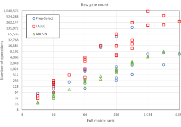
Figure 8: Number of encoding operations. Rotation gates for fable and arcsin encoding and number of unitaries in the LCU for prepare-select.

Figure 8 shows the operation counts for each of the cases in Figure 1. The plotted values are listed in Table 4 in Section A.2. By construction, the number of operations in the arcsin encoding scales with the number of non-zeros in the matrix. Most of the prepare-select cases have similar scaling except for those for the coupled CFD matrices which have close to $\mathcal{O}(N^{2})$ scaling. The fable results show the largest scatter.

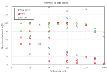
Figure 9: Normalised operation counts for the data in Figure 8.

An alternative view of the number of operations is shown in Figure 9. Here, the prepare-select and arcsin encodings are normalised by the number of non-zeros and the fable encoding by $N^{2}$. For the Laplacian cases, fable encoding is very effective on the larger cases - although the raw number of operations remains very high. The arcsin circuit trimming reduces the operation count for many but not all of the Laplacian cases. However, it is not as effective as fable at doing so. As with fable, there are Laplacian cases where prepare-select encoding uses only a small percentage of Pauli strings. There are also cases where the number of prepare-select operations far exceeds the number of non-zeros. Several of these are not shown in Figure 9 including all of the coupled CFD matrices. For the CFD matrices, the number of fable and arcsin operations are both close to 100%. By construction, they cannot be larger. As shown in Figure 9 this does not mean they have the same number of operations.

Applying the fable mapping, Equation 8, to the arcsin encoding is possible if all the zero angle rotations are included to enable the Gray coding step to be completed. This was tested and found to produce very similar operation counts to the fable scheme. Whether the initial vector of angles, $\bm{\theta}$, contained a large number of zeros or a large number angles equal to $\pi$, had only a small effect on the number of non-zero angles in the output vector $\bm{\hat{\theta}}$.

Demultiplexing the multiplexed rotations [28, 29] in the arcsin and prepare-select encoding increases the number of rotation gates by a factor of $\mathcal{O}(\log_{2}N)$. This has not been done as multiplexed operators are efficient to implement in emulation.

Since, without any approximations, arcsin and fable encoding result in the same unitary and have the same subnormalisation factor the following analysis will omit fable, as arcsin encoding is more efficient to emulate. The results labelled arcsin can also be read as being fable results.

4 Quantum Singular Value Transformation

Quantum Singuar Value Transformation (QSVT) derives from Quantum Signal Processing [11, 30, 12, 13] and applies a polynomial function $P$ to the encoded block in Equation 2:

$$\begin{pmatrix}A/s&*\\ *&*\end{pmatrix}\xmapsto{QSVT}\begin{pmatrix}P(A/s)&*\\ *&*\end{pmatrix}$$ (14)

The Polynomial is implemented by interleaving applications of $U_{A}$ and $U_{A}^{\dagger}$ with projector controlled phase shifts as shown in Figure 10. For an odd polynomial of degree $d$, the transformation is:

$$S_{\vec{\phi}}=\Pi_{\phi_{1}}U\left[\prod\limits_{k=1}^{(d-1)/2}\Pi_{\phi_{2k}}U_{A}^{\dagger}\Pi_{\phi_{2k+1}}U_{A}\right]$$ (15)

where $\Pi_{\phi}$ is a projector controlled phase shift operator: $\Pi_{\phi}=e^{i2\phi\Pi}$. The implementation of the desired polynomial transformation depends of the the phase factors, $\phi_{k}$ for $k={0,\ldots,d-1}$.

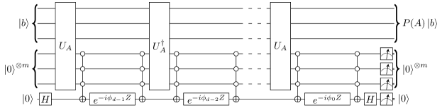
Figure 10: QSVT circuit for the transformation in Equation 15 for 8x8 matrix and a degree-d odd polynomial.

4.1 Subnormalisation

The subnormalisation constant, $s$ depends on the method of block encoding. For prepare-select, $s=\norm{\alpha}_{1}=\sum_{i=0}^{M-1}|\alpha_{i}|$ where $\alpha$ is the vector of coefficients in the LCU decomposition. For the query oracles, fable and arcsin encoding, $s=N$.

In addition, for query-oracless, it must also be ensured that $||A||_{max}\leq 1$. For solving linear systems, this is applied as an external scaling prior to QSVT:

$$\frac{A}{||A||_{max}}\ket{x}=\frac{1}{||A||_{max}}\ket{b}$$ (16)

Scaling both $A$ and $\ket{b}$ ensures that the solution to the original system is recovered.

When computing the phase factors for the matrix inversion it is the condition number $\kappa_{s}$ of $A/s$ that should be used. Due to the subnormalisation, if the encoded matrix is square, this gives:

$$\kappa_{s}=\frac{1}{|\lambda^{min}_{s}|}$$ (17)

where $\lambda^{min}_{s}$ is the smallest eigenvalue of $A/s$. If $A/s$ is not square, then $\lambda^{min}_{s}$ is the smallest singular value. Note that while $\lambda^{min}_{s}=\lambda^{min}/s$ this does not, in general, mean that $\kappa_{s}=s\kappa$. However, it does give:

$$\frac{\kappa_{s}}{s}=\frac{1}{|\lambda^{min}|}$$ (18)

For arcsin encoding, if $||A||_{max}<1$, it is beneficial to apply the scaling in Equation 16 as this increases $\lambda^{min}_{s}$ and reduces $\kappa_{s}$ since the subnormalisation constant is unchanged. For prepare-select encoding this is not needed as the scaling increases both the minimum eigenvalue and the LCU coefficients and does not affect the subnormalisation constant.

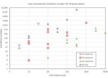
Figure 11: Condition numbers for subnormalised matrix using prepare-select encoding.

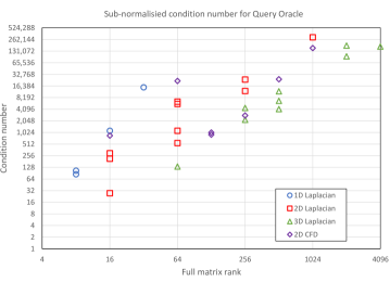
Figure 12: Condition numbers for subnormalised matrix using arcsin encoding.

Figure 11 shows the subnormalised condition numbers for all the test cases using prepare-select encoding. For the Laplacian and pressure correction CFD matrices the scaling relative to the original matrices is $\mathcal{O}(1)$. For the coupled CFD matrices the scaling is $\mathcal{O}(10)$ due to far greater number of unitaries in the LCU.

Figure 12 shows the subnormalised condition numbers using arcsin encoding. Here, the scaling is equal to the rank of the matrix. Note that this is not a direct scaling of the original condition number as $\kappa_{s}$ depends on $|\lambda^{min}_{s}|$. Note also that the ranks for coupled CFD matrices are for the encoded block for which the rank is a power of 2. The subnormalised condition numbers for both encoding methods are listed in Table 3 in Section A.1.

4.2 Scaling the QSVT solution

As with all QLES methods, the normalised solution state $\ket{\hat{x}}$ must be scaled to return the correct solution to the original matrix equation. As the matrix being scaled by subnormalisation factor, the polynomial being applied is also scaled. For the Dong et al. [13] Remez approximation used here, the polynomial being approximated is:

$$P(x)=\frac{1}{4\kappa_{s}x}$$ (19)

Hence, if QSVT has accurately implemented $P$, the state at the end of QSVT is:

$$\ket{0^{m+1}}\otimes\ket{\hat{b}}\xmapsto{QSVT}\ket{0^{m+1}}\otimes\frac{s}{4\kappa_{s}}A^{-1}\ket{\hat{b}}+\ket{\Phi^{\perp}}$$ (20)

Where $\ket{\Phi^{\perp}}$ is the orthogonal junk state. The expectation, $E$, of measuring all the $m+1$ flag qubits in the $\ket{0}$ state is:

$$E=\left(\frac{s}{4\kappa_{s}}\right)^{2}||A^{-1}||_{2}^{2}$$ (21)

And the post measurement state in the encoding qubits is:

$$\frac{1}{\sqrt{E}}\frac{s}{4\kappa_{s}}A^{-1}\ket{\hat{b}}=\frac{1}{\sqrt{E}}\frac{s}{4\kappa_{s}}\ket{\hat{x}}$$ (22)

If the normalised input state is $\ket{\hat{b}}=\ket{b}/||\bra{b}||_{2}$, the re-dimensionalised output state is:

$$\ket{x}=\frac{4\kappa_{s}}{s}\sqrt{E}||\ket{b}||_{2}\ket{\hat{x}}$$ (23)

Whilst the expectation Equation 21 has no explicit dependence on $\epsilon$, the analysis has not accounted for the degree to which $P$ approximates $A^{-1}$. This influence will be analysed Section 4.4.

4.3 Computing the phase factors

The phase factors are calculated via the Remez method [13, 31] using the open-sourced qsppack software package. Whilst the degree of the polynomial scales with $\mathcal{O}(\kappa\log(1/\epsilon))$, setting the value of the degree can involve some trial and error. Within the context of QLES, the required accuracy of solution state also has a bearing on the degree of the polynomial. To investigate this, a tridiagonal Toeplitz matrix is used:

$$T_{n}(a,b,c)=\begin{pmatrix}a&c&&&&&\\ b&a&c&&&&\\ &b&a&c&&&\\ &&\ddots&\ddots&\ddots&&\\ &&&&b&a&c\\ &&&&&b&a\\ \end{pmatrix}$$ (24)

For which, the eigenvalues are:

$$\lambda_{k}=a-2\sqrt{bc}\cos(\frac{k\pi}{n+1}),k=1,\ldots,n$$ (25)

Equation 25 enables a matrix with a specified condition number to be created. To make this easier, the settings $a=1$ and $b=c$ are used. Using prepare-select encoding, a 32x32 Toeplitz matrix with $\kappa=28.8$ gave a subnormalised matrix with $\kappa_{s}=49.98$. Using the error relative to the classical solution, qsppack was used to generate phase factors for $\kappa_{s}=50$ and $L_{\infty}$ errors of $10^{-1}$, $10^{-2}$ and $10^{-3}$. The degrees were adjusted to give approximately the same errors in the $L_{2}$ norms of QSVT solution of the Toeplitz matrix. The resulting degrees were 109, 229 and 359. For this analysis, the amplitudes of right hand side vector, $\ket{b}$ were set from: $b_{i}=16x_{i}^{3}-24x_{i}^{2}+9x_{i}$ for $i=0,N-1$ and $x_{i}=1/(N-1)$.

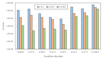
Figure 13: $L_{2}$ errors for range of Laplacians and qsppack $L_{\infty}$ error tolerances. All with $\kappa_{s}=50$ phase factors and prepare-select encoding.

$\kappa_{s}$	Case name	Case index
27.5	l2d_8x8_dddd	8
48.0	l3d_8x8x8_ddrrdd	19
51.3	l2d_8x8_ddrr	9
54.7	l2d_4x4_rrrr	7
62.3	l3d_4x8x8_dndddd	16
77.2	l2d_4x4_nnnn	6
100.5	l3d_4x8x8_dnrrdd	17

Table 1: Test cases order by subnormalised condition number using prepare-select encoding. Case index refers to position in Table 3.

Figure 13 shows the influence of qsppack $L_{\infty}$ tolerance on the Toeplitz matrix for the Laplacian cases listed in Table 1. All the solutions are calculated using the same expression for $\ket{b}$ as used in the Toeplitz calculations, and all were solved using prepare-select encoding. There is some variation in the $L_{2}$ error levels between the cases. As expected, the $L_{2}$ solver errors increase for the cases with higher condition numbers and the benefits of more accurate phase factors becomes more marginal. Further analysis using the RHS states generated by the L-QLES framework showed that the $L_{2}$ error levels are also influenced by the eigen spectrum of the input state which is dependent on the matrix.

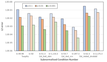
Figure 14: $L_{2}$ errors compared to classical solutions. Comparison of prepare-select (solid) and arcsin (hatched) encoding for Toeplitz, l2d_8x8_ddrr, l2d_4x4_rrrr and l3d_4x8x8_dndddd cases. The condition numbers are the subnormalised values for each encoding. Phase factors for $L_{\infty}=0.001$ and $\kappa_{s}>2000$ were not available.

Figure 14 compares the $L_{2}$ errors with prepare-select and arcsin encoding for the Toeplitz, l2d_4x4_nnnn, l2d_4x4_rrrr and l3d_4x8x8_dndddd cases. All the prepare-select cases use the $\kappa_{s}=50$ phase factors as used previously. For arcsin, the 32x32 Toeplitz matrix with $\kappa=2.125$ gives an encoded matrix with $\kappa_{s}=50$ allowing a direct comparison with prepare-select. For the larger condition numbers, the longer run times of qsppack make it impractical to optimise the degree of the polynomial approximation. For the arcsin cases, phase factors for subnormalised condition numbers 300, 1,000 and 2,500 were used. Whilst this does not give an exact back to back comparison, it is indicative of how QSVT would be used in practice. qsppack reliably generated all the phase factors used in this work with the largest set having 16,813 factors.

4.4 Success probability

Figure 15 shows the success probability of measuring the signal and encoding qubits in the $\ket{0}$ state as in Figure 10, using the same test cases as above. Apart from the Toeplitz matrix with prepare-select encoding, the two encoding methods have very similar success factors with small variations due to the different $L_{\infty}$ errors levels of polynomial approximations.

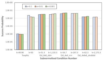
Figure 15: Success probabilities. Comparison of prepare-select (solid) and arcsin (hatched) encoding for Toeplitz, l2d_8x8_ddrr, l2d_4x4_rrrr and l3d_4x8x8_dndddd cases. The condition numbers are the subnormalised values for each encoding. Phase factors for $L_{\infty}=0.001$ and $\kappa>1000$ were not available.

Since the Toeplitz cases use different condition numbers to achieve the same $\kappa_{s}$, the subnormalisation constants for prepare-select and arcsin encoding are $s=3.34$ and $s=32$ respectively. From Equation 21, the scaling with $s^{2}$ results in the 2 orders of magnitude difference in the success probabilities. For the other cases Equation 18 shows that, as long as $\kappa_{s}$ is chosen according to Equation 17, the success probability is independent of the encoding method shown.

Measurement	Qubit	Expectation	Qubit	Expectation
order	order		order
$E_{0}$	9	9.583055e-01	16	6.105163e-02
$E_{1}$	10	8.883451e-01	9	1.000000e+00
$E_{2}$	11	9.170198e-01	10	1.000000e+00
$E_{3}$	12	9.430148e-01	11	1.000000e+00
$E_{4}$	13	9.522488e-01	12	1.000000e+00
$E_{5}$	14	9.626014e-01	13	1.000000e+00
$E_{6}$	15	9.754071e-01	14	1.000000e+00
$E_{7}$	16	9.275374e-02	15	1.000000e+00
E(Success)		6.105162e-02		6.105162e-02

Table 2: Influence of the measurement order on the expectation of success for the l3d_4x8x8_dnrrdd test case. Big endian ordering, qubit 16 = QSVT signal qubit.

An interesting observation on the expectations of the measurements is shown in Table 2. This is for the l3d_4x8x8_dnrrdd test case with prepare-select encoding, but the same observation is true for arcsin encoding. For this case, there are 9 qubits in the Select register, 7 qubits in the prepare register and one signal processing qubit. With big endian ordering, the default is to measure the qubits in ascending order, which measures the signal qubit last. The flag qubits used in the encoding have expectations close to one but not exactly one. If, instead, the signal qubit is measured first and is in the $\ket{0}$ state, then all the flag qubits are also projected onto the $\ket{0}$ state. At least, in the error-free simulations used herein. As expected, the overall success probability is independent of the measurement order.

5 Results

These results focus on the use of QSVT as the linear solver within an outer non-linear Computational Fluid Dynamics solver. Two types of linear system are considered. The first is the pressure-correction solver used within semi-implicit CFD schemes. The second is the coupled matrix from an implicit CFD solver. Both are applied to the 2-dimensional lid-driven cavity for which hybrid HHL solutions have been reported [2, 3]. The same hybrid methodology has been used in this work. Convergence plots show the change in the flow variables between the start and end of each linear QSVT solution. If the change is high, the non-linear set of equations are far from being satisfied. As the outer non-linear iterations proceed, the changes reduce towards zero at which point the non-linear solution has been found.

All calculations were run on an Intel^® Core^© i9 12900K 3.2GHz Alder Lake 16 core processor with 64GB of 3,200MHz DDR4 RAM.

5.1 Pressure correction equations

The smallest 2D pressure correction matrix is for a 5x5 CFD mesh that results in a 16x16 matrix. From Table 3, this has subnormalised condition numbers of 133 and 850 for prepare-select and arcsin encoding respectively.

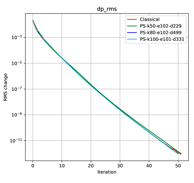
(a) prepare-select encoding

(b) arcsin encoding.

Figure 16: Convergence history of the pressure correction updates for the 16x16 pressure correction using QSVT. k is conditional number, e is precision (e.g. 102 = $10^{-2}$), d is the number of phase factors.

Figure 16(a) compares the classical solution with QSVT solutions for $\kappa_{s}=50,80,100$ phase factors using prepare-select encoding. Even with $\kappa_{s}=50$ and $\epsilon=0.01$, the QSVT convergence is almost identical to the classical one. These are well below the expected condition number of 133. Figure 16(b) performs the same comparison for arcsin encoding where the expected condition number is 850. Here, the $\kappa_{s}=1000,\epsilon=0.1$ and $\kappa_{s}=400,\epsilon=0.01$ phase factors match the classical solution and have approximately the same number of phase factors. Even the $\kappa_{s}=200$ solution is reasonable. Summed over all the non-linear iterations, it has a total of 107,835 phase rotations compared to 168,351 for $\kappa_{s}=1000$.

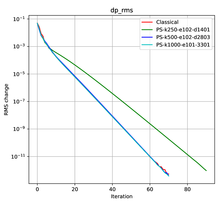
(a) prepare-select encoding

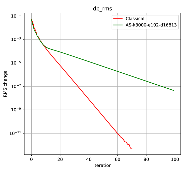
(b) arcsin encoding.

Figure 17: Convergence history of the pressure correction updates for the 64x64 pressure correction using QSVT. k is conditional number, e is precision (e.g. 102 = $10^{-2}$), d is the number of phase factors.

Figure 17 compares the encoding techniques on the 9x9 CFD mesh which has a 64x64 pressure correction matrix. From Table 3, this has subnormalised condition numbers of 1,186 and 22,063 for prepare-select and arcsin encoding respectively. The prepare-select results are similar to the results for the 16x16 matrix. For the arcsin results, the highest number of phase factors available was for $\kappa_{s}=3000,\epsilon=0.01$. It took qsppack 10.5 days to generate the 16,813 phase factors. Most of this was applying the Remez algorithm to construct the approximating polynomial [13]. The BFGS optimisation to get the phase factors took 5.5 hours, which could be reduced to less than an hour with Newton optimisation [31]. Assuming that phase factors for $\kappa_{s}=12000$ would be sufficient, the $\mathcal{O}(\kappa^{2})$ scaling of qsppack [13] means that it would take over 5 months to generate them.

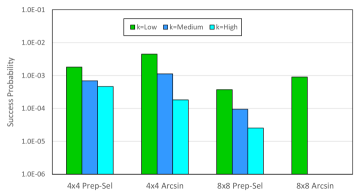
Figure 18: Success probabilities for pressure correction solver. Colours and order match Figure 16 and Figure 17.

The QSVT results match previous findings for the effect of precision on HHL [3]. The early iterations are dominated by high frequency error waves corresponding to the largest eigenvalues. These are accurately resolved by QSVT. However, these error waves are quickly eliminated and low frequency waves, associated with the smaller eigenvalues, become dominant. As with HHL, failure to model the effects of lowest eigenvalues leads to slow convergence rather than divergence.

Figure 18 shows the success probabilities for matrices sampled at 10 iterations from each of the above cases. The change in expectation with condition number is consistent with Equation 21. For the 4x4 case using arcsin encoding, there is an extra benefit of using $\kappa_{s}=200$ instead of $\kappa_{s}=1000$ as it gives a factor 25 increase in success probability.

5.2 Implicit coupled equations

The smallest 2D implicit matrix is for a 5x5 CFD mesh that results in a 76x76 matrix which is padded with an identity block to 128x128. From Table 3, this has subnormalised condition numbers of 331 and 900 for prepare-select and arcsin encoding respectively.

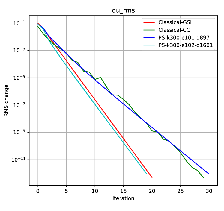
(a) prepare-select encoding

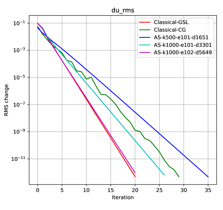
(b) arcsin encoding.

Figure 19: Convergence history of the velocity updates for the 76x76 implicit matrix using QSVT. k is conditional number, e is precision (e.g. 102 = $10^{-2}$), d is the number of phase factors.

Figure 19(a) compares the classical solution with QSVT solutions for $\kappa_{s}=300$ and $\epsilon=0.1,0.02$ phase factors using prepare-select encoding. There are two classical solutions included in the plots. The solution labelled ’GSL’ uses an exact solver [22] and the solution labelled ’CG’ uses an iterative conjugate gradient solver [32]. The lower precision QSVT solution matches the CG solution and the higher precision matches the GSL solution. The arcsin solutions in Figure 19(b) show the same behaviour. For the arcsin encoding, the pressure correction and implicit matrices have similar condition numbers, $\kappa_{s}$, of around 900. Whilst the pressure correction matrix can use phase factors for $\kappa_{s}=400$ with no discernible effect, the implicit matrix has a near doubling of the number of non-linear iterations if phase factors for $\kappa_{s}=500$ are used.

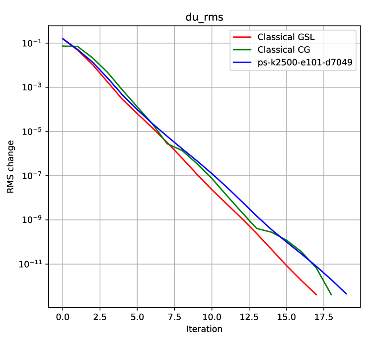
(a) prepare-select encoding

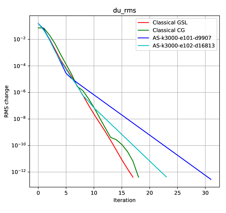
(b) arcsin encoding.

Figure 20: Convergence history of the velocity updates for the 244x244 implicit matrix using QSVT. Labelling as before.

Figure 20(a) compares the classical and QSVT coupled solutions for the 9x9 CFD mesh with prepare-select encoding, for which $\kappa_{s}=2,407$. Given the long run times for this case, see Section 5.2.1, only one QSVT calculation was performed with phase factors for $\kappa_{s}=2,500,\epsilon=0.1$. The QSVT solution matches the Classical conjugate gradient solution. Note that the CG and GSL classical solutions are more similar but the CG solver required a single SIMPLE iteration at the start to prevent it diverging. The QSVT solution did not need this. A further indication that QSVT may yield stability benefits. Figure 20(b) compares the classical and QSVT coupled solutions with arcsin encoding, for which $\kappa_{s}=2,824$. Due to the time taken by qsppack to generate phase factors only two QSVT solutions are available with $\kappa_{s}=3,000$ and $\epsilon=0.01,0.1$. These show the same trends as for the 5x5 coupled calculations.

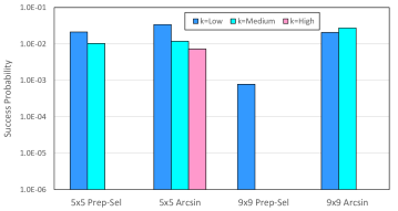
Figure 21: Success probabilities for implicit solver. Colours and order match Figure 19 and Figure 20.

Figure 21 shows the success probabilities for coupled QSVT solutions. The scaling with $\kappa_{s}$ shows the expected behaviour. Of note is that the coupled solver has higher success probabilities than the pressure correction solver. This is in part due to lower condition numbers, but also due to the fact that the pressure correction matrices have to be scaled down to achieve $|A|_{max}=1$ whereas the coupled matrices can be scaled up. These differences are included in the values in Table 3.

5.2.1 Computational considerations

For the prepare-select encoding of the 9x9 coupled case, the LCU contained 16,104 Pauli strings although the time to compute these was less than a minute. The main computational consideration was that the LCU resulted in the prepare register having 14 qubits compared to 8 in the equivalent row register. The prepare operations are the most time consuming to emulate and, even with the optimisations described in Section C.1, each phase factor step took 2.4s, compared to 0.01s for arcsin. For the prepare-select result in Figure 20(a) with 7,049 phase factors, each complete QSVT solve took just under 5 hours compared to less than 3 minutes for arcsin with 16,183 phase factors. Whilst classical emulation times should not be taken as indicative of the time on a physical quantum computer, the difference in the operational intensity of the two encoding methods is likely to have some relevance.

6 Conclusions

A sparse matrix query oracle using arcsin encoding generates circuits that scale with the number of non-zeros in the matrix. This has minimal classical preprocessing costs and addresses one of the major issues of prepare-select encoding based on Pauli strings - the classical preprocessing time to construct the LCU. The downside of the arcsin encoding is that the subnormalisation constant $s$ scales with the size of the matrix. For pressure correction based CFD solvers this leads to an $\mathcal{O}(n_{d}/N)$ overhead relative to prepare-select encoding, where $n_{d}$ is the number of diagonals in the matrix. However, for the implicit coupled CFD solver, the vastly increased number of Pauli strings in the LCU gives greater parity in the subnormalisation constants.

A key part of QSVT is setting $\kappa_{s}$ to accurately resolve the influence of the eigenvectors with the lowest eigenvalues. These are responsible for long-wavelength errors in the CFD flow field and setting $\kappa_{s}$ too low slows the rate of convergence but does not, generally, lead to divergence. Given that lowering $\kappa_{s}$ increases the success probability, optimising the performance of QSVT within a CFD code is a function of the number QSVT phase factors, the number of non-linear iterations and the number of shots.

The $L_{\infty}$ approximation errors in the QSVT phase factors has been found to less impactful than the condition number. Error tolerances of $10^{-2}$ were more than sufficient in most cases and in some cases $10^{-1}$ was sufficient. There are some indications that QSVT is more robust in the first iterations of an implicit solver that often require special treatment in classical solvers. However, the cases are orders of magnitude from industrial matrices results and these inferences must be treated with caution.

With the goal of minimising the time spent on a classical computer using hybrid implicit CFD solvers, arcsin encoding for the query-oracle has shown that QSVT can be an effective linear solver. However, the time taken to generate the QSVT phase factors remains a significant impediment to scaling QSVT to larger test cases. Unlike constructing a LCU, the calculation of each set of phase factors is a one-off calculation separate from the CFD solver. The unifying nature of QSVT means that a library of phase factors can be used to invert a wide range of matrix types.

7 Data availability

The L-QLES input files for the Laplacian test cases are available from https://github.com/rolls-royce/qc-cfd.

8 Acknowledgements

I would like to thank Christoph Sünderhauf of Riverlane for his guidance and many useful discussions on the implementation of QSVT. I would also like to thank Bjorn Berntson and Zal Nemeth of Riverlane for their help in choosing the input parameters for QSPPACK. I would also like to thank Jarrett Smalley and Tony Phipps of Rolls-Royce for their helpful comments on this work. This work would not have been possible without QSPPACK and I would like to thank Yulong Dong of UC Berkeley for his advice at the outset of this work.

The permission of Rolls-Royce to publish this work is gratefully acknowledged. This work was completed under funding received under the UK’s Commercialising Quantum Technologies Programme (Grant reference 10004857).

Appendix A Test case details

In the following tables, the naming convention for the Laplacian cases, those with ’l’ as the first character is: dimension_mesh_bcs. The input files for these cases are available at github.com/rolls-royce/qc-cfd. For CFD matrices labelled cavity-pc, the mesh dimensions are for the pressure correction mesh. For the cavity-cpl matrices, the mesh dimensions are for the nodal mesh. For example, cavity-pc-4x4 and cavity-cpl-5x5 are different solvers on the same mesh.

For the coupled CFD cases, the matrix dimension is that of the original CFD system. As described in [3], the matrix is padded with a diagonal block to give a dimension that is the next largest power of 2.

A.1 Condition numbers

Index	Case name	rank (A)	$\kappa$ (A)	$\kappa$ (AH)	$\kappa$ (PS)	$\kappa$ (QO)
1	l1d_8_dd	8	15.3	16.4	26.1	84.7
2	l1d_8_rr	8	25.3	26.0	41.8	105.1
3	l1d_16_dd	16	99.1	107.3	180.9	1,134.5
4	l1d_32_dd	32	698.3	735.8	1287.7	15,101.5
5	l2d_4x4_dddd	16	2.4	2.9	3.8	27.4
6	l2d_4x4_nnnn	16	25.7	41.3	77.2	213.8
7	l2d_4x4_rrrr	16	36.2	37.3	54.7	297.3
8	l2d_8x8_dddd	64	13.5	13.8	27.5	544.0
9	l2d_8x8_ddrr	64	33.1	33.3	51.3	1,133.3
10	l2d_8x8_nnnn	64	155.8	189.1	527.3	5,583.2
11	l2d_8x8_rrrr	64	199.5	200.4	346.9	6,416.1
12	l2d_16x16_dddd	256	62.0	67.0	196.7	12,151.6
13	l2d_16x16_ddrr	256	140.7	142.0	317.8	23,956.2
14	l2d_32x32_dddd	1,024	401.3	423.6	1,501.5	298,501.1
15	l3d_4x4x4_dndddd	64	3.2	5.5	5.9	113.2
16	l3d_4x8x8_dndddd	256	14.4	22.8	62.3	2,175.3
17	l3d_4x8x8_dnrrdd	256	32.6	50.0	100.5	4,405.3
18	l3d_8x8x8_dddddd	512	14.5	14.7	37.1	4,127.9
19	l3d_8x8x8_ddrrdd	512	24.6	24.7	48.0	6,752.8
20	l3d_8x8x8_dnrrdd	512	44.7	52.3	121.1	11,897.0
21	l3d_8x16x16_dndddd	2,048	62.4	93.1	422.8	95,420.9
22	l3d_8x16x16_dnrrdd	2,048	136.8	183.6	615.2	181,163.7
23	l3d_16x16x16_dddddd	4,096	82.7	98.1	301.7	171,397.3
24	cavity-pc-4x4	16	87.7	88.7	133.5	851.2
25	cavity-pc-8x8	64	567.3	568.3	1,186.2	22,063.6
26	cavity-cpl-5x5	76	18.3	20.9	331.4	900.3
27	cavity-cpl-6x6	109	28.2	28.2	583.4	1,021.1
28	cavity-cpl-9x9	244	30.5	72.8	2,407.4	2,823.5
29	cavity-cpl-13x13	508	105.7	205.9	11,707.9	24,374.5
30	cavity-cpl-17x17	868	275.5	483.8	-	156,973.6

Table 3: Full matrix rank and condition numbers $\kappa$ for each case. A = original non-Hermitian matrix, AH = symmetrised Hermitian matrix, PS = prepare-select encoding using AH, QO = Query Oracle (arcsin and fable) encoding using A.

Table 3 gives the condition numbers for all the cases used in this study. The condition numbers are computed using the GNU Scientific Library [22]. There are 4 columns of condition number:

• $\kappa$ (A) - the original non-Hermitian matrices.

• $\kappa$ (AH) - the symmetrised Hermitian matrices.

  $$AH=\begin{pmatrix}0&A\\ A^{\dagger}&0\end{pmatrix}$$ (26)

• $\kappa$ (PS) - the sub-normalised matrices using prepare-select encoding. The condition number for the 17x17 coupled matrix is absent as the time to compute the LCU was too excessive.

• $\kappa$ (QO) - the sub-normalised matrices using arcsin and fable encoding.

A.2 Operation counts

Index	Case name	rank (A)	#non-zeros (A)	prepare-select	fable	arcsin
1	l1d_8_dd	8	20	42	32	20
2	l1d_8_rr	8	22	57	42	18
3	l1d_16_dd	16	44	96	128	43
4	l1d_32_dd	32	92	216	512	88
5	l2d_4x4_dddd	16	32	60	64	32
6	l2d_4x4_nnnn	16	40	204	208	40
7	l2d_4x4_rrrr	16	76	195	166	53
8	l2d_8x8_dddd	64	208	288	1,024	208
9	l2d_8x8_ddrr	64	256	102	384	232
10	l2d_8x8_nnnn	64	232	864	3,328	232
11	l2d_8x8_rrrr	64	316	783	2,608	252
12	l2d_16x16_dddd	256	1,040	1,344	16,104	990
13	l2d_16x16_ddrr	256	1,152	360	5,632	1,013
14	l2d_32x32_dddd	1,024	4,624	6,141	188,825	4,384
15	l3d_4x4x4_dndddd	64	116	180	1,024	112
16	l3d_4x8x8_dndddd	256	724	816	16,332	686
17	l3d_4x8x8_dnrrdd	256	880	264	5,116	777
18	l3d_8x8x8_dddddd	512	1,808	1,629	31,919	1,808
19	l3d_8x8x8_ddrrdd	512	2,240	528	12,192	2,096
20	l3d_8x8x8_dnrrdd	512	2,288	540	20,477	2,288
21	l3d_8x16x16_dndddd	2,048	9,300	7,296	589,491	8,183
22	l3d_8x16x16_dnrrdd	2,048	10,336	1,704	198,452	8,588
23	l3d_16x16x16_dddddd	4,096	9,104	6,147	292,884	7,144
24	cavity-pc-4x4	16	62	189	256	62
25	cavity-pc-8x8	64	286	957	4,074	286
26	cavity-cpl-5x5	76	317	13,536	16,377	308
27	cavity-cpl-6x6	109	440	15,696	16,354	440
28	cavity-cpl-9x9	244	1,117	48,312	65,401	1,103
29	cavity-cpl-13x13	508	2,525	146,868	259,326	2,525
30	cavity-cpl-17x17	868	4,669	-	1,003,800	4,608

Table 4: Number of operations for each test case and encoding scheme.

In Table 4 the number of operations are counted as follows. For both arcsin and fable encoding, the number of rotation gates is used. This ignores the fact that arcsin uses multi-controlled rotations and fable uses single qubit rotations. The number of CNOT gates in fable circuit is also ignored. For prepare-select, the number of terms in the LCU is used. This is multiplied by a factor of 3 as the prepare circuit, its adjoint and the Select circuit have the same number of operations. Hadamard and swap gates that scale with the number of qubits are not counted.

Appendix B Encoding a 2x2 matrix encoding

This section shows the assembly of the query oracle encoding of a 2x2 matrix as this may be of interest to some readers. The encoding circuit is shown in Figure 22.

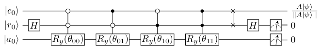
Figure 22: Circuit for full encoding of a 2x2 matrix using big-endian indexing.

Each of the controlled rotations in Figure 22 can be written as:

$$U_{ij}=I^{\otimes 3}+(R_{ij}-I)\otimes M_{i}\otimes M_{j}$$ (27)

Where $R_{ij}$ is shorthand for $R(\theta_{ij})$ and $i,j\in{0,1}$. The $M$ matrices are the single qubit measurement operators in the computational basis:

$$M_{0}=\ket{0}\bra{0}=\begin{pmatrix}1&0\\ 0&0\end{pmatrix}$$ (28)

$$M_{1}=\ket{1}\bra{1}=\begin{pmatrix}0&0\\ 0&1\end{pmatrix}$$ (29)

Expanding for $U_{00}$ gives:

$$U_{00}=\begin{pmatrix}1&0&0&0&0&0&0&0\\ 0&1&0&0&0&0&0&0\\ 0&0&1&0&0&0&0&0\\ 0&0&0&1&0&0&0&0\\ 0&0&0&0&1&0&0&0\\ 0&0&0&0&0&1&0&0\\ 0&0&0&0&0&0&1&0\\ 0&0&0&0&0&0&0&0\\ \end{pmatrix}+\begin{pmatrix}c_{00}-1&-s_{00}\\ s_{00}&c_{00}-1\end{pmatrix}\otimes\begin{pmatrix}1&0&0&0\\ 0&0&0&0\\ 0&0&0&0\\ 0&0&0&0\\ \end{pmatrix}$$ (30)

Giving

$$U_{00}=\begin{pmatrix}c_{00}&0&0&0&-s_{00}&0&0&0\\ 0&1&0&0&0&0&0&0\\ 0&0&1&0&0&0&0&0\\ 0&0&0&1&0&0&0&0\\ s_{00}&0&0&0&c_{00}&0&0&0\\ 0&0&0&0&0&1&0&0\\ 0&0&0&0&0&0&1&0\\ 0&0&0&0&0&0&0&0\\ \end{pmatrix}$$ (31)

Performing the matrix products of the controlled rotations gives

$$U_{A}=\prod_{i,j=0}^{1}U_{i,j}=\begin{pmatrix}c_{00}&0&0&0&-s_{00}&0&0&0\\ 0&c_{01}&0&0&0&-s_{01}&0&0\\ 0&0&c_{10}&0&0&0&-s_{10}&0\\ 0&0&0&c_{11}&0&0&0&-s_{1,1}\\ s_{00}&0&0&0&c_{00}&0&0&0\\ 0&s_{01}&0&0&0&c_{01}&0&0\\ 0&0&s_{10}&0&0&0&c_{10}&0\\ 0&0&0&s_{11}&0&0&0&c_{1,1}\\ \end{pmatrix}=\begin{pmatrix}C&-S\\ S&C\end{pmatrix}$$ (32)

Where $c_{ij}=\cos\frac{\theta_{ij}}{2}$ and $s_{ij}=\sin\frac{\theta_{ij}}{2}$. Note that the controlled rotation operators commute and, hence, the ordering of the products in Equation 32 is not important. The final matrix in Equation 32 contains the 4x4 cosine and sine blocks. The following matrices will also be expressed in terms of 4x4 blocks.

The Hadamard operator on the row qubit is

$$I\otimes H\otimes I=\frac{1}{\sqrt{2}}\begin{pmatrix}1&0&1&0&0&0&0&0\\ 0&1&0&1&0&0&0&0\\ 1&0&-1&0&0&0&0&0\\ 0&1&0&-1&0&0&0&0\\ 0&0&0&0&1&0&1&0\\ 0&0&0&0&0&1&0&1\\ 0&0&0&0&1&0&-1&0\\ 0&0&0&0&0&1&0&-1\\ \end{pmatrix}=\begin{pmatrix}\tilde{H}&0\\ 0&\tilde{H}\end{pmatrix}$$ (33)

The swap operator on the row and column qubits is:

$$I\otimes SWAP=\begin{pmatrix}1&0&0&0&0&0&0&0\\ 0&0&1&0&0&0&0&0\\ 0&1&0&0&0&0&0&0\\ 0&0&0&1&0&0&0&0\\ 0&0&0&0&1&0&0&0\\ 0&0&0&0&0&0&1&0\\ 0&0&0&0&0&1&0&0\\ 0&0&0&0&0&0&0&1\\ \end{pmatrix}=\begin{pmatrix}S_{W}&0\\ 0&S_{W}\end{pmatrix}$$ (34)

Using the 4x4 block representations, accumulating the circuit operators gives:

$$\begin{array}[]{rcl}\left(I\otimes H\otimes I\right)\left(I\otimes SWAP\right)U_{A}\left(I\otimes H\otimes I\right)&=&\begin{pmatrix}\tilde{H}&0\\ 0&\tilde{H}\end{pmatrix}\begin{pmatrix}S_{W}&0\\ 0&S_{W}\end{pmatrix}\begin{pmatrix}C&-S\\ S&C\end{pmatrix}\begin{pmatrix}\tilde{H}&0\\ 0&\tilde{H}\end{pmatrix}\\[20.0pt] &=&\begin{pmatrix}\tilde{H}S_{W}C\tilde{H}&-\tilde{H}S_{W}S\tilde{H}\\ \tilde{H}S_{W}S\tilde{H}&\tilde{H}S_{W}C\tilde{H}\end{pmatrix}\end{array}$$ (35)

Evaluating the upper left 4x4 block gives:

$$\begin{array}[]{rcl}\tilde{H}S_{W}C\tilde{H}&=&\frac{1}{2}\begin{pmatrix}1&0&1&0\\ 0&1&0&1\\ 1&0&-1&0\\ 0&1&0&-1\\ \end{pmatrix}\begin{pmatrix}1&0&0&0\\ 0&0&1&0\\ 0&1&0&0\\ 0&0&0&1\\ \end{pmatrix}\begin{pmatrix}c_{00}&0&0&0\\ 0&c_{01}&0&0\\ 0&0&c_{10}&0\\ 0&0&0&c_{11}\\ \end{pmatrix}\begin{pmatrix}1&0&1&0\\ 0&1&0&1\\ 1&0&-1&0\\ 0&1&0&-1\\ \end{pmatrix}\\[20.0pt] &=&\frac{1}{2}\par\begin{pmatrix}1&0&1&0\\ 0&1&0&1\\ 1&0&-1&0\\ 0&1&0&-1\\ \end{pmatrix}\begin{pmatrix}1&0&0&0\\ 0&0&1&0\\ 0&1&0&0\\ 0&0&0&1\\ \end{pmatrix}\begin{pmatrix}c_{00}&0&c_{00}&0\\ 0&c_{01}&0&c_{01}\\ c_{10}&0&-c_{10}&0\\ 0&c_{11}&0&-c_{11}\\ \end{pmatrix}\\[20.0pt] &=&\frac{1}{2}\par\begin{pmatrix}1&0&1&0\\ 0&1&0&1\\ 1&0&-1&0\\ 0&1&0&-1\\ \end{pmatrix}\begin{pmatrix}c_{00}&0&c_{00}&0\\ c_{10}&0&-c_{10}&0\\ 0&c_{01}&0&c_{01}\\ 0&c_{11}&0&-c_{11}\\ \end{pmatrix}\\[20.0pt] &=&\frac{1}{2}\par\begin{pmatrix}c_{00}&c_{01}&c_{00}&c_{01}\\ c_{10}&c_{11}&-c_{10}&-c_{11}\\ c_{00}&-c_{01}&c_{00}&-c_{01}\\ c_{10}&-c_{11}&-c_{10}&c_{11}\\ \end{pmatrix}\end{array}$$ (36)

Setting $\theta_{ij}=2\cos^{-1}(a_{ij})$, the upper left 2x2 block contains the original matrix with a subnormalisation factor of 2.

B.1 Arcsin based encoding

If instead of $I\otimes SWAP$ in Equation 34, $X\otimes SWAP$ is used, see Figure 23, then Equation 35 becomes:

$$\begin{array}[]{rcl}\left(I\otimes H\otimes I\right)\left(X\otimes SWAP\right)U_{A}\left(I\otimes H\otimes I\right)&=&\begin{pmatrix}\tilde{H}&0\\ 0&\tilde{H}\end{pmatrix}\begin{pmatrix}0&S_{W}\\ S_{W}&0\end{pmatrix}\begin{pmatrix}C&-S\\ S&C\end{pmatrix}\begin{pmatrix}\tilde{H}&0\\ 0&\tilde{H}\end{pmatrix}\\[20.0pt] &=&\begin{pmatrix}\tilde{H}S_{W}S\tilde{H}&\tilde{H}S_{W}C\tilde{H}\\ \tilde{H}S_{W}C\tilde{H}&-\tilde{H}S_{W}S\tilde{H}\end{pmatrix}\end{array}$$ (37)

Following the same steps as Equation 36, the upper left block is now:

$$\tilde{H}S_{W}S\tilde{H}=\frac{1}{2}\begin{pmatrix}s_{00}&s_{01}&s_{00}&s_{01}\\ s_{10}&s_{11}&-s_{10}&-s_{11}\\ s_{00}&-s_{01}&s_{00}&-s_{01}\\ s_{10}&-s_{11}&-s_{10}&s_{11}\\ \end{pmatrix}$$ (38)

Now, setting $\theta_{ij}=2\sin^{-1}(a_{ij})$ gives the original matrix, again with a subnormalisation factor of 2. This is significant because sparse matrices with large number of zeros will generate zero angle rotations that can be removed directly without the fable approximations. Indeed, the number of non-zero rotations is equal to the number of non-zero entries in the original matrix.

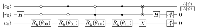
Figure 23: Circuit for full encoding of a 2x2 matrix using big-endian indexing with flipping of encoding block and $\theta_{ij}=2\sin^{-1}(2a_{ij})$.

Appendix C Emulating QSVT

Emulating QSVT on a classical computer can be somewhat frustrating as exactly the same unitaries $U_{A}$ and $U_{A}^{\dagger}$ are applied repeatedly. Computing and storing the unitaries is an effective strategy for small numbers of qubits but the $\mathcal{O}(N^{2})$ scaling of the dense matrix-vector multiplication quickly obviates any advantage. For relatively short encoding circuits, running the circuit in emulation creates the situation where a sequence of sparse matrix-vector multiplications is faster than the corresponding single dense matrix-vector multiplication. In fact, this is always the case, but the cost of circuit emulation soon becomes prohibitive too. Whilst each application of the unitary or its adjoint may not be prohibitive, it is repeating them 100s, 1,000s or even 10,000s of times that becomes prohibitive. The highest degree polynomial used herein had 16,813 phase factors.

The following sub-sections discuss approaches for accelerating QSVT emulators. Of course, QSVT will be run on the quantum computer and the techniques discussed here have no bearing on the speed on a quantum computer. The aim is to enable more rapid progress in algorithm and application development.

All of the following improvements are implemented using big endian ordering. Implementation in little endian ordering is straightforward.

C.1 prepare-select encoding

The first step to accelerate prepare-select encoding is to utilise the fact that the select operator, Equation 13, produces a direct sum of the unitaries:

$$S=\begin{pmatrix}U_{0}&&&\\ &U_{1}&&\\ &&\ddots&\\ &&&U_{M-1}\\ \end{pmatrix}$$ (39)

Applying $S$ to the qubits in QSVT circuit (assuming no other qubits) has the block structure:

$$I\otimes S=\begin{pmatrix}S&0\\ 0&S\\ \end{pmatrix}$$ (40)

Further, each unitary, $U_{i}$, is a tensor product of 1-sparse Pauli matrices. Hence, $S$ is also 1-sparse. If $s_{ij}$ is the only entry on the $i^{th}$ row of $S$ then the application of the unitary maps:

$$\psi_{i} \mapsto s_{ij}\psi_{j}$$ (41)

$$\psi_{i+N} \mapsto s_{ij}\psi_{j+N}$$

where $N$ is the number of rows in $S$. This can be done as an efficient vector multiply using a temporary work vector. Doing this using a sparse matrix data structure carries significant overheads. However, the column indices, which are assumed to be a variable length list, but are actually just a vector, can be extracted to directly perform the vector-vector multiplication.

If the encoding is used within a non-linear solver where the sparsity pattern of the matrix does not change then the Select operator can be constructed once at the outset and reused. This cannot be done if unitaries with small coefficients are trimmed as they is likely to remove different unitaries on each non-linear iteration.

As the prepare operator only acts on the prepare register, it is not initially a bottleneck until the select operator has been streamlined.

Figure 24: prepare circuit for loading 15 LCU coefficients, big endian ordering.

The prepare operator used here is a tree state loader [26]. The levels in the tree correspond to levels in the circuit, as shown in Figure 24. Following Equation 32, the operator for the $2^{nd}$ level in the circuit is:

$$U_{2}=\begin{pmatrix}c_{3}&-s_{3}&0&0&0&0&0&0\\ s_{3}&c_{3}&0&0&0&0&0&0\\ 0&0&c_{4}&-s_{4}&0&0&0&0\\ 0&0&s_{4}&c_{4}&0&0&0&0\\ 0&0&0&0&c_{5}&-s_{5}&0&0\\ 0&0&0&0&s_{5}&c_{5}&0&0\\ 0&0&0&0&0&0&c_{6}&-s_{6}\\ 0&0&0&0&0&0&s_{6}&c_{6}\\ \end{pmatrix}$$ (42)

Applying $U_{2}$ to full prepare-select register requires the a unitary of the form:

$$I\otimes U_{2}\otimes I^{\otimes m}$$ (43)

where $m$ is the number of qubits preceding the tree level in the circuit. This unitary is 2-sparse for all the levels in the tree loader and has the same block structure as Equation 40 when applied to the whole circuit. This can be implemented using by extending the approach used for the select operator:

$$\psi_{i} \mapsto s_{ij}\psi_{j}+s_{ik}\psi_{k}$$ (44)

$$\psi_{i+N} \mapsto s_{ij}\psi_{j+N}+s_{ik}\psi_{k+N}$$

This can be applied to each level of the state loader, but is most beneficial for the lowest levels of the tree which have large numbers of leaves. In practice, levels with small numbers of rotations are executed as a circuit, as this is more efficient than accumulating the equivalent 2-sparse unitary using Equation 43.

Implementing Equation 44 and Equation 41 directly can lead to bespoke code that is harder to maintain. If $U_{2}$ were the full prepare-select dense operator, then expanding Equation 43 to make a full circuit operator can require large amounts of memory and be inefficient to apply. A common alternative is to perform in-situ matrix vector multiplication which strides through the state vector and performs all the multiplications for each matrix entry. However, for 1-sparse and 2-sparse matrices it is more efficient to create the full circuit operator.

C.2 Query Oracle encoding

Efficiently implementing query oracle encoding follows the same approach as separating the prepare and select registers. From Appendix B, the query oracle has a 2x2 block diagonal form:

$$O_{A}=\begin{pmatrix}c_{0}&0&0&0&-s_{0}&0&0&0\\ 0&c_{1}&0&0&0&-s_{1}&0&0\\ 0&0&c_{2}&0&0&0&-s_{2}&0\\ 0&0&0&c_{3}&0&0&0&-s_{3}\\ s_{0}&0&0&0&c_{0}&0&0&0\\ 0&s_{1}&0&0&0&c_{1}&0&0\\ 0&0&s_{2}&0&0&0&c_{2}&0\\ 0&0&0&s_{3}&0&0&0&c_{3}\\ \end{pmatrix}$$ (45)

When applied to the entire QSVT circuit it has the the 4x4 block diagonal structure:

$$I\otimes O_{A}=\begin{pmatrix}C&-S&0&0\\ S&C&0&0\\ 0&0&C&-S\\ 0&0&S&C\\ \end{pmatrix}$$ (46)

This enables an efficient in-situ implementation using 4 local variables:

$$w_{i} =c_{i}\psi_{i}-s_{i}\psi_{i+N/2}$$ (47)

$$w_{i+N/2} =s_{i}\psi_{i}+c_{i}\psi_{i+N/2}$$

$$w_{i+N} =c_{i}\psi_{i+N}-s_{i}\psi_{i+3N/2}$$

$$w_{i+3N/2} =s_{i}\psi_{i+N}+c_{i}\psi_{i+3N/2}$$

$$\psi_{i} =w_{i}$$

$$\psi_{i+N/2} =w_{i+N/2}$$

$$\psi_{i+N} =w_{i+N}$$

$$\psi_{i+3N/2} =w_{i+3N/2}$$

where $N$ is the number of rows in $O_{A}$. An advantage of this formulation is that it is thread safe and it can be easily parallelised using shared or distributed memory programming. The same is not true for the select operator, Equation 41, as the Pauli strings do not, in general, create a block diagonal structure. For arcsin encoding the Pauli X gate s directly implemented in $O_{A}$.

Each of the SWAP operations that follow the query oracle can be efficiently created as a 1-sparse permutation operator acting on the whole circuit. These can be directly implemented as above. Finally, the Hadamard gates are best implemented as individual operations. Assembling tensor products of Hadamard gates creates fully populated operators. Each Hadamard gate is coded as a 2-sparse full circuit operator. Streamlining the SWAP and Hadamard gates may seem like a small benefit, but once the oracle has been optimised, these further reduced the run-time by almost a factor of 4 on 9x9 coupled matrix. Of course, making a fast emulator does not translate to a fast implementation on a quantum device; nor, bring the runtime anywhere near close to the original classical algorithm, but it does enable algorithm research to progress.

References

- [1] D. for Science Innovation and Technology, “National quantum strategy missions.” https://www.gov.uk/government/publications/national-quantum-strategy/national-quantum-strategy-missions, 2023. Accessed: 2024-02-15.
- [2] L. Lapworth, “A hybrid quantum-classical cfd methodology with benchmark hhl solutions,” arXiv preprint arXiv:2206.00419, 2022.
- [3] L. Lapworth, “Implicit hybrid quantum-classical cfd calculations using the hhl algorithm,” arXiv preprint arXiv:2209.07964, 2022.
- [4] A. W. Harrow, A. Hassidim, and S. Lloyd, “Quantum algorithm for linear systems of equations,” Physical review letters, vol. 103, no. 15, p. 150502, 2009.
- [5] A. M. Childs and N. Wiebe, “Hamiltonian simulation using linear combinations of unitary operations,” arXiv preprint arXiv:1202.5822, 2012.
- [6] H. F. Trotter, “On the product of semi-groups of operators,” Proceedings of the American Mathematical Society, vol. 10, no. 4, pp. 545–551, 1959.
- [7] R. Babbush, C. Gidney, D. W. Berry, N. Wiebe, J. McClean, A. Paler, A. Fowler, and H. Neven, “Encoding electronic spectra in quantum circuits with linear t complexity,” Physical Review X, vol. 8, no. 4, p. 041015, 2018.
- [8] D. W. Berry, A. M. Childs, R. Cleve, R. Kothari, and R. D. Somma, “Simulating hamiltonian dynamics with a truncated taylor series,” Physical review letters, vol. 114, no. 9, p. 090502, 2015.
- [9] G. H. Low and I. L. Chuang, “Hamiltonian Simulation by Qubitization,” Quantum, vol. 3, p. 163, July 2019.
- [10] N. Wiebe and S. Zhu, “A theory of trotter error,” Physical Review X, vol. 11, no. 011020, p. 26, 2021.
- [11] J. M. Martyn, Z. M. Rossi, A. K. Tan, and I. L. Chuang, “Grand unification of quantum algorithms,” PRX Quantum, vol. 2, p. 040203, Dec 2021.
- [12] A. Gilyén, Y. Su, G. H. Low, and N. Wiebe, “Quantum singular value transformation and beyond: exponential improvements for quantum matrix arithmetics,” in Proceedings of the 51st Annual ACM SIGACT Symposium on Theory of Computing, pp. 193–204, 2019.
- [13] Y. Dong, X. Meng, K. B. Whaley, and L. Lin, “Efficient phase-factor evaluation in quantum signal processing,” Physical Review A, vol. 103, no. 4, p. 042419, 2021.
- [14] L. Lin, “Lecture notes on quantum algorithms for scientific computation,” arXiv preprint arXiv:2201.08309, 2022.
- [15] B. D. Clader, A. M. Dalzell, N. Stamatopoulos, G. Salton, M. Berta, and W. J. Zeng, “Quantum resources required to block-encode a matrix of classical data,” IEEE Transactions on Quantum Engineering, vol. 3, pp. 1–23, 2022.
- [16] A. M. Childs, R. Kothari, and R. D. Somma, “Quantum algorithm for systems of linear equations with exponentially improved dependence on precision,” SIAM Journal on Computing, vol. 46, no. 6, pp. 1920–1950, 2017.
- [17] S. Chakraborty, A. Gilyén, and S. Jeffery, “The power of block-encoded matrix powers: improved regression techniques via faster hamiltonian simulation,” arXiv preprint arXiv:1804.01973, 2018.
- [18] D. Camps, L. Lin, R. Van Beeumen, and C. Yang, “Explicit quantum circuits for block encodings of certain sparse matrice,” arXiv preprint arXiv:2203.10236, 2022.
- [19] D. Motlagh and N. Wiebe, “Generalized quantum signal processing,” arXiv preprint arXiv:2308.01501, 2023.
- [20] D. Camps and R. Van Beeumen, “Fable: Fast approximate quantum circuits for block-encodings,” in 2022 IEEE International Conference on Quantum Computing and Engineering (QCE), pp. 104–113, IEEE, 2022.
- [21] C. Sünderhauf, E. Campbell, and J. Camps, “Block-encoding structured matrices for data input in quantum computing,” arXiv preprint arXiv:2302.10949, 2023.
- [22] B. Gough, GNU scientific library reference manual. Network Theory Ltd., 2009.
- [23] L. Lapworth, “L-qles: Sparse laplacian generator for evaluating quantum linear equation solvers,” arXiv preprint arXiv:2402.12266, 2024.
- [24] R. Kothari, Efficient algorithms in quantum query complexity. PhD thesis, University of Waterloo, 2014.
- [25] D. W. Berry, M. Kieferová, A. Scherer, Y. R. Sanders, G. H. Low, N. Wiebe, C. Gidney, and R. Babbush, “Improved techniques for preparing eigenstates of fermionic hamiltonians,” npj Quantum Information, vol. 4, no. 1, pp. 1–7, 2018.
- [26] M. Mottonen, J. J. Vartiainen, V. Bergholm, and M. M. Salomaa, “Transformation of quantum states using uniformly controlled rotations,” arXiv preprint quant-ph/0407010, 2004.
- [27] I. F. Araujo, D. K. Park, F. Petruccione, and A. J. da Silva, “A divide-and-conquer algorithm for quantum state preparation,” Scientific Reports, vol. 11, no. 1, pp. 1–12, 2021.
- [28] V. V. Shende, S. S. Bullock, and I. L. Markov, “Synthesis of quantum logic circuits,” arXiv preprint quant-ph/0406176, 2004.
- [29] V. V. Shende, S. S. Bullock, and I. L. Markov, “Synthesis of quantum logic circuits,” in Proceedings of the 2005 Asia and South Pacific Design Automation Conference, pp. 272–275, 2005.
- [30] A. Gilyén, Quantum singular value transformation & its algorithmic applications. PhD thesis, University of Amsterdam, 2019.
- [31] Y. Dong, L. Lin, H. Ni, and J. Wang, “Robust iterative method for symmetric quantum signal processing in all parameter regimes,” arXiv preprint arXiv:2307.12468, 2023.
- [32] G. H. Golub and C. F. Van Loan, Matrix computations. JHU press, 2013.