Constrained Portfolio Analysis in High Dimensions: Tracking Error and Weight Constraints

Abstract

This paper analyzes the statistical properties of constrained portfolio formation in a high dimensional portfolio with a large number of assets. Namely, we consider portfolios with tracking error constraints, portfolios with tracking error jointly with weight (equality or inequality) restrictions, and portfolios with only weight restrictions. Tracking error is the portfolio’s performance measured against a benchmark (an index usually), and weight constraints refers to specific allocation of assets within the portfolio, which often come in the form of regulatory requirement or fund prospectus. We show how these portfolios can be estimated consistently in large dimensions, even when the number of assets is larger than the time span of the portfolio. We also provide rate of convergence results for weights of the constrained portfolio, risk of the constrained portfolio and the Sharpe Ratio of the constrained portfolio. To achieve those results we use a new machine learning technique that merges factor models with nodewise regression in statistics. Simulation results and empirics show very good performance of our method.

Preliminary Draft

1 Introduction

The finance literature related to large portfolio formation and risk and Sharpe Ratio of the large portfolios has not considered compliance-type constraints in the portfolio in statistical analysis. One of the key issues in empirical finance is large portfolio formation. Mainly, the number of assets in a portfolio may be even larger than the time span of the portfolio. However, a related empirical issue is the constraints on large portfolios in practice. One such constraint is tracking error (TE). Tracking error is defined as the standard deviation between fund and the corresponding benchmark’s returns. The mutual fund reports are required to disclose its performance against a benchmark, and usually this is an index, such as SP500 in US, or sector/theme-specific index such as healthcare sector index. Not only is tracking error important for index funds or Exchange Traded Funds (ETF), it serves as a important indicator for risk management and performance evaluation. The tracking error restriction is studied in the past in the finance literature by Rolll (1992), Jorion (2011).

Another key issue in optimal portfolio formation is weight constraints imposed on the portfolio. This type of restriction can be found in fund’s prospectus, and most of the time fund companies would comply with this weight constraint. The weight restriction means that fund manager can invest only on a certain asset class at most a given percentage. For example, the fund can tell at most 20% of non-US stocks can be in the portfolio. These type of constraints are analyzed in U.S. context by Alexander et al. (2004). Also the regulators can impose restrictions in portfolio formation. Bajeux-Besnainou et al. (2011) tells that in France, bond and money market funds cannot hold more than 10% of stocks. In Germany, stocks cannot exceed 35% of the life insurance portfolio, and in Italy it cannot exceed 20% of the portfolio. The weight constraint is sometimes considered jointly with the tracking errors.

We are interested in the following question: can we construct a portfolio that is theoretically guaranteed to be the optimized one given the aforementioned constraints? One of the key issues in the restricted portfolio optimization is the existence of optimal portfolios, which were found and analyzed in Bajeux-Besnainou et al. (2011). However, to this date, there is no high dimensional statistical analysis of these constrained portfolios. By using the factor model literature as developed in Fan et al. (2011), and merged with residual nodewise regression technique as shown in Caner et al. (2023), we analyze constrained portfolios via residual nodewise regression. Specifically, we analyze out-of-sample risk and Sharpe Ratio, and propose estimators for these metrics and also an estimator for the optimal constrained weights in a high dimensional portfolio. This type of research provides us valuable insight into portfolio analysis. We also obtain rates of convergence of our estimators. It is clear that growing number of factors adversely affect the estimation errors as well as the noise. However, we prove in our theorems that our estimators are consistent even when number of assets in the portfolio grows and is larger than the time span of the portfolio. We allow both number of factors, assets and time span to grow although factors grow slower than time span and number of assets.

There are several papers in the past that analyze portfolios, and some of the metrics such as risk and Sharpe Ratio. For example, Fan et al. (2011), Fan et al. (2013) propose principal orthogonal complement thresholding estimator (POET), which analyzes unconstrained large portfolios with a principal components based estimator. Ledoit and Wolf (2017) propose nonlinear shrinkage and single factor shrinkage estimator to estimate covariance matrix of returns and use in financial metrics in an unconstrained portfolio. There is also maximum Sharpe Ratio estimated sparse regression (MAXSER) by Ao et al. (2019), where they can estimate an unconstrained large portfolio when the number of assets grow slower than the time span of the portfolio, and obtain a mean-variance efficient allocation. Those three papers relied on covariance matrix estimation of assets. Callot et al. (2021) provide nodewise regression estimate of the precision matrix of asset returns and obtains consistency results of the estimators of several financial metrics as variance of the portfolio. Recently Caner et al. (2023) merged factor model literature and machine learning to develop residual nodewise regression estimate of the precision matrix of asset returns, and show its consistency in large portfolios. Caner et al. (2023) only analyze the simple restriction of all assets in a portfolio should add up to 100%. Another strand of literature studies weight-constrained portfolios such as Jagannathan and Ma (2003) and DeMiguel et al. (2009). Du et al. (2023) considered high-dimensional portfolio with cardinality constraints. However, none of the aforementioned studies include the compliance-type weight constraint for certain class of assets mentioned above. Compared to all other statistical-econometrics literature we analyze tracking error and inequality constraints on large portfolios. Our simulation and empirical results show strong performance of our proposed method.

Section 2 shows the model. Section 3 considers tracking error constraint. Section 4 has joint analysis of tracking error and equality weights. Section 5 proposes a new estimator for weights of a large portfolio, as well as other metrics, for joint tracking error and inequality constraints. Section 6 has simulations. Section 7 has empirics. Appendix contains all proofs and also case of only weight constraints scenario.

2 Model

We start with the following model, for the $j$ th asset ($j=1,\cdots,p$) excess returns at time $t$ ($t=1,\cdots,T$)

$$y_{j,t}={\boldsymbol{b}_{j}^{\prime}}{\boldsymbol{f}_{t}}+u_{j,t},$$

where ${\boldsymbol{b}_{j}}$ is a $K\times 1$ vector of factor loadings, and ${\boldsymbol{f}_{t}}\mathrel{\mathop{\mathchar 58\relax}}K\times 1$ vector of common factors to all asset returns, and $u_{j,t}$ is the idiosyncratic error term for the $j$ th asset at time $t$. All the factors are observed, and this model is used by Fan et al. (2011). All the vectors and matrices in the paper are in bold. Define the covariance matrix of errors ${\boldsymbol{u}_{t}}=(u_{1,t},\cdots,u_{j,t},\cdots,u_{p,t})^{\prime}\mathrel{\mathop{\mathchar 58\relax}}p\times 1$ vector, as ${\boldsymbol{\Sigma}_{u}}\mathrel{\mathop{\mathchar 58\relax}}=E{\boldsymbol{u}_{t}}{\boldsymbol{u}_{t}}^{\prime}$. We assume $\{({\boldsymbol{f}_{t}},{\boldsymbol{u}_{t}})\}_{t=1}^{T}$ to be a strictly stationary, ergodic, and strong mixing sequence of random vectors. Also, let ${\cal F}_{-\infty}^{0},{\cal F}_{T}^{\infty}$ be the $\boldsymbol{\Sigma}$- algebras generated by $\{({\boldsymbol{f}_{t}},{\boldsymbol{u}_{t}})\}$, for $-\infty<t\leq 0$, and $T\leq t<\infty$, respectively. Denote the strong mixing coefficient as $\alpha(T)\mathrel{\mathop{\mathchar 58\relax}}=\textnormal{sup}_{{\cal A}\in{\cal F}_{-\infty}^{0},{\cal B}\in{\cal F}_{T}^{\infty}}|\mathbb{P}({\cal A})P({\cal B})-\mathbb{P}({\cal A}\cap{\cal B})|.$ Express the asset return matrix as

$${\boldsymbol{y}}={\boldsymbol{B}}{\boldsymbol{X}}+{\boldsymbol{U}},$$

with ${\boldsymbol{y}}\mathrel{\mathop{\mathchar 58\relax}}p\times T$ matrix, and ${\boldsymbol{B}}\mathrel{\mathop{\mathchar 58\relax}}p\times K$ factor loadings matrix, and ${\boldsymbol{X}}=(f_{1},\cdots,f_{T})$ as $K\times T$ matrix of factors, with ${\boldsymbol{U}}$ as $p\times T$ error matrix.

We will assume the sparsity of the precision matrix of errors: ${\boldsymbol{\Omega}}\mathrel{\mathop{\mathchar 58\relax}}={\boldsymbol{\Sigma}_{u}^{-1}}$, and let ${\boldsymbol{\Omega}_{j}^{\prime}}$ be the row vector of ${\boldsymbol{\Omega}}$. In ${\boldsymbol{\Omega}_{j}}^{\prime}$ the indices of non-zero elements of that $j$ th row is denoted as $S_{j}$, for $l=1,\cdots,p$

$$S_{j}\mathrel{\mathop{\mathchar 58\relax}}=\{l\mathrel{\mathop{\mathchar 58\relax}}\Omega_{j,l}\neq 0\},$$

where $\Omega_{j,l}$ be the $j$ th row and $l$ th column element of ${\boldsymbol{\Omega}}$. Let $s_{j}\mathrel{\mathop{\mathchar 58\relax}}=|S_{j}|$ be the cardinality of nonzero elements in row ${\boldsymbol{\Omega}_{j}^{\prime}}$. $s_{j}$ will be nondecreasing in $n$. Denote the maximum number of nonzero elements across each row of ${\boldsymbol{\Omega}}$ as $\bar{s}$, $\bar{s}\mathrel{\mathop{\mathchar 58\relax}}=\max_{1\leq j\leq p}s_{j}$. We use feasible residual based nodewise regression to estimate ${\boldsymbol{\Omega}}$ as shown in Caner et al. (2023). To describe briefly, let ${\bf\hat{b}}_{j}$ denote the $K\times 1$ factor loading estimates by OLS

$${\bf\hat{b}_{j}}=({\boldsymbol{X}}{\boldsymbol{X}}^{\prime})^{-1}{\boldsymbol{X}}{\boldsymbol{y}_{j}},$$

The residual is

$${\bf\hat{u}_{j}}={\bf y_{j}}-{\boldsymbol{X}^{\prime}}{\bf\hat{b}_{j}},$$

with ${\boldsymbol{y}_{j}}=(y_{j,1},\cdots,y_{j,t},\cdots,y_{j,T})^{\prime}\mathrel{\mathop{\mathchar 58\relax}}T\times 1$ vector of excess asset return of $j$ th asset across time. Denote ${\boldsymbol{y}_{-j}}$ as $\bf y$ matrix without the $j$ th row ($p-1\times T$), and it can be expressed as

$${\boldsymbol{y}_{-j}}={\boldsymbol{B}_{-j}}{\boldsymbol{X}}+{\boldsymbol{U}_{-j}},$$

with ${\boldsymbol{B}_{-j}}$ as factor loadings matrix without $j$ th row ($p-1\times K$), and ${\boldsymbol{U}_{-j}}$ as the error matrix without $j$ th row, $j=1,\cdots,p$. Let ${\bf\hat{B}_{-j}}\mathrel{\mathop{\mathchar 58\relax}}(p-1)\times K$ matrix of OLS estimates of factor loadings of ${\boldsymbol{B}_{-j}}$. We have the following residual based matrix which will be used in residual based nodewise regression

$${\bf\hat{U}_{-j}^{\prime}}={\bf y_{-j}^{\prime}}-{\bf X^{\prime}}{\bf\hat{B}_{-j}^{\prime}},$$

with ${\bf\hat{U}_{-j}^{\prime}}\mathrel{\mathop{\mathchar 58\relax}}T\times(p-1)$ matrix, and

$${\bf\hat{B}_{-j}^{\prime}}=({\boldsymbol{X}}{\boldsymbol{X}^{\prime}})^{-1}{\boldsymbol{X}}{\boldsymbol{y}_{-j}^{\prime}},$$

which is $K\times(p-1)$ OLS estimates of factor loadings, except for asset $j$, and $T>K$. The residual based feasible nodewise regression depends on the following, for $j=1,\cdots,p$

$$\hat{\boldsymbol{\gamma}}_{j}=argmin_{\boldsymbol{\gamma}_{j}\in R^{p-1}}\left[\|{\bf\hat{u}_{j}}-{\bf\hat{U}_{-j}^{\prime}}\boldsymbol{\gamma}_{j}\|_{T}^{2}+2\lambda\|{\boldsymbol{\gamma}_{j}}\|_{1}\right],$$ (1)

with $\lambda>0$ as a positive sequence with $\|{\boldsymbol{v}}\|_{T}^{2}$ as the norm with a generic $T\times 1$ vector defined as $\|{\boldsymbol{v}}\|_{T}^{2}\mathrel{\mathop{\mathchar 58\relax}}=\frac{1}{T}\sum_{j=1}^{T}v_{j}^{2}$ . To build the estimate for the precision matrix of errors, we define each row of the precision matrix of errors ${\bf\hat{\Omega}}_{j}^{\prime}\mathrel{\mathop{\mathchar 58\relax}}1\times p$, $j=1,\cdots,p$

$${\bf\hat{\Omega}_{j}^{\prime}}\mathrel{\mathop{\mathchar 58\relax}}={\bf\hat{C}}_{j}^{\prime}/\hat{\tau}_{j}^{2},$$

where ${\bf\hat{C}_{j}^{\prime}}\mathrel{\mathop{\mathchar 58\relax}}1\times p$ row vector with $1$ in the $j$ th cell of that row and the remainder of that row is $-\hat{\boldsymbol{\gamma}}_{j}^{\prime}$. To give an example $\hat{\boldsymbol{C}}_{1}^{\prime}\mathrel{\mathop{\mathchar 58\relax}}=(1,-\hat{\boldsymbol{\gamma}}_{1}^{\prime})\mathrel{\mathop{\mathchar 58\relax}}1\times p$ vector. Also

$$\hat{\tau}_{j}^{2}\mathrel{\mathop{\mathchar 58\relax}}={\bf\hat{u}_{j}^{\prime}}({\bf\hat{u}_{j}}-{\bf\hat{U}_{-j}^{\prime}}\hat{\boldsymbol{\gamma}}_{j})/T,$$

as in Caner et al. (2023). Stacking all rows of ${\bf\hat{\Omega}_{j}^{\prime}}$, we form ${\bf\hat{\Omega}}$, which is residual based feasible nodewise estimate of the precision matrix of errors. Next, we define the covariance matrix of returns

$${\boldsymbol{\Sigma}_{y}}\mathrel{\mathop{\mathchar 58\relax}}={\boldsymbol{B}}({\bf cov\boldsymbol{f}_{t}}){\boldsymbol{B}^{\prime}}+{\boldsymbol{\Sigma}_{u}},$$

with ${\boldsymbol{c}\boldsymbol{o}\boldsymbol{v}\boldsymbol{f}_{t}}$ as the covariance matrix of factors ($K\times K$). By Sherman-Morrison-Woodbury formula, with ${\bf\Theta}\mathrel{\mathop{\mathchar 58\relax}}={\bf\Sigma_{y}^{-1}}$

$$\boldsymbol{\Theta}\mathrel{\mathop{\mathchar 58\relax}}=\boldsymbol{\Omega}-\boldsymbol{\Omega}\boldsymbol{B}[(\boldsymbol{c}\boldsymbol{o}\boldsymbol{v}\boldsymbol{f}_{t})^{-1}+\boldsymbol{B}^{\prime}\boldsymbol{\Omega}\boldsymbol{B}]^{-1}\boldsymbol{B}^{\prime}\boldsymbol{\Omega},$$

and its estimate based on residual based feasible nodewise estimate of errors is:

$$\hat{\boldsymbol{\Theta}}\mathrel{\mathop{\mathchar 58\relax}}=\hat{\boldsymbol{\Omega}}-\hat{\boldsymbol{\Omega}}\hat{\boldsymbol{B}}[(\widehat{\boldsymbol{c}\boldsymbol{o}\boldsymbol{v}\boldsymbol{f}_{t}})^{-1}+\hat{\boldsymbol{B}}^{\prime}\hat{\boldsymbol{\Omega}}_{sym}\hat{\boldsymbol{B}}]^{-1}\hat{\boldsymbol{B}}^{\prime}\hat{\boldsymbol{\Omega}},$$

with $\widehat{\boldsymbol{c}\boldsymbol{o}\boldsymbol{v}\boldsymbol{f}_{t}}\mathrel{\mathop{\mathchar 58\relax}}T^{-1}\boldsymbol{X}\boldsymbol{X}^{\prime}-T^{-2}\boldsymbol{X}\boldsymbol{1}_{T}\boldsymbol{1}_{T}^{\prime}\boldsymbol{X}^{\prime}$, with $\boldsymbol{1}_{T}$ representing a $T\times 1$ vector of ones, and $\hat{\boldsymbol{\Omega}}_{sym}\mathrel{\mathop{\mathchar 58\relax}}=\frac{1}{2}[\hat{\boldsymbol{\Omega}}+\hat{\boldsymbol{\Omega}}^{\prime}]$, $\hat{\boldsymbol{B}}^{\prime}=(\boldsymbol{X}\boldsymbol{X}^{\prime})^{-1}\boldsymbol{X}\boldsymbol{y}\mathrel{\mathop{\mathchar 58\relax}}K\times p$ matrix.

Before assumptions we make clear an important point, we allow both $p$ (no of assets), $K$ (no of factors) grow when $T$ increases. To save notation we do not subscript $p,K$ with $T$. We also restrict $min(p,T)>K$.

2.1 Assumptions

In this subsection, we provide the assumptions. But before that we need the following notation. We use the following notation in the paper regarding vector and matrix norms. Let $\boldsymbol{v}$ be a generic $n\times 1$ vector and $\boldsymbol{H}$ to be a generic $n\times n$ matrix. Then $\|\boldsymbol{v}\|_{1},\|\boldsymbol{v}\|_{2},\|\boldsymbol{v}\|_{\infty}$ are the $l_{1}$, Euclidean, and sup norms of the vector $\boldsymbol{v}$ respectively. Next, $\|\boldsymbol{H}\|_{l_{1}},\|\boldsymbol{H}\|_{l_{\infty}}$ are the maximum column sum matrix norm, and maximum row sum matrix norm respectively. This means $\|\boldsymbol{H}\|_{l_{1}}\mathrel{\mathop{\mathchar 58\relax}}=\max_{1\leq j\leq n}\sum_{i=1}^{n}|H_{i,j}|$, and $\|\boldsymbol{H}\|_{l_{\infty}}\mathrel{\mathop{\mathchar 58\relax}}=\max_{1\leq i\leq n}\sum_{j=1}^{n}|H_{i,j}|$, where $H_{i,j}$ represents $(i,j)$ th element of matrix $H$. Let $\|\boldsymbol{H}\|_{l_{2}}$ be the spectral norm of matrix H, and $\|\boldsymbol{H}\|_{\infty}\mathrel{\mathop{\mathchar 58\relax}}=\max_{1\leq i\leq n}\max_{1\leq j\leq n}|H_{i,j}|$.

First, $\boldsymbol{u}_{-j,t}$ is the $(p-1)\times 1$ vector of errors in $t$ th time period, except the $j$th term in $\boldsymbol{u}_{t}$. Then define $\eta_{j,t}\mathrel{\mathop{\mathchar 58\relax}}=u_{j,t}-\boldsymbol{u}_{-j,t}^{\prime}\boldsymbol{\gamma}_{j}$. Also define $Eigmin(\boldsymbol{A})$ to be the minimum eigenvalue of the matrix ${\boldsymbol{A}}$.

Assumption 1.

(i). $\{\boldsymbol{u}_{t}\}_{t=1}^{T},\{\boldsymbol{f}_{t}\}_{t=1}^{T}$ are sequences of (strictly) stationary and ergodic random vectors . Furthermore, $\{\boldsymbol{u}_{t}\}_{t=1}^{T},\{\boldsymbol{f}_{t}\}_{t=1}^{T}$ are independent. $\boldsymbol{u}_{t}$ is a ($p\times 1$) zero mean random vector with covariance matrix $\boldsymbol{\Sigma}_{u}$ ($p\times p$). $\textnormal{Eigmin}(\boldsymbol{\Sigma}_{u})\geq c>0$, with $c$ a positive constant, and $\max_{1\leq j\leq p}\mathbb{E}\left[u_{j,t}^{2}\right]\leq C<\infty$. (ii). For the strong mixing vector of random variables $\boldsymbol{f}_{t},\boldsymbol{u}_{t}$: $\alpha(t)\leq\exp(-Ct^{r_{0}})$, for a positive constant $r_{0}>0$.

Assumption 2.

There exists positive constants $r_{1}$, $r_{2}$, $r_{3}>0$ and another set of positive constants $c_{1}$, $c_{2}$, $c_{3}$, $s_{1}$, $s_{2}$, $s_{3}>0$, and for $t=1,\cdots,T$, and $j=1,\cdots,p$, with $k=1,\cdots,K$

(i).

$$\mathbb{P}\left[|u_{j,t}|>s_{1}\right]\leq\exp[-(s_{1}/c_{1})^{r_{1}}].$$

(ii).

$$\mathbb{P}\left[|\eta_{j,t}|>s_{2}\right]\leq\exp[-(s_{2}/c_{2})^{r_{2}}].$$

(iii).

$$\mathbb{P}\left[|f_{k,t}|>s_{3}\right]\leq\exp[-(s_{3}/c_{3})^{r_{3}}].$$

(iv). There exists $0<\phi_{1}<1$ such that $\phi_{1}^{-1}=3r_{1}^{-1}+r_{0}^{-1}$, and we also assume $3r_{2}^{-1}+r_{0}^{-1}>1$, and $3r_{3}^{-1}+r_{0}^{-1}>1$.

Define $\phi_{2}^{-1}\mathrel{\mathop{\mathchar 58\relax}}=1.5r_{1}^{-1}+1.5r_{2}^{-1}+r_{0}^{-1}$, and $\phi_{3}^{-1}\mathrel{\mathop{\mathchar 58\relax}}=1.5r_{1}^{-1}+1.5r_{3}^{-1}+r_{0}^{-1}$, let $\phi_{\min}\mathrel{\mathop{\mathchar 58\relax}}=\min(\phi_{1},\phi_{2},\phi_{3})$.

Assumption 3.

(i). $[\ln(p)]^{(2/\phi_{min})-1}=o(T)$, and (ii). $K^{2}=o(T)$, (iii). $K=o(p)$.

Assumption 4.

(i). $Eigmin[\boldsymbol{c}ov(\boldsymbol{f}_{t})]\geq c>0$, with $\boldsymbol{c}ov(\boldsymbol{f}_{t})$ being the covariance matrix of the factors $\boldsymbol{f}_{t}$, $t=1,\cdots,T$. (ii). $\max_{1\leq k\leq K}\mathbb{E}\left[f_{kt}^{2}\right]\leq C<\infty$, $\min_{1\leq k\leq k}\mathbb{E}\left[f_{kt}^{2}\right]\geq c>0$. (iii). $\max_{1\leq j\leq p}\mathbb{E}\left[\eta_{j,t}^{2}\right]\leq C<\infty$.

Assumption 5.

(i).

$$\max_{1\leq j\leq p}\max_{1\leq k\leq K}|b_{jk}|\leq C<\infty.$$

(ii).

$$\|p^{-1}\boldsymbol{B}^{\prime}\boldsymbol{B}-\boldsymbol{\Phi}\|_{l_{2}}=o(1),$$

for some $K\times K$ symmetric positive definite matrix $\boldsymbol{\Phi}$ such that $Eigmin(\boldsymbol{\Phi})$ is bounded away from zero.

Assumption 6.

$Eigmax(\boldsymbol{\Sigma}_{u})\leq Cr_{T}$ with $C>0$ a positive constant, and $r_{T}\to\infty$ as $T\to\infty$ and $r_{T}/p\to 0$ and $r_{T}$ is a positive sequence.

Define the rate

$$l_{T}\mathrel{\mathop{\mathchar 58\relax}}=r_{T}^{2}K^{5/2}\max(\bar{s}\lambda,\bar{s}^{1/2}K^{1/2}\sqrt{\frac{\max[lnp,lnT]}{T}}).$$ (2)

Given that $\boldsymbol{\mu}\mathrel{\mathop{\mathchar 58\relax}}=(\mu_{1},\cdots,\mu_{j},\cdots,\mu_{p})^{\prime}$ is the expected portfolio return vector and $\boldsymbol{m}$ being the benchmark portfolio, and $\boldsymbol{w}_{d}^{*}\mathrel{\mathop{\mathchar 58\relax}}=\boldsymbol{w}-\boldsymbol{m}$, with $\boldsymbol{w}$ being the portfolio of interest

Assumption 7.

(i). $\bar{s}^{3}l_{T}r_{T}^{2}K^{8}=o(1)$.

(ii). $\frac{\boldsymbol{\mu}^{\prime}\boldsymbol{\Theta}\boldsymbol{\mu}}{p}\geq c>0,\frac{\boldsymbol{1}_{p}^{\prime}\boldsymbol{\Theta}\boldsymbol{1}_{p}}{p}\geq c>0$, with $c$ being a positive constant.

(iii). $\|\boldsymbol{m}\|_{1}=O(\|\boldsymbol{w}_{d}^{*}\|_{1})$, $\boldsymbol{w}^{*^{\prime}}\boldsymbol{\Sigma}_{y}\boldsymbol{w}^{*}\geq c>0$, $|\boldsymbol{w}^{*^{\prime}}\boldsymbol{\mu}|\geq c>0$.

Assumptions 1-4 are used in Caner et al. (2023) to provide the consistency of the precision matrix estimator for errors. Note that Assumptions 1-3 are standard assumptions and are also used in Fan et al. (2011) as well. Also, we get $0<\phi_{2}<1,0<\phi_{3}<1$ given Assumption 2(iv). Furthermore, by Assumption 3, $\sqrt{\frac{\ln(p)}{T}}=o(1)$. Note that, Stationary GARCH models with finite second moments and continuous error distributions, as well as causal ARMA processes with continuous error distributions, and a certain class of stationary Markov chains satisfy our Assumptions 1-2 and are discussed in p.61 of Chang et al. (2018).

Assumption 4(i)-(ii) is also used in Fan et al. (2011), and the nodewise error assumption 4(iii) is used in Caner and Kock (2018). Next, we provide assumptions that are used to obtain consistency of the estimate of the precision matrix of returns in Caner et al. (2023). Assumption 5 is used in Fan et al. (2011). It puts some structure on the factor loadings, and this is also used in Caner et al. (2023). Assumption 6 allows the maximal eigenvalue of $\boldsymbol{\Sigma}_{u}$ to grow with T, and is used also Gagliardini et al. (2016), and also used in Caner et al. (2023). Assumption 7(i) is a tradeoff between sparsity, number of factors and eigenvalue conditions. This is more restrictive than sparsity Assumption 8 in Caner et al. (2023). Assumption 7(ii) shows that square of the maximum Sharpe Ratio (unconstrained) is lower bounded by a positive constant. This is scaled by $p$ since the numerator is summed over $p$. Then the second part of Assumption 7(ii) imposes that Global Minimum Variance (unconstrained) portfolio variance is finite. Assumption 7(ii) is used in Caner et al. (2023). Note that (16) of Caner et al. (2023) finds $\lambda=O(\sqrt{lnp/T})$ under Assumptions 1-4. Assumption 7(iii) assigns the benchmark portfolio to be growing at most as the optimal tracking error portfolio in $l_{1}$ norm in Section 3 below, and this is just needed to show that benchmark and optimal portfolios have similar behavior in $l_{1}$ norm. The rest of Assumption 7 constrains the optimal variance to be positive, and absolute portfolio return to be bounded away from zero. To show that Assumption 7 is plausible, we can have the following example, without losing any generality, with $p=2T,\bar{s}=lnT,K=lnT,r_{T}=T^{1/9}$, then

$$l_{T}=T^{2/9}(ln(T))^{5/2}\max[ln(T)\sqrt{ln(2T)/T},(ln(T))^{1/2}(ln(T))^{1/2}\sqrt{ln(2T)/T}]=T^{2/9}(ln(T))^{7/2}\sqrt{ln2T/T}.$$

Then

$$\bar{s}^{3}l_{T}r_{T}^{2}K^{8}=T^{4/9}(ln(T))^{11+7/2}\sqrt{ln(2T)/T}\to 0.$$

We also show the portfolios that are defined in Sections 2-4, and the rates that are used. Since the notation is heavy in this paper, that may help the reader. All the definitions of mentioned portfolios and rates of convergence are given in Sections below. Section 2 the portfolios are $\boldsymbol{w},\boldsymbol{w}^{*},\boldsymbol{m},\boldsymbol{w}_{d},\boldsymbol{w}_{d}^{*}$, and the rates are $r_{T}\to\infty,T\to\infty,l_{T}\to 0,T\to\infty$, as well as $r_{w1}\to 0,T\to\infty$. We do not have subscripts for $\bar{s},K$ since they can be constants or growing with $T$. Section 3 portfolios are $\boldsymbol{l},\boldsymbol{k},\boldsymbol{a},\boldsymbol{w}_{cp}^{*},\boldsymbol{w}_{R}^{*},\boldsymbol{w}_{c}^{*}$. The rate in Section 3 is $r_{w2}\to 0,T\to\infty$. For Section 4, portfolios are $\boldsymbol{w}_{op}^{*},\boldsymbol{w}_{est}^{*}$.

We differentiated our rates of convergence of weights under different constraints as $r_{w1},r_{w2}$ and did not put an additional subscript $T$, all the other rates have $T$ subscript.

3 Tracking Error Constraint

We want to maximize the expected return with a tracking error constraint as in Bajeux-Besnainou et al. (2011).

$$\max_{\boldsymbol{w}\in R^{p}}\boldsymbol{\mu}^{\prime}\boldsymbol{w}\quad\mbox{subject to}\quad(\boldsymbol{w}-\boldsymbol{m})^{\prime}\boldsymbol{\Sigma}_{y}(\boldsymbol{w}-\boldsymbol{m})\leq TE^{2},\quad\boldsymbol{1}_{p}^{\prime}\boldsymbol{w}=1,$$

with $\boldsymbol{m}\mathrel{\mathop{\mathchar 58\relax}}p\times 1$ benchmark portfolio of weights, $\boldsymbol{w}$ is the portfolio of weights that is tracking the benchmark portfolio $\boldsymbol{m}$, $\boldsymbol{\mu}\mathrel{\mathop{\mathchar 58\relax}}p\times 1$ vector of expected return on assets, and $TE$ is the tracking error. Alternatively we can write the optimization as

$$\boldsymbol{w}_{d}^{*}\mathrel{\mathop{\mathchar 58\relax}}=\max_{\boldsymbol{w}_{d}\in R^{p}}[\boldsymbol{\mu}^{\prime}\boldsymbol{w}_{d}-\frac{\Xi}{2}\boldsymbol{w}_{d}^{\prime}\boldsymbol{\Sigma}_{y}\boldsymbol{w}_{d}],\quad\mbox{subject to}\quad\boldsymbol{1}_{p}^{\prime}\boldsymbol{w}_{d}=0,$$

with $\boldsymbol{w}_{d}=\boldsymbol{w}-\boldsymbol{m}$, $\infty>\Xi>0$, where $\Xi$ can be roughly seen as a risk aversion parameter. The solution to above problem is, $\boldsymbol{\Theta}\mathrel{\mathop{\mathchar 58\relax}}=\boldsymbol{\Sigma}_{y}^{-1}$, as in (1) of Bajeux-Besnainou et al. (2011)

$$\boldsymbol{w}_{d}^{*}=\kappa\left[\frac{\boldsymbol{\Theta}\boldsymbol{\mu}}{\boldsymbol{1}_{p}^{\prime}\boldsymbol{\Theta}\boldsymbol{\mu}}-\frac{\boldsymbol{\Theta}\boldsymbol{1}_{p}}{\boldsymbol{1}_{p}^{\prime}\boldsymbol{\Theta}\boldsymbol{1}_{p}}\right],$$ (3)

where $\frac{\boldsymbol{\Theta}\boldsymbol{\mu}}{\boldsymbol{1}_{p}^{\prime}\boldsymbol{\Theta}\boldsymbol{\mu}}$ is the portfolio that maximizes Sharpe ratio, and $\frac{\boldsymbol{\Theta}\boldsymbol{1}_{p}}{\boldsymbol{1}_{p}^{\prime}\boldsymbol{\Theta}\boldsymbol{1}_{p}}$ is the standard global minimum variance portfolio. Let $c,C$ be positive constants. Then $\kappa$, represents the risk tolerance parameter, which is described in equation (5) of Bajeux-Besnainou et al. (2011), with range of $0<c\leq|\kappa|\leq C<\infty$. For risk averse investors $0<c\leq\kappa\leq C<\infty$. $\kappa,\boldsymbol{m}$ are given by investors and not estimated. The relation between $TE,\kappa,\Xi$ is given in Section A.2. The aim is to estimate optimal weights $\boldsymbol{w}_{d}^{*}$, and $\boldsymbol{w}^{*}\mathrel{\mathop{\mathchar 58\relax}}=\boldsymbol{w}_{d}^{*}+\boldsymbol{m}$. In that respect we provide the following estimate

$$\hat{\boldsymbol{w}}_{d}=\kappa\left[\frac{\hat{\boldsymbol{\Theta}}^{\prime}\hat{\boldsymbol{\mu}}}{\boldsymbol{1}_{p}^{\prime}\hat{\boldsymbol{\Theta}}^{\prime}\hat{\boldsymbol{\mu}}}-\frac{\hat{\boldsymbol{\Theta}}^{\prime}\boldsymbol{1}_{p}}{\boldsymbol{1}_{p}^{\prime}\hat{\boldsymbol{\Theta}}\boldsymbol{1}_{p}}\right],$$

with $\hat{\boldsymbol{\mu}}=\frac{1}{T}\sum_{t=1}^{T}\boldsymbol{y}_{t}$, with $y_{t},t=1,\cdots,T$ being the columns of $\boldsymbol{y}$ matrix. Note that since

$$\hat{\boldsymbol{w}}=\hat{\boldsymbol{w}}_{d}+\boldsymbol{m},$$ (4)

we have

$$\|\hat{\boldsymbol{w}}_{d}-\boldsymbol{w}_{d}^{*}\|_{1}=\|\hat{\boldsymbol{w}}-\boldsymbol{w}^{*}\|_{1},$$

given $\hat{\boldsymbol{w}}=\hat{\boldsymbol{w}}_{d}+\boldsymbol{m}$. We provide the following theorem, that shows that portfolio weights can be consistently estimated in a large portfolio with tracking error constraint.

Also we have two other metrics that we consider. Out-of-sample variance of a portfolio, and out-of-sample-Sharpe-Ratio corresponding to constrained portfolio weight estimates $\hat{\boldsymbol{w}}$. Specifically they are, the out of sample variance estimate of the constrained portfolio

$$\hat{\boldsymbol{w}}^{\prime}\boldsymbol{\Sigma}_{y}\hat{\boldsymbol{w}},$$ (5)

and the estimate of the out-of-sample-Sharpe-Ratio of the constrained portfolio

$$\widehat{SR}=\frac{\hat{\boldsymbol{w}}^{\prime}\boldsymbol{\mu}}{\sqrt{\hat{\boldsymbol{w}}^{\prime}\boldsymbol{\Sigma}_{y}\hat{\boldsymbol{w}}}}.$$ (6)

The Sharpe ratio is $SR=\boldsymbol{w}^{*^{\prime}}\boldsymbol{\mu}/\sqrt{\boldsymbol{w}^{*^{\prime}}\boldsymbol{\Sigma}_{y}\boldsymbol{w}^{*}}$.

Define the rate $r_{w1}\mathrel{\mathop{\mathchar 58\relax}}=\bar{s}^{2}l_{T}r_{T}K^{7/2}$. Note that $l_{T}\to 0$ and is defined in (2), and $r_{T}\to\infty$ with $T\to\infty$, and is defined in Assumption 6, and $\bar{s}$ is nondecreasing in $T$, and also $K$ is nondecreasing in $T$. We provide consistent estimation of portfolio weights and out-of-sample variance of the constrained portfolio.

Theorem 1.

Under Assumptions 1-7, with the following condition $|\boldsymbol{1}_{p}^{\prime}\boldsymbol{\Theta}\boldsymbol{\mu}|/p\geq c>0$, with $c$ being a positive constant, and $0<c\leq|\kappa|\leq C<\infty$

(i).

$$\|\hat{\boldsymbol{w}}-\boldsymbol{w}^{*}\|_{1}=\|\hat{\boldsymbol{w}}_{d}-\boldsymbol{w}_{d}^{*}\|_{1}=O_{p}(r_{w1})=O_{p}(\bar{s}^{2}l_{T}r_{T}K^{7/2})=o_{p}(1).$$

(ii).

$$\left|\frac{\hat{\boldsymbol{w}}^{{}^{\prime}}\boldsymbol{\Sigma}_{y}\hat{\boldsymbol{w}}}{\boldsymbol{w}^{*^{\prime}}\boldsymbol{\Sigma}_{y}\boldsymbol{w}^{*}}-1\right|=O_{p}(r_{w1}\bar{s}r_{T}K^{9/2})=O_{p}(\bar{s}^{3}l_{T}r_{T}^{2}K^{8})=o_{p}(1).$$

(iii).

$$\left|\left[\frac{\widehat{SR}}{SR}\right]^{2}-1\right|=O_{p}(r_{w1}\bar{s}r_{T}K^{9/2})=O_{p}(\bar{s}^{3}l_{T}r_{T}^{2}K^{8})=o_{p}(1).$$

Remarks. 1. These are all new results in the literature and allows $p>T$, and both can grow to $\infty$ due to $l_{T}$ definition in (2). An example of a rate is given at the end of section 1. Corollary 3 of Caner et al. (2023) shows unconstrained maximum out of sample Sharpe ratio can be consistenly estimated with a rate of $\bar{s}l_{T}K^{2}$, so our Theorem 1(iii) here shows the effect of the tracking error constraint, and our estimation error is much larger.

2. $|\boldsymbol{1}_{p}^{\prime}\boldsymbol{\Theta}\boldsymbol{\mu}/p|=p^{-1}|\sum_{j=1}^{p}\sum_{k=1}^{p}\Theta_{j,k}\mu_{k}|\geq c>0$ is a very mild condition that prevents expected scaled-mean to be a very small number near zero. See also Remark 3 of Theorem 7 in Caner et al. (2023) for this point.

3. If the precision matrix of errors is non-sparse we can have $\bar{s}=p$. Then in this case $p<T$, and we need $p^{2}l_{T}r_{T}K^{7/2}=o(1)$, hence we need $p=o(T^{1/4})$, by using $l_{T}$ definition in (2) for Theorem 1(i). For Theorems 1(ii)-(iii), with non-sparse $\bar{s}=p$, we need $p=o(T^{1/6})$.

4. We can also have an estimate for tracking error as $\widehat{TE}_{d}\mathrel{\mathop{\mathchar 58\relax}}=\sqrt{\hat{\boldsymbol{w}}_{d}^{\prime}\boldsymbol{\Sigma}_{y}\hat{\boldsymbol{w}}_{d}}$, as an out-sample estimate. It can easily be shown that $|(\frac{\widehat{TE}_{d}}{TE})^{2}-1|$ will converge in probability to zero by following the proof of Theorem 1(ii), and the rate will be the same as in Theorem 1(ii). This estimator is consistent.

5. Note that estimating variance and Sharpe Ratio is more difficult compared to weight formation. This is clear by comparing Theorem 1(i) with Theorem 1(ii)(iii). We can also estimate in-sample Sharpe Ratio with our analysis as in Caner et al. (2023) but out-sample one is more related to portfolio advice in practice, hence we analyze out-sample here.

4 Joint Tracking Error and Weight Constraints

In this section we analyze weight constraints for a portfolio. Let $R$ represent the indices of restrictions and we define the cardinality of the set $R$ as $r\mathrel{\mathop{\mathchar 58\relax}}=|R|$. We allow for at least 1 restricted asset and also all the assets cannot be restricted. In other words, if the number of restrictions are $r$, $1\leq r<p$. To give an example, let $p=10$, and $R=\{1,5,7\}$, this means assets 1, 5, 7 are restricted in an 10 asset portfolio, and $r=3$. To make things a bit clear in notation, define $\boldsymbol{1}_{R}$ as a $p\times 1$ vector where we have ones in the places of restricted assets, and zeroes in the unrestricted assets. To continue with the example above $1_{R}=(1,0,0,0,1,0,1,0,0,0)^{\prime}$. Define $\bar{w}\mathrel{\mathop{\mathchar 58\relax}}=\boldsymbol{1}_{R}^{\prime}\boldsymbol{w}-\boldsymbol{1}_{R}^{\prime}\boldsymbol{m}=\boldsymbol{1}_{R}^{\prime}\boldsymbol{w}_{d}$. Then $\boldsymbol{w}_{cp}$ is the difference between the portfolio and the benchmark portfolio when both benchmark and the portfolio is restricted. The constraints may take the form of certain stocks wanted to be excluded from the portfolio from the perspective of financial, moral, ethical and religious considerations. We allow for $r\to\infty$ as $p\to\infty$ as long as $0<\frac{r}{p}<1$. We allow for equality constraints of the form

$$\bar{w}=\omega,$$

where $\omega$ can be positive or negative. This representation is adopted by Bajeux-Besnainou et al. (2011). To give an example $\omega=0$ may show same restrictions applied to benchmark, $\boldsymbol{m}$, should apply to portfolio that we are forming, $\boldsymbol{w}$. To continue with that simple example with 10 assets above, if $\boldsymbol{1}_{R}^{\prime}\boldsymbol{w}=0.6$ means the weight of combined assets 1, 5 and 7 should be 0.6. If the weights are normalized to one and there is no short selling allowed, this means we form 60% of our portfolio from these three assets. These are very common restrictions in portfolio formation either by funds themselves or governments. This 60% can represent the percentage of stocks in a portfolio, for example. The optimization problem is:

$$\boldsymbol{w}_{cp}^{*}\mathrel{\mathop{\mathchar 58\relax}}=\max_{\boldsymbol{w}_{d}\in R^{P}}[\boldsymbol{\mu}^{\prime}\boldsymbol{w}_{d}-\frac{\boldsymbol{\Xi}}{2}\boldsymbol{w}_{d}^{\prime}\boldsymbol{\Sigma}_{y}\boldsymbol{w}_{d}],\quad\mbox{subject to}\quad\boldsymbol{1}_{p}^{\prime}\boldsymbol{w}_{d}=0,\quad\boldsymbol{1}_{R}^{\prime}\boldsymbol{w}_{d}=\omega.$$

The solution is given by Proposition 1 in Bajeux-Besnainou et al. (2011). This is basically the solution to tracking error portfolio added to a fraction of the portfolio $\boldsymbol{l}$ where $\boldsymbol{l}$ can be thought as the weighted difference between restricted and unrestricted minimum variance portfolios.

$$\boldsymbol{w}_{cp}^{*}=(\omega-\kappa w_{u})\boldsymbol{l}+\boldsymbol{w}_{d}^{*}=(\omega-\kappa w_{u})\boldsymbol{l}+(\boldsymbol{w}^{*}-\boldsymbol{m}),$$ (7)

with

$$\boldsymbol{l}\mathrel{\mathop{\mathchar 58\relax}}=\frac{\boldsymbol{k}-\boldsymbol{a}}{w_{k}-w_{a}},$$

and

$$\boldsymbol{k}\mathrel{\mathop{\mathchar 58\relax}}=\frac{\boldsymbol{\Theta}\boldsymbol{1}_{R}}{\boldsymbol{1}_{p}^{\prime}\boldsymbol{\Theta}\boldsymbol{1}_{R}},\quad\boldsymbol{a}\mathrel{\mathop{\mathchar 58\relax}}=\frac{\boldsymbol{\Theta}\boldsymbol{1}_{p}}{\boldsymbol{1}_{p}^{\prime}\boldsymbol{\Theta}\boldsymbol{1}_{p}},$$

which are fully invested portfolios, and $\boldsymbol{a}$ is the minimum variance portfolio, and $\boldsymbol{k}$ can be thought roughly as its restricted counterpart. Note that $w_{k}$ is the addition of weights in the restricted minimum variance portfolio, and $w_{a}$ below represents the addition of weights in the minimum variance portfolio. Set

$$w_{k}-w_{a}=\frac{\boldsymbol{1}_{R}^{\prime}\boldsymbol{\Theta}\boldsymbol{1}_{R}}{\boldsymbol{1}_{R}^{\prime}\boldsymbol{\Theta}\boldsymbol{1}_{p}}-\frac{\boldsymbol{1}_{R}^{\prime}\boldsymbol{\Theta}\boldsymbol{1}_{p}}{\boldsymbol{1}_{p}^{\prime}\boldsymbol{\Theta}\boldsymbol{1}_{p}},$$

and $w_{k}\neq w_{a}$ since by assumption all assets in the portfolio cannot be restricted. We also have scalar

$$w_{u}=\boldsymbol{1}_{R}^{\prime}[\frac{\boldsymbol{\Theta}\boldsymbol{\mu}}{\boldsymbol{1}_{p}^{\prime}\boldsymbol{\Theta}\boldsymbol{\mu}}-\frac{\boldsymbol{\Theta}\boldsymbol{1}_{p}}{\boldsymbol{1}_{p}^{\prime}\boldsymbol{\Theta}\boldsymbol{1}_{p}}],$$ (8)

where $w_{u}$ can be thought as the subtraction of minimum variance portfolio weights from maximum Sharpe Ratio portfolio weights, when only restricted assets are taken into account. We can also rewrite the optimal joint restricted portfolio as

$$\boldsymbol{w}_{cp^{*}}=\omega\boldsymbol{l}+\boldsymbol{w}_{d}^{*}-\kappa w_{u}\boldsymbol{l},$$

where $\omega\boldsymbol{l}$ is the constrained minimum TE portfolio, and the additional weights $(w_{d}^{*}-\kappa w_{u}\boldsymbol{l})$ has zero weight on restricted assets, and provide additional return by increasing TE, as discussed by p.306 of Bajeux-Besnainou et al. (2011).

The estimator can be obtained by using the estimate $\hat{\boldsymbol{\Theta}}$ , with

$$\widehat{\boldsymbol{w}}_{cp}=(\omega-\kappa\hat{w}_{u})\hat{\boldsymbol{l}}+\hat{\boldsymbol{w}}_{d},$$ (9)

with

$$\hat{\boldsymbol{l}}=\frac{\hat{\boldsymbol{k}}-\hat{\boldsymbol{a}}}{\hat{w}_{k}-\hat{w}_{a}},$$

and

$$\hat{\boldsymbol{k}}=\frac{\hat{\boldsymbol{\Theta}}^{\prime}\boldsymbol{1}_{R}}{\boldsymbol{1}_{p}^{\prime}\hat{\boldsymbol{\Theta}}^{\prime}\boldsymbol{1}_{R}},\quad\hat{\boldsymbol{a}}=\frac{\hat{\boldsymbol{\Theta}}^{\prime}\boldsymbol{1}_{p}}{\boldsymbol{1}_{p}^{\prime}\hat{\boldsymbol{\Theta}}^{\prime}\boldsymbol{1}_{p}},$$

with

$$\hat{w}_{k}-\hat{w}_{a}=\frac{\boldsymbol{1}_{R}^{\prime}\hat{\boldsymbol{\Theta}}^{\prime}\boldsymbol{1}_{R}}{\boldsymbol{1}_{R}^{\prime}\hat{\boldsymbol{\Theta}}^{\prime}\boldsymbol{1}_{p}}-\frac{\boldsymbol{1}_{R}^{\prime}\hat{\boldsymbol{\Theta}}^{\prime}\boldsymbol{1}_{p}}{\boldsymbol{1}_{p}^{\prime}\hat{\boldsymbol{\Theta}}^{\prime}\boldsymbol{1}_{p}},$$

and $\hat{w_{k}}\neq\hat{w}_{a}$ since by assumption all assets in the portfolio cannot be restricted. We also have

$$\hat{w}_{u}=\frac{\boldsymbol{1}_{R}^{\prime}\hat{\boldsymbol{\Theta}}^{\prime}\boldsymbol{\mu}}{\boldsymbol{1}_{p}^{\prime}\hat{\boldsymbol{\Theta}}^{\prime}\boldsymbol{\mu}}-\frac{\boldsymbol{1}_{R}^{\prime}\hat{\boldsymbol{\Theta}}^{\prime}\boldsymbol{1}_{p}}{\boldsymbol{1}_{p}^{\prime}\hat{\boldsymbol{\Theta}}^{\prime}\boldsymbol{1}_{p}}.$$

First define the restricted benchmark portfolio as $\boldsymbol{m}_{R}$ as the benchmark portfolio. Define $\boldsymbol{w}_{R}^{*}\mathrel{\mathop{\mathchar 58\relax}}=\boldsymbol{w}_{cp}^{*}+\boldsymbol{m}_{R}$ and

$$\hat{\boldsymbol{w}}_{R}\mathrel{\mathop{\mathchar 58\relax}}=\hat{\boldsymbol{w}}_{cp}+\boldsymbol{m}_{R}.$$ (10)

Define now the Sharpe Ratio associated with joint restrictions of TE and weight:

$$SR_{R}\mathrel{\mathop{\mathchar 58\relax}}=\frac{\boldsymbol{w}_{R}^{*^{\prime}}\boldsymbol{\mu}}{\sqrt{\boldsymbol{w}_{R}^{*^{\prime}}\boldsymbol{\Sigma}_{y}\boldsymbol{w}_{R}^{*}}},$$

and estimate

$$\widehat{SR}_{R}\mathrel{\mathop{\mathchar 58\relax}}=\frac{\hat{\boldsymbol{w}}_{R}^{\prime}\boldsymbol{\mu}}{\sqrt{\hat{\boldsymbol{w}}_{R}}^{\prime}\boldsymbol{\Sigma}_{y}\hat{\boldsymbol{w}}_{R}}.$$

We need the following sparsity assumption which is strenghtened version in terms of sparsity compared with Assumption 7.

Assumption 8.

(i). $\bar{s}^{6}l_{T}r_{T}^{5}K^{23/2}=o(1)$.

(ii). $|\frac{\boldsymbol{1}_{p}^{\prime}\boldsymbol{\Theta}\boldsymbol{\mu}}{p}|\geq c>0,|\frac{\boldsymbol{1}_{p}^{\prime}\boldsymbol{\Theta}\boldsymbol{1}_{p}}{p}|\geq c>0$, $|\frac{\boldsymbol{1}_{R}^{\prime}\boldsymbol{\Theta}\boldsymbol{1}_{p}}{p}|\geq c>0$, with $c$ being a positive constant.

(iii). $0<r/p<1$, $|w_{k}-w_{a}|\geq c>0$, with $c$ being a positive constant, and $|\omega|\leq C<\infty,$ $0<c\leq|\kappa|\leq C<\infty.$

(iv). $|\boldsymbol{w}_{R}^{*^{\prime}}\boldsymbol{\mu}|\geq c>0,\boldsymbol{w}_{R}^{*^{\prime}}\boldsymbol{\Sigma}_{y}\boldsymbol{w}_{R}^{*}\geq c>0$, $\|\boldsymbol{m}_{R}\|_{1}=O(\boldsymbol{w}_{cp}^{*})$.

Assumption 8(i) replaces Assumption 7(i) and shows the difficulty of joint TE and weight constraints. Assumption 8(i) rate is slower compared with Assumption 7(i), but can be satisfied with the following example. Let $\bar{s}=ln(T),K=ln(T),r_{T}=T^{1/20},p=2T,\lambda=\sqrt{ln(2T)/T}$ and $l_{T}$ definition in (2) is

$$l_{T}=T^{2/20}(lnT)^{5/2}(lnT)\sqrt{ln(2T)/T}=O(\frac{1}{T^{8/20}}(lnT)^{4}).$$

Then Assumption 8(i) rate is

$$\bar{s}^{6}r_{T}^{5}l_{T}K^{23/2}=O(\frac{(lnT)^{6}(lnT)^{4}T^{5/20}}{T^{8/20}}(lnT)^{23/2})=o(1).$$

Assumption 8(ii) provides a lower bound for returns scaled by variance, and they cannot be zero and cannot converge to zero and also the optimal portfolio variance has to be positive, and the restricted version variance has to be positive, cannot be zero or converge to zero, and this is mainly discussed also after Assumption 7. Assumption 8(iii) assumes the number of restrictions can be at least 1, and cannot be as large as $p$, so we cannot restrict all the portfolio, but we can restrict $p-1$ assets at most. Technical term $w_{k}\neq w_{a}$ since we cannot have full restrictions $p$, but here we assume that its absolute value cannot converge to zero as well. Our equality restrictions cannot be unbounded and has to be bounded by a positive finite constant in absolute value, and our risk tolerance parameter in absolute terms cannot be unbounded, and cannot converge to zero either, and has to be upper bounded by a positive constant. Assumption 8(iv) also does not allow restricted portfolio return to be zero (nor converge to zero), and the variance cannot converge to zero, and the constrained benchmark portfolio, has to have the same order as the optimal joint TE and weight portfolio, $w_{cp}^{*}$ in the optimization at the start of this section.

We have the following theorem that shows it is possible to estimate a portfolio with weight and tracking error constraints in large dimensions. Also consistent estimation of Sharpe ratio is possible and we allow for $p>n$.

Theorem 2.

Under Assumptions 1-6, 8

(i). Define $r_{w2}\mathrel{\mathop{\mathchar 58\relax}}=O(\bar{s}^{4}r_{T}^{3}l_{T}K^{11/2})$, then

$$\|\hat{\boldsymbol{w}}_{R}-\boldsymbol{w}_{R}^{*}\|_{1}=\|\hat{\boldsymbol{w}}_{cp}-\boldsymbol{w}_{cp}^{*}\|_{1}=O_{p}(r_{w2})=o_{p}(1).$$

(ii).

$$\|\frac{\hat{\boldsymbol{w}}_{R}^{\prime}\boldsymbol{\Sigma}_{y}\hat{\boldsymbol{w}}_{R}}{\boldsymbol{w}_{R}^{*^{\prime}}\boldsymbol{\Sigma}_{y}\boldsymbol{w}_{R}^{*}}-1\|_{1}=O_{p}(r_{w2}\bar{s}^{2}r_{T}^{2}K^{6})=o_{p}(1).$$

(iii).

$$\left|\left(\frac{\widehat{SR}_{R}}{SR_{R}}\right)^{2}-1\right|=O_{p}(r_{w2}\bar{s}^{2}r_{T}^{2}K^{6})=o_{p}(1).$$

Remarks. 1.Comparing Theorem 1 with Theorem 2 shows that the rates with joint tracking and weight constraints are slower. This shows the negative impact of the weight constraints when added with tracking error constraints.

2. We can also have an estimate for tracking error as $\widehat{TE}_{cp}\mathrel{\mathop{\mathchar 58\relax}}=\sqrt{\hat{\boldsymbol{w}}_{cp}^{\prime}\boldsymbol{\Sigma}_{y}\hat{\boldsymbol{w}}_{cp}}$, as an out-sample estimate. It can be shown that $|(\frac{\widehat{TE}_{cp}}{TE})^{2}-1|$ will converge in probability to zero by following the proof of Theorem 2(ii), and the rate will be the same as in Theorem 2(ii). This estimator is consistent.

3. There is also an issue of how TE constraints jointly with weight constraints affect the returns. Information Ratio (IR) is used to measure the effect of TE constraints on returns, however Bajeux-Besnainou et al. (2011) shows that IR in case of weights joint with TE constraints is not an appropriate measure. The reason IR is not appropriate since it can decrease artificially with an increase in TE. They propose Adjusted Information Ratio (AIR). In (22) of Bajeux-Besnainou et al. (2011), it is clear that AIR is measuring the returns of optimal portfolio minus constrained minimum TE portfolio satisfying the weight constraints with respect to risk of that portfolio. We will not be pursuing such approach, since our interest centers on optimal portfolios as in Theorem 2.

4. The case of only weight constraints are analyzed after the proof of Theorem 2 in Appendix, and the rates are the same as in Theorem 2.

5 Tracking Error with Inequality Constraints on the Weights of the Portfolio

In practice, inequality constraints on the weight of the portfolio is used in practice a lot. Of course, one major issue is that how the inequality weight interacts with large number of assets in the portfolio? In this part, we assume $\omega\geq 0$, by that restriction we exclude the case where benchmark portfolio, $m$, does not satisfy the inequality constraint. So we exclude an unlikely event in practice.

Optimization is:

$$\max_{\boldsymbol{w}_{d}\in R^{p}}[\boldsymbol{\mu}^{\prime}\boldsymbol{w}_{d}-\frac{\Xi}{2}\boldsymbol{w}_{d}^{\prime}\boldsymbol{\Sigma}_{y}\boldsymbol{w}_{d}]\quad\mbox{subject to }\quad\boldsymbol{1}_{p}^{\prime}\boldsymbol{w}_{d}=0,\quad\boldsymbol{1}_{R}^{\prime}\boldsymbol{w}_{d}\leq\omega.$$

Note that when the weight constraint is not binding, we should get Tracking Error (TE) solution $\boldsymbol{w}_{d}^{*}$ in Section 2. Otherwise, we should get the solution in Section 3, which is $\boldsymbol{w}_{cp}^{*}$. This $\boldsymbol{w}_{cp}^{*}$ is the joint tracking error and equality weight constraint based portfolio. We analyze the cases that may lead to binding or nonbinding weight constraint solution now. To have a binding solution $\boldsymbol{1}_{R}^{\prime}\boldsymbol{w}_{d}^{*}\geq\omega$ which is from section 3. Or we can represent this solution as by $\boldsymbol{w}_{d}^{*},w_{u}$ definitions $\kappa w_{u}\geq\omega$ since $\boldsymbol{1}_{R}^{\prime}\boldsymbol{w}_{d}^{*}=\kappa w_{u}$ by (3)(8). The nonbinding case will be $\kappa w_{u}<\omega$, as also seen in (17) of Bajeux-Besnainou et al. (2011).

We provide the following theoretical portfolio

$$\boldsymbol{w}_{op}^{*}\mathrel{\mathop{\mathchar 58\relax}}=\boldsymbol{w}_{d}^{*}1_{\{\kappa w_{u}<\omega\}}+\boldsymbol{w}_{cp}^{*}1_{\{\kappa w_{u}>\omega\}}.$$

Basically, this is the portfolio if the weight constraint is not binding, i.e. $\kappa w_{u}<\omega$, then the portfolio is $\boldsymbol{w}_{d}^{*}$ which is TE constrained portfolio, and if the weight constraint is binding $\kappa w_{u}>\omega$, then the portfolio is given by joint TE and weight constraint portfolio which is $\boldsymbol{w}_{cp}^{*}$. For technical reasons we exclude $\kappa w_{u}=\omega$.The feasible estimator of this theoretical portfolio is given by

$$\hat{\boldsymbol{w}}_{op}\mathrel{\mathop{\mathchar 58\relax}}=\hat{\boldsymbol{w}}_{d}1_{\{\kappa\hat{w}_{u}<\omega\}}+\hat{\boldsymbol{w}}_{cp}1_{\{\kappa\hat{\boldsymbol{w}}_{u}>\omega\}}.$$

Note that the estimated portfolio with benchmarks taken into account is defined as by (4)(10)

$$\hat{\boldsymbol{w}}_{est}\mathrel{\mathop{\mathchar 58\relax}}=\hat{\boldsymbol{w}}1_{\{\kappa\hat{\boldsymbol{w}}_{u}<\omega\}}+\hat{\boldsymbol{w}}_{R}1_{\{\kappa\hat{\boldsymbol{w}}_{u}>\omega\}}.$$

The theoretical counterpart is given by

$$\boldsymbol{w}_{est}^{*}\mathrel{\mathop{\mathchar 58\relax}}=\boldsymbol{w}^{*}1_{\{\kappa w_{u}<\omega\}}+\boldsymbol{w}_{R}^{*}1_{\{\kappa w_{u}>\omega\}}.$$

We define the Sharpe Ratio whether we are in the binding weights case or nonbinding case as follows:

$$SR_{est}^{*}\mathrel{\mathop{\mathchar 58\relax}}=\frac{\boldsymbol{w}^{*^{\prime}}\boldsymbol{\mu}}{\sqrt{\boldsymbol{w}^{*^{\prime}}\boldsymbol{\Sigma}_{y}\boldsymbol{w}^{*}}}1_{\{\kappa w_{u}<\omega\}}+\frac{\boldsymbol{w}_{R}^{*^{\prime}}\boldsymbol{\mu}}{\sqrt{\boldsymbol{w}_{R}^{*^{\prime}}\boldsymbol{\Sigma}_{y}\boldsymbol{w}_{R}^{*}}}1_{\{\kappa w_{u}>\omega\}},$$

and its estimator as

$$\widehat{SR}_{est}\mathrel{\mathop{\mathchar 58\relax}}=\frac{\hat{\boldsymbol{w}}^{\prime}\mu}{\sqrt{\hat{\boldsymbol{w}}^{{}^{\prime}}\boldsymbol{\Sigma}_{y}\hat{\boldsymbol{w}}}}1_{\{\kappa\hat{w}_{u}<\omega\}}+\frac{\hat{\boldsymbol{w}}_{R}^{{}^{\prime}}\boldsymbol{\mu}}{\sqrt{\hat{\boldsymbol{w}}_{R}^{{}^{\prime}}\boldsymbol{\Sigma}_{y}\hat{\boldsymbol{w}}_{R}}}1_{\{\kappa\hat{w}_{u}>\omega\}}.$$

Next theorem shows our weight, variance and Sharpe Ratio estimates are consistent, regardless of inequality constraints are binding or not. This is a new result in the literature. In reality, we do not know whether the constraints are binding or not, but our data based method selects whether the constraints are binding or not and our estimates converge in probability to the optimal weight, variance or Sharpe-Ratio. Let $c>0$ be a positive constant.

Theorem 3.

Under Assumptions 1-8 with $|\omega-\kappa w_{u}|\geq C>2\epsilon>0$, $\omega\geq 0$, $\kappa\geq c>0$

(i). If $\kappa w_{u}<\omega$, (non-binding weight restriction) then

$$\|\hat{\boldsymbol{w}}_{est}-\boldsymbol{w}_{est}^{*}\|_{1}=\|\hat{\boldsymbol{w}}_{op}-\boldsymbol{w}_{op}^{*}\|_{1}=O_{p}(r_{w1})=o_{p}(1),$$

but if $\kappa w_{u}>\omega$ (binding weight restriction)

$$\|\hat{\boldsymbol{w}}_{est}-\boldsymbol{w}_{est}^{*}\|_{1}=\|\hat{\boldsymbol{w}}_{op}-\boldsymbol{w}_{op}^{*}\|_{1}=O_{p}(r_{w2})=o_{p}(1).$$

(ii). If $\kappa w_{u}<\omega$, (non-binding weight restriction) then

$$\left|\frac{\hat{\boldsymbol{w}}_{est}^{\prime}\boldsymbol{\Sigma}_{y}\hat{\boldsymbol{w}}_{est}}{\boldsymbol{w}_{est}^{*^{\prime}}\boldsymbol{\Sigma}_{y}\boldsymbol{w}_{est}^{*}}-1\right|=O_{p}(r_{w1}\bar{s}r_{T}K^{9/2})=o_{p}(1),$$

but if $\kappa w_{u}>\omega$ (binding weight restriction),

$$\left|\frac{\hat{\boldsymbol{w}}_{est}^{\prime}\boldsymbol{\Sigma}_{y}\hat{\boldsymbol{w}}_{est}}{\boldsymbol{w}_{est}^{*^{\prime}}\boldsymbol{\Sigma}_{y}\boldsymbol{w}_{est}^{*}}-1\right|=O_{p}(r_{w2}\bar{s}^{2}r_{T}^{2}K^{6})=o_{p}(1).$$

(iii). If $\kappa w_{u}<\omega$ (non-binding weight restriction) then

$$\left|\left[\frac{\widehat{SR}_{est}}{SR_{est}^{*}}\right]^{2}-1\right|=O_{p}(r_{w1}\bar{s}r_{T}K^{9/2})=o_{p}(1).$$

otherwise if $\kappa w_{u}>\omega$ (binding weight restriction) then

$$\left|\left[\frac{\widehat{SR}_{est}}{SR_{est}^{*}}\right]^{2}-1\right|=O_{p}(r_{w2}\bar{s}^{2}r_{T}^{2}K^{6})=o_{p}(1).$$

Remarks.

1. $\epsilon$ is well defined as an upper bound that goes to zero. Specifically, $|\kappa(\hat{w}_{u}-w_{u})|\leq\epsilon$ wpa1, and given that $\kappa$ is a positive constant, we have $\epsilon\mathrel{\mathop{\mathchar 58\relax}}=\bar{s}^{2}r_{T}l_{T}K^{7/2}\to 0$ by Assumption 7(i). This can be seen in Lemma A.2(iv).

2. So we exclude only a small-local to zero- neighborhood of zero in the indicator function $|\omega-\kappa w_{u}|>2\epsilon>0$, since $\epsilon\to 0$. So the binding versus nonbinding decisions are correct, as shown in the proof of Theorem 3, with probability approaching one (wpa1).

3. Our Theorem is new, and encompasses portfolio decision based on binding versus nonbinding constraints taken into account into consideration stochastically.

4. Main ingredient of the proof is when the constraint is binding, $\kappa w_{u}>\omega$, we have wpa1, $\kappa\hat{w}_{u}>\omega$, and the same is true for nonbinding constraint $\kappa w_{u}<\omega$ implies wpa1, $\kappa\hat{w}_{u}<\omega$. We can select binding versus nonbinding constraints correctly, with probability approaching one, and this decision is incorporated into our proofs.

6 Simulations

In this section we try to analyze our estimator in relation to Theorems, and also compare with existing methods. But we should emphasize that other methods do not have econometric-statistical theories for constrained high dimensional portfolio formation.

We generate the return data $\{y_{t}\}_{t=1}^{T}$ based on the following factor model with $K=3$ common factors. Specifically, we assume the factors follow the AR(1) processes:

$$f_{i,t}=\mu_{f,i}+\alpha_{i}f_{i,t-1}+e_{i,t},\quad i=1,2,3$$ (11)

where $e_{i,t}\sim N(0,1-\alpha_{i}^{2})$, and $f_{i,0}=0$, for $i=1,2,3$. We set $\mu_{f,i}=0.005$ for $i=1,2,3$ and $\alpha_{1}=0.03,\alpha_{2}=-0.05,\alpha_{3}=-0.05$. For factor loadings $\boldsymbol{b}_{i}=\left(b_{i,1},b_{i,2},b_{i,3}\right)^{\top}$, $i=1,2,\cdots,p$, and the idiosyncratic errors $\boldsymbol{u}_{t}=(u_{1,t},\ldots,u_{p,t})^{\top}$, we draw their values from normal distributions. Specifically, $b_{i,j}\sim N(\mu_{b,j},1)$, where $\mu_{b,1}=-0.1,\mu_{b,2}=\mu_{b,3}=0.1$; and $\boldsymbol{u}_{t}\sim N(0,\Sigma_{u})$ with $\boldsymbol{\Sigma}_{u}$ has the Toeplitz form such that the $(i,j)$-th element of $\boldsymbol{\Sigma}_{u}$ is $0.25^{|i-j|}$. The population covariance of asset returns is $\boldsymbol{\Sigma}_{y}=\boldsymbol{B}\boldsymbol{B}^{\prime}+\boldsymbol{\Sigma}_{u}$, where $\boldsymbol{B}=(b_{1},\ldots,b_{p})^{\prime}$. Denote inverse of $\boldsymbol{\Sigma}_{y}$ as $\boldsymbol{\Theta}$. Set $\boldsymbol{c}\boldsymbol{o}\boldsymbol{v}\boldsymbol{f}_{t}=I_{3}$. We consider two $[p,T]$ combinations such that $p=0.8T$ and $p=1.2T$ with $T=100,150$. The benchmark market index $\boldsymbol{m}$ is an equal-weighted portfolio. We repeat the simulations $n_{sim}=100$ times.

We report the performances of 1), the “Oracle”, which is the portfolio given the population expected return $\boldsymbol{\mu}$ and risk aversion parameter $\Xi$ and plug in the analytical solution for $\boldsymbol{w}_{d}^{*}$ in (3), $\boldsymbol{w}_{cp}^{*}$ in (7), or $\boldsymbol{w}_{op}^{*}$ given the target constraints, namely, the TE only, TE with weight equality constraint, and TE with weight inequality constraint, respectively; 2), the portfolio with no constraint, “NCON”, which is the oracle portfolio without the aforementioned constraints; and 3) the benchmark, “Index”, which is the market index portfolio. We compare the performance of the proposed portfolio (“rb-NW”, stands for the plug-in $\hat{\boldsymbol{w}_{d}}$ or $\hat{\boldsymbol{w}_{cp}}$ or $\hat{\boldsymbol{w}}_{op}$ using the residual based nodewise in Caner et al. (2023)) with aforementioned benchmarks. We also compare rb-NW with other popular method for covariance/precision matrix estimation, specifically, the nodewise estimator Callot et al. (2021), the POET Fan et al. (2013), the (single factor) nonlinear shrinkage estimator Ledoit and Wolf (2017). These are later referred to as “comparison portfolios”. Similar to the proposed portfolio based on rb-NW, we construct these comparison portfolios using the plug-in covariance estimators from their respective methods.

To verify the main theoretical results and make comparisons of different portfolios, we report the following statistics, by presenting $\boldsymbol{w}_{1}^{*},\hat{\boldsymbol{w}}_{1}$ as representative portfolios in Theorems 1-3, and will be explained below:

$$TE=\sqrt{(\hat{\boldsymbol{w}}_{1}-\boldsymbol{m})^{\prime}{\boldsymbol{\Sigma}_{y}}(\hat{\boldsymbol{w}}_{1}-\boldsymbol{m})},$$

is the tracking error, where $\boldsymbol{m}$ is the benchmark portfolio, $\hat{\boldsymbol{w}}_{1}$ is the estimated weight, $\boldsymbol{\Sigma}_{y}$ is the covariance matrix of returns. The risk error is computed by

$$\text{Risk-ER}=\left|\frac{\hat{\boldsymbol{w}}_{1}^{\prime}{\boldsymbol{\Sigma}_{y}}\hat{\boldsymbol{w}}_{1}}{\boldsymbol{w}_{1}^{*\prime}\boldsymbol{\Sigma}_{y}\boldsymbol{w}_{1}^{*}}-1\right|.$$

The Sharpe ratio error is defined by

$$\text{SR-ER}=\left|\left(\frac{\widehat{SR}}{SR}\right)^{2}-1\right|,$$

where $\widehat{SR}=\hat{\boldsymbol{w}}_{1}^{\prime}\boldsymbol{\mu}/\sqrt{\hat{\boldsymbol{w}}_{1}^{\prime}\boldsymbol{\Sigma}_{y}\hat{\boldsymbol{w}}_{1}}$, $SR={\boldsymbol{w}}_{1}^{*\prime}\boldsymbol{\mu}/\sqrt{{\boldsymbol{w}}_{1}^{*\prime}\boldsymbol{\Sigma}_{y}{\boldsymbol{w}}_{1}^{*}}$ and $\boldsymbol{\mu}$ is population mean of assets returns. The weight error is defined as

$$\text{Weight-ER}=\sum_{i=1}^{p}|\hat{w}_{1,i}-w_{1,i}^{*}|.$$

We report the averages of the $n_{sim}$ simulation repeats. Bold faced numbers show category (such as TE, weight, risk, SR) winners. To be more specific, for Tables 1 and 2 with TE constraint only, we use $\hat{\boldsymbol{w}}_{1}=\hat{\boldsymbol{w}}_{d}+\boldsymbol{m}$ and $\boldsymbol{w}_{1}^{*}=\boldsymbol{w}^{*}_{d}+\boldsymbol{m}$; for Tables 3 and 4 with TE and weight (equality) constraints, we use $\hat{\boldsymbol{w}}_{1}=\hat{\boldsymbol{w}}_{cp}+\boldsymbol{m}_{R}$ and $w_{1}^{*}=\boldsymbol{w}^{*}_{cp}+\boldsymbol{m}_{R}$. For Tables 5-6 with TE and weight inequality constraints, we use $\hat{\boldsymbol{w}}_{1}=\hat{\boldsymbol{w}}_{d}+\boldsymbol{m}$ if $\kappa\hat{w}_{u}<\omega$ and $\hat{\boldsymbol{w}}_{R}=\hat{\boldsymbol{w}}_{cp}+\boldsymbol{m}_{R}$ if $\kappa\hat{w}_{u}\geq\omega$. The theoretical $\boldsymbol{w}_{1}^{*}=\boldsymbol{w}^{*}_{d}+\boldsymbol{m}$ if $\kappa w_{u}<\omega$, and $\boldsymbol{w}_{1}^{*}=\boldsymbol{w}_{cp}^{*}+\boldsymbol{m}_{R}$ if $\kappa w_{u}\geq\omega$. For the TE constraints, we set the target TE to 0.1, 0.2, and 0.3, respectively; the weight restriction (if any) is imposed on the first $10$ stocks, that is, $1_{R}=(\underbrace{1,\dots,1}_{1\times 10},0,\ldots,0)^{\prime}$.

We show the best portfolio among the comparison portfolios (portfolios except Oracle, NCON, Index portfolios) with bold letter. The simulation results for TE constrained portfolios are shown in Tables 1-2. Recall that the reported statistics, weight, risk, SR, are the estimation errors deviating from the oracle values. First of all, among all strategies considered here, we can observe that rb-NW is the top performer in terms of SR estimation in Table 1. In Table 2, where $T=150$, rb-NW has the best performance in SR error for both $p<T$ and $p>T$, and all TE levels, except for $p=120$ and TE=0.3, where SFNL has slightly better SR error than rb-NW (0.044 compared to 0.047). It also has in general superior performance in other metrics such as weight and risk errors versus other methods. rb-NW also achieves desirable TE control (closest to the target TE levels) and weight error minimization. SFNL also has relatively good performance, specifically, it sometimes achieves lower weight error than that of rb-NW.

At last, the performance of rb-NW portfolio increase in general with the sample size. For example, when we fix the portfolio size at p=120, and increase the sample size from T=100 to 150, the errors of metrics that we consider, of rb-NW decrease in TE, weight, risk metrics, and in case of SR it decreases in all cases except $TE=0.3$ scenario.

Table 1: Simulation results for TE constraint, sample size $T=100$.

	p=80, T=100					p=120, T=100
	TE = 0.1
	TE	Weight-ER	Risk-ER	SR-ER		TE	Weight-ER	Risk-ER	SR-ER
Oracle	0.100	0.000	0.000	0.000		0.102	0.000	0.000	0.000
NCON	0.255	0.987	0.863	4.030		0.212	0.975	0.802	2.531
Index	0.000	-	0.184	0.965		0.000	-	0.261	0.963
NW	0.537	0.168	4.301	3.276		0.918	0.241	17.009	2.446
rb-NW	0.129	0.085	0.396	0.780		0.155	0.111	1.002	0.869
POET	0.278	0.118	1.539	2.175		0.303	0.163	3.613	1.341
NLS	0.165	0.105	0.757	1.417		0.178	0.154	1.953	1.233
SFNL	0.157	0.085	0.555	1.105		0.173	0.108	1.226	1.016
	TE = 0.2
	TE	Weight-ER	Risk-ER	SR-ER		TE	Weight-ER	Risk-ER	SR-ER
Oracle	0.199	0.000	0.000	0.000		0.203	0.000	0.000	0.000
NCON	0.301	0.973	0.623	1.189		0.268	0.950	0.523	0.737
Index	0.000	-	0.441	0.985		0.000	-	0.553	0.982
NW	1.075	0.337	11.583	1.075		1.836	0.482	41.453	0.702
rb-NW	0.274	0.171	1.057	0.296		0.310	0.222	2.376	0.214
POET	0.550	0.236	4.087	0.781		0.606	0.326	8.256	0.327
NLS	0.331	0.210	2.034	0.542		0.355	0.308	4.657	0.303
SFNL	0.314	0.169	1.461	0.448		0.345	0.216	2.856	0.284
	TE = 0.3
	TE	Weight-ER	Risk-ER	SR-ER		TE	Weight-ER	Risk-ER	SR-ER
Oracle	0.297	0.000	0.000	0.000		0.307	0.000	0.000	0.000
NCON	0.368	0.960	0.439	0.563		0.347	0.924	0.341	0.338
Index	0.000	-	0.625	0.989		0.000	-	0.729	0.986
NW	1.602	0.502	17.154	0.512		2.738	0.727	57.405	0.306
rb-NW	0.408	0.255	1.560	0.086		0.463	0.334	3.260	0.040
POET	0.820	0.351	6.025	0.345		0.904	0.491	11.180	0.108
NLS	0.493	0.314	3.011	0.210		0.529	0.464	6.402	0.057
SFNL	0.469	0.252	2.146	0.170		0.515	0.325	3.895	0.058

• “Oracle” is the portfolio using the population $\mu$ and $\Xi$ and plug in the analytical solution for $w_{d}^{*}$ given the target TE constraint. “NCON” is the oracle portfolio (using the population $\mu$ and $\Xi$) without TE constraint. “Index” is the market index portfolio, where we consider equal weight for simplicity. “NW” is the portfolio using plug-in nodewise estimator (Callot et al., 2021). “rb-NW” is the proposed portfolio using residual based nodewise estimator for $\Xi$. “POET”,“ NLS ” “SFNL” are the portfolios using plug-in POET (Fan et al., 2013), nonlinear shrinkage and single factor nonlinear shrinkage (Ledoit and Wolf, 2017) estimators, respectively. “TE” means the tracking error. The other three statistics are the empirical version of the definitions in Theorems 1 and 2. Specifically, “Risk-ER”, “SR-ER”, “Weight-ER” are the Risk error, SR error, and Weight error defined in the main text. “-” means the statistic is not available.

Table 2: Simulation results for TE constraint, sample size $T=150$.

	p=120, T=150					p=180, T=150
	TE = 0.1
	TE	Weight-ER	Risk-ER	SR-ER		TE	Weight-ER	Risk-ER	SR-ER
Oracle	0.102	0.000	0.000	0.000		0.103	0.000	0.000	0.000
NCON	0.212	0.975	0.802	2.531		0.229	0.984	0.838	2.522
Index	0.000	-	0.261	0.963		0.000	-	0.261	0.918
NW	0.896	0.233	16.005	2.442		1.325	0.292	29.527	2.429
rb-NW	0.133	0.089	0.596	0.616		0.158	0.114	0.912	0.816
POET	0.291	0.136	2.695	1.142		0.415	0.350	7.574	1.345
NLS	0.157	0.131	1.205	0.947		0.168	0.188	2.015	1.101
SFNL	0.144	0.089	0.753	0.735		0.164	0.115	1.064	0.922
	TE = 0.2
	TE	Weight-ER	Risk-ER	SR-ER		TE	Weight-ER	Risk-ER	SR-ER
Oracle	0.203	0.000	0.000	0.000		0.207	0.000	0.000	0.000
NCON	0.268	0.950	0.523	0.737		0.278	0.968	0.592	0.814
Index	0.000	-	0.553	0.982		0.000	-	0.534	0.958
NW	1.792	0.466	38.963	0.704		2.651	0.585	73.187	0.791
rb-NW	0.266	0.178	1.406	0.153		0.317	0.227	2.176	0.244
POET	0.581	0.272	6.025	0.275		0.831	0.701	18.802	0.353
NLS	0.314	0.262	2.867	0.221		0.336	0.377	4.892	0.267
SFNL	0.288	0.177	1.733	0.205		0.328	0.223	2.510	0.297
	TE = 0.3
	TE	Weight-ER	Risk-ER	SR-ER		TE	Weight-ER	Risk-ER	SR-ER
Oracle	0.303	0.000	0.000	0.000		0.311	0.000	0.000	0.000
NCON	0.344	0.925	0.345	0.345		0.353	0.951	0.415	0.392
Index	0.000	-	0.724	0.986		0.000	-	0.705	0.968
NW	2.672	0.695	53.569	0.316		3.952	0.881	104.417	0.377
rb-NW	0.409	0.266	1.913	0.047		0.472	0.343	3.063	0.047
POET	0.867	0.405	8.044	0.100		1.239	1.057	26.840	0.162
NLS	0.468	0.390	3.911	0.047		0.501	0.568	6.930	0.048
SFNL	0.429	0.264	2.337	0.044		0.489	0.337	3.519	0.073

• See notes in Table 1.

We then turn to the settings with both TE and weight (equality) constraints. As described earlier, we impose weight restrictions on the first $10$ stocks. Here we set $\omega=0.2$. We keep the same DGP as the previous TE-constraint-only case and only change the way portfolios are formed due to the extra constraint. Tables 3 and 4 report the simulation results. We first notice that in Table 3, where $T=100$, rb-NW has the best performance in SR error for both $p<T$ and $p>T$, and all TE levels. The margin of SR error differences between rb-NW and other non-oracle portfolios are usually large. For example, at $p=120,T=100$, SR error at $TE=0.1$ for our method is 0.868, whereas the second best method SFNL has error of 1.037. It has similarly best performance in Tables 4, where $T=150$, except for $p=180$ and TE=0.2, where NLS has slightly better SR error performance (0.083 compared to 0.089). rb-NW again has good overall performance in terms of TE control, and is closest to the oracle level of risk, weight in most occasions. For example, in the case of Table 4 set $(T,p)=(150,120)$ and target TE = 0.1, rb-NW has TE at 0.116 which is close to the Oracle at 0.101. Even for the risk error, rb-NW is the best in Tables 3-4 among the comparison portfolios.

Next, we show simulation results for TE and weight inequality constraints. We use the same DGP and the restricted asset pool as in the TE and weight equality constraint, and set the parameters $\omega$ and $\kappa$ (discussed later) such that the weight inequality constraint is binding/non-binding in the population level. Intuitively, a good portfolio should behave similar to the TE and weight equality constraint optimal portfolio when the weight constraint is theoretically binding, and similar to the TE constraint only optimal portfolio when the weight constraint is nonbinding. Under our DGPs, with simple calculation, the smallest $\kappa w_{u}$ is -0.004, which is obtained when TE $=0.3$ and $p=120$, and the largest $\kappa w_{u}$ is 0.0104 which is obtained when TE $=0.3$ and $p=80$. We then set $\omega=0.004$ such that the weight constraints for four scenarios ($\{p=80,\text{TE}=0.2,0.3\}$, $\{p=180,\text{TE}=0.2,0.3\}$) are binding, and the rest scenarios are non-binding. Tables 5-6 show the results. Especially in the cases where $p>T$, it has the generally best performance in different metrics (uniformly best performance in SR in the right panels of Tables 5-6).

Table 3: Simulation results with TE and weight constraints, sample size $T=100$.

	p=80, T=100					p=120, T=100
	TE = 0.1
	TE	Weight-ER	Risk-ER	SR-ER		TE	Weight-ER	Risk-ER	SR-ER
Oracle	0.102	0.000	0.000	0.000		0.101	0.000	0.000	0.000
NCON	0.223	0.997	0.953	4.256		0.211	0.992	0.947	3.963
Index	0.000	-	0.775	0.330		0.000	-	0.747	0.314
NW	0.339	0.803	2.409	2.848		0.512	1.349	6.241	3.454
rb-NW	0.110	0.371	0.198	0.532		0.115	0.580	0.405	0.868
POET	0.150	0.526	0.538	1.511		0.185	0.856	1.084	1.812
NLS	0.113	0.557	0.365	0.892		0.119	0.821	0.728	1.380
SFNL	0.113	0.379	0.266	0.690		0.118	0.570	0.517	1.037
	TE = 0.2
	TE	Weight-ER	Risk-ER	SR-ER		TE	Weight-ER	Risk-ER	SR-ER
Oracle	0.202	0.000	0.000	0.000		0.204	0.000	0.000	0.000
NCON	0.229	0.936	0.704	0.697		0.249	0.984	0.666	0.878
Index	0.000	-	0.413	0.205		0.000	-	0.436	0.093
NW	1.038	2.371	12.391	0.596		1.352	3.787	30.519	0.761
rb-NW	0.263	1.130	0.960	0.133		0.280	1.791	1.953	0.269
POET	0.505	1.481	2.713	0.408		0.527	2.442	5.212	0.556
NLS	0.303	1.477	1.714	0.241		0.324	2.316	3.575	0.419
SFNL	0.307	1.109	1.376	0.207		0.311	1.726	2.413	0.357
	TE = 0.3
	TE	Weight-ER	Risk-ER	SR-ER		TE	Weight-ER	Risk-ER	SR-ER
Oracle	0.296	0.000	0.000	0.000		0.305	0.000	0.000	0.000
NCON	0.288	0.899	0.536	0.324		0.306	0.950	0.526	0.374
Index	0.000	-	0.271	0.174		0.000	-	0.268	0.140
NW	1.475	3.456	13.546	0.262		2.681	6.104	40.793	0.329
rb-NW	0.343	1.686	1.313	0.041		0.418	2.748	2.511	0.056
POET	0.749	2.329	4.416	0.162		0.685	3.783	6.295	0.151
NLS	0.394	2.058	2.287	0.072		0.473	3.620	4.527	0.093
SFNL	0.395	1.663	1.911	0.059		0.465	2.643	3.118	0.083

• “Oracle” is the portfolio using the population $\mu$ and $\Xi$ and plug in the analytical solution for $w_{cp}^{*}$ given the target TE and weight constraints. “NCON” is the oracle portfolio without TE or weight constraint. For other portfolios, see notes in Table 1, where the plug-in portfolios use the formula for $\hat{w}_{cp}$ instead of $\hat{w}_{d}$. “-” means the statistic is not available.

Table 4: Simulation results with TE and weight constraints, sample size $T=150$.

	p=120, T=150					p=180, T=150
	TE = 0.1
	TE	Weight-ER	Risk-ER	SR-ER		TE	Weight-ER	Risk-ER	SR-ER
Oracle	0.101	0.000	0.000	0.000		0.100	0.000	0.000	0.000
NCON	0.214	0.985	0.954	2.742		0.193	1.005	0.922	13.634
Index	0.000	-	0.729	0.500		0.000	-	0.777	0.008
NW	0.463	1.075	3.733	1.939		0.761	1.622	9.224	12.127
rb-NW	0.116	0.437	0.226	0.364		0.113	0.696	0.378	2.667
POET	0.189	0.712	0.734	1.176		0.194	1.383	1.958	6.432
NLS	0.117	0.701	0.394	0.603		0.117	1.177	0.878	4.245
SFNL	0.118	0.438	0.310	0.443		0.114	0.692	0.440	3.049
	TE = 0.2
	TE	Weight-ER	Risk-ER	SR-ER		TE	Weight-ER	Risk-ER	SR-ER
Oracle	0.203	0.000	0.000	0.000		0.205	0.000	0.000	0.000
NCON	0.222	0.947	0.679	0.610		0.199	0.939	0.687	0.445
Index	0.000	-	0.383	0.204		0.000	-	0.340	0.318
NW	1.503	3.991	30.951	0.547		2.383	5.795	55.584	0.421
rb-NW	0.253	1.439	1.110	0.118		0.271	2.215	1.942	0.089
POET	0.504	2.143	4.003	0.249		0.657	11.866	123.131	0.201
NLS	0.287	2.136	2.133	0.168		0.289	3.633	3.968	0.083
SFNL	0.308	1.418	1.452	0.152		0.284	2.172	2.396	0.114
	TE = 0.3
	TE	Weight-ER	Risk-ER	SR-ER		TE	Weight-ER	Risk-ER	SR-ER
Oracle	0.302	0.000	0.000	0.000		0.308	0.000	0.000	0.000
NCON	0.331	0.881	0.604	0.484		0.289	0.933	0.511	0.272
Index	0.000	-	0.355	0.147		0.000	-	0.228	0.185
NW	2.147	5.238	21.557	0.448		3.281	9.097	81.857	0.240
rb-NW	0.396	2.220	1.305	0.072		0.454	3.462	2.638	0.028
POET	0.874	3.449	5.023	0.324		1.081	7.100	10.094	0.084
NLS	0.459	3.073	2.452	0.139		0.470	5.494	5.503	0.048
SFNL	0.438	2.209	1.632	0.111		0.465	3.377	3.059	0.028

• See notes in Table 3.

Table 5: Simulation results with TE constraint and inequality constraint, $\omega=0.004$, $T=100$.

	p=80, T=100					p=120, T=100
	TE = 0.1, All Nonbinding
	TE	Weight-ER	Risk-ER	SR-ER		TE	Weight-ER	Risk-ER	SR-ER
Oracle	0.100	0.000	0.000	0.000		0.102	0.000	0.000	0.000
NCON	0.255	0.987	0.863	4.030		0.212	0.975	0.802	2.531
Index	0.000	-	0.816	0.035		0.000	-	0.739	0.037
NW	0.529	1.210	4.296	3.274		0.904	2.208	17.007	2.446
rb-NW	0.132	0.605	0.388	0.770		0.159	0.961	0.992	0.867
POET	0.189	0.681	0.750	1.214		0.269	1.147	2.036	1.069
NLS	0.167	0.743	0.747	1.409		0.181	1.325	1.937	1.232
SFNL	0.156	0.596	0.548	1.097		0.177	0.926	1.216	1.015
	TE = 0.2, Binding with $p=80,T=100$, Nonbinding $p=120,T=100$
	TE	Weight-ER	Risk-ER	SR-ER		TE	Weight-ER	Risk-ER	SR-ER
Oracle	0.199	0.000	0.000	0.000		0.203	0.000	0.000	0.000
NCON	0.301	0.973	0.623	1.189		0.268	0.950	0.523	0.737
Index	0.000	-	0.559	0.015		0.000	-	0.447	0.018
NW	1.074	2.419	11.567	1.075		1.836	4.416	41.448	0.702
rb-NW	0.274	1.209	1.035	0.294		0.311	1.922	2.352	0.214
POET	0.437	1.354	1.953	0.446		0.530	2.285	4.646	0.260
NLS	0.331	1.485	2.006	0.542		0.355	2.651	4.619	0.304
SFNL	0.315	1.192	1.442	0.446		0.345	1.853	2.833	0.285
	TE = 0.3, Binding with $p=80,T=100$, Nonbinding $p=120,T=100$
	TE	Weight-ER	Risk-ER	SR-ER		TE	Weight-ER	Risk-ER	SR-ER
Oracle	0.297	0.000	0.000	0.000		0.303	0.000	0.000	0.000
NCON	0.368	0.960	0.439	0.563		0.344	0.925	0.345	0.345
Index	0.000	-	0.375	0.011		0.000	-	0.276	0.014
NW	1.602	3.607	17.128	0.512		2.738	6.583	57.007	0.313
rb-NW	0.409	1.803	1.528	0.086		0.463	2.865	3.206	0.040
POET	0.651	2.013	2.831	0.159		0.697	3.397	6.182	0.066
NLS	0.493	2.213	2.969	0.211		0.529	3.952	6.308	0.061
SFNL	0.469	1.777	2.118	0.335		0.515	2.762	3.838	0.062

• .

Table 6: Simulation results with TE constraint and inequality constraint, $\omega=0.004$, $T=150$.

	p=120, T=150					p=180, T=150
	TE = 0.1, All Non-binding
	TE	Weight-ER	Risk-ER	SR-ER		TE	Weight-ER	Risk-ER	SR-ER
Oracle	0.102	0.000	0.000	0.000		0.103	0.000	0.000	0.000
NCON	0.212	0.975	0.802	2.531		0.229	0.984	0.838	2.522
Index	0.000	-	0.739	0.037		0.000	-	0.739	0.082
NW	0.896	2.137	16.004	2.442		1.322	3.331	29.371	2.431
rb-NW	0.137	0.774	0.594	0.614		0.158	1.206	0.908	0.814
POET	0.193	1.027	1.884	0.943		0.202	2.361	4.053	1.004
NLS	0.157	1.134	1.201	0.946		0.168	1.996	2.004	1.099
SFNL	0.144	0.761	0.750	0.733		0.164	1.173	1.059	0.920
	TE = 0.2 Nonbinding with $p=120,T=150$, Binding $p=180,T=150$
	TE	Weight-ER	Risk-ER	SR-ER		TE	Weight-ER	Risk-ER	SR-ER
Oracle	0.203	0.000	0.000	0.000		0.207	0.000	0.000	0.000
NCON	0.268	0.950	0.523	0.737		0.278	0.968	0.592	0.814
Index	0.000	-	0.447	0.018		0.000	-	0.466	0.042
NW	1.792	4.274	38.960	0.704		2.645	6.662	72.796	0.791
rb-NW	0.274	1.547	1.400	0.153		0.316	2.411	2.164	0.243
POET	0.348	2.013	4.000	0.224		0.405	4.724	10.011	0.292
NLS	0.314	2.268	2.855	0.221		0.336	3.993	4.865	0.267
SFNL	0.288	1.522	1.726	0.205		0.328	2.345	2.497	0.296
	TE = 0.3, Nonbinding with $p=120,T=150$, Binding $p=180,T=150$
	TE	Weight-ER	Risk-ER	SR-ER		TE	Weight-ER	Risk-ER	SR-ER
Oracle	0.303	0.000	0.000	0.000		0.308	0.000	0.000	0.000
NCON	0.344	0.925	0.345	0.345		0.351	0.952	0.419	0.400
Index	0.000	-	0.276	0.014		0.000	-	0.299	0.033
NW	2.672	6.372	53.566	0.316		3.944	9.932	103.066	0.385
rb-NW	0.409	2.306	1.904	0.045		0.472	3.595	3.024	0.048
POET	0.519	3.001	5.368	0.081		0.604	7.043	14.156	0.123
NLS	0.468	3.382	3.894	0.047		0.500	5.952	6.839	0.049
SFNL	0.429	2.270	2.327	0.046		0.488	3.496	3.475	0.077

• See notes in Table 3.

7 Empirical study

In the empirical study, we use monthly return data of 254 stocks enlisted in S&P 500 index with complete observations from 01/1981-12/2020. We first consider the constrained portfolio with TE constraint only. The following two scenarios of portfolio composition are considered: (1) Largest 100 stocks measured by market values. The out of sample period is from 01/1991 to 12/2020, which contains 360 periods, and the window size is set to 120; (2) All 254 stocks, the out of sample period is 01/2006 - 12/2020, which contains 180 periods, the window size is set to 180. Scenarios (1) and (2) represent the cases that sample size $T$ is larger (less) than portfolio size $p$, respectively. The portfolio is rebalanced monthly. Our forecasts are rolling-window setup. Assume that our first window is $1\mathrel{\mathop{\mathchar 58\relax}}n_{I}$, in Scenario 1 for example, $n_{I}=120$. After weights are estimated in the window, as well as estimates for $\mu,\Sigma_{y}$ and then we report metrics using these three estimates for the next period $n_{I+1}$. In case of Scenario 1, after getting estimates for the first 120 months, we use then to calculate metrics like Sharpe-Ratio for 121 month in the sample as out-sample forecast. Then we repeat the same process by ignoring the first period in-sample, but with the same window length. In other words, in case of Scenario 1, we use $2\mathrel{\mathop{\mathchar 58\relax}}121$ periods to have a forecast for $122$ period. We repeat this process with fixed window length until the end of out-sample and we average all out-sample, and report in Tables.

We report the average returns (AVR), tracking error (TE), standard deviation (Risk), and Sharpe ratio (SR). Following Ao et al. (2019) and Caner et al. (2023), we conduct hypothesis tests regarding the Sharpe ratio to check the statistical difference of different models. Specifically, we test

$$H_{0}\mathrel{\mathop{\mathchar 58\relax}}SR_{rb-NW}\leqslant SR_{0}\quad\text{ vs }\quad H_{a}\mathrel{\mathop{\mathchar 58\relax}}SR_{rb-NW}>SR_{0}$$ (12)

where $SR_{rb-NW}$ denotes the Sharpe ratio of the rb-NW portfolio, and $SR_{0}$ denotes the Sharpe ratio of the portfolio under comparison such as POET, SFNL, etc. We report the p-values of the Sharpe ratio test (Memmel, 2003), which corrects the test of Jobson and Korkie (1981). We also used the Ledoit and Wolf (2008) test with circular bootstrap, and the results were very similar; therefore we only report those of the first test in the following tables.

We present the results based on monthly and annual returns (those are reported in the subpanels of “Monthly” and “Yearly” of Table 7 and the following empirical tables), respectively, following the practice of the fund report. By yearly we take averages of 30 annual returns in out-sample, whereas in monthly we take averages of 360 monthly returns in out-sample.

In scenario (1), we find rb-NW achieves the best return/risk balance. Using the monthly result in Table 7 as an example, the Sharpe ratio of rb-NW portfolio is 0.2542, with an average return of 0.0103 and risk of 0.0407, all top performers among the comparison strategies. The results of scenario (2) are similar, such that the rb-NW portfolio obtains the highest average return and Sharpe ratio. It has the best performance in all measures using yearly returns. The p-values of the comparison test in (12) suggest that the proposed rb-NW portfolio generally has statistically significantly better result performance among comparison portfolios when $p<T$. For $p>T$ case, the p-values show that the SR performance of rb-NW is not statistically significant from other methods. Figures 1 and 2 visualize the cumulative returns of comparison portfolios for scenarios (1) and (2), respectively. Similar to what Table 7 has shown, it can be observed that the curve of rb-NW based portfolio outperforms other portfolios in the studied period. NW-based portfolio and SFNL-based portfolio rank second in scenarios (1) and (2), respectively. The difference between rb-NW based portfolio and the benchmark market index is economically significant. To substantiate that in Figure 1, our method achieves almost 3000% cumulative return between 1991-January to December 2020, whereas index stays at 1000% cumulative return.

Table 7: Empirical results for scenarios (1) and (2).

	Scenario (1): p = 100, T = 120						Scenario (2): p = 254, T =180
	AVR	TE	Risk	SR	p		AVR	TE	Risk	SR	p
	Monthly
Index	0.0077	-	0.0420	0.1826	0.0000		0.0071	-	0.0437	0.1627	0.0067
NW	0.0101	0.0132	0.0423	0.2381	0.0205		0.0087	0.0241	0.0440	0.1970	0.0259
rb-NW	0.0103	0.0103	0.0407	0.2542	-		0.0093	0.0188	0.0406	0.2296	-
POET	0.0100	0.0189	0.0419	0.2379	0.0995		0.0094	0.0353	0.0434	0.2178	0.2525
NLS	0.0097	0.0193	0.0426	0.2280	0.0313		0.0092	0.0274	0.0421	0.2189	0.3221
SFNL	0.0101	0.0146	0.0420	0.2396	0.0586		0.0093	0.0244	0.0418	0.2218	0.3392
	Yearly
Index	0.0965	-	0.1713	0.5634	0.0086		0.0858	-	0.1729	0.4963	0.0200
NW	0.1263	0.0500	0.1636	0.7720	0.1153		0.0983	0.0992	0.1633	0.6020	0.0833
rb-NW	0.1294	0.0384	0.1607	0.8054	-		0.1085	0.0723	0.1550	0.6996	-
POET	0.1204	0.0750	0.1693	0.7114	0.0932		0.1004	0.1609	0.1666	0.6025	0.3082
NLS	0.1174	0.0809	0.1718	0.6836	0.0605		0.1019	0.1238	0.1598	0.6375	0.3132
SFNL	0.1239	0.0603	0.1627	0.7612	0.1763		0.1039	0.1147	0.1574	0.6603	0.3580

• We report the following statistics for portfolio performance evaluations: average returns (AVR), tracking error (TE), standard deviation (Risk) and Sharpe ratio (SR). “p” is the p-value for the SR test. “Index” is the S&P 500 market index, for both scenarios. Other portfolios are explained in Table 1 notes.

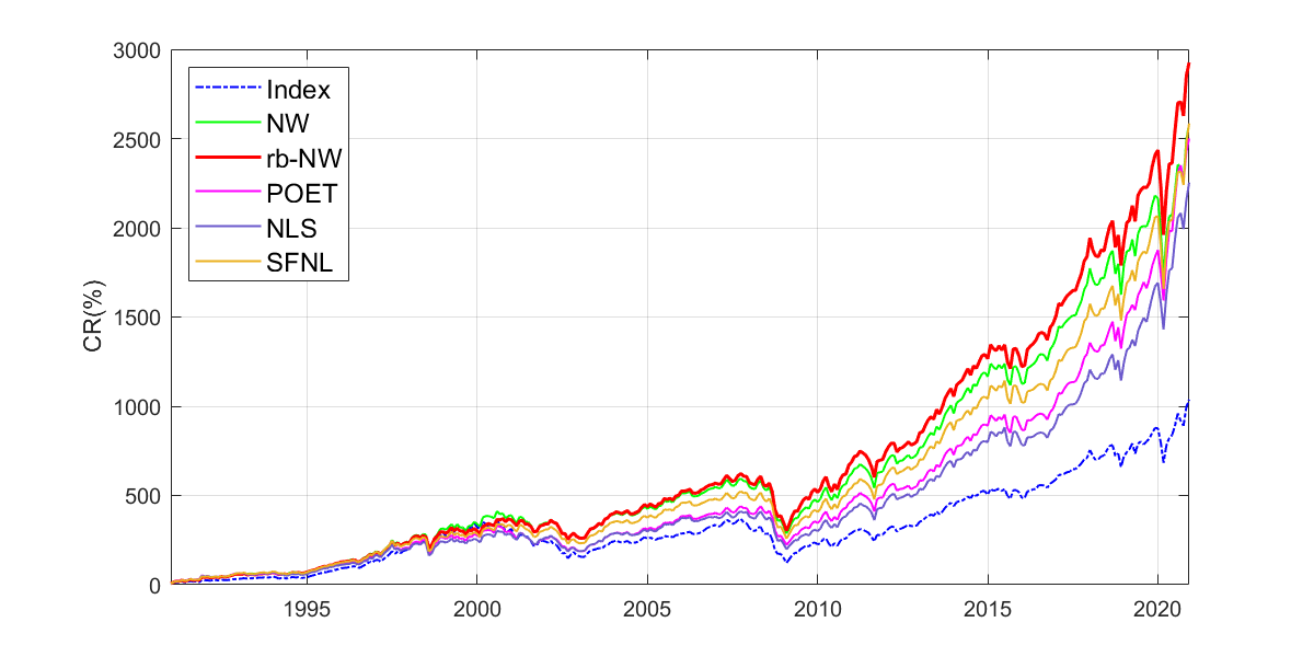
Figure 1: Cumulative excess return of largest 100 stocks in S&P 500 index, out of sample period is 01/1991-12/2020, sample size is 120.

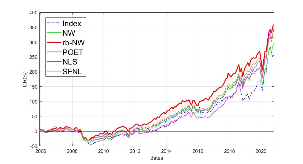
Figure 2: Cumulative excess return of 254 stocks in S&P 500 index, out of sample period is 01/2006-12/2020, sample size is 180.

We also take transaction costs into consideration. Following Ao et al. (2019), the excess portfolio return net of transaction cost is computed as

$$r_{t}^{net}=\left(1-\sum_{i=1}^{p}c\left|\widehat{W}_{t+1,i}-\widehat{W}_{t,i}^{+}\right|\right)(1+r_{t})-1,$$ (13)

where $\widehat{W}_{t+1,i}$ is the $i$-th element of portfolio weight after rebalancing, and $\widehat{W}_{t,i}^{+}$ is the portfolio weight before rebalancing; $r_{t}$ is the excess return of the portfolio without transaction cost and $c$ measures the level of the transaction cost, which is set to 50 basis points. Formally, the portfolio turnover is defined as

$$TO=\frac{1}{RT}\sum_{l=1}^{RT}\sum_{i=1}^{p}\left|\widehat{W}_{l+1,i}-\widehat{W}_{l,i}^{+}\right|,$$ (14)

where $\widehat{W}_{l+1,i}$ is the desired portfolio weight at $(l+1)$-th rebalancing, and $\widehat{W}_{l,i}^{+}$ is portfolio weight before the $(l+1)$-th rebalancing, $RT$ is the number of rebalancing events. The empirical results for scenarios (1) and (2) are reported in Table 8. It shows that the advantages of our proposed portfolio achieved without transaction costs still hold with transaction costs. E.g., the Sharpe ratio of rb-NW portfolio is a bit lower with transaction costs compared to Table 7, but it is still the best among comparison portfolios, and the advantages are more significant when $p>T$. Notice that rb-NW based portfolio gets the lowest turnover ratio, as it has the lowest tracking error to the benchmark index. The p-values of SR test results show that the rb-NW has better SR performance compared to other portfolios when $p<T$, and similar outcome is observed for $p>T$ and monthly performance, at 10% for example.

Table 8: Empirical results for scenarios (1) and (2) with transaction cost.

	Scenario (1): p = 100, T = 120							Scenario (2): p = 254, T = 180
	AVR	TE	Risk	SR	TO	p		AVR	TE	Risk	SR	TO	p
	Monthly
Index	0.0077	-	0.0420	0.1826	-	-		0.0071	-	0.0437	0.1627	-
NW	0.0093	0.0132	0.0423	0.2189	0.1638	0.0032		0.0069	0.0242	0.0439	0.1578	0.3455	0.0029
rb-NW	0.0098	0.0103	0.0407	0.2404	0.1125	-		0.0083	0.0188	0.0406	0.2046	0.2045	-
POET	0.0086	0.0190	0.0419	0.2047	0.2784	0.0026		0.0070	0.0353	0.0433	0.1606	0.4971	0.0862
NLS	0.0082	0.0195	0.0427	0.1932	0.2951	0.0000		0.0072	0.0277	0.0421	0.1704	0.4070	0.0745
SFNL	0.0089	0.0147	0.0420	0.2126	0.2256	0.0017		0.0075	0.0245	0.0418	0.1788	0.3599	0.0894
	Yearly
Index	0.0965	-	0.1713	0.5634	-	-		0.0858	-	0.1729	0.4963	-	-
NW	0.1154	0.0493	0.1617	0.7135	1.9817	0.0380		0.0762	0.0969	0.1596	0.4772	4.2072	0.0220
rb-NW	0.1220	0.0377	0.1595	0.7650	1.3600	-		0.0953	0.0713	0.1528	0.6236	2.4660	-
POET	0.1022	0.0733	0.1657	0.6169	3.3184	0.0170		0.0686	0.1556	0.1589	0.4315	5.9400	0.1610
NLS	0.0980	0.0800	0.1684	0.5817	3.5734	0.0112		0.0755	0.1222	0.1553	0.4860	5.0076	0.1415
SFNL	0.1088	0.0600	0.1603	0.6791	2.7319	0.0345		0.0806	0.1128	0.1526	0.5280	4.3788	0.1807

• TO is the turnover defined in (14). For other measures please see notes in Table 7.

Next, we conduct empirical exercises to study the portfolios with both TE and inequality weight constraints, mimicking the mutual funds focusing on specific sectors (themes). Here, we consider two sectors, the health care sector and the energy sector, and for ease of reporting, we call them scenarios (3) and (4), respectively. Specifically, we select the health care/energy assets from the same S&P 500 assets pool in scenario (2) with 254 stocks, and impose the weight constraint such that our portfolio invests at least 80% of its assets in the themed assets. To compare with TE-only constraint of scenario (2), the out of sample period is set to 01/2006-12/2020 with sample size $T=180$. The benchmark indices for scenarios (3) and (4) are S&P 500 Health Care and S&P 500 Energy, respectively. The results are shown in Table 9. We can observe that the rb-NW based portfolios show overall outstanding performances in average return, risk, and Sharpe ratio. First, the Sharpe ratio of the proposed rb-NW is the best among all portfolios in scenarios (3) and (4). For example, under the ”Yearly” scenario (3), the Sharpe ratio of rb-NW based portfolio is 0.8853, which is higher than the second-ranked POET (0.8227). The shrinkage-based portfolios have outperformed the respective sector indices. We can also compare the themed funds with the market index: from scenario (2) of Table 7, which has the same stocks pool and time period, the market index of S&P 500 has better Sharpe ratio than the energy funds, while the health care funds have higher Sharpe ratio than the market index. Second, the risk of rb-NW portfolios in scenario (3) is the best among all active portfolios and is close to the best (Index) in energy funds. At last, the average returns of rb-NW based portfolios are also the top performer in the two themed funds. We also illustrate the superior returns of rb-NW in Figures 3 and 4, which is consistent with the average returns result in Table 9.

Table 9: Empirical results for scenarios (3) and (4).

	Scenario (3): p = 254, T =180, Health Care						Scenario (4): p = 254, T =180, Energy
	AVR	TE	Risk	SR	p		AVR	TE	Risk	SR	p
	Monthly
Index	0.0079	-	0.0400	0.1988	0.1308		0.0012	-	0.0724	0.0168	0.0165
NW	0.0084	0.0239	0.0414	0.2036	0.0430		0.0045	0.0361	0.0825	0.0546	0.0974
rb-NW	0.0093	0.0128	0.0383	0.2435	-		0.0056	0.0224	0.0768	0.0733	-
POET	0.0091	0.0179	0.0385	0.2376	0.3418		0.0044	0.0494	0.0756	0.0580	0.3873
NLS	0.0084	0.0193	0.0401	0.2096	0.0257		0.0037	0.0362	0.0780	0.0480	0.0873
SFNL	0.0088	0.0172	0.0398	0.2223	0.0885		0.0049	0.0285	0.0778	0.0628	0.3742
	Yearly
Index	0.0973	-	0.1488	0.6543	0.0659		0.0349	-	0.2034	0.1716	0.0433
NW	0.0946	0.0973	0.1353	0.6991	0.0826		0.0360	0.1521	0.2214	0.1628	0.0966
rb-NW	0.1086	0.0501	0.1227	0.8853	-		0.0561	0.0924	0.2020	0.2778	-
POET	0.1049	0.0944	0.1275	0.8227	0.3224		0.0340	0.2534	0.2190	0.1552	0.4280
NLS	0.0925	0.1004	0.1353	0.6834	0.0931		0.0223	0.1934	0.1973	0.1130	0.2268
SFNL	0.0983	0.0969	0.1306	0.7526	0.1807		0.0383	0.1652	0.1858	0.2064	0.4397

• We report the following statistics for portfolio performance evaluations: average returns (AVR), tracking error (TE), standard deviation (Risk), Sharpe ratio (SR) and p-value of the SR test. Scenarios (3) and (4) are themed portfolios (composed of 254 stocks from 01/2006 - 12/2020 from S&P500 index) benchmarking against health care and energy sector, respectively. “-” means the statistic is not available. “Index” means the S&P 500 Health Care and S&P 500 Energy indices, for scenario (3) and (4), respectively. Other portfolios are explained in Table 1 notes.

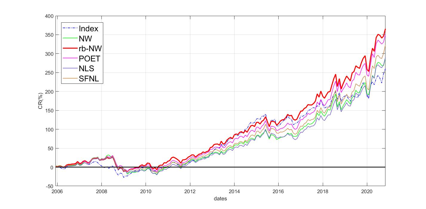
Figure 3: Cumulative excess return of all considered portfolios under scenario (3) (health care sector), out of sample period is 01/2006-12/2020, sample size is 180.

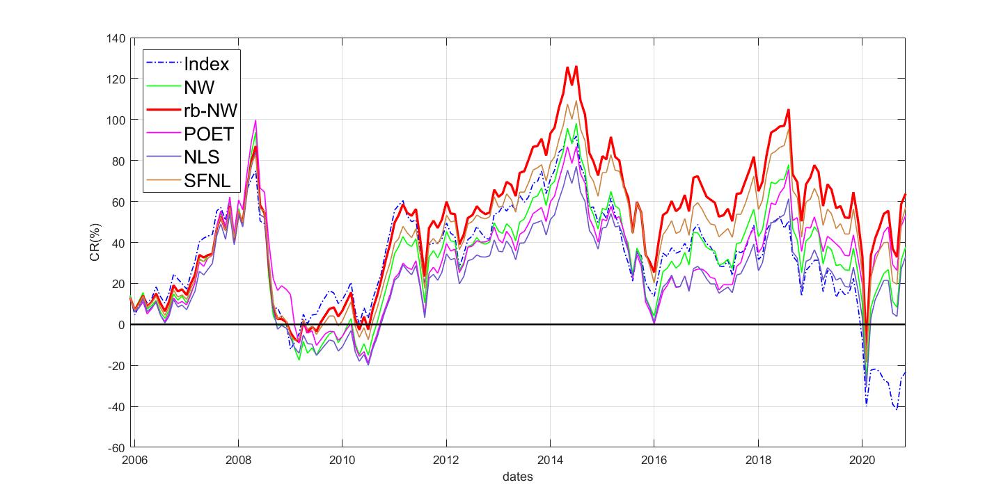
Figure 4: Cumulative excess return of all considered portfolios under scenario (4) (energy sector), out of sample period is 01/2006-12/2020, sample size is 180.

The empirical results for scenarios (3) and (4) with transaction costs are reported in Table 10. It shows that the robustness of the superior performance of the proposed portfolio with transaction costs in the two designated sectors. Same as Table 9, the rb-NW portfolio is still the best performer in health care sector after transaction costs. It has good performance in the energy sector in terms of Sharpe ratio. The results of the SR tests support the better performance of rb-NW in general.

Table 10: Empirical results for scenarios (3) and (4) with transaction cost.

	Scenario (3): p = 254, T =180, Health Care								Scenario (4): p = 254, T =180, Energy
	AVR	TE	Risk	SR	TO	p		AVR	TE	Risk	SR	TO	p
	Monthly
Index	0.0079	-	0.0400	0.1988	-	-		0.0012	-	0.0724	0.0168	-	-
NW	0.0069	0.0241	0.0415	0.1668	0.3038	0.0083		0.0031	0.0291	0.0810	0.0380	0.3929	0.0282
rb-NW	0.0085	0.0129	0.0383	0.2229	0.1570	-		0.0042	0.0225	0.0767	0.0547	0.2870	-
POET	0.0071	0.0180	0.0385	0.1856	0.3983	0.0057		0.0009	0.0373	0.0742	0.0119	0.8448	0.0081
NLS	0.0067	0.0196	0.0401	0.1678	0.3324	0.0011		0.0020	0.0283	0.0772	0.0260	0.5051	0.0056
SFNL	0.0073	0.0174	0.0398	0.1834	0.3081	0.0068		0.0035	0.0213	0.0776	0.0449	0.3977	0.1471
	Yearly
Index	0.0973	-	0.1488	0.6543	-	-		0.0349	-	0.2034	0.1716	-	-
NW	0.0752	0.0975	0.1342	0.5606	3.7668	0.0335		0.0220	0.1237	0.2124	0.1035	4.8096	0.0402
rb-NW	0.0985	0.0507	0.1218	0.8086	1.9368	-		0.0392	0.0938	0.2008	0.1952	3.4476	-
POET	0.0803	0.0938	0.1233	0.6513	4.6104	0.1082		-0.0033	0.1939	0.1930	-0.0171	9.6120	0.0829
NLS	0.0713	0.1013	0.1338	0.5329	4.1316	0.0393		0.0053	0.1545	0.1865	0.0282	6.1596	0.0703
SFNL	0.0785	0.0976	0.1285	0.6108	3.8076	0.0894		0.0254	0.1270	0.1828	0.1387	4.7988	0.1654

• See notes in Table 9.

8 Conclusion

In this paper we develop the first high dimensional constrained portfolio weight estimator by using a new machine learning technique. We prove that our estimator is consistent even when the number of assets are larger than the time span of the portfolio and when the number of factors may grow. We provide rate of convergence results when there are tracking error constraints, or joint tracking error and inequality-equality weight constraints. The future research may look at confidence intervals for Sharpe Ratio of the constrained portfolio.

Appendix

A.1 Proof of Theorem 1(i). See that, with $\boldsymbol{\Theta}\mathrel{\mathop{\mathchar 58\relax}}=\boldsymbol{\Sigma}_{y}^{-1}$, $\hat{\boldsymbol{\Theta}}\mathrel{\mathop{\mathchar 58\relax}}=\hat{\boldsymbol{\Sigma}}_{y}^{-1}$, $\boldsymbol{\Theta}$ is symmetric,

$$\hat{\boldsymbol{w}}_{d}-\boldsymbol{w}_{d}^{*}=\kappa\left[\left(\frac{\hat{\boldsymbol{\Theta}}^{\prime}\hat{\boldsymbol{\mu}}}{\boldsymbol{1}_{p}^{\prime}\hat{\boldsymbol{\Theta}}^{\prime}\hat{\boldsymbol{\mu}}}-\frac{\boldsymbol{\Theta}\boldsymbol{\mu}}{\boldsymbol{1}_{p}^{\prime}\boldsymbol{\Theta}\boldsymbol{\mu}}\right)+\left(\frac{\boldsymbol{\Theta}\boldsymbol{1}_{p}}{\boldsymbol{1}_{p}^{\prime}\boldsymbol{\Theta}\boldsymbol{1}_{p}}-\frac{\hat{\boldsymbol{\Theta}}^{\prime}\boldsymbol{1}_{p}}{\boldsymbol{1}_{p}^{\prime}\hat{\boldsymbol{\Theta}}1_{p}}\right)\right].$$ (A.1)

Define the scalar $A\mathrel{\mathop{\mathchar 58\relax}}=\boldsymbol{1}_{p}^{\prime}\boldsymbol{\Theta}\boldsymbol{1}_{p}/p$, and $\hat{A}\mathrel{\mathop{\mathchar 58\relax}}=\boldsymbol{1}_{p}^{\prime}\hat{\boldsymbol{\Theta}}^{\prime}\boldsymbol{1}_{p}/p$, and consider the following right side term in (A.1)

$$\left\|\frac{\boldsymbol{\Theta}\boldsymbol{1}_{p}}{\boldsymbol{1}_{p}^{\prime}\boldsymbol{\Theta}\boldsymbol{1}_{p}}-\frac{\hat{\boldsymbol{\Theta}}^{\prime}\boldsymbol{1}_{p}}{\boldsymbol{1}_{p}^{\prime}\hat{\boldsymbol{\Theta}}\boldsymbol{1}_{p}}\right\|_{1}=\left\|\frac{\hat{\boldsymbol{\Theta}}^{\prime}\boldsymbol{1}_{p}/p}{\hat{A}}-\frac{\boldsymbol{\Theta}\boldsymbol{1}_{p}/p}{A}\right\|_{1}=\frac{\|(\hat{\boldsymbol{\Theta}}^{\prime}\boldsymbol{1}_{p}/p)A-(\boldsymbol{\Theta}\boldsymbol{1}_{p}/p)\hat{A}\|_{1}}{|\hat{A}A|}$$ (A.2)

We consider the numerator and denominator of (A.2) separately. First see that

$$|\hat{A}A|=|(\hat{A}-A)A+A^{2}|\geq A^{2}-A|\hat{A}-A|.$$ (A.3)

By Assumption 7(ii), $A\geq c>0$ for $c>0$ being a positive constant, and by Lemma B.5 of Caner et al. (2023) $|A|\leq C<\infty$, for a positive constant $C>0$. Then by Assumptions 1-7,

$$|\hat{A}-A| \leq \|\boldsymbol{1}_{p}\|_{\infty}\|(\hat{\boldsymbol{\Theta}}-\boldsymbol{\Theta})^{\prime}\boldsymbol{1}_{p}\|_{1}/p$$ (A.4)

$$\leq \max_{j}\|\hat{\boldsymbol{\Theta}}_{j}-\boldsymbol{\Theta}_{j}\|_{1}$$

$$= O_{p}(\bar{s}l_{T})=o_{p}(1),$$

where $\hat{\boldsymbol{\Theta}}_{j}\mathrel{\mathop{\mathchar 58\relax}}p\times 1$ is the $j$ th row of $\hat{\boldsymbol{\Theta}}$ shown in column format, and for the rate we use Theorem 2(i) of Caner et al. (2023). Combine all those to have

$$|\hat{A}A|\geq c^{2}-o_{p}(1).$$ (A.5)

For the numerator, add and subtract $(\boldsymbol{\Theta}\boldsymbol{1}_{p}/p)A$ in (A.2)

$$\|(\hat{\boldsymbol{\Theta}}^{\prime}\boldsymbol{1}_{p}/p)A-(\boldsymbol{\Theta}\boldsymbol{1}_{p}/p)\hat{A}\|_{1}\leq\frac{1}{p}[\|(\hat{\boldsymbol{\Theta}}-\boldsymbol{\Theta})^{\prime}\boldsymbol{1}_{p}A\|_{1}+\|(\boldsymbol{\Theta}\boldsymbol{1}_{p})(A-\hat{A})\|_{1}],$$ (A.6)

where $\boldsymbol{\Theta}$ is symmetric. Consider each term in (A.6), with $A\geq c>0$

$$\frac{1}{p}\|(\hat{\boldsymbol{\Theta}}-\boldsymbol{\Theta})^{\prime}\boldsymbol{1}_{p}A\|_{1} = A\|(\hat{\boldsymbol{\Theta}}-\boldsymbol{\Theta})^{\prime}\boldsymbol{1}_{p}/p\|_{1}$$

$$\leq A\|(\hat{\boldsymbol{\Theta}}-\boldsymbol{\Theta})^{\prime}\|_{l_{1}}\|\boldsymbol{1}_{p}/p\|_{1}$$

$$= A\|\hat{\boldsymbol{\Theta}}-\boldsymbol{\Theta}\|_{l_{\infty}}$$

$$= A\max_{1\leq j\leq p}\|\hat{\boldsymbol{\Theta}}_{j}-\boldsymbol{\Theta}_{j}\|_{1},$$

where we use p.345 of Horn and Johnson (2013) for the inequality. By Assumptions 1-7, by Theorem 2(i) of Caner et al. (2023)

$$\max_{1\leq j\leq p}\|\hat{\boldsymbol{\Theta}}_{j}-\boldsymbol{\Theta}_{j}\|_{1}=O_{p}(\bar{s}l_{T}).$$ (A.7)

So by Lemma B.5 of Caner et al. (2023) since $|A|\leq C<\infty$

$$\frac{1}{p}\|(\hat{\boldsymbol{\Theta}}-\boldsymbol{\Theta})^{\prime}\boldsymbol{1}_{p}A\|_{1}=O_{p}(\bar{s}l_{T}).$$ (A.8)

Next in (A.6) consider

$$\|(\boldsymbol{\Theta}\boldsymbol{1}_{p}/p)(A-\hat{A})\|_{1}\leq|A-\hat{A}|\|\boldsymbol{\Theta}\boldsymbol{1}_{p}/p\|_{1}\leq|A-\hat{A}|\|\boldsymbol{\Theta}\|_{l_{1}},$$ (A.9)

by p.345 of Horn and Johnson (2013) for the second inequality. Then by symmetry $\|\boldsymbol{\Theta}\|_{l_{1}}=\|\boldsymbol{\Theta}\|_{l_{\infty}}$, with Assumptions 1-7, and defining $\boldsymbol{L}\mathrel{\mathop{\mathchar 58\relax}}=\boldsymbol{B}[({\bf covf_{t}})^{-1}+\boldsymbol{B}^{\prime}\boldsymbol{\Omega}\boldsymbol{B}]^{-1}\boldsymbol{B}^{\prime}$ and use $\boldsymbol{\Theta}\mathrel{\mathop{\mathchar 58\relax}}=\boldsymbol{\Sigma}_{y}^{-1}$ formula in Section 2

$$\|\boldsymbol{\Theta}\|_{l_{\infty}} = \|\boldsymbol{\Omega}-\boldsymbol{\Omega}\boldsymbol{L}\boldsymbol{\Omega}\|_{l_{\infty}}$$ (A.10)

$$\leq \|\boldsymbol{\Omega}\|_{l_{\infty}}+\|\boldsymbol{\Omega}\|_{l_{\infty}}\|\boldsymbol{L}\|_{l_{\infty}}\|\boldsymbol{\Omega}\|_{l_{\infty}}$$

$$= O(\sqrt{\bar{s}})+O(\bar{s}r_{T}K^{3/2})=O(\bar{s}r_{T}K^{3/2}),$$

where the rates are from (A.96)-(A.97) of Caner et al. (2023). Combine (A.9)(A.10) and (A.4)

$$\|(\boldsymbol{\Theta}\boldsymbol{1}_{p}/p)(A-\hat{A})\|_{1}=O_{p}(\bar{s}r_{T}K^{3/2})O_{p}(\bar{s}l_{T})=O_{p}(\bar{s}^{2}l_{T}r_{T}K^{3/2}).$$ (A.11)

Combine rates (A.8)(A.11), and clearly (A.11) is slower so the rate in (A.6) is

$$\|(\hat{\boldsymbol{\Theta}}^{\prime}\boldsymbol{1}_{p}/p)A-(\boldsymbol{\Theta}\boldsymbol{1}_{p}/p)\hat{A}\|_{1}=O_{p}(\bar{s}^{2}l_{T}r_{T}K^{3/2}).$$ (A.12)

Then by (A.5)(A.12) in (A.2)

$$\frac{\|(\hat{\boldsymbol{\Theta}}^{\prime}\boldsymbol{1}_{p}/p)A-(\boldsymbol{\Theta}\boldsymbol{1}_{p}/p)\hat{A}\|_{1}}{|\hat{A}A|}=O_{p}(\bar{s}^{2}l_{T}r_{T}K^{3/2})=o_{p}(1),$$ (A.13)

by Assumption 7(i), $\bar{s}^{2}l_{T}r_{T}K^{3/2}=o(1)$. Define scalar $F\mathrel{\mathop{\mathchar 58\relax}}=\boldsymbol{1}_{p}^{\prime}\boldsymbol{\Theta}\boldsymbol{\mu}/p$, and $\hat{F}\mathrel{\mathop{\mathchar 58\relax}}=\boldsymbol{1}_{p}^{\prime}\hat{\boldsymbol{\Theta}}^{\prime}\hat{\boldsymbol{\mu}}/p$ on right side term in (A.1)

$$\left\|\left(\frac{\hat{\boldsymbol{\Theta}}^{\prime}\hat{\boldsymbol{\mu}}}{\boldsymbol{1}_{p}^{\prime}\hat{\boldsymbol{\Theta}}^{\prime}\hat{\boldsymbol{\mu}}}-\frac{\boldsymbol{\Theta}\boldsymbol{\mu}}{\boldsymbol{1}_{p}^{\prime}\boldsymbol{\Theta}\boldsymbol{\mu}}\right)\right\|_{1}=\frac{\|(\hat{\boldsymbol{\Theta}}^{\prime}\hat{\boldsymbol{\mu}}/p)F-(\boldsymbol{\Theta}\boldsymbol{\mu}/p)\hat{F}\|_{1}}{|F\hat{F}|}.$$ (A.14)

In (A.14) consider the denominator first

$$|F\hat{F}|\geq F^{2}-|\hat{F}-F|,$$

with the same analysis in (A.3). Then under Assumptions 1-7(i)

$$|\hat{F}-F|=O_{p}(K\bar{s}l_{T})=o_{p}(1).$$ (A.15)

We prove (A.15) now. First, consider the following term

$$|\boldsymbol{1}_{p}^{\prime}(\hat{\boldsymbol{\Theta}}-\boldsymbol{\Theta})^{\prime}(\hat{\boldsymbol{\mu}}-\boldsymbol{\mu})|/p \leq \|\boldsymbol{1}_{p}^{\prime}(\hat{\boldsymbol{\Theta}}-\boldsymbol{\Theta})^{\prime}\|_{1}\|(\hat{\boldsymbol{\mu}}-\boldsymbol{\mu})\|_{\infty}/p$$ (A.16)

$$\leq (\|\boldsymbol{1}_{p}\|_{1}/p)\|(\hat{\boldsymbol{\Theta}}-\boldsymbol{\Theta})^{\prime}\|_{l_{1}}\|(\hat{\boldsymbol{\mu}}-\boldsymbol{\mu})\|_{\infty},$$

where we use Holder’s inequality for the first inequality, and p.345 of Horn and Johnson (2013) for the second inequality. Note that $\boldsymbol{\Theta}$ is symmetric

$$\left|\frac{\boldsymbol{1}_{p}^{\prime}\hat{\boldsymbol{\Theta}}^{\prime}\hat{\boldsymbol{\mu}}}{p}-\frac{\boldsymbol{1}_{p}^{\prime}\boldsymbol{\Theta}^{\prime}\boldsymbol{\mu}}{p}\right| \leq \frac{1}{p}\left|\boldsymbol{1}_{p}^{\prime}(\hat{\boldsymbol{\Theta}}-\boldsymbol{\Theta})^{\prime}(\hat{\boldsymbol{\mu}}-\boldsymbol{\mu})\right|+\frac{1}{p}\left|\boldsymbol{1}_{p}(\hat{\boldsymbol{\Theta}}-\boldsymbol{\Theta})^{\prime}\boldsymbol{\mu}\right|+\frac{1}{p}\left|\boldsymbol{1}_{p}^{\prime}\boldsymbol{\Theta}^{\prime}(\hat{\boldsymbol{\mu}}-\boldsymbol{\mu})\right|$$

$$= O_{p}(\bar{s}l_{T})O_{p}(max(K\frac{\sqrt{lnT}}{\sqrt{T}},\frac{\sqrt{lnp}}{\sqrt{T}}))+O_{p}(\bar{s}l_{T})O(K)$$

$$+ O_{p}(\bar{s}r_{T}K^{3/2})O_{p}(max(K\frac{\sqrt{lnT}}{\sqrt{T}},\frac{\sqrt{lnp}}{\sqrt{T}}))$$

$$= O_{p}(\bar{s}l_{T}K),$$

where we use (A.16) and the same technical analysis in (A.4), and the rates are from (A.7) here and then Theorem 2(ii) of Caner et al. (2023) for the first term on the right side, and for the second term rates are by (A.7) here and then (B.8) of Caner et al. (2023), and for the third term, rates are by (A.10) here and $\|\boldsymbol{\Theta}^{\prime}\|_{l_{1}}=\|\boldsymbol{\Theta}\|_{l_{\infty}}$, and Theorem 2(ii) of Caner et al. (2023). Second rate is the slowest by $l_{T}$ definition in (2).

By Lemma B.5 of Caner et al. (2023)

$$|F|=O(K^{1/2}),$$

and by the condition $|F|\geq c>0$, we have by Assumption 7

$$|F\hat{F}|\geq c^{2}-o_{p}(1).$$ (A.17)

Now consider the numerator in (A.14), by adding and subtracting $(\boldsymbol{\Theta}\boldsymbol{\mu}/p)F$ and triangle inequality

$$\|\frac{\hat{\boldsymbol{\Theta}}^{\prime}\hat{\boldsymbol{\mu}}}{p}F-\frac{\boldsymbol{\Theta}\boldsymbol{\mu}}{p}\hat{F}\|_{1}\leq\|\frac{\hat{\boldsymbol{\Theta}}^{\prime}\hat{\boldsymbol{\mu}}}{p}F-\frac{\boldsymbol{\Theta}\boldsymbol{\mu}}{p}F\|_{1}+\|\frac{\boldsymbol{\Theta}\boldsymbol{\mu}}{p}(\hat{F}-F)\|_{1}.$$ (A.18)

In (A.18) by adding and subtracting, $\boldsymbol{\Theta}$ being symmetric

$$\hat{\boldsymbol{\Theta}}^{\prime}\hat{\boldsymbol{\mu}}-\boldsymbol{\Theta}\boldsymbol{\mu}=(\hat{\boldsymbol{\Theta}}-\boldsymbol{\Theta})^{\prime}\hat{\boldsymbol{\mu}}+\boldsymbol{\Theta}(\hat{\boldsymbol{\mu}}-\boldsymbol{\mu}).$$ (A.19)

Use the first term on the right side above

$$\frac{1}{p}\|(\hat{\boldsymbol{\Theta}}-\boldsymbol{\Theta})^{\prime}\hat{\boldsymbol{\mu}}\|_{1} \leq \frac{1}{p}\|(\hat{\boldsymbol{\Theta}}-\boldsymbol{\Theta})^{\prime}\|_{l_{1}}\|\hat{\boldsymbol{\mu}}\|_{1}$$ (A.20)

$$\leq \|\hat{\boldsymbol{\Theta}}-\boldsymbol{\Theta}\|_{l_{\infty}}\|\hat{\boldsymbol{\mu}}\|_{\infty}=O_{p}(\bar{s}l_{T})O_{p}(K),$$

where we use p.345 of Horn and Johnson (2013) for the first inequality and for the rates, we use Theorem 2 of Caner et al. (2023) and (B.8) of Caner et al. (2023) by Assumptions 1-7. Now consider the second term on the right side of (A.19)

$$\frac{1}{p}\|\boldsymbol{\Theta}(\hat{\boldsymbol{\mu}}-\boldsymbol{\mu})\|_{1} \leq \|\boldsymbol{\Theta}\|_{l_{1}}\|\hat{\boldsymbol{\mu}}-\boldsymbol{\mu}\|_{\infty}$$ (A.21)

$$= \|\boldsymbol{\Theta}\|_{l_{\infty}}\|\hat{\boldsymbol{\mu}}-\boldsymbol{\mu}\|_{\infty}=O(\bar{s}r_{T}K^{3/2})O_{p}(max(K\sqrt{\frac{lnT}{T}},\sqrt{\frac{lnp}{T}})))$$

where we use the same analysis as in (A.20) for the inequality, and the rates are by (A.10) here and Theorem 2(ii)of Caner et al. (2023). Then (A.20) is slower as a rate than in (A.21) due to $l_{T}$ definition in(2). So with $|F|=O(\sqrt{K})$ by Lemma B.5 of Caner et al. (2023), in (A.18) the first right side term is

$$\|\frac{\hat{\boldsymbol{\Theta}}^{\prime}\hat{\boldsymbol{\mu}}}{p}-\frac{\boldsymbol{\Theta}\boldsymbol{\mu}}{p}\|_{1}|F|=O_{p}(\bar{s}l_{T}K^{3/2}).$$ (A.22)

Next in (A.18), the second right side term is

$$\|\frac{\boldsymbol{\Theta}\boldsymbol{\mu}}{p}(\hat{F}-F)\|_{1} = \|\frac{\boldsymbol{\Theta}\boldsymbol{\mu}}{p}\|_{1}|\hat{F}-F|$$ (A.23)

$$\leq \|\boldsymbol{\Theta}\|_{l_{1}}\|\boldsymbol{\mu}\|_{\infty}|\hat{F}-F|$$

$$= \|\boldsymbol{\Theta}\|_{l_{\infty}}\|\boldsymbol{\mu}\|_{\infty}|\hat{F}-F|$$

$$= O_{p}(\bar{s}r_{T}K^{3/2})O(K)O_{p}(K\bar{s}l_{T}),$$

where we use p.345 of Horn and Johnson (2013) and $\|\mu\|_{1}\leq p\|\mu\|_{\infty}$ for the first inequality, and the rates are by (A.10) here, and then by (B.8) of Caner et al. (2023) which is $\|\mu\|_{\infty}=O(K)$ and (A.15). Clearly the rate in (A.23) is slower than the one in (A.22), so (A.18)

$$\|\frac{\hat{\boldsymbol{\Theta}}^{\prime}\hat{\boldsymbol{\mu}}}{p}F-\frac{\boldsymbol{\Theta}\boldsymbol{\mu}}{p}\hat{F}\|_{1}=O_{p}(\bar{s}^{2}l_{T}r_{T}K^{7/2}).$$ (A.24)

Use (A.24)(A.17) in (A.14) to have

$$\left\|\left(\frac{\hat{\boldsymbol{\Theta}}^{\prime}\hat{\boldsymbol{\mu}}}{1_{p}^{\prime}\hat{\boldsymbol{\Theta}}^{\prime}\hat{\boldsymbol{\mu}}}-\frac{\boldsymbol{\Theta}\boldsymbol{\mu}}{\boldsymbol{1}_{p}^{\prime}\boldsymbol{\Theta}\boldsymbol{\mu}}\right)\right\|_{1}=O_{p}(\bar{s}^{2}l_{T}r_{T}K^{7/2})=o_{p}(1),$$ (A.25)

by Assumption 7(i) to have the last equality. Use (A.13)(A.24) in the weights definition in (A.1)

$$\|\hat{\boldsymbol{w}}_{d}-\boldsymbol{w}_{d}^{*}\|_{1}=O_{p}(\bar{s}^{2}l_{T}r_{T}K^{7/2})=o_{p}(1)$$

.Q.E.D.

Proof of Theorem 1(ii). The difference between the out-of sample large portfolio variance estimate and its theoretical counterpart is:

$$\hat{\boldsymbol{w}}^{\prime}\boldsymbol{\Sigma}_{y}\hat{\boldsymbol{w}}-\boldsymbol{w}^{*^{\prime}}\boldsymbol{\Sigma}_{y}\boldsymbol{w}^{*}.$$

Note that $\boldsymbol{w}^{*}=\boldsymbol{w}_{d}^{*}+\boldsymbol{m}$, and $\hat{\boldsymbol{w}}=\hat{\boldsymbol{w}}_{d}+\boldsymbol{m}$. We can simplify

$$\hat{\boldsymbol{w}}^{\prime}\boldsymbol{\Sigma}_{y}\hat{\boldsymbol{w}}-\boldsymbol{w}^{*^{\prime}}\boldsymbol{\Sigma}_{y}\boldsymbol{w}^{*}=(\hat{\boldsymbol{w}}_{d}^{\prime}\boldsymbol{\Sigma}_{y}\hat{\boldsymbol{w}}_{d}-\boldsymbol{w}_{d}^{*^{\prime}}\boldsymbol{\Sigma}_{y}\boldsymbol{w}_{d}^{*})+2\boldsymbol{m}^{\prime}\boldsymbol{\Sigma}_{y}(\hat{\boldsymbol{w}}_{d}-\boldsymbol{w}_{d}).$$ (A.26)

We consider each term in (A.26). First,

$$(\hat{\boldsymbol{w}}_{d}^{\prime}\boldsymbol{\Sigma}_{y}\hat{\boldsymbol{w}}_{d}-\boldsymbol{w}_{d}^{*^{\prime}}\boldsymbol{\Sigma}_{y}\boldsymbol{w}_{d}^{*})=(\hat{\boldsymbol{w}}_{d}-\boldsymbol{w}_{d}^{*})^{\prime}\boldsymbol{\Sigma}_{y}(\hat{\boldsymbol{w}}_{d}-\boldsymbol{w}_{d}^{*})+2\boldsymbol{w}_{d}^{*^{\prime}}\boldsymbol{\Sigma}_{y}(\hat{\boldsymbol{w}}_{d}-\boldsymbol{w}_{d}^{*}).$$ (A.27)

Before the analysis of two terms on the right side of (A.27), we see

$$\|\boldsymbol{\Sigma}_{y}\|_{\infty} \leq \|\boldsymbol{B}{\bf covf_{t}}\boldsymbol{B}^{\prime}\|_{\infty}+\|\boldsymbol{\Sigma}_{u}\|_{\infty}$$ (A.28)

$$\leq K^{2}\|\boldsymbol{B}\|_{\infty}^{2}\|{\bf covf_{t}}\|_{\infty}+\|\boldsymbol{\Sigma}_{u}\|_{\infty}=O(K^{2}),$$

where we obtain the second inequality using Lemma A.1(ii) of Caner et al. (2023) which is $\|\boldsymbol{A}_{1}\boldsymbol{B}_{1}\boldsymbol{A}_{1}^{\prime}\|_{\infty}\leq K^{2}\|\boldsymbol{A}_{1}\|_{\infty}\|\boldsymbol{B}_{1}\|_{\infty}$, where $\boldsymbol{A}_{1}\mathrel{\mathop{\mathchar 58\relax}}p\times K$ matrix, $\boldsymbol{B}_{1}\mathrel{\mathop{\mathchar 58\relax}}K\times K$ matrix, and the rates are by Assumption 1, 4, 5(i).

Consider each term in (A.27), and see that by Holder’s inequality, and $\|\boldsymbol{A}\boldsymbol{x}\|_{\infty}\leq\|\boldsymbol{A}\|_{\infty}\|\boldsymbol{x}\|_{1}$ for generic $\boldsymbol{A},\boldsymbol{x}$ matrix-vector pair,

$$(\hat{\boldsymbol{w}}_{d}-\boldsymbol{w}_{d}^{*})^{\prime}\boldsymbol{\Sigma}_{y}(\hat{\boldsymbol{w}}_{d}-\boldsymbol{w}_{d}^{*}) \leq \|\hat{\boldsymbol{w}}_{d}-\boldsymbol{w}_{d}^{*}\|_{1}\|\boldsymbol{\Sigma}_{y}(\hat{\boldsymbol{w}}_{d}-\boldsymbol{w}_{d}^{*})\|_{\infty}$$ (A.29)

$$\leq \|\hat{\boldsymbol{w}}_{d}-\boldsymbol{w}_{d}^{*}\|_{1}^{2}\|\boldsymbol{\Sigma}_{y}\|_{\infty}$$

$$= O_{p}(r_{w1}^{2})O(K^{2}),$$

where we use Theorem 1(i), since $r_{w1}$ is the rate of convergence in Theorem 1(i), and (A.28).

Before considering second right side term in (A.27), we analyze $l_{1}$ norm of $w_{d}^{*}$.

$$\|\boldsymbol{w}_{d}^{*}\|_{1}=|\kappa|\|\frac{\boldsymbol{\Theta}\boldsymbol{\mu}}{\boldsymbol{1}_{p}^{\prime}\boldsymbol{\Theta}\boldsymbol{\mu}}-\frac{\boldsymbol{\Theta}\boldsymbol{1}_{p}}{\boldsymbol{1}_{p}^{\prime}\boldsymbol{\Theta}\boldsymbol{1}_{p}}\|_{1}.$$ (A.30)

In (A.30)

$$\|\frac{\boldsymbol{\Theta}\boldsymbol{\mu}}{\boldsymbol{1}_{p}^{\prime}\boldsymbol{\Theta}\boldsymbol{\mu}}-\frac{\boldsymbol{\Theta}\boldsymbol{1}_{p}}{\boldsymbol{1}_{p}^{\prime}\boldsymbol{\Theta}1_{p}}\|_{1}\leq\|\frac{\boldsymbol{\Theta}\boldsymbol{\mu}/p}{\boldsymbol{1}_{p}^{\prime}\boldsymbol{\Theta}\boldsymbol{\mu}/p}\|_{1}+\|\frac{\boldsymbol{\Theta}\boldsymbol{1}_{p}/p}{\boldsymbol{1}_{p}^{\prime}\boldsymbol{\Theta}\boldsymbol{1}_{p}/p}\|_{1}.$$ (A.31)

First we consider the denominators in (A.31). By Assumption 7(ii) and $|\boldsymbol{1}_{p}^{\prime}\boldsymbol{\Theta}\boldsymbol{\mu}|/p\geq c>0$ in the statement of Theorem 1, denominators are bounded away from zero. For the numerators in (A.31), now see that $\boldsymbol{\Theta}$ is symmetric, and by (A.10), with p.345 of Horn and Johnson (2013), and by (B.8) of Caner et al. (2023) since $\|\boldsymbol{\mu}\|_{\infty}=O(K)$

$$\|\boldsymbol{\Theta}\boldsymbol{\mu}/p\|_{1} \leq \frac{1}{p}\|\boldsymbol{\Theta}\|_{l_{1}}\|\boldsymbol{\mu}\|_{1}$$ (A.32)

$$\leq \|\boldsymbol{\Theta}\|_{l_{\infty}}\|\boldsymbol{\mu}\|_{\infty}=O(\bar{s}r_{T}K^{3/2})O(K)=O(\bar{s}r_{T}K^{5/2}).$$

In the same way as (A.32)

$$\|\boldsymbol{\Theta}\boldsymbol{1}_{p}/p\|_{1}=O(\bar{s}r_{T}K^{3/2}).$$ (A.33)

Clearly by (A.32)(A.33) into (A.30), and since $\kappa$ is a constant,

$$\|\boldsymbol{w}_{d}^{*}\|_{1}=O(\bar{s}r_{T}K^{5/2}).$$ (A.34)

Clearly we have growing exposure case in the weights differenced from the benchmark. See that the second right side term in (A.27) can be upper bounded as , by Holder’s inequality,

$$|\boldsymbol{w}_{d}^{*^{\prime}}\boldsymbol{\Sigma}_{y}(\hat{\boldsymbol{w}}_{d}-\boldsymbol{w}_{d}^{*})| \leq \|\boldsymbol{w}_{d}^{*}\|_{1}\|\boldsymbol{\Sigma}_{y}(\hat{\boldsymbol{w}}_{d}-\boldsymbol{w}_{d}^{*})\|_{\infty}$$ (A.35)

$$\leq \|\boldsymbol{w}_{d}^{*}\|_{1}\|\boldsymbol{\Sigma}_{y}\|_{\infty}\|\hat{\boldsymbol{w}}_{d}-\boldsymbol{w}_{d}^{*}\|_{1},$$

where we use $\|\boldsymbol{A}\boldsymbol{x}\|_{\infty}\leq\|\boldsymbol{A}\|_{\infty}\|\boldsymbol{x}\|_{1}$ for generic matrix $\boldsymbol{A}$ and generic vector $\boldsymbol{x}$.

Combine Theorem 1(i), (A.28)(A.34) in (A.35) to have

$$|\boldsymbol{w}_{d}^{*^{\prime}}\boldsymbol{\Sigma}_{y}(\hat{\boldsymbol{w}}_{d}-\boldsymbol{w}_{d}^{*})|=O_{p}(r_{w1}\bar{s}r_{T}K^{9/2})=o_{p}(1),$$ (A.36)

by Assumption 7. Combine (A.29)(A.36) in (A.27) to have

$$|\hat{\boldsymbol{w}}_{d}^{\prime}\boldsymbol{\Sigma}_{y}\hat{\boldsymbol{w}}_{d}-\boldsymbol{w}_{d}^{*^{\prime}}\boldsymbol{\Sigma}_{y}\boldsymbol{w}_{d}^{*}|=O_{p}(r_{w1}\bar{s}r_{T}K^{9/2})=o_{p}(1),$$ (A.37)

by $r_{w1}$ rate definition and Assumption 7(i). Since we assume $\|\boldsymbol{m}\|_{1}=O(\|w_{d}^{*}\|_{1})$, we have

$$|\boldsymbol{m}^{\prime}\boldsymbol{\Sigma}_{y}(\hat{\boldsymbol{w}}_{d}-\boldsymbol{w}_{d}^{*})|=O_{p}(r_{w1}\bar{s}r_{T}K^{9/2})=o_{p}(1),$$ (A.38)

where we use exactly the same analysis in (A.36). Next combine (A.37)(A.38) in (A.26), and Assumption 7(iii) to have the desired result.Q.E.D

Proof of Theorem 1(iii). Note that

$$\left[\frac{\widehat{SR}}{SR}\right]^{2}-1=\frac{[(\frac{\hat{\boldsymbol{w}}^{\prime}\boldsymbol{\mu})^{2}}{\hat{\boldsymbol{w}}^{\prime}\boldsymbol{\Sigma}_{y}\hat{\boldsymbol{w}}}]}{[\frac{(\boldsymbol{w}^{*^{\prime}}\boldsymbol{\mu})^{2}}{\boldsymbol{w}^{*^{\prime}}\boldsymbol{\Sigma}_{y}\boldsymbol{w}^{*}}]}-1=\left(\frac{(\hat{\boldsymbol{w}}^{\prime}\boldsymbol{\mu})^{2}}{(\boldsymbol{w}^{*^{\prime}}\boldsymbol{\mu})^{2}}\right)\left(\frac{\boldsymbol{w}^{*^{\prime}}\boldsymbol{\Sigma}_{y}\boldsymbol{w}^{*}}{\hat{\boldsymbol{w}}^{\prime}\boldsymbol{\Sigma}_{y}\hat{\boldsymbol{w}}}\right)-1.$$

Next by adding and subtracting one from each term on the right side of the expression above

$$\left[\frac{\widehat{SR}}{SR}\right]^{2}-1=\left[\frac{(\hat{\boldsymbol{w}}^{\prime}\boldsymbol{\mu})^{2}-(\boldsymbol{w}^{*^{\prime}}\boldsymbol{\mu})^{2}}{(\boldsymbol{w}^{*^{\prime}}\boldsymbol{\mu})^{2}}+1\right]\left[\frac{\boldsymbol{w}^{*^{\prime}}\boldsymbol{\Sigma}_{y}\boldsymbol{w}^{*}-\hat{\boldsymbol{w}}^{\prime}\boldsymbol{\Sigma}_{y}\hat{\boldsymbol{w}}}{\hat{\boldsymbol{w}}^{\prime}\boldsymbol{\Sigma}_{y}\hat{\boldsymbol{w}}}+1\right]-1.$$

Clearly we can simplify the right side above

$$\left|\left[\frac{\widehat{SR}}{SR}\right]^{2}-1\right| \leq \left|\frac{(\hat{\boldsymbol{w}}^{\prime}\boldsymbol{\mu})^{2}-(\boldsymbol{w}^{*^{\prime}}\boldsymbol{\mu})^{2}}{(\boldsymbol{w}^{*^{\prime}}\boldsymbol{\mu})^{2}}\right|\left|\frac{\boldsymbol{w}^{*^{\prime}}\boldsymbol{\Sigma}_{y}\boldsymbol{w}^{*}-\hat{\boldsymbol{w}}^{\prime}\boldsymbol{\Sigma}_{y}\hat{\boldsymbol{w}}}{\hat{\boldsymbol{w}}^{\prime}\boldsymbol{\Sigma}_{y}\hat{\boldsymbol{w}}}\right|$$ (A.39)

$$+ \left|\frac{(\hat{\boldsymbol{w}}^{\prime}\boldsymbol{\mu})^{2}-(\boldsymbol{w}^{*^{\prime}}\boldsymbol{\mu})^{2}}{(\boldsymbol{w}^{*^{\prime}}\boldsymbol{\mu})^{2}}\right|+\left|\frac{\boldsymbol{w}^{*^{\prime}}\boldsymbol{\Sigma}_{y}\boldsymbol{w}^{*}-\hat{\boldsymbol{w}}^{\prime}\boldsymbol{\Sigma}_{y}\hat{\boldsymbol{w}}}{\hat{\boldsymbol{w}}^{\prime}\boldsymbol{\Sigma}_{y}\hat{\boldsymbol{w}}}\right|.$$

Note that

$$\frac{|(\hat{\boldsymbol{w}}^{\prime}\boldsymbol{\mu})^{2}-(\boldsymbol{w}^{*^{\prime}}\boldsymbol{\mu})^{2}|}{(\boldsymbol{w}^{*^{\prime}}\boldsymbol{\mu})^{2}}=\frac{|[(\hat{\boldsymbol{w}}+\boldsymbol{w}^{*})^{\prime}\boldsymbol{\mu}][(\hat{\boldsymbol{w}}-\boldsymbol{w}^{*})^{\prime}\boldsymbol{\mu}]|}{(\boldsymbol{w}^{*^{\prime}}\boldsymbol{\mu})^{2}}.$$ (A.40)

Next,

$$|(\hat{\boldsymbol{w}}+\boldsymbol{w}^{*})^{\prime}\boldsymbol{\mu}| \leq \|\hat{\boldsymbol{w}}+\boldsymbol{w}^{*}\|_{1}\|\boldsymbol{\mu}\|_{\infty}$$ (A.41)

$$= \|\hat{\boldsymbol{w}}-\boldsymbol{w}^{*}+\boldsymbol{w}^{*}+\boldsymbol{w}^{*}\|_{1}\|\boldsymbol{\mu}\|_{\infty}$$

$$\leq \|\hat{\boldsymbol{w}}-\boldsymbol{w}^{*}\|_{1}\|\boldsymbol{\mu}\|_{\infty}+2\|\boldsymbol{w}^{*}\|_{1}\|\boldsymbol{\mu}\|_{\infty}$$

$$= O_{p}(r_{w1}K)+O(\bar{s}r_{T}K^{7/2})=o_{p}(1)+O(\bar{s}r_{T}K^{7/2})=O_{p}(\bar{s}r_{T}K^{7/2}),$$

where for the first inequality we use Holder’s, and then the second inequality is by triangle inequality, for the rates we use Theorem 1(i) here and (B.8) of Caner et al. (2023) in which $\|\boldsymbol{\mu}\|_{\infty}=O(K)$, and $\boldsymbol{w}^{*}\mathrel{\mathop{\mathchar 58\relax}}=\boldsymbol{w}_{d}^{*}+\boldsymbol{m}$, (A.34), Assumption 7(iv), and the last rate is by Assumption 7(i) with $r_{w1}=o(1)$ definition.

First consider, by Theorem 1(ii), and Holder’s inequality, and by assuming $|\boldsymbol{w}^{*^{\prime}}\boldsymbol{\mu}|\geq c>0$, and (B.8) of Caner et al. (2023)

$$\frac{|\hat{\boldsymbol{w}}^{\prime}\boldsymbol{\mu}-\boldsymbol{w}^{*^{\prime}}\boldsymbol{\mu}|}{(\boldsymbol{w}^{*^{\prime}}\boldsymbol{\mu})^{2}}\leq\frac{\|\hat{\boldsymbol{w}}-\boldsymbol{w}^{*}\|_{1}\|\boldsymbol{\mu}\|_{\infty}}{(\boldsymbol{w}^{*^{\prime}}\boldsymbol{\mu})^{2}}=O_{p}(r_{w1}K).$$ (A.42)

So combine (A.41)(A.42) with (A.40)

$$\frac{|(\hat{\boldsymbol{w}}^{\prime}\boldsymbol{\mu})^{2}-(\boldsymbol{w}^{*^{\prime}}\boldsymbol{\mu})^{2}|}{(\boldsymbol{w}^{*^{\prime}}\boldsymbol{\mu})^{2}}=O_{p}(r_{w1}K)O_{p}(\bar{s}r_{T}K^{7/2})=O_{p}(\bar{s}^{3}r_{T}^{2}l_{T}K^{8})=o_{p}(1),$$ (A.43)

by Assumption 7(i) and $r_{w1}$ definition in Theorem 1(i).

Then

$$\left|\frac{\boldsymbol{w}^{*^{\prime}}\boldsymbol{\Sigma}_{y}\boldsymbol{w}^{*}-\hat{\boldsymbol{w}}^{\prime}\boldsymbol{\Sigma}_{y}\hat{\boldsymbol{w}}}{\hat{\boldsymbol{w}}^{\prime}\boldsymbol{\Sigma}_{y}\hat{\boldsymbol{w}}}\right| \leq \left|\frac{\boldsymbol{w}^{*^{\prime}}\boldsymbol{\Sigma}_{y}\boldsymbol{w}^{*}-\hat{\boldsymbol{w}}^{\prime}\boldsymbol{\Sigma}_{y}\hat{\boldsymbol{w}}}{\boldsymbol{w}^{*^{\prime}}\boldsymbol{\Sigma}_{y}\boldsymbol{w}^{*}-|\hat{\boldsymbol{w}}^{\prime}\boldsymbol{\Sigma}_{y}\hat{\boldsymbol{w}}-\boldsymbol{w}^{*^{\prime}}\boldsymbol{\Sigma}_{y}\boldsymbol{w}^{*}|}\right|$$ (A.44)

$$= O_{p}(r_{w1}\bar{s}r_{T}K^{9/2})=O_{p}(\bar{s}^{3}r_{T}^{2}l_{T}K^{8}),$$

by Theorem 1(ii) proof. Use (A.43)(A.44) in (A.39) to have the desired result. Q.E.D.

A.2 Relation Between Tracking Error and Risk Aversion

Here we provide the relation between $TE$ and risk aversion parameter $\Xi$.

$TE\geq\sqrt{(\boldsymbol{w}^{*}-\boldsymbol{m})^{\prime}\boldsymbol{\Sigma}_{y}(\boldsymbol{w}^{*}-\boldsymbol{m})}=\sqrt{\boldsymbol{w}_{d}^{*\prime}\boldsymbol{\Sigma}_{y}\boldsymbol{w}_{d}^{*}}$. From equations (1)-(5) of Bajeux-Besnainou et al. (2011) we have, $\boldsymbol{\Theta}\mathrel{\mathop{\mathchar 58\relax}}=\boldsymbol{\Sigma}_{y}^{-1}$:

$$\boldsymbol{w}_{d}^{*}=\frac{{\boldsymbol{1}_{p}}^{\prime}\boldsymbol{\Theta}\boldsymbol{\mu}}{\Xi}\left(\frac{\boldsymbol{\Theta}\boldsymbol{\mu}}{{\boldsymbol{1}_{p}}^{\prime}\boldsymbol{\Theta}\boldsymbol{\mu}}-\frac{\boldsymbol{\Theta}{\boldsymbol{1}_{p}}}{{\boldsymbol{1}_{p}}^{\prime}\boldsymbol{\Theta}\boldsymbol{1}_{p}}\right)=\frac{1}{\Xi}\left(\boldsymbol{\Theta}\boldsymbol{\mu}-\frac{{\boldsymbol{1}_{p}}^{\prime}\boldsymbol{\Theta}\boldsymbol{\mu}}{{\boldsymbol{1}_{p}}^{\prime}\boldsymbol{\Theta}{\boldsymbol{1}_{p}}}\cdot\boldsymbol{\Theta}{\boldsymbol{1}_{p}}\right)$$

Define $\delta=\frac{{\boldsymbol{1}_{p}}^{\prime}\boldsymbol{\Theta}\boldsymbol{\mu}}{{\boldsymbol{1}_{p}}^{\prime}\boldsymbol{\Theta}{\boldsymbol{1}_{p}}}$, then $\boldsymbol{w}_{d}^{*}=\frac{\boldsymbol{\Theta}}{\Xi}(\boldsymbol{\mu}-\delta{\boldsymbol{1}_{p}})$. Now we plug in $TE$ and by symmetry of $\boldsymbol{\Theta}$

$$TE \geq\sqrt{\boldsymbol{w}_{d}^{*\prime}\boldsymbol{\Sigma}_{y}\boldsymbol{w}_{d}^{*}}=\sqrt{\frac{1}{\Xi}\cdot(\boldsymbol{\mu}-\delta{\boldsymbol{1}_{p}})^{\prime}\boldsymbol{\Theta}\cdot\boldsymbol{\Sigma}_{y}\cdot\frac{1}{\Xi}\boldsymbol{\Theta}\cdot(\boldsymbol{\mu}-\delta{\boldsymbol{1}_{p}})}$$

$$=\frac{1}{\Xi}\cdot\sqrt{(\boldsymbol{\mu}-\delta{\boldsymbol{1}_{p}})^{\prime}\cdot\boldsymbol{\Theta}\cdot(\boldsymbol{\mu}-\delta{\boldsymbol{1}_{p}})}$$

See also that by (5) of Bajeux-Besnainou et al. (2011) risk aversion parameter, $\Xi$, and risk tolerance parameter $\kappa$ are related

$$\kappa=\frac{\boldsymbol{1}_{p}^{\prime}\boldsymbol{\Theta}\boldsymbol{\mu}}{\Xi}.$$

A.3 Joint Tracking Error and Binding Weight Constraints

This part of Appendix contains proofs related to joint tracking error and weight constraints (binding, equality constraints).

Lemma A.1.

Under Assumptions 1-6, 8,

(i).

$$\|\hat{\boldsymbol{k}}-\boldsymbol{k}\|_{1}=O_{p}(\bar{s}^{2}l_{T}r_{T}K^{3/2})=o_{p}(1),$$

(ii).

$$\|\hat{\boldsymbol{a}}-\boldsymbol{a}\|_{1}=O_{p}(\bar{s}^{2}l_{T}r_{T}K^{3/2})=o_{p}(1).$$

(iii).

$$|(\hat{w}_{k}-\hat{w}_{a})-(w_{k}-w_{a})|=O_{p}(\bar{s}^{2}l_{T}r_{T}K^{3/2})=o_{p}(1).$$

(iv).

$$|w_{k}-w_{a}|=O(\bar{s}r_{T}K^{3/2}).$$

(v).

$$\|\boldsymbol{k}-\boldsymbol{a}\|_{1}=O(\bar{s}r_{T}K^{3/2}).$$

Proof of Lemma A.1.

(i). Add and subtract

$$\hat{\boldsymbol{k}}-\boldsymbol{k}=\frac{\hat{\boldsymbol{\Theta}}^{\prime}\boldsymbol{1}_{R}}{\boldsymbol{1}_{p}^{\prime}\hat{\boldsymbol{\Theta}}^{\prime}\boldsymbol{1}_{R}}-\frac{\boldsymbol{\Theta}\boldsymbol{1}_{R}}{\boldsymbol{1}_{p}^{\prime}\hat{\boldsymbol{\Theta}}^{\prime}\boldsymbol{1}_{R}}+\frac{\boldsymbol{\Theta}\boldsymbol{1}_{R}}{\boldsymbol{1}_{p}^{\prime}\hat{\boldsymbol{\Theta}}^{\prime}\boldsymbol{1}_{R}}-\frac{\boldsymbol{\Theta}\boldsymbol{1}_{R}}{\boldsymbol{1}_{p}^{\prime}\boldsymbol{\Theta}\boldsymbol{1}_{R}}.$$

Next by triangle inequality

$$\|\hat{\boldsymbol{k}}-\boldsymbol{k}\|_{1}\leq\left\|\frac{(\hat{\boldsymbol{\Theta}}-\boldsymbol{\Theta})^{\prime}\boldsymbol{1}_{R}/p}{\boldsymbol{1}_{p}^{\prime}\hat{\boldsymbol{\Theta}}^{\prime}\boldsymbol{1}_{R}/p}\right\|_{1}+\left\|\boldsymbol{\Theta}\boldsymbol{1}_{R}/p\right\|_{1}\left|\frac{1}{1_{p}^{\prime}\hat{\boldsymbol{\Theta}}^{\prime}\boldsymbol{1}_{R}/p}-\frac{1}{\boldsymbol{1}_{p}^{\prime}\boldsymbol{\Theta}\boldsymbol{1}_{R}/p}\right|.$$ (A.45)

Consider the first term on the right side of (A.45)

$$\|(\hat{\boldsymbol{\Theta}}-\boldsymbol{\Theta})^{\prime}\boldsymbol{1}_{R}/p\|_{1} \leq \|(\hat{\boldsymbol{\Theta}}-\boldsymbol{\Theta})^{\prime}\|_{l_{1}}\|\boldsymbol{1}_{R}/p\|_{1}$$ (A.46)

$$= \|\hat{\boldsymbol{\Theta}}-\boldsymbol{\Theta}\|_{l_{\infty}}r/p$$

$$\leq \max_{1\leq j\leq p}\|\hat{\boldsymbol{\Theta}}_{j}-\boldsymbol{\Theta}_{j}\|_{1}$$

$$= O_{p}(\bar{s}l_{T}),$$

by p.345 of Horn and Johnson (2013) for the first inequality, and we use $l_{1}$ norm of transpose of a matrix is equal to $l_{\infty}$ norm of a matrix for the first equality, and for the second inequality, we use $l_{\infty}$ norm matrix definition, and for the rate we use Theorem 2 of Caner et al. (2023), and $0<r/p\leq C_{1}<1$ with $C_{1}$ a positive constant below 1. Then by reverse triangle inequality

$$|\frac{\boldsymbol{1}_{p}^{\prime}\hat{\boldsymbol{\Theta}}^{\prime}\boldsymbol{1}_{R}}{p}|\geq|\frac{\boldsymbol{1}_{p}^{\prime}\boldsymbol{\Theta}\boldsymbol{1}_{R}}{p}|-|\frac{\boldsymbol{1}_{p}^{\prime}\hat{\boldsymbol{\Theta}}^{\prime}\boldsymbol{1}_{R}}{p}-\frac{\boldsymbol{1}_{p}^{\prime}\boldsymbol{\Theta}\boldsymbol{1}_{R}}{p}|.$$ (A.47)

By Assumption we know that $|\boldsymbol{1}_{p}^{\prime}\boldsymbol{\Theta}\boldsymbol{1}_{R}/p|\geq c>0$, and

$$|\frac{\boldsymbol{1}_{p}^{\prime}(\hat{\boldsymbol{\Theta}}-\boldsymbol{\Theta})^{\prime}\boldsymbol{1}_{R}}{p}| \leq \|\boldsymbol{1}_{p}\|_{\infty}\|(\hat{\boldsymbol{\Theta}}-\boldsymbol{\Theta})^{\prime}\boldsymbol{1}_{R}\|_{1}\left(\frac{1}{p}\right)$$ (A.48)

$$= O_{p}(\bar{s}l_{T})=o_{p}(1),$$

where we use Holder’s inequality and then the same analysis in (A.46) with Assumption 8. Next use (A.48) in (A.47) to have

$$|\boldsymbol{1}_{p}^{\prime}\hat{\boldsymbol{\Theta}}^{\prime}\boldsymbol{1}_{R}/p|\geq c-o_{p}(1).$$ (A.49)

Use (A.46)(A.49) in (A.45) first right-side term

$$\left\|\frac{(\hat{\boldsymbol{\Theta}}-\boldsymbol{\Theta})^{\prime}\boldsymbol{1}_{R}/p}{\boldsymbol{1}_{p}^{\prime}\hat{\boldsymbol{\Theta}}\boldsymbol{1}_{R}/p}\right\|_{1}=O_{p}(\bar{s}l_{T}).$$ (A.50)

Next, consider the second term on the right-side of (A.45)

$$\left|\frac{1}{\boldsymbol{1}_{p}^{\prime}\hat{\boldsymbol{\Theta}}^{\prime}\boldsymbol{1}_{R}/p}-\frac{1}{\boldsymbol{1}_{p}^{\prime}\boldsymbol{\Theta}\boldsymbol{1}_{R}/p}\right|=\left|\frac{\boldsymbol{1}_{p}^{\prime}\boldsymbol{\Theta}\boldsymbol{1}_{R}/p-\boldsymbol{1}_{p}^{\prime}\hat{\boldsymbol{\Theta}}^{\prime}\boldsymbol{1}_{R}/p}{(\boldsymbol{1}_{p}^{\prime}\hat{\boldsymbol{\Theta}}^{\prime}\boldsymbol{1}_{R}/p)(\boldsymbol{1}_{p}^{\prime}\boldsymbol{\Theta}\boldsymbol{1}_{R}/p)}\right|.$$

Then clearly by (A.48)(A.49), and by assuming $|\boldsymbol{1}_{p}^{\prime}\boldsymbol{\Theta}\boldsymbol{1}_{R}|/p\geq c>0$,

$$\left|\frac{1}{\boldsymbol{1}_{p}^{\prime}\hat{\boldsymbol{\Theta}}^{\prime}\boldsymbol{1}_{R}/p}-\frac{1}{\boldsymbol{1}_{p}^{\prime}\boldsymbol{\Theta}\boldsymbol{1}_{R}/p}\right|=O_{p}(\bar{s}l_{T}).$$ (A.51)

Next, in the second term in (A.45) by the analysis in (A.33), and $0<r/p<1$

$$\|\boldsymbol{\Theta}\boldsymbol{1}_{R}/p\|_{1}=O_{p}(\bar{s}r_{T}K^{3/2}).$$ (A.52)

Use (A.51)(A.52) for the second right side term in (A.45)

$$\left\|\boldsymbol{\Theta}\boldsymbol{1}_{R}/p\right\|_{1}\left|\frac{1}{\boldsymbol{1}_{p}^{\prime}\hat{\boldsymbol{\Theta}}^{\prime}\boldsymbol{1}_{R}/p}-\frac{1}{\boldsymbol{1}_{p}^{\prime}\boldsymbol{\Theta}\boldsymbol{1}_{R}/p}\right|=O_{p}(\bar{s}l_{T})O_{p}(\bar{s}r_{T}K^{3/2}).$$ (A.53)

By (A.50)(A.53), (A.45) has the rate in (A.53)

$$\|\hat{\boldsymbol{k}}-\boldsymbol{k}\|_{1}=O_{p}(\bar{s}^{2}l_{T}r_{T}K^{3/2})=o_{p}(1),$$

via Assumption 8.Q.E.D.

(ii). The analysis in (A.2) that leads to (A.13) provides

$$\|\hat{\boldsymbol{a}}-\boldsymbol{a}\|_{1}=O_{p}(\bar{s}^{2}l_{T}r_{T}K^{3/2})=o_{p}(1).$$

Q.E.D.

(iii). We can rewrite

$$(\hat{w}_{k}-\hat{w}_{a})-(w_{k}-w_{a}) = \left[\frac{\boldsymbol{1}_{R}^{\prime}\hat{\boldsymbol{\Theta}}^{\prime}\boldsymbol{1}_{R}}{\boldsymbol{1}_{R}^{\prime}\hat{\boldsymbol{\Theta}}^{\prime}\boldsymbol{1}_{p}}-\frac{\boldsymbol{1}_{p}^{\prime}\boldsymbol{\Theta}\boldsymbol{1}_{R}}{\boldsymbol{1}_{R}^{\prime}\boldsymbol{\Theta}\boldsymbol{1}_{p}}\right]$$ (A.54)

$$+ \left[\frac{\boldsymbol{1}_{R}^{\prime}\boldsymbol{\Theta}\boldsymbol{1}_{p}}{\boldsymbol{1}_{p}^{\prime}\boldsymbol{\Theta}\boldsymbol{1}_{p}}-\frac{\boldsymbol{1}_{R}^{\prime}\hat{\boldsymbol{\Theta}}^{\prime}\boldsymbol{1}_{p}}{\boldsymbol{1}_{p}^{\prime}\hat{\boldsymbol{\Theta}}^{\prime}\boldsymbol{1}_{p}}\right].$$

Consider the following first right side term in (A.54), add and subtract

$$\left[\frac{\boldsymbol{1}_{R}^{\prime}\hat{\boldsymbol{\Theta}}^{\prime}\boldsymbol{1}_{R}}{\boldsymbol{1}_{R}^{\prime}\hat{\boldsymbol{\Theta}}^{\prime}\boldsymbol{1}_{p}}-\frac{\boldsymbol{1}_{p}^{\prime}\boldsymbol{\Theta}\boldsymbol{1}_{R}}{\boldsymbol{1}_{R}^{\prime}\boldsymbol{\Theta}\boldsymbol{1}_{p}}\right] = \left[\frac{\boldsymbol{1}_{R}^{\prime}\hat{\boldsymbol{\Theta}}^{\prime}\boldsymbol{1}_{R}}{\boldsymbol{1}_{R}^{\prime}\hat{\boldsymbol{\Theta}}^{\prime}\boldsymbol{1}_{p}}-\frac{\boldsymbol{1}_{R}^{\prime}\boldsymbol{\Theta}\boldsymbol{1}_{R}}{\boldsymbol{1}_{R}^{\prime}\hat{\boldsymbol{\Theta}}^{\prime}\boldsymbol{1}_{p}}\right]$$ (A.55)

$$+ \left[\frac{\boldsymbol{1}_{R}^{\prime}\boldsymbol{\Theta}\boldsymbol{1}_{R}}{\boldsymbol{1}_{R}^{\prime}\hat{\boldsymbol{\Theta}}^{\prime}\boldsymbol{1}_{p}}-\frac{\boldsymbol{1}_{p}^{\prime}\boldsymbol{\Theta}\boldsymbol{1}_{R}}{\boldsymbol{1}_{R}^{\prime}\boldsymbol{\Theta}\boldsymbol{1}_{p}}\right].$$

Use triangle inequality

$$\left|\left[\frac{\boldsymbol{1}_{R}^{\prime}\hat{\boldsymbol{\Theta}}^{\prime}\boldsymbol{1}_{R}}{\boldsymbol{1}_{R}^{\prime}\hat{\boldsymbol{\Theta}}^{\prime}\boldsymbol{1}_{p}}-\frac{\boldsymbol{1}_{p}^{\prime}\boldsymbol{\Theta}\boldsymbol{1}_{R}}{\boldsymbol{1}_{R}^{\prime}\boldsymbol{\Theta}\boldsymbol{1}_{p}}\right]\right| \leq \left|\frac{(\boldsymbol{1}_{R}^{\prime}(\hat{\boldsymbol{\Theta}}-\boldsymbol{\Theta})^{\prime}\boldsymbol{1}_{R})/p}{\boldsymbol{1}_{R}^{\prime}\hat{\boldsymbol{\Theta}}^{\prime}\boldsymbol{1}_{p}/p}\right|$$ (A.56)

$$+ \left|\frac{\boldsymbol{1}_{R}^{\prime}\boldsymbol{\Theta}\boldsymbol{1}_{R}}{p}\right|\left|\frac{1}{\boldsymbol{1}_{R}^{\prime}\hat{\boldsymbol{\Theta}}^{\prime}\boldsymbol{1}_{p}/p}-\frac{1}{\boldsymbol{1}_{R}^{\prime}\boldsymbol{\Theta}\boldsymbol{1}_{p}/p}\right|.$$

First by the inequality

$$\|\boldsymbol{M}\boldsymbol{x}\|_{1}\leq p\max_{1\leq j\leq p}\|\boldsymbol{M}_{j}\|_{1}\|\boldsymbol{x}\|_{\infty},$$

where $\boldsymbol{M}\mathrel{\mathop{\mathchar 58\relax}}p\times p$ generic matrix and $\boldsymbol{x}\mathrel{\mathop{\mathchar 58\relax}}p\times 1$ generic vector, $\boldsymbol{M}_{j}$ as the jth row of $M$, (written in column form: $\boldsymbol{M}_{j}\mathrel{\mathop{\mathchar 58\relax}}p\times 1$) we have, by Holder’s inequality and the inequality immediately above

$$|\boldsymbol{1}_{R}^{\prime}(\hat{\boldsymbol{\Theta}}-\boldsymbol{\Theta})^{\prime}\boldsymbol{1}_{R}/p|\leq\|\boldsymbol{1}_{R}\|_{\infty}\|(\hat{\boldsymbol{\Theta}}-\boldsymbol{\Theta})^{\prime}\boldsymbol{1}_{R}/p\|_{1}\leq\max_{1\leq j\leq p}\|\hat{\boldsymbol{\Theta}}_{j}-\boldsymbol{\Theta}_{j}\|_{1}=O_{p}(\bar{s}l_{T}),$$ (A.57)

by Theorem 2 of Caner et al. (2023). In the same way as in (A.49)

$$|\frac{\boldsymbol{1}_{R}^{\prime}\hat{\boldsymbol{\Theta}}^{\prime}\boldsymbol{1}_{p}}{p}|\geq c-o_{p}(1).$$ (A.58)

Now consider the second term in (A.56). First

$$\left|\frac{\boldsymbol{1}_{R}^{\prime}\boldsymbol{\Theta}\boldsymbol{1}_{R}}{p}\right| \leq \|\boldsymbol{1}_{R}\|_{\infty}\|\boldsymbol{\Theta}\boldsymbol{1}_{R}\|_{1}/p$$ (A.59)

$$\leq \|\boldsymbol{\Theta}\|_{l_{1}}\|\boldsymbol{1}_{R}\|_{1}/p$$

$$= \|\boldsymbol{\Theta}\|_{l_{\infty}}\|\boldsymbol{1}_{R}\|_{1}/p$$

$$= \|\boldsymbol{\Theta}\|_{l_{\infty}}r/p$$

$$= O_{p}(\bar{s}r_{T}K^{3/2}),$$

where we use Holder for the first inequality, then p.345 of Horn and Johnson (2013) for the second inequality, and symmetry of the precision matrix for the first equality, and (A.10) for the rate since $0<r/p<1$. Then combine (A.57)(A.58)(A.59) (A.51) in first right side term in (A.54), where the second term in (A.56) has the slower rate

$$\left|\frac{\boldsymbol{1}_{R}^{\prime}\hat{\boldsymbol{\Theta}}^{\prime}\boldsymbol{1}_{R}}{\boldsymbol{1}_{R}^{\prime}\hat{\boldsymbol{\Theta}}^{\prime}\boldsymbol{1}_{p}}-\frac{\boldsymbol{1}_{p}^{\prime}\boldsymbol{\Theta}\boldsymbol{1}_{R}}{\boldsymbol{1}_{R}^{\prime}\boldsymbol{\Theta}\boldsymbol{1}_{p}}\right|=O_{p}(\bar{s}^{2}l_{T}r_{T}K^{3/2}).$$ (A.60)

The same analysis in (A.60) follows for the second term on the right side of (A.54)

$$\left|\frac{\boldsymbol{1}_{R}^{\prime}\boldsymbol{\Theta}\boldsymbol{1}_{p}}{\boldsymbol{1}_{p}^{\prime}\boldsymbol{\Theta}\boldsymbol{1}_{p}}-\frac{\boldsymbol{1}_{R}^{\prime}\hat{\boldsymbol{\Theta}}^{\prime}\boldsymbol{1}_{p}}{\boldsymbol{1}_{p}^{\prime}\hat{\boldsymbol{\Theta}}^{\prime}\boldsymbol{1}_{p}}\right|=O_{p}(\bar{s}^{2}l_{T}r_{T}K^{3/2}).$$ (A.61)

Then by (A.60)(A.61) in (A.54)

$$|(\hat{w}_{k}-\hat{w}_{a})-(w_{k}-w_{a})|=O_{p}(\bar{s}^{2}l_{T}r_{T}K^{3/2}).$$

Q.E.D.

(iv). By definitions

$$|w_{k}-w_{a}|=\left|\frac{\boldsymbol{1}_{R}^{\prime}\boldsymbol{\Theta}\boldsymbol{1}_{R}/p}{\boldsymbol{1}_{R}^{\prime}\boldsymbol{\Theta}\boldsymbol{1}_{p}/p}-\frac{\boldsymbol{1}_{R}^{\prime}\boldsymbol{\Theta}\boldsymbol{1}_{p}/p}{\boldsymbol{1}_{p}^{\prime}\boldsymbol{\Theta}\boldsymbol{1}_{p}/p}\right|.$$

By triangle inequality

$$|w_{k}-w_{a}|\leq\left|\frac{\boldsymbol{1}_{R}^{\prime}\boldsymbol{\Theta}\boldsymbol{1}_{R}/p}{\boldsymbol{1}_{R}^{\prime}\boldsymbol{\Theta}\boldsymbol{1}_{p}/p}\right|+\left|\frac{\boldsymbol{1}_{R}^{\prime}\boldsymbol{\Theta}\boldsymbol{1}_{p}/p}{\boldsymbol{1}_{p}^{\prime}\boldsymbol{\Theta}\boldsymbol{1}_{p}/p}\right|.$$ (A.62)

Consider the first right side term in (A.62) by assumption we have $|\boldsymbol{1}_{R}^{\prime}\boldsymbol{\Theta}\boldsymbol{1}_{p}/p|\geq c>0$ and (A.59)

$$\left|\frac{\boldsymbol{1}_{R}^{\prime}\boldsymbol{\Theta}\boldsymbol{1}_{R}/p}{\boldsymbol{1}_{R}^{\prime}\boldsymbol{\Theta}\boldsymbol{1}_{p}/p}\right|=O(\bar{s}r_{T}K^{3/2}).$$ (A.63)

In the same way as in (A.63) above

$$\left|\frac{\boldsymbol{1}_{R}^{\prime}\boldsymbol{\Theta}\boldsymbol{1}_{p}/p}{\boldsymbol{1}_{p}^{\prime}\boldsymbol{\Theta}\boldsymbol{1}_{p}/p}\right|=O(\bar{s}r_{T}K^{3/2}).$$ (A.64)

So by (A.63)(A.64) we have

$$|w_{k}-w_{a}|=O(\bar{s}r_{T}K^{3/2}).$$

Q.E.D.

(v). By triangle inequality

$$\|\boldsymbol{k}-\boldsymbol{a}\|_{1}\leq\frac{\|\boldsymbol{\Theta}\boldsymbol{1}_{R}\|_{1}/p}{|\boldsymbol{1}_{p}^{\prime}\boldsymbol{\Theta}\boldsymbol{1}_{R}|/p}+\frac{\|\boldsymbol{\Theta}\boldsymbol{1}_{p}\|_{1}/p}{|\boldsymbol{1}_{p}^{\prime}\boldsymbol{\Theta}\boldsymbol{1}_{p}|/p}=O(\bar{s}r_{T}K^{3/2})+O(\bar{s}r_{T}K^{3/2}),$$

by the analysis in (A.52) and $|\boldsymbol{1}_{p}^{\prime}\boldsymbol{\Theta}\boldsymbol{1}_{R}|/p\geq c>0$ assumption.Q.E.D.

Lemma A.2.

Under Assumptions 1-6, 8

(i).

$$\|\hat{\boldsymbol{l}}-\boldsymbol{l}\|_{1}=O_{p}(\bar{s}^{3}r_{T}^{2}l_{T}K^{3})=o_{p}(1).$$

(ii).

$$|w_{u}|=O(\bar{s}r_{T}K^{5/2}).$$

(iii).

$$\|\boldsymbol{l}\|_{1}=O(\bar{s}r_{T}K^{3/2}).$$

(iv).

$$|\hat{w}_{u}-w_{u}|=O_{p}(\bar{s}^{2}r_{T}l_{T}K^{7/2}).$$

Proof of Lemma A.2.

(i).

$$\|\hat{\boldsymbol{l}}-\boldsymbol{l}\|_{1}=\|\frac{\hat{\boldsymbol{k}}-\hat{\boldsymbol{a}}}{\hat{w}_{k}-\hat{w}_{a}}-\frac{\boldsymbol{k}-\boldsymbol{a}}{w_{k}-w_{a}}\|_{1}.$$

Then set for easing the derivations and proofs $\boldsymbol{y}\mathrel{\mathop{\mathchar 58\relax}}=(\boldsymbol{k}-\boldsymbol{a})\mathrel{\mathop{\mathchar 58\relax}}p\times 1,\hat{\boldsymbol{y}}\mathrel{\mathop{\mathchar 58\relax}}=(\hat{\boldsymbol{k}}-\hat{\boldsymbol{a}})\mathrel{\mathop{\mathchar 58\relax}}p\times 1,x\mathrel{\mathop{\mathchar 58\relax}}=w_{k}-w_{a},\hat{x}\mathrel{\mathop{\mathchar 58\relax}}=\hat{w}_{k}-\hat{w}_{a}$, where $\hat{x},x$ are both scalars. So we have

$$\|\hat{\boldsymbol{l}}-\boldsymbol{l}\|_{1}=\|\frac{\hat{\boldsymbol{y}}}{\hat{x}}-\frac{\boldsymbol{y}}{x}\|_{1}=\|\frac{\hat{\boldsymbol{y}}x}{\hat{x}x}-\frac{\hat{x}\boldsymbol{y}}{\hat{x}x}\|_{1}.$$

By adding and subtracting and then triangle inequality

$$\|\frac{\hat{\boldsymbol{y}}x}{\hat{x}x}-\frac{\hat{x}\boldsymbol{y}}{\hat{x}x}\|_{1}\leq\|\frac{\hat{\boldsymbol{y}}x}{\hat{x}x}-\frac{\hat{\boldsymbol{y}}\hat{x}}{\hat{x}x}\|_{1}+\|\frac{\hat{\boldsymbol{y}}\hat{x}}{\hat{x}x}-\frac{\hat{x}\boldsymbol{y}}{\hat{x}x}\|_{1}.$$ (A.65)

For the first right side term in (A.65), adding and subtracting and triangle inequality

$$\|\frac{\hat{\boldsymbol{y}}x}{\hat{x}x}-\frac{\hat{\boldsymbol{y}}\hat{x}}{\hat{x}x}\|_{1} = \|\frac{\hat{\boldsymbol{y}}(\hat{x}-x)}{\hat{x}x}\|_{1}$$ (A.66)

$$\leq \|\frac{(\hat{\boldsymbol{y}}-\boldsymbol{y})(\hat{x}-x)}{\hat{x}x}\|_{1}+\|\frac{\boldsymbol{y}(\hat{x}-x)}{\hat{x}x}\|_{1}.$$

For the denominator

$$|\hat{x}x|=|x^{2}+x(\hat{x}-x)|\geq x^{2}-x|\hat{x}-x|.$$ (A.67)

Now use Lemma A.1(iii)-(iv) and by definition of $\hat{x}\mathrel{\mathop{\mathchar 58\relax}}=\hat{w}_{k}-\hat{w}_{a},x\mathrel{\mathop{\mathchar 58\relax}}=w_{k}-w_{a}$, and by Assumption $|w_{k}-w_{a}|\geq c>0$, for a positive constant $c$,

$$|\hat{x}x|\geq c^{2}-O(\bar{s}r_{T}K^{3/2})O_{p}(\bar{s}^{2}r_{T}l_{T}K^{3/2})\geq c^{2}-o_{p}(1),$$ (A.68)

by Assumption 8, $\bar{s}^{3}r_{T}^{2}l_{T}K^{3}=o(1)$. Then consider the numerator of the first right side in (A.66), by $\hat{\boldsymbol{y}},\boldsymbol{y},\hat{x},x$ definitions at the beginning of the proof

$$\|(\hat{\boldsymbol{y}}-\boldsymbol{y})(\hat{x}-x)\|_{1} \leq \|\hat{\boldsymbol{y}}-\boldsymbol{y}\|_{1}|\hat{x}-x|$$ (A.69)

$$= \|(\hat{\boldsymbol{k}}-\hat{\boldsymbol{a}})-(\boldsymbol{k}-\boldsymbol{a})\|_{1}|(\hat{w}_{k}-\hat{w}_{a})-(w_{k}-w_{a})|$$

$$\leq [\|\hat{\boldsymbol{k}}-\boldsymbol{k}\|_{1}+\|\hat{\boldsymbol{a}}-\boldsymbol{a}\|_{1}]|(\hat{w}_{k}-\hat{w}_{a})-(w_{k}-w_{a})|$$

$$= O_{p}(\bar{s}^{2}l_{T}r_{T}K^{3/2}).O_{p}(\bar{s}^{2}l_{T}r_{T}K^{3/2})=o_{p}(1),$$

by Lemma A.1(i)-(iii) and triangle inequality, and Assumption 8, $\bar{s}^{2}l_{T}r_{T}K^{3/2}=o(1)$. Next, we consider the numerator of the second right side term in (A.66) by $y,\hat{x}-x$ definitions

$$\|\boldsymbol{y}(\hat{x}-x)\|_{1} = \|(\boldsymbol{k}-\boldsymbol{a})[(\hat{w}_{k}-\hat{w}_{a})-(w_{k}-w_{a})]\|_{1}$$ (A.70)

$$\leq \|\boldsymbol{k}-\boldsymbol{a}\|_{1}|(\hat{w}_{k}-\hat{w}_{a})-(w_{k}-w_{a})|$$

$$= O(\bar{s}r_{T}K^{3/2})O_{p}(\bar{s}^{2}l_{T}r_{T}K^{3/2})$$

$$= O_{p}(\bar{s}^{3}r_{T}^{2}l_{T}K^{3})=o_{p}(1),$$

where we use Lemma A.1(iii),(v) and Assumption 8. Combine (A.67)-(A.70) in (A.66) and use definitions of $\hat{y},y,\hat{x},x$ at the beginning of the proof here

$$\|\frac{\hat{\boldsymbol{y}}x}{\hat{x}x}-\frac{\hat{\boldsymbol{y}}\hat{x}}{\hat{x}x}\|_{1} = \|\frac{(\hat{\boldsymbol{k}}-\hat{\boldsymbol{a}})(w_{k}-w_{a})}{(\hat{w}_{k}-\hat{w}_{a})(w_{k}-w_{a})}-\frac{(\hat{\boldsymbol{k}}-\hat{\boldsymbol{a}})(\hat{w}_{k}-\hat{w}_{a})}{(\hat{w}_{k}-\hat{w}_{a})(w_{k}-w_{a})}\|_{1}$$ (A.71)

$$= O_{p}(\bar{s}^{3}r_{T}^{2}l_{T}K^{3})=o_{p}(1),$$

where the rate is determined by (A.70) by Assumption 8. Consider the second term on the right side of (A.65), with $\hat{\boldsymbol{y}}-\boldsymbol{y}\mathrel{\mathop{\mathchar 58\relax}}=(\hat{\boldsymbol{k}}-\hat{\boldsymbol{a}})-(\boldsymbol{k}-\boldsymbol{a})$ $\hat{x}-x\mathrel{\mathop{\mathchar 58\relax}}=(\hat{w}_{k}-\hat{w}_{a})-(w_{k}-w_{a})$, and $x\mathrel{\mathop{\mathchar 58\relax}}=w_{k}-w_{a}$

$$\|\frac{\hat{\boldsymbol{y}}\hat{x}}{\hat{x}x}-\frac{\hat{x}\boldsymbol{y}}{\hat{x}x}\|_{1} = \|\frac{(\hat{\boldsymbol{y}}-\boldsymbol{y})\hat{x}}{\hat{x}x}\|_{1}$$ (A.72)

$$+ \|\frac{(\hat{\boldsymbol{y}}-\boldsymbol{y})(\hat{x}-x)}{\hat{x}x}\|_{1}+\|\frac{(\hat{\boldsymbol{y}}-\boldsymbol{y})x}{\hat{x}x}\|_{1}$$

$$= [O_{p}(\bar{s}^{2}l_{T}r_{T}K^{3/2})]^{2}+O_{p}(\bar{s}^{2}l_{T}r_{T}K^{3/2})O(\bar{s}r_{T}K^{3/2})$$

$$= O_{p}(\bar{s}^{3}l_{T}r_{T}^{2}K^{3})=o_{p}(1),$$

by (A.69), and (A.67), and Lemma A.1(i)(ii)(iv) and Assumption 8. Combine (A.71)(A.72) in (A.65) to have

$$\|\frac{\hat{\boldsymbol{k}}-\hat{\boldsymbol{a}}}{\hat{w}_{k}-\hat{w}_{a}}-\frac{\boldsymbol{k}-\boldsymbol{a}}{w_{k}-w_{a}}\|_{1}=O_{p}(\bar{s}^{3}l_{T}r_{T}^{2}K^{3})=o_{p}(1).$$

(ii). We have

$$w_{u}\mathrel{\mathop{\mathchar 58\relax}}=\frac{\boldsymbol{1}_{R}^{\prime}\boldsymbol{\Theta}\boldsymbol{\mu}/p}{\boldsymbol{1}_{p}^{\prime}\boldsymbol{\Theta}\boldsymbol{\mu}/p}-\frac{\boldsymbol{1}_{R}^{\prime}\boldsymbol{\Theta}\boldsymbol{1}_{p}/p}{\boldsymbol{1}_{p}^{\prime}\boldsymbol{\Theta}\boldsymbol{1}_{p}/p}.$$

Then clearly

$$|w_{u}|\leq\left|\frac{\boldsymbol{1}_{R}^{\prime}\boldsymbol{\Theta}\boldsymbol{\mu}/p}{\boldsymbol{1}_{p}^{\prime}\boldsymbol{\Theta}\boldsymbol{\mu}/p}\right|+\left|\frac{\boldsymbol{1}_{R}^{\prime}\boldsymbol{\Theta}\boldsymbol{1}_{p}/p}{\boldsymbol{1}_{p}^{\prime}\boldsymbol{\Theta}\boldsymbol{1}_{p}/p}\right|.$$ (A.73)

To consider the first right side term in (A.73)

$$|\boldsymbol{1}_{R}^{\prime}\boldsymbol{\Theta}\boldsymbol{\mu}|/p=O(\bar{s}r_{T}K^{5/2}),$$ (A.74)

by Assumption 8, by (B.8) of Caner et al. (2023) $\|\boldsymbol{\mu}\|_{\infty}=O(K)$, and the analysis in (A.59) with $\|\boldsymbol{\mu}\|_{1}/p\leq\|\boldsymbol{\mu}\|_{\infty}$ . By assumption $|\boldsymbol{1}_{p}^{\prime}\boldsymbol{\Theta}\boldsymbol{\mu}/p|\geq c>0$

$$\left|\frac{\boldsymbol{1}_{R}^{\prime}\boldsymbol{\Theta}\boldsymbol{\mu}/p}{\boldsymbol{1}_{p}^{\prime}\boldsymbol{\Theta}\boldsymbol{\mu}/p}\right|=O(\bar{s}r_{T}K^{5/2}).$$ (A.75)

Then in the same way by using (A.59) and assuming $|\boldsymbol{1}_{p}^{\prime}\boldsymbol{\Theta}\boldsymbol{1}_{p}/p|\geq c>0$

$$\left|\frac{\boldsymbol{1}_{R}^{\prime}\boldsymbol{\Theta}\boldsymbol{1}_{p}/p}{\boldsymbol{1}_{p}^{\prime}\boldsymbol{\Theta}\boldsymbol{1}_{p}/p}\right|=O(\bar{s}r_{T}K^{3/2}).$$ (A.76)

Use (A.74)-(A.76) in (A.73) to have the desired result.Q.E.D

(iii).

$$\|\boldsymbol{l}\|_{1}=\|\frac{\boldsymbol{k}-\boldsymbol{a}}{w_{k}-w_{a}}\|_{1}=O(\bar{s}r_{T}K^{3/2}),$$

by Lemma A.1(v) and Assumption 8(iii) $|w_{k}-w_{a}|\geq c>0$.

(iv). By using $\hat{w}_{u},w_{u}$ definitions

$$|\hat{w}_{u}-w_{u}|=\left|\left(\frac{\boldsymbol{1}_{R}^{\prime}\hat{\boldsymbol{\Theta}}^{\prime}\hat{\boldsymbol{\mu}}/p}{\boldsymbol{1}_{p}^{\prime}\hat{\boldsymbol{\Theta}}^{\prime}\hat{\boldsymbol{\mu}}/p}-\frac{\boldsymbol{1}_{R}^{\prime}\hat{\boldsymbol{\Theta}}^{\prime}\boldsymbol{1}_{p}/p}{\boldsymbol{1}_{p}^{\prime}\hat{\boldsymbol{\Theta}}^{\prime}\boldsymbol{1}_{p}/p}\right)-\left(\frac{\boldsymbol{1}_{R}^{\prime}\boldsymbol{\Theta}\boldsymbol{\mu}/p}{\boldsymbol{1}_{p}^{\prime}\boldsymbol{\Theta}\boldsymbol{\mu}/p}-\frac{\boldsymbol{1}_{R}^{\prime}\boldsymbol{\Theta}\boldsymbol{1}_{p}/p}{\boldsymbol{1}_{p}^{\prime}\boldsymbol{\Theta}\boldsymbol{1}_{p}/p}\right)\right|.$$

Rewriting above and by triangle inequality

$$|\hat{w}_{u}-w_{u}|=\left|\frac{\boldsymbol{1}_{R}^{\prime}\hat{\boldsymbol{\Theta}}^{\prime}\hat{\boldsymbol{\mu}}/p}{\boldsymbol{1}_{p}^{\prime}\hat{\boldsymbol{\Theta}}^{\prime}\hat{\boldsymbol{\mu}}/p}-\frac{\boldsymbol{1}_{R}^{\prime}\boldsymbol{\Theta}\boldsymbol{\mu}/p}{\boldsymbol{1}_{p}^{\prime}\boldsymbol{\Theta}\boldsymbol{\mu}/p}\right|+\left|\frac{\boldsymbol{1}_{R}^{\prime}\hat{\boldsymbol{\Theta}}^{\prime}\boldsymbol{1}_{p}/p}{\boldsymbol{1}_{p}^{\prime}\hat{\boldsymbol{\Theta}}^{\prime}\boldsymbol{1}_{p}/p}-\frac{\boldsymbol{1}_{R}^{\prime}\boldsymbol{\Theta}\boldsymbol{1}_{p}/p}{\boldsymbol{1}_{p}^{\prime}\boldsymbol{\Theta}\boldsymbol{1}_{p}/p}\right|.$$ (A.77)

Then consider the first right side term in (A.77), by adding and subtracting and triangle inequality

$$\left|\frac{\boldsymbol{1}_{R}^{\prime}\hat{\boldsymbol{\Theta}}^{\prime}\hat{\boldsymbol{\mu}}/p}{\boldsymbol{1}_{p}^{\prime}\hat{\boldsymbol{\Theta}}^{\prime}\hat{\boldsymbol{\mu}}/p}-\frac{\boldsymbol{1}_{R}^{\prime}\boldsymbol{\Theta}\boldsymbol{\mu}/p}{\boldsymbol{1}_{p}^{\prime}\boldsymbol{\Theta}\boldsymbol{\mu}/p}\right| \leq \left|\frac{\boldsymbol{1}_{R}^{\prime}\hat{\boldsymbol{\Theta}}^{\prime}\hat{\boldsymbol{\mu}}/p}{\boldsymbol{1}_{p}^{\prime}\hat{\boldsymbol{\Theta}}^{\prime}\hat{\boldsymbol{\mu}}/p}-\frac{\boldsymbol{1}_{R}^{\prime}\boldsymbol{\Theta}\boldsymbol{\mu}/p}{\boldsymbol{1}_{p}^{\prime}\hat{\boldsymbol{\Theta}}^{\prime}\hat{\boldsymbol{\mu}}/p}\right|$$ (A.78)

$$+ \left|\frac{\boldsymbol{1}_{R}^{\prime}\boldsymbol{\Theta}\boldsymbol{\mu}/p}{\boldsymbol{1}_{p}^{\prime}\hat{\boldsymbol{\Theta}}^{\prime}\hat{\boldsymbol{\mu}}/p}-\frac{\boldsymbol{1}_{R}^{\prime}\boldsymbol{\Theta}\boldsymbol{\mu}/p}{\boldsymbol{1}_{p}^{\prime}\boldsymbol{\Theta}\boldsymbol{\mu}/p}\right|.$$

Consider the denominator on the first term on the right side of (A.78)

$$|\boldsymbol{1}_{p}^{\prime}\hat{\boldsymbol{\Theta}}^{\prime}\hat{\boldsymbol{\mu}}/p|\geq|\boldsymbol{1}_{p}^{\prime}\boldsymbol{\Theta}\boldsymbol{\mu}/p|-|\boldsymbol{1}_{p}^{\prime}\hat{\boldsymbol{\Theta}}^{\prime}\hat{\boldsymbol{\mu}}/p-\boldsymbol{1}_{p}^{\prime}\boldsymbol{\Theta}\boldsymbol{\mu}/p|.$$ (A.79)

Since $\boldsymbol{\Theta}$ is symmetric, and by Holder’s inequality

$$\left|\frac{\boldsymbol{1}_{R}^{\prime}\hat{\boldsymbol{\Theta}}^{\prime}\boldsymbol{\mu}}{p}-\frac{\boldsymbol{1}_{R}^{\prime}\boldsymbol{\Theta}\boldsymbol{\mu}}{p}\right| \leq \frac{1}{p}\|\boldsymbol{1}_{R}\|_{\infty}\|\hat{\boldsymbol{\Theta}}^{\prime}\hat{\boldsymbol{\mu}}-\boldsymbol{\Theta}\boldsymbol{\mu}\|_{1}$$ (A.80)

$$\leq \frac{1}{p}\|\boldsymbol{1}_{R}\|_{\infty}\|(\hat{\boldsymbol{\Theta}}-\boldsymbol{\Theta})^{\prime}\hat{\boldsymbol{\mu}}\|_{1}+\frac{1}{p}\|\boldsymbol{1}_{R}\|_{\infty}\|\boldsymbol{\Theta}(\hat{\boldsymbol{\mu}}-\boldsymbol{\mu})\|_{1}$$

$$= O_{p}(\bar{s}l_{T})O_{p}(K)+O_{p}(\bar{s}r_{T}K^{3/2})O_{p}(\max(K\sqrt{lnT/T},\sqrt{lnp/T}))$$

$$= O_{p}(\bar{s}l_{T}K)=o_{p}(1),$$

where we use add and subtract $\Theta\hat{\mu}$ and triangle inequality to get the second inequality, and the rates are by (A.20)(A.21) and the (A.20) rate is slower due to $l_{T}$ definition in (2).

Use (A.80) with Assumption $|\boldsymbol{1}_{p}^{\prime}\boldsymbol{\Theta}\boldsymbol{\mu}|/p\geq c>0$ in (A.79) to have

$$|\boldsymbol{1}_{p}^{\prime}\hat{\boldsymbol{\Theta}}\hat{\boldsymbol{\mu}}/p|\geq c-o_{p}(1).$$ (A.81)

Using (A.80) for the numerator of the first right side term in (A.78) in combination with (A.81)

$$\left|\frac{\boldsymbol{1}_{R}^{\prime}\hat{\boldsymbol{\Theta}}\hat{\boldsymbol{\mu}}/p}{\boldsymbol{1}_{p}^{\prime}\hat{\boldsymbol{\Theta}}\hat{\boldsymbol{\mu}}/p}-\frac{\boldsymbol{1}_{R}^{\prime}\boldsymbol{\Theta}\boldsymbol{\mu}/p}{\boldsymbol{1}_{p}^{\prime}\hat{\boldsymbol{\Theta}}\hat{\boldsymbol{\mu}}/p}\right|=O_{p}(\bar{s}l_{T}K).$$ (A.82)

Consider the second term on the right side of (A.78)

$$\left|\frac{\boldsymbol{1}_{R}^{\prime}\boldsymbol{\Theta}\boldsymbol{\mu}/p}{\boldsymbol{1}_{p}^{\prime}\hat{\boldsymbol{\Theta}}^{\prime}\hat{\boldsymbol{\mu}}/p}-\frac{\boldsymbol{1}_{R}^{\prime}\boldsymbol{\Theta}\boldsymbol{\mu}/p}{\boldsymbol{1}_{p}^{\prime}\boldsymbol{\Theta}\boldsymbol{\mu}/p}\right|\leq|\boldsymbol{1}_{R}^{\prime}\boldsymbol{\Theta}\boldsymbol{\mu}/p|\left|\frac{\boldsymbol{1}_{p}^{\prime}\hat{\boldsymbol{\Theta}}^{\prime}\hat{\boldsymbol{\mu}}/p-\boldsymbol{1}_{p}^{\prime}\boldsymbol{\Theta}\boldsymbol{\mu}/p}{(\boldsymbol{1}_{p}^{\prime}\hat{\boldsymbol{\Theta}}^{\prime}\hat{\boldsymbol{\mu}}/p)(\boldsymbol{1}_{p}^{\prime}\boldsymbol{\Theta}\boldsymbol{\mu}/p)}\right|.$$ (A.83)

In (A.83), use (A.74) (A.81) with same analysis in (A.80) with $\|\boldsymbol{1}_{p}\|_{\infty}=\|\boldsymbol{1}_{R}\|_{\infty}=1$ with Assumption 8

$$|\boldsymbol{1}_{R}^{\prime}\boldsymbol{\Theta}\boldsymbol{\mu}/p|\left|\frac{\boldsymbol{1}_{p}^{\prime}\hat{\boldsymbol{\Theta}}^{\prime}\hat{\boldsymbol{\mu}}/p-\boldsymbol{1}_{p}^{\prime}\boldsymbol{\Theta}\boldsymbol{\mu}/p}{(\boldsymbol{1}_{p}^{\prime}\hat{\boldsymbol{\Theta}}^{\prime}\hat{\boldsymbol{\mu}}/p)(\boldsymbol{1}_{p}^{\prime}\boldsymbol{\Theta}\boldsymbol{\mu}/p)}\right|=O(\bar{s}r_{T}K^{5/2})O_{p}(\bar{s}l_{T}K)=O_{p}(\bar{s}^{2}r_{T}l_{T}K^{7/2}).$$ (A.84)

Consider (A.82)(A.84) in (A.78) to have the first right side term in (A.77) as

$$\left|\frac{\boldsymbol{1}_{R}^{\prime}\hat{\boldsymbol{\Theta}}^{\prime}\hat{\boldsymbol{\mu}}/p}{\boldsymbol{1}_{p}^{\prime}\hat{\boldsymbol{\Theta}}^{\prime}\hat{\boldsymbol{\mu}}/p}-\frac{\boldsymbol{1}_{R}^{\prime}\boldsymbol{\Theta}\boldsymbol{\mu}/p}{\boldsymbol{1}_{p}^{\prime}\boldsymbol{\Theta}\boldsymbol{\mu}/p}\right|=O_{p}(\bar{s}^{2}r_{T}l_{T}K^{7/2}).$$ (A.85)

We consider the second right side term in (A.77) by adding and subtracting, $\frac{\boldsymbol{1}_{R}^{\prime}\boldsymbol{\Theta}\boldsymbol{1}_{p}/p}{\boldsymbol{1}_{p}^{\prime}\hat{\boldsymbol{\Theta}}^{\prime}\boldsymbol{1}_{p}/p}$, and via a triangle inequality

$$\left|\frac{\boldsymbol{1}_{R}^{\prime}\hat{\boldsymbol{\Theta}}^{\prime}\boldsymbol{1}_{p}/p}{\boldsymbol{1}_{p}^{\prime}\hat{\boldsymbol{\Theta}}^{\prime}\boldsymbol{1}_{p}/p}-\frac{\boldsymbol{1}_{R}^{\prime}\boldsymbol{\Theta}\boldsymbol{1}_{p}/p}{\boldsymbol{1}_{p}^{\prime}\boldsymbol{\Theta}\boldsymbol{1}_{p}/p}\right|\leq\left|\frac{\boldsymbol{1}_{R}^{\prime}(\hat{\boldsymbol{\Theta}}-\boldsymbol{\Theta})^{\prime}\boldsymbol{1}_{p}/p}{\boldsymbol{1}_{p}^{\prime}\hat{\boldsymbol{\Theta}}\boldsymbol{1}_{p}/p}\right|$$ (A.86)

$$+ \left|\frac{\boldsymbol{1}_{R}^{\prime}\boldsymbol{\Theta}\boldsymbol{1}_{p}}{p}\right|\left|\frac{1}{\boldsymbol{1}_{p}^{\prime}\hat{\boldsymbol{\Theta}}^{\prime}\boldsymbol{1}_{p}/p}-\frac{1}{\boldsymbol{1}_{p}^{\prime}\boldsymbol{\Theta}\boldsymbol{1}_{p}/p}\right|.$$

Consider the first term on the right side of (A.86), and its denominator specifically

$$|\boldsymbol{1}_{p}^{\prime}\hat{\boldsymbol{\Theta}}^{\prime}\boldsymbol{1}_{p}/p|\geq|\boldsymbol{1}_{p}^{\prime}\boldsymbol{\Theta}\boldsymbol{1}_{p}/p|-|\boldsymbol{1}_{p}^{\prime}(\hat{\boldsymbol{\Theta}}-\boldsymbol{\Theta})^{\prime}\boldsymbol{1}_{p}/p|\geq c-o_{p}(1),$$ (A.87)

where we use Double Holder’s inequality, Theorem 2 of Caner et al. (2023) to have the asymptotically negligible result, and the lower bound constant is by Assumption 8. Next, by Holder’s inequality and then using matrix norm inequality in p.345 of Horn and Johnson (2013)

$$\left|\boldsymbol{1}_{R}^{\prime}(\hat{\boldsymbol{\Theta}}-\boldsymbol{\Theta})^{\prime}\boldsymbol{1}_{p}/p\right| \leq \frac{1}{p}\|\boldsymbol{1}_{R}\|_{\infty}\|(\hat{\boldsymbol{\Theta}}-\boldsymbol{\Theta})^{\prime}\boldsymbol{1}_{p}\|_{1}$$ (A.88)

$$\leq \|(\hat{\boldsymbol{\Theta}}-\boldsymbol{\Theta})^{\prime}\|_{l_{1}}$$

$$= \|\hat{\boldsymbol{\Theta}}-\boldsymbol{\Theta}\|_{l_{\infty}}=O_{p}(\bar{s}l_{T}),$$

and the rate is by Theorem 2 of Caner et al. (2023). Use (A.87)(A.88) for the first right side term in (A.86)

$$\frac{|\boldsymbol{1}_{R}^{\prime}(\hat{\boldsymbol{\Theta}}-\boldsymbol{\Theta})^{\prime}\boldsymbol{1}_{p}/p|}{|\boldsymbol{1}_{p}^{\prime}\hat{\boldsymbol{\Theta}}^{\prime}\boldsymbol{1}_{p}/p|}=O_{p}(\bar{s}l_{T}).$$

Then

$$\left|\frac{\boldsymbol{1}_{R}^{\prime}\boldsymbol{\Theta}\boldsymbol{1}_{p}}{p}\right|\left|\frac{1}{\boldsymbol{1}_{p}^{\prime}\hat{\boldsymbol{\Theta}}^{\prime}\boldsymbol{1}_{p}/p}-\frac{1}{\boldsymbol{1}_{p}^{\prime}\boldsymbol{\Theta}\boldsymbol{1}_{p}/p}\right|=O_{p}(\bar{s}r_{T}K^{3/2})O_{p}(\bar{s}l_{T})=O_{p}(\bar{s}^{2}r_{T}l_{T}K^{3/2}),$$ (A.89)

where we use the analysis in (A.59), Theorem 2 of Caner et al. (2023) with the same analysis in (A.87)(A.88). This rate is also the rate for second right side term in (A.77). Clearly the rate in (A.85) is slower than the one in (A.89). So the rate for (A.77) is (A.84),

$$|\hat{w}_{u}-w_{u}|=O_{p}(\bar{s}^{2}r_{T}l_{T}K^{7/2}).$$

Q.E.D.

Proof of Theorem 2(i). Optimal portfolio (with TE and constrained weight) by Proposition 1 of Bajeux-Besnainou et al. (2011)

$$\boldsymbol{w}_{cp}^{*}=(\omega-\kappa w_{u})\boldsymbol{l}+\boldsymbol{w}_{d}^{*},$$

and its estimate is

$$\hat{\boldsymbol{w}}_{cp}=(\omega-\kappa\hat{w}_{u})\hat{\boldsymbol{l}}+\hat{\boldsymbol{w}}_{d}.$$

We have the estimation errors that are bounded

$$\|\hat{\boldsymbol{w}}_{cp}-\boldsymbol{w}_{cp}^{*}\|_{1}\leq\|[(\omega-\kappa\hat{w}_{u})\hat{\boldsymbol{l}}]-[(\omega-\kappa w_{u})\boldsymbol{l}]\|_{1}+\|\hat{\boldsymbol{w}}_{d}-\boldsymbol{w}_{d}^{*}\|_{1}.$$ (A.90)

Consider the first term in (A.90) by adding and subtracting

$$(\omega-\kappa\hat{w}_{u})\hat{\boldsymbol{l}}-(\omega-\kappa w_{u})\boldsymbol{l}=(\omega-\kappa\hat{w}_{u})\hat{\boldsymbol{l}}-(\omega-\kappa w_{u})\hat{\boldsymbol{l}}+(\omega-\kappa w_{u})\hat{\boldsymbol{l}}-(\omega-\kappa w_{u})\boldsymbol{l}.$$

Then apply triangle inequality

$$\|(\omega-\kappa\hat{w}_{u})\hat{\boldsymbol{l}}-(\omega-\kappa w_{u})\boldsymbol{l}\|_{1}\leq\|\kappa(\hat{w}_{u}-w_{u})\hat{\boldsymbol{l}}\|_{1}+\|(\omega-\kappa w_{u})(\hat{\boldsymbol{l}}-\boldsymbol{l})\|_{1}.$$ (A.91)

Next, in the first right side term in (A.91)

$$\|\kappa(\hat{w}_{u}-w_{u})\hat{\boldsymbol{l}}\|\leq\|\kappa(\hat{w}_{u}-w_{u})(\hat{\boldsymbol{l}}-\boldsymbol{l})\|_{1}+\|\kappa(\hat{w}_{u}-w_{u})\boldsymbol{l}\|_{1}.$$ (A.92)

Combine (A.91)(A.92)

$$\|(\omega-\kappa\hat{w}_{u})\hat{\boldsymbol{l}}-(\omega-\kappa w_{u})\boldsymbol{l}\|_{1}\leq\|\kappa(\hat{w}_{u}-w_{u})(\hat{\boldsymbol{l}}-\boldsymbol{l})\|_{1}+\|\kappa(\hat{w}_{u}-w_{u})\boldsymbol{l}\|_{1}+\|(\omega-\kappa w_{u})(\hat{\boldsymbol{l}}-\boldsymbol{l})\|_{1}.$$ (A.93)

Consider each term in (A.93) by Lemma A.2

$$\|\kappa(\hat{w}_{u}-w_{u})(\hat{\boldsymbol{l}}-\boldsymbol{l})\|_{1}\leq|\kappa||\hat{w}_{u}-w_{u}|\|\hat{\boldsymbol{l}}-\boldsymbol{l}\|_{1}=O_{p}(\bar{s}^{2}r_{T}l_{T}K^{7/2})O_{p}(\bar{s}^{3}r_{T}^{2}l_{T}K^{3}).$$ (A.94)

Next, analyze the second right side term in (A.93) by Lemma A.2

$$\|\kappa(\hat{w}_{u}-w_{u})\boldsymbol{l}\|_{1}\leq|\kappa||\hat{w}_{u}-w_{u}|\|\boldsymbol{l}\|_{1}=O_{p}(\bar{s}^{2}r_{T}l_{T}K^{7/2})O(\bar{s}r_{T}K^{3/2})=O_{p}(\bar{s}^{3}r_{T}^{2}l_{T}K^{5}).$$ (A.95)

Then analyze the third term on the right side of (A.93) by Lemma A.2

$$\|(\omega-\kappa w_{u})(\hat{\boldsymbol{l}}-\boldsymbol{l})\|_{1}\leq[|\omega|+|\kappa||w_{u}|]\|\hat{\boldsymbol{l}}-\boldsymbol{l}\|_{1}=O(\bar{s}r_{T}K^{5/2})O_{p}(\bar{s}^{3}r_{T}^{2}l_{T}K^{3})=O_{p}(\bar{s}^{4}r_{T}^{3}l_{T}K^{11/2}).$$ (A.96)

Given Assumption 8, the slowest term is (A.96) hence

$$\|(\omega-\kappa\hat{w}_{u})\hat{\boldsymbol{l}}-(\omega-\kappa w_{u})\boldsymbol{l}\|_{1}=O_{p}(\bar{s}^{4}r_{T}^{3}l_{T}K^{11/2}).$$ (A.97)

Then use (A.97) and Theorem 1(i)

$$\|\hat{\boldsymbol{w}}_{cp}-\boldsymbol{w}_{cp}^{*}\|_{1}=O_{p}(\bar{s}^{4}r_{T}^{3}l_{T}K^{11/2})+O_{p}(\bar{s}^{2}r_{T}l_{T}K^{7/2})=O_{p}(\bar{s}^{4}r_{T}^{3}l_{T}K^{11/2}).$$ (A.98)

Q.E.D.

Proof of Theorem 2(ii). Define $\hat{\boldsymbol{w}}_{R}\mathrel{\mathop{\mathchar 58\relax}}=\hat{\boldsymbol{w}}_{cp}+\boldsymbol{m}_{R}$ and $\boldsymbol{w}_{R}^{*}\mathrel{\mathop{\mathchar 58\relax}}=\boldsymbol{w}_{cp}^{*}+\boldsymbol{m}_{R}$. Then

$$\hat{\boldsymbol{w}}_{R}^{\prime}\boldsymbol{\Sigma}_{y}\hat{\boldsymbol{w}}_{R} - \boldsymbol{w}_{R}^{*^{\prime}}\boldsymbol{\Sigma}_{y}\boldsymbol{w}_{R}^{*}$$

$$= (\hat{\boldsymbol{w}}_{cp}^{\prime}\boldsymbol{\Sigma}_{y}\hat{\boldsymbol{w}}_{cp})-(\boldsymbol{w}_{cp}^{*^{\prime}}\boldsymbol{\Sigma}_{y}\boldsymbol{w}_{cp}^{*})+2\boldsymbol{m}_{R}^{\prime}\boldsymbol{\Sigma}_{y}(\hat{\boldsymbol{w}}_{cp}-\boldsymbol{w}_{cp}^{*}).$$

Next consider the first term on the right side above by adding and subtracting

$$(\hat{\boldsymbol{w}}_{cp}^{\prime}\boldsymbol{\Sigma}_{y}\hat{\boldsymbol{w}}_{cp}) - (\boldsymbol{w}_{cp}^{*^{\prime}}\boldsymbol{\Sigma}_{y}\boldsymbol{w}_{cp}^{*})=(\hat{\boldsymbol{w}}_{cp}-\boldsymbol{w}_{cp}^{*})^{\prime}\boldsymbol{\Sigma}_{y}(\hat{\boldsymbol{w}}_{cp}-\boldsymbol{w}_{cp}^{*})$$ (A.99)

$$+ 2\boldsymbol{w}_{cp}^{*^{\prime}}\boldsymbol{\Sigma}_{y}(\hat{\boldsymbol{w}}_{cp}-\boldsymbol{w}_{cp}^{*}).$$

Consider the first term on the right side of (A.99) and using Theorem 2(i) and (A.28) by Holder’s inequality and $\|\boldsymbol{A}\boldsymbol{x}\|_{\infty}\leq\|\boldsymbol{A}\|_{\infty}\|\boldsymbol{x}\|_{1}$ inequality for generic matrix $\boldsymbol{A}$, and generic vector $\boldsymbol{x}$

$$(\hat{\boldsymbol{w}}_{cp}-\boldsymbol{w}_{cp}^{*})^{\prime}\boldsymbol{\Sigma}_{y}(\hat{\boldsymbol{w}}_{cp}-\boldsymbol{w}_{cp}^{*})\leq\|\hat{\boldsymbol{w}}_{cp}-\boldsymbol{w}_{cp}^{*}\|_{1}^{2}\|\boldsymbol{\Sigma}_{y}\|_{\infty}=O_{p}(r_{w2}^{2})O(K^{2}).$$ (A.100)

We consider $l_{1}$ norm of $w_{cp}^{*}$

$$\|\boldsymbol{w}_{cp}^{*}\|_{1} = \|(\omega-\kappa w_{u})\boldsymbol{l}+\boldsymbol{w}_{d}^{*}\|_{1}\leq\|(\omega-\kappa w_{u})\boldsymbol{l}\|_{1}+\|\boldsymbol{w}_{d}^{*}\|_{1}$$ (A.101)

$$\leq \left[|\omega|+|\kappa||w_{u}|\right]\|\boldsymbol{l}\|_{1}+\|\boldsymbol{w}_{d}^{*}\|_{1}$$

$$= O(\bar{s}r_{T}K^{3/2})O(\bar{s}r_{T}K^{5/2})+O(\bar{s}r_{T}K^{5/2})=O(\bar{s}^{2}r_{T}^{2}K^{4}),$$

where $\omega,\kappa$ are bounded by definition, and we use (A.34), Lemma A.2(ii)(iii) for the rates. The second term on the right side of (A.99) becomes

$$|\boldsymbol{w}_{cp}^{*^{\prime}}\boldsymbol{\Sigma}_{y}(\hat{\boldsymbol{w}}_{cp}-\boldsymbol{w}_{cp}^{*})| \leq \|\boldsymbol{w}_{cp}^{*}\|_{1}\|\boldsymbol{\Sigma}_{y}\|_{\infty}\|\hat{\boldsymbol{w}}_{cp}-\boldsymbol{w}_{cp}^{*}\|_{1}$$ (A.102)

$$= O(\bar{s}^{2}r_{T}^{2}K^{4})O(K^{2})O_{p}(r_{w2})=O_{p}(r_{w2}s_{T}^{2}r_{T}^{2}K^{6}),$$

where we use the Holder inequality and $\|\boldsymbol{A}\boldsymbol{x}\|_{\infty}\leq\|\boldsymbol{A}\|_{\infty}\|\boldsymbol{x}\|_{1}$ inequality for generic matrix $\boldsymbol{A}$, and generic vector $\boldsymbol{x}$ for the inequality and the rates are from (A.28), and (A.101) with Theorem 2(i). Combine (A.100)(A.102) in (A.99) to have, since $r_{w2}=o(1)$ by Assumption 8

$$(\hat{\boldsymbol{w}}_{cp}^{\prime}\boldsymbol{\Sigma}_{y}\hat{\boldsymbol{w}}_{cp})-(\boldsymbol{w}_{cp}^{*^{\prime}}\boldsymbol{\Sigma}_{y}\boldsymbol{w}_{cp}^{*})=O_{p}(r_{w2}\bar{s}^{2}r_{T}^{2}K^{6}).$$ (A.103)

Then given that $\|\boldsymbol{m}_{R}\|_{1}=O(\|\boldsymbol{w}_{cp}^{*}\|_{1})$, and by the Holder inequality and $\|\boldsymbol{A}\boldsymbol{x}\|_{\infty}\leq\|\boldsymbol{A}\|_{\infty}\|\boldsymbol{x}\|_{1}$ inequality for generic matrix $\boldsymbol{A}$, and generic vector $\boldsymbol{x}$ for the inequality, $\|\boldsymbol{m}_{R}\|_{1}\leq\|\boldsymbol{m}\|_{1}$ by $\boldsymbol{m}_{R}$ definition

$$|\boldsymbol{m}_{R}^{\prime}\boldsymbol{\Sigma}_{y}(\hat{\boldsymbol{w}}_{cp}-\boldsymbol{w}_{cp})| \leq \|\boldsymbol{m}_{R}\|_{1}\|\boldsymbol{\Sigma}_{y}\|_{\infty}\|\hat{\boldsymbol{w}}_{cp}-\boldsymbol{w}_{cp}^{*}\|_{1}$$ (A.104)

$$= O(\bar{s}^{2}r_{T}^{2}K^{4})O(K^{2})O_{p}(r_{w2})=O_{p}(r_{w2}\bar{s}^{2}r_{T}^{2}K^{6}),$$

and the rates are by (A.28) andTheorem 2(i), Assumption 8(iv) and (A.34). Combine (A.103)(A.101) in the first equation of this proof, and by $\boldsymbol{w}_{R}^{*^{\prime}}\boldsymbol{\Sigma}_{y}\boldsymbol{w}_{R}^{*}\geq c>0$ assumption (i.e this imposes that there will be no local to zero variance) and we have the result

$$\|\frac{\hat{\boldsymbol{w}}_{R}^{{}^{\prime}}\boldsymbol{\Sigma}_{y}\hat{\boldsymbol{w}}_{R}}{\boldsymbol{w}_{R}^{*^{\prime}}\boldsymbol{\Sigma}_{y}\boldsymbol{w}_{R}^{*}}-1\|_{1}=O_{p}(r_{w2}\bar{s}^{2}r_{T}^{2}K^{6})=o_{p}(1).$$

Q.E.D.

Proof of Theorem 2(iii).

We follow the proof of Theorem 1(iii) given Theorem 2(i)-(ii). Hence we have as in (A.39)

$$\left|\left[\frac{\widehat{SR_{R}}}{SR_{R}}\right]^{2}-1\right| \leq \left|\frac{(\hat{\boldsymbol{w}}_{R}^{\prime}\boldsymbol{\mu})^{2}-(\boldsymbol{w}_{R}^{*^{\prime}}\boldsymbol{\mu})^{2}}{(\boldsymbol{w}_{R}^{*^{\prime}}\boldsymbol{\mu})^{2}}\right|\left|\frac{\boldsymbol{w}_{R}^{*^{\prime}}\boldsymbol{\Sigma}_{y}\boldsymbol{w}_{R}^{*}-\hat{\boldsymbol{w}}_{R}^{\prime}\boldsymbol{\Sigma}_{y}\hat{\boldsymbol{w}}_{R}}{\hat{\boldsymbol{w}}_{R}^{\prime}\boldsymbol{\Sigma}_{y}\hat{\boldsymbol{w}}_{R}}\right|$$ (A.105)

$$+ \left|\frac{(\hat{\boldsymbol{w}}^{\prime}_{R}\boldsymbol{\mu})^{2}-(\boldsymbol{w}_{R}^{*^{\prime}}\boldsymbol{\mu})^{2}}{(\boldsymbol{w}_{R}^{*^{\prime}}\boldsymbol{\mu})^{2}}\right|+\left|\frac{\boldsymbol{w}_{R}^{{}^{\prime}*}\boldsymbol{\Sigma}_{y}\boldsymbol{w}_{R}^{*}-\hat{\boldsymbol{w}}_{R}^{\prime}\boldsymbol{\Sigma}_{y}\hat{\boldsymbol{w}}_{R}}{\hat{\boldsymbol{w}}_{R}^{\prime}\boldsymbol{\Sigma}_{y}\hat{\boldsymbol{w}}_{R}}\right|.$$

To move forward we need the following results from Theorem 2(i) above and $\|\boldsymbol{\mu}\|_{\infty}=O(K)$ from (B.8) of Caner et al. (2023)

$$\|\hat{\boldsymbol{w}}_{R}-\boldsymbol{w}_{R}^{*}\|_{1}\|\boldsymbol{\mu}\|_{\infty}=O_{p}(r_{w2}K).$$

Also by $\boldsymbol{w}_{R}^{*}\mathrel{\mathop{\mathchar 58\relax}}=\boldsymbol{w}_{cp}^{*}+\boldsymbol{m}_{R}$ and (A.101) and Assumption 8

$$\|\boldsymbol{w}_{R}^{*}\|_{1}\|\boldsymbol{\mu}\|_{\infty}=O(\bar{s}^{2}r_{T}^{2}K^{4})O(K)=O(\bar{s}^{2}r_{T}^{2}K^{5}).$$

Follow (A.40)-(A.43) analysis, (just replacing $\hat{\boldsymbol{w}}$ with $\hat{\boldsymbol{w}}_{R}$ and $\boldsymbol{w}^{*}$ with $\boldsymbol{w}_{R}^{*}$) with rates in Theorems 2(i)(ii) and (A.101)

$$\left|\frac{(\hat{\boldsymbol{w}}^{\prime}_{R}\boldsymbol{\mu})^{2}-(\boldsymbol{w}_{R}^{*^{\prime}}\boldsymbol{\mu})^{2}}{(\boldsymbol{w}_{R}^{*^{\prime}}\boldsymbol{\mu})^{2}}\right|=O_{p}(r_{w2}\bar{s}^{2}r_{T}^{2}K^{5}).$$ (A.106)

Next by using proof of Theorem 2(ii), and $\boldsymbol{w}_{R}^{\prime}\boldsymbol{\Sigma}_{y}\boldsymbol{w}_{R}\geq c>0$ assumption

$$\left|\frac{\boldsymbol{w}_{R}^{{}^{\prime}*}\boldsymbol{\Sigma}_{y}\boldsymbol{w}_{R}^{*}-\hat{\boldsymbol{w}}_{R}^{\prime}\boldsymbol{\Sigma}_{y}\hat{\boldsymbol{w}}_{R}}{\hat{\boldsymbol{w}}_{R}^{\prime}\boldsymbol{\Sigma}_{y}\hat{\boldsymbol{w}}_{R}}\right| \leq \left|\frac{\boldsymbol{w}_{R}^{*^{\prime}}\boldsymbol{\Sigma}_{y}\boldsymbol{w}_{R}^{*}-\hat{\boldsymbol{w}}_{R}^{\prime}\boldsymbol{\Sigma}_{y}\hat{\boldsymbol{w}}_{R}}{\boldsymbol{w}_{R}^{*^{\prime}}\boldsymbol{\Sigma}_{y}\boldsymbol{w}_{R}^{*}-|\hat{\boldsymbol{w}}_{R}^{\prime}\boldsymbol{\Sigma}_{y}\hat{\boldsymbol{w}}_{R}-\boldsymbol{w}_{R}^{*^{\prime}}\boldsymbol{\Sigma}_{y}\boldsymbol{w}_{R}^{*}|}\right|$$ (A.107)

$$= O_{p}(r_{w2}\bar{s}^{2}r_{T}^{2}K^{6}).$$

Combine (A.106)(A.107) in (A.106) to have the desired result.

$$\left|\left(\frac{\widehat{SR}_{R}}{SR_{R}}\right)^{2}-1\right|=O_{p}(r_{w2}\bar{s}^{2}r_{T}^{2}K^{6})=o_{p}(1).$$

Q.E.D

A.4. Only Weight Constraints

In this subsection we only analyze weight constraints. The portfolio will be formed in a way to maximize returns subject to a risk constraint as well as weight constraint on the portfolio. There will be no tracking error constraint. So there is no benchmark portfolio involved in this part.

So, with the weight constraint defined as $w_{x}>0$

$$\max_{\boldsymbol{w}\in R^{p}}\boldsymbol{\mu}^{\prime}\boldsymbol{w}\quad\,\mbox{subject to}\quad\boldsymbol{w}^{\prime}\boldsymbol{\Sigma}_{y}\boldsymbol{w}\leq\sigma^{2},\quad\boldsymbol{1}_{p}^{\prime}\boldsymbol{w}=1,\quad\boldsymbol{1}_{R}^{\prime}\boldsymbol{w}=w_{x},$$

where $\sigma^{2}$ is the risk constraint put by the investor. We can write the same optimization problem with $\Delta>0$

$$\boldsymbol{w}_{c}^{*}\mathrel{\mathop{\mathchar 58\relax}}=\max_{\boldsymbol{w}\in R^{p}}[\boldsymbol{\mu}^{\prime}\boldsymbol{w}-\frac{\Delta}{2}\boldsymbol{w}^{\prime}\boldsymbol{\Sigma}_{y}\boldsymbol{w}]\quad\mbox{subject to}\quad\boldsymbol{1}_{p}^{\prime}\boldsymbol{w}=1,\quad\boldsymbol{1}_{R}^{\prime}\boldsymbol{w}=w_{x}.$$ (A.108)

The following proposition provides the optimal weight in this subsection, as far as we know this is new and can be very helpful also in practice to setup constrained portfolios. Denote $B_{1}\mathrel{\mathop{\mathchar 58\relax}}=\boldsymbol{1}_{p}^{\prime}\boldsymbol{\Theta}\boldsymbol{\mu}$, $B_{2}\mathrel{\mathop{\mathchar 58\relax}}=\boldsymbol{1}_{p}^{\prime}\boldsymbol{\Theta}\boldsymbol{1}_{p}$, $B_{3}\mathrel{\mathop{\mathchar 58\relax}}=\boldsymbol{1}_{R}^{\prime}\boldsymbol{\Theta}\boldsymbol{1}_{p}$, $B_{4}\mathrel{\mathop{\mathchar 58\relax}}=\boldsymbol{1}_{R}^{\prime}\boldsymbol{\Theta}\boldsymbol{1}_{R}$. Assume $B_{1}\neq 0,B_{2}\neq 0,B_{3}\neq 0$. Define also $\kappa_{w}$ as a positive risk tolerance parameter, and its relation to $\Delta$ will be given below in the proofs. Also define $\hat{B}_{1}\mathrel{\mathop{\mathchar 58\relax}}=1_{p}^{\prime}\hat{\boldsymbol{\Theta}}\hat{\boldsymbol{\mu}}$.

Proposition A.1. The optimal weight for (A.108) is given by the following, with $B_{4}B_{2}\neq B_{3}^{2}$

$$\boldsymbol{w}_{c}^{*}=\left(\kappa_{w}(\frac{\boldsymbol{\Theta}\boldsymbol{\mu}}{B_{1}}-\boldsymbol{a})+(w_{x}-\kappa_{w}w_{u})\boldsymbol{l}\right)+\left(\boldsymbol{a}-\boldsymbol{l}\left(\frac{\boldsymbol{1}_{R}^{\prime}\boldsymbol{\Theta}\boldsymbol{1}_{p}}{\boldsymbol{1}_{p}^{\prime}\boldsymbol{\Theta}\boldsymbol{1}_{p}}\right)\right).$$

Remark. The first term, $\kappa_{w}(\frac{\boldsymbol{\Theta}\boldsymbol{\mu}}{B_{1}}-\boldsymbol{a})+(w_{x}-\kappa_{w}w_{u})\boldsymbol{l}$, in the optimal portfolio is same as $\boldsymbol{w}_{cp}^{*}$ (apart from constants $\kappa_{w}\neq\kappa,w_{x}\neq\omega$), the joint tracking error and weight portfolio. The additional term above is $\left(\boldsymbol{a}-\boldsymbol{l}\left(\frac{\boldsymbol{1}_{R}^{\prime}\boldsymbol{\Theta}\boldsymbol{1}_{p}}{\boldsymbol{1}_{p}^{\prime}\boldsymbol{\Theta}\boldsymbol{1}_{p}}\right)\right)$ which is the close to global minimum variance portfolio weights when we have few restrictions.

Note that an estimator is

$$\hat{\boldsymbol{w}}_{c}=\kappa_{w}(\frac{\hat{\boldsymbol{\Theta}}\hat{\boldsymbol{\mu}}}{\hat{B}_{1}}-\hat{\boldsymbol{a}})+(w_{x}-\kappa_{w}\hat{w}_{u})\hat{\boldsymbol{l}}+\left(\hat{\boldsymbol{a}}-\hat{\boldsymbol{l}}\left(\frac{\boldsymbol{1}_{R}^{\prime}\hat{\boldsymbol{\Theta}}^{\prime}\boldsymbol{1}_{p}}{\boldsymbol{1}_{p}^{\prime}\hat{\boldsymbol{\Theta}}^{\prime}\boldsymbol{1}_{p}}\right)\right).$$

We show that this estimator is consistent in Lemma A.3 in Appendix and has the rate of convergence, $r_{w2}$ in Theorem 2, so all the analysis and rate results in Theorem 2 carry over to this case.

We provide the proofs on only weights scenario, which analyzes the only weight constraint optimization without benchmarking and tracking errors but with a risk constraint on the portfolio.

Proof of Proposition A.1.

First order conditions are, with $\lambda>0,\nu>0$ are the lagrange multipliers

$$\boldsymbol{\mu}-\Delta\boldsymbol{\Sigma}_{y}\boldsymbol{w}_{c}^{*}-\lambda\boldsymbol{1}_{p}-\nu\boldsymbol{1}_{R}=0,$$ (A.109)

$$\boldsymbol{1}_{p}^{\prime}\boldsymbol{w}_{c}^{*}=1,$$ (A.110)

$$\boldsymbol{1}_{R}^{\prime}\boldsymbol{w}_{c}^{*}=w_{x}.$$ (A.111)

Multiply (A.109) by $\boldsymbol{\Theta}\mathrel{\mathop{\mathchar 58\relax}}=\boldsymbol{\Sigma}_{y}^{-1}$, and $\kappa_{w}\mathrel{\mathop{\mathchar 58\relax}}=\boldsymbol{1}_{p}^{\prime}\boldsymbol{\Theta}\boldsymbol{\mu}/\Delta$

$$\boldsymbol{w}_{c}^{*} = \frac{1}{\Delta}\left(\boldsymbol{\Theta}\boldsymbol{\mu}-\lambda\boldsymbol{\Theta}\boldsymbol{1}_{p}-\nu\boldsymbol{\Theta}\boldsymbol{1}_{R}\right)$$ (A.112)

$$= \frac{\kappa_{w}}{\boldsymbol{1}_{p}^{\prime}\boldsymbol{\Theta}\boldsymbol{\mu}}\left(\boldsymbol{\Theta}\boldsymbol{\mu}-\lambda\boldsymbol{\Theta}\boldsymbol{1}_{p}-\nu\boldsymbol{\Theta}\boldsymbol{1}_{R}\right)$$

$$= \kappa_{w}\left(\frac{\boldsymbol{\Theta}\boldsymbol{\mu}}{\boldsymbol{1}_{p}^{\prime}\boldsymbol{\Theta}\boldsymbol{\mu}}-\frac{\lambda\boldsymbol{1}_{p}^{\prime}\boldsymbol{\Theta}\boldsymbol{1}_{p}}{\boldsymbol{1}_{p}^{\prime}\boldsymbol{\Theta}\boldsymbol{\mu}}\boldsymbol{a}-\frac{\nu\boldsymbol{1}_{R}^{\prime}\boldsymbol{\Theta}\boldsymbol{1}_{p}}{\boldsymbol{1}_{p}^{\prime}\boldsymbol{\Theta}\boldsymbol{\mu}}\boldsymbol{k}\right),$$

where in the last equality we use

$$\boldsymbol{\Theta}\boldsymbol{1}_{p}=\boldsymbol{1}_{p}^{\prime}\boldsymbol{\Theta}\boldsymbol{1}_{p}(\frac{\boldsymbol{\Theta}\boldsymbol{1}_{p}}{\boldsymbol{1}_{p}^{\prime}\boldsymbol{\Theta}\boldsymbol{1}_{p}})=(\boldsymbol{1}_{p}^{\prime}\boldsymbol{\Theta}\boldsymbol{1}_{p})\boldsymbol{a},$$

by $\boldsymbol{a}\mathrel{\mathop{\mathchar 58\relax}}=\boldsymbol{\Theta}\boldsymbol{1}_{p}/\boldsymbol{1}_{p}^{\prime}\boldsymbol{\Theta}\boldsymbol{1}_{p}$ definition in Section 3, and

$$\boldsymbol{\Theta}\boldsymbol{1}_{R}=\boldsymbol{1}_{R}^{\prime}\boldsymbol{\Theta}\boldsymbol{1}_{p}(\frac{\boldsymbol{\Theta}\boldsymbol{1}_{R}}{\boldsymbol{1}_{R}^{\prime}\boldsymbol{\Theta}\boldsymbol{1}_{p}})=(\boldsymbol{1}_{R}^{\prime}\boldsymbol{\Theta}\boldsymbol{1}_{p})\boldsymbol{k},$$

with $\boldsymbol{k}\mathrel{\mathop{\mathchar 58\relax}}=\boldsymbol{\Theta}\boldsymbol{1}_{R}/\boldsymbol{1}_{R}^{\prime}\boldsymbol{\Theta}\boldsymbol{1}_{p}$ definition in Section 3.

Now use (A.112) in (A.110)

$$1-\lambda\left(\frac{\boldsymbol{1}_{p}^{\prime}\boldsymbol{\Theta}\boldsymbol{1}_{p}}{\boldsymbol{1}_{p}^{\prime}\boldsymbol{\Theta}\boldsymbol{\mu}}\right)(\boldsymbol{1}_{p}^{\prime}\boldsymbol{a})-\nu\left(\frac{\boldsymbol{1}_{R}^{\prime}\boldsymbol{\Theta}\boldsymbol{1}_{p}}{\boldsymbol{1}_{p}^{\prime}\boldsymbol{\Theta}\boldsymbol{\mu}}\right)(\boldsymbol{1}_{p}^{\prime}\boldsymbol{k})=\frac{1}{\kappa_{w}}.$$

See that $\boldsymbol{1}_{p}^{\prime}\boldsymbol{a}=1$ by $\boldsymbol{a}$ definition as well as $\boldsymbol{1}_{p}^{\prime}\boldsymbol{k}=1$ by $\boldsymbol{k}$ definition. Then above equation simplifies by multiplying each side with $\boldsymbol{1}_{p}^{\prime}\boldsymbol{\Theta}\boldsymbol{\mu}$

$$(\boldsymbol{1}_{p}^{\prime}\boldsymbol{\Theta}\boldsymbol{\mu})(1-\frac{1}{\kappa_{w}})=\lambda(\boldsymbol{1}_{p}^{\prime}\boldsymbol{\Theta}\boldsymbol{1}_{p})+\nu(\boldsymbol{1}_{R}^{\prime}\boldsymbol{\Theta}\boldsymbol{1}_{p}).$$ (A.113)

Now use (A.112) in (A.111)

$$\boldsymbol{1}_{R}^{\prime}\boldsymbol{w}_{c}^{*}=\kappa_{w}[\frac{\boldsymbol{1}_{R}^{\prime}\boldsymbol{\Theta}\boldsymbol{\mu}}{\boldsymbol{1}_{p}^{\prime}\boldsymbol{\Theta}\boldsymbol{\mu}}-\lambda\frac{\boldsymbol{1}_{p}^{\prime}\boldsymbol{\Theta}\boldsymbol{1}_{p}}{\boldsymbol{1}_{p}^{\prime}\boldsymbol{\Theta}\boldsymbol{\mu}}(\boldsymbol{1}_{R}^{\prime}\boldsymbol{a})-\nu\frac{\boldsymbol{1}_{R}^{\prime}\boldsymbol{\Theta}\boldsymbol{1}_{p}}{\boldsymbol{1}_{p}^{\prime}\boldsymbol{\Theta}\boldsymbol{\mu}}(\boldsymbol{1}_{R}^{\prime}\boldsymbol{k})]=w_{x}.$$

This last equation implies, by $\boldsymbol{1}_{R}^{\prime}\boldsymbol{a}=\boldsymbol{1}_{R}^{\prime}\boldsymbol{\Theta}\boldsymbol{1}_{p}/\boldsymbol{1}_{p}^{\prime}\boldsymbol{\Theta}\boldsymbol{1}_{p},\boldsymbol{1}_{R}^{\prime}\boldsymbol{k}=\boldsymbol{1}_{R}^{\prime}\boldsymbol{\Theta}\boldsymbol{1}_{R}/\boldsymbol{1}_{p}^{\prime}\boldsymbol{\Theta}\boldsymbol{1}_{R}$ definitions of $\boldsymbol{a},\boldsymbol{k}$ and multiply $\boldsymbol{1}_{p}^{\prime}\boldsymbol{\Theta}\boldsymbol{\mu}$ on each side

$$(\boldsymbol{1}_{R}^{\prime}\boldsymbol{\Theta}\boldsymbol{\mu})-\frac{w_{x}}{\kappa_{w}}(\boldsymbol{1}_{p}^{\prime}\boldsymbol{\Theta}\boldsymbol{\mu})=\lambda(\boldsymbol{1}_{R}^{\prime}\boldsymbol{\Theta}\boldsymbol{1}_{p})+\nu(\boldsymbol{1}_{R}^{\prime}\boldsymbol{\Theta}\boldsymbol{1}_{R}).$$ (A.114)

Now we define scalars that will make the proof easier to understand, in that respect, $B_{1}\mathrel{\mathop{\mathchar 58\relax}}=\boldsymbol{1}_{p}^{\prime}\boldsymbol{\Theta}\boldsymbol{\mu}$, $B_{2}\mathrel{\mathop{\mathchar 58\relax}}=\boldsymbol{1}_{p}^{\prime}\boldsymbol{\Theta}\boldsymbol{1}_{p}$ $B_{3}\mathrel{\mathop{\mathchar 58\relax}}=\boldsymbol{1}_{R}^{\prime}\boldsymbol{\Theta}\boldsymbol{1}_{p}$, $B_{4}\mathrel{\mathop{\mathchar 58\relax}}=\boldsymbol{1}_{R}^{\prime}\boldsymbol{\Theta}\boldsymbol{1}_{R}$, $B_{5}\mathrel{\mathop{\mathchar 58\relax}}=\boldsymbol{1}_{R}^{\prime}\boldsymbol{\Theta}\boldsymbol{\mu}$.

Rewrite (A.113)(A.114)

$$B_{1}(1-1/\kappa_{w})=\lambda B_{2}+\nu B_{3}.$$ (A.115)

$$B_{5}-\frac{w_{x}}{\kappa_{w}}B_{1}=\lambda B_{3}+\nu B_{4}.$$ (A.116)

In that respect multiply (A.115) by $B_{3}$ and multiply (A.116) by $B_{2}$, and subtract (A.115) from (A.116) after that multiplication to have

$$\nu=\frac{B_{2}B_{5}}{B_{4}B_{2}-B_{3}^{2}}-(w_{x}\frac{B_{1}}{\kappa_{w}})(\frac{B_{2}}{B_{4}B_{2}-B_{3}^{2}})-\frac{B_{1}B_{3}(1-1/\kappa_{w})}{B_{4}B_{2}-B_{3}^{2}}.$$ (A.117)

Then by (A.115)

$$\lambda=\frac{B_{1}}{B_{2}}(1-1/\kappa_{w})-\nu\frac{B_{3}}{B_{2}}.$$ (A.118)

Rewrite (A.112)

$$\boldsymbol{w}_{c}^{*}=\kappa_{w}\left[\frac{\boldsymbol{\Theta}\boldsymbol{\mu}}{B_{1}}-\left(\frac{\lambda B_{2}}{B_{1}}\right)\boldsymbol{a}-\left(\frac{\nu B_{3}}{B_{1}}\right)\boldsymbol{k}\right].$$

Substitute (A.118) into above equality and simplify

$$\boldsymbol{w}_{c}^{*}=\kappa_{w}\left(\frac{\boldsymbol{\Theta}\boldsymbol{\mu}}{B_{1}}-\boldsymbol{a}\right)+\boldsymbol{a}+\kappa_{w}\left[\frac{\nu B_{3}}{B_{1}}(\boldsymbol{a}-\boldsymbol{k})\right].$$ (A.119)

We simplify on the right side of (A.119), the scalar term $\nu B_{3}/B_{1}$ by using (A.117)

$$\frac{\nu B_{3}}{B_{1}}=\left[\frac{B_{2}B_{5}}{B_{4}B_{2}-B_{3}^{2}}\right]\left(\frac{B_{3}}{B_{1}}\right)-\frac{w_{x}}{\kappa_{w}}\left(\frac{B_{2}B_{3}}{B_{4}B_{2}-B_{3}^{2}}\right)-\left[\frac{B_{3}^{2}(1-1/\kappa_{w})}{B_{4}B_{2}-B_{3}^{2}}\right].$$ (A.120)

Take the second right side term in (A.120) and multiply by $(\boldsymbol{a}-\boldsymbol{k})\kappa_{w}$

$$\kappa_{w}\left[-\frac{w_{x}}{\kappa_{w}}\left[\frac{B_{2}B_{3}}{B_{4}B_{2}-B_{3}^{2}}\right](\boldsymbol{a}-\boldsymbol{k})\right]=w_{x}\left[\frac{B_{2}B_{3}}{B_{4}B_{2}-B_{3}^{2}}\right](\boldsymbol{k}-\boldsymbol{a})=w_{x}\left[\frac{\boldsymbol{k}-\boldsymbol{a}}{w_{k}-w_{a}}\right]=w_{x}\boldsymbol{l},$$ (A.121)

and to get last equality we use $\boldsymbol{l}\mathrel{\mathop{\mathchar 58\relax}}=\frac{\boldsymbol{k}-\boldsymbol{a}}{w_{k}-w_{a}}$ and $w_{k},w_{a}$ definitions from Section 3

$$w_{k}-w_{a}\mathrel{\mathop{\mathchar 58\relax}}=\frac{B_{4}}{B_{3}}-\frac{B_{3}}{B_{2}}=\frac{B_{4}B_{2}-B_{3}^{2}}{B_{3}B_{2}}.$$

Then consider the first and third terms on the right side of (A.120) multiplying by $(\boldsymbol{a}-\boldsymbol{k})\kappa_{w}$

$$-\kappa_{w}\left(\frac{B_{2}B_{5}}{B_{4}B_{2}-B_{3}^{2}}\right)\left(\frac{B_{3}}{B_{1}}\right)(\boldsymbol{k}-\boldsymbol{a}) + (\boldsymbol{k}-\boldsymbol{a})\left(\frac{B_{3}^{2}(1-1/\kappa_{w})\kappa_{w}}{B_{4}B_{2}-B_{3}^{2}}\right)$$ (A.122)

$$= -\kappa_{w}\left[\frac{B_{2}B_{5}}{B_{4}B_{2}-B_{3}^{2}}\right]\left[\frac{B_{3}}{B_{1}}\right](\boldsymbol{k}-\boldsymbol{a})$$

$$+ \frac{(\boldsymbol{k}-\boldsymbol{a})B_{3}^{2}\kappa_{w}}{B_{4}B_{2}-B_{3}^{2}}-\frac{(\boldsymbol{k}-\boldsymbol{a})B_{3}^{2}}{B_{4}B_{2}-B_{3}^{2}}$$

$$= -\kappa w_{u}\boldsymbol{l}-(\boldsymbol{k}-\boldsymbol{a})\frac{B_{3}^{2}}{B_{4}B_{2}-B_{3}^{2}},$$

and to get last equality above by $w_{u}$ and $\boldsymbol{l}$ definitions in Section 3

$$w_{u}\boldsymbol{l} = \left[\frac{B_{5}B_{2}-B_{3}B_{1}}{B_{1}B_{2}}\right]\left[\frac{\boldsymbol{k}-\boldsymbol{a}}{B_{4}B_{2}-B_{3}^{2}}(B_{3}B_{2})\right]$$ (A.123)

$$= \frac{B_{5}B_{2}}{B_{4}B_{2}-B_{3}^{2}}\left(\frac{B_{3}}{B_{1}}\right)(\boldsymbol{k}-\boldsymbol{a})$$

$$- \frac{(\boldsymbol{k}-\boldsymbol{a})B_{3}^{2}}{B_{4}B_{2}-B_{3}^{2}}.$$

Next combine (A.120)-(A.122) in (A.119)to have

$$\boldsymbol{w}_{c}^{*}=\kappa_{w}(\frac{\boldsymbol{\Theta}\boldsymbol{\mu}}{B_{1}}-\boldsymbol{a})+\boldsymbol{a}+(w_{x}-\kappa w_{u})\boldsymbol{l}-(\boldsymbol{k}-\boldsymbol{a})\frac{B_{3}^{2}}{B_{4}B_{2}-B_{3}^{2}},$$

The last term on right side can be written as, by $\boldsymbol{l}\mathrel{\mathop{\mathchar 58\relax}}=\frac{(\boldsymbol{k}-\boldsymbol{a})B_{3}B_{2}}{B_{4}B_{2}-B_{3}^{2}}$ definition

$$(\boldsymbol{k}-\boldsymbol{a})\frac{B_{3}^{2}}{B_{4}B_{2}-B_{3}^{2}}=\boldsymbol{l}\frac{B_{3}}{B_{2}}.$$

Substituting this in optimal portfolio for the third term in $\boldsymbol{w}_{c}^{*}$ provides the desired result. Q.E.D

Note that by using (3)(7) definition of $\boldsymbol{w}_{cp}^{*}$ we can write the optimal portfolio as

$$\boldsymbol{w}_{c}^{*}=\boldsymbol{w}_{cp}^{*}+(\kappa-\kappa_{w})(\frac{\boldsymbol{\Theta}\boldsymbol{\mu}}{B_{1}}-a)+[(\omega-w_{x})-(\kappa-\kappa_{w})w_{u}]\boldsymbol{l}+(\boldsymbol{a}-\boldsymbol{l}\frac{B_{3}}{B_{2}}).$$

For the rate analysis, because of $\boldsymbol{w}_{cp}^{*}$ definition with $\kappa,\kappa_{w},\omega,w_{x}$ being constants, the second and third terms on the right hand side will not change the rate of convergence analysis (this is due to rate of second and third terms rate will be equal to rate of $\boldsymbol{w}_{cp}^{*}$), so to simplify the proof without losing any generality, we set $\kappa=\kappa_{w},\omega=w_{x}$ to make the second and third terms on the right side above to be zero. Let $C,c$ be positive constants below.

Lemma A.3. Under Assumptions 1-6, 8, $0<c\leq\kappa_{w}\leq C<\infty,|w_{x}|\leq C<\infty$, $B_{4}B_{3}\neq B_{2}^{2}$, we have

$$\|\hat{\boldsymbol{w}}_{c}-\boldsymbol{w}_{c}^{*}\|_{1}=O_{p}(r_{w2})=o_{p}(1).$$

Remark. Note that this is also the rate in Theorem 2, which is joint tracking error and weight constraint.

Proof of Lemma A.3

We take $\kappa=\kappa_{w},\omega=w_{x}$ in $\boldsymbol{w}_{c}^{*}$ above to get a simplified analysis without losing any generality.

To show the consistency we need the rate and consistency of $\hat{\boldsymbol{a}}-\hat{\boldsymbol{l}}\frac{\hat{B_{3}}}{\hat{B_{2}}}$ with $\hat{B}_{2}\mathrel{\mathop{\mathchar 58\relax}}=\boldsymbol{1}_{p}^{\prime}\hat{\boldsymbol{\Theta}}^{\prime}\boldsymbol{1}_{p},\hat{B}_{3}\mathrel{\mathop{\mathchar 58\relax}}=\boldsymbol{1}_{R}^{\prime}\hat{\boldsymbol{\Theta}}^{\prime}\boldsymbol{1}_{p}$. In that respect we set an upper bound and simplify that

$$\|(\hat{\boldsymbol{a}}-\hat{\boldsymbol{l}}\frac{\hat{B_{3}}}{\hat{B_{2}}})-(\boldsymbol{a}-\boldsymbol{l}\frac{B_{3}}{B_{2}})\|_{1}\leq\|\hat{\boldsymbol{a}}-\boldsymbol{a}\|_{1}+\|\hat{\boldsymbol{l}}\frac{\hat{B_{3}}}{\hat{B}_{2}}-\boldsymbol{l}\frac{B_{3}}{B_{2}}\|_{1}.$$ (A.124)

We need to simplify the second term on the right side of (A.124) above, by adding and subtracting $\boldsymbol{l}B_{3}/\hat{B}_{2}$ and triangle inequality

$$\|\hat{\boldsymbol{l}}\frac{\hat{B_{3}}}{\hat{B}_{2}}-\boldsymbol{l}\frac{B_{3}}{B_{2}}\|_{1}\leq\|\hat{\boldsymbol{l}}\frac{\hat{B_{3}}}{\hat{B}_{2}}-\boldsymbol{l}\frac{B_{3}}{\hat{B}_{2}}\|_{1}+\|\boldsymbol{l}\frac{B_{3}}{\hat{B}_{2}}-\boldsymbol{l}\frac{lB_{3}}{B_{2}}\|_{1}.$$ (A.125)

Then in (A.125), the first term on the right side, first by adding and subtracting $\hat{\boldsymbol{l}}\hat{B}_{3}/\hat{B}_{2}$, and then add and subtract $(\hat{\boldsymbol{l}}-\boldsymbol{l})B_{3}/\hat{B}_{2}$

$$\hat{\boldsymbol{l}}\frac{\hat{B}_{3}}{\hat{B}_{2}}-\boldsymbol{l}\frac{B_{3}}{\hat{B}_{2}} = \frac{\hat{\boldsymbol{l}}\hat{B}_{3}}{\hat{B}_{2}}-\frac{\boldsymbol{l}\hat{B}_{3}}{\hat{B}_{2}}+\frac{\boldsymbol{l}\hat{B}_{3}}{\hat{B}_{2}}-\frac{\boldsymbol{l}B_{3}}{B_{2}}$$

$$= \frac{(\hat{\boldsymbol{l}}-\boldsymbol{l})\hat{B}_{3}}{\hat{B}_{2}}+\frac{\boldsymbol{l}(\hat{B}_{3}-B_{3})}{\hat{B}_{2}}$$

$$= \frac{(\hat{\boldsymbol{l}}-\boldsymbol{l})(\hat{B}_{3}-B_{3})}{\hat{B}_{2}}+\frac{(\hat{\boldsymbol{l}}-\boldsymbol{l})B_{3}}{\hat{B}_{2}}+\frac{\boldsymbol{l}(\hat{B}_{3}-B_{3})}{\hat{B}_{2}}$$

By triangle inequality

$$\|\hat{\boldsymbol{l}}\frac{\hat{B_{3}}}{\hat{B}_{2}}-\boldsymbol{l}\frac{B_{3}}{\hat{B}_{2}}\|_{1}\leq\|\hat{\boldsymbol{l}}-\boldsymbol{l}\|_{1}\left|\frac{\hat{B}_{3}-B_{3}}{\hat{B}_{2}}\right|+\|\boldsymbol{l}\|_{1}\left|\frac{\hat{B}_{3}-B_{3}}{\hat{B}_{2}}\right|+\left|\frac{B_{3}}{\hat{B}_{2}}\right|\|\hat{\boldsymbol{l}}-\boldsymbol{l}\|_{1}.$$ (A.126)

See that

$$\hat{B_{2}}=\hat{B}_{2}-B_{2}+B_{2}\geq B_{2}-|\hat{B}_{2}-B_{2}|.$$

Then consider the second term on the right side of (A.125), by above inequality

$$\|\frac{\boldsymbol{l}B_{3}}{\hat{B}_{2}}-\frac{\boldsymbol{l}B_{3}}{B_{2}}\|_{1}\leq\frac{\|\boldsymbol{l}\|_{1}|B_{3}||\hat{B_{2}}-B_{2}|}{B_{2}^{2}-|\hat{B}_{2}-B_{2}||B_{2}|}.$$ (A.127)

Use (A.126)(A.127) on the right side of (A.125)

$$\|\hat{\boldsymbol{l}}\frac{\hat{B_{3}}}{\hat{B}_{2}}-\boldsymbol{l}\frac{B_{3}}{B_{2}}\|_{1} \leq \|\hat{\boldsymbol{l}}-\boldsymbol{l}\|_{1}\left|\frac{\hat{B}_{3}-B_{2}}{\hat{B}_{2}}\right|+\|\boldsymbol{l}\|_{1}\left|\frac{\hat{B}_{3}-B_{3}}{\hat{B}_{2}}\right|+\left|\frac{B_{3}}{\hat{B}_{2}}\right|\|\hat{\boldsymbol{l}}-\boldsymbol{l}\|_{1}$$ (A.128)

$$+ \frac{\|\boldsymbol{l}\|_{1}|B_{3}||\hat{B_{2}}-B_{2}|}{B_{2}^{2}-|\hat{B}_{2}-B_{2}||B_{2}|}.$$

We consider each one of the terms on the right side of (A.128). By (A.3)(A.4)(A.48)

$$p^{-1}|\hat{B_{3}}-B_{3}|=O_{p}(\bar{s}l_{T})=o_{p}(1),\quad p^{-1}|\hat{B}_{2}-B_{2}|=O_{p}(\bar{s}l_{T})=o_{p}(1).$$ (A.129)

By Assumption 8(ii) $B_{2}\mathrel{\mathop{\mathchar 58\relax}}=\boldsymbol{1}_{p}^{\prime}\boldsymbol{\Theta}\boldsymbol{1}_{p}\geq cp>0$.Then use (A.129) and Lemma A.2(i), the first term on the right side of (A.128)

$$\|\hat{\boldsymbol{l}}-\boldsymbol{l}\|_{1}\left|\frac{\hat{B}_{3}-B_{3}}{\hat{B}_{2}}\right|\leq\frac{\|\hat{\boldsymbol{l}}-\boldsymbol{l}\|_{1}|\hat{B}_{3}-B_{3}|/p}{(B_{2}-|\hat{B}_{2}-B_{2}|)/p}=O_{p}(\bar{s}^{4}r_{T}^{2}l_{T}^{2}K^{3}).$$ (A.130)

Consider the second term on the right side of (A.128) by Assumption 8(ii), Lemma A.2(iii),(A.129)

$$\|\boldsymbol{l}\|_{1}\left|\frac{\hat{B}_{3}-B_{3}}{\hat{B}_{2}}\right|\leq\frac{(|\hat{B}_{3}-B_{3}|/p)\|\boldsymbol{l}\|_{1}}{B_{2}/p-|\hat{B}_{2}-B_{2}|/p}=O_{p}(\bar{s}^{2}r_{T}l_{T}K^{3/2}).$$ (A.131)

Consider the third term on the right side of (A.128), by Lemma A.2, (A.129)(A.59)

$$\left|\frac{B_{3}}{\hat{B}_{2}}\right|\|\hat{\boldsymbol{l}}-\boldsymbol{l}\|_{1}\leq\frac{\|\hat{\boldsymbol{l}}-\boldsymbol{l}\|_{1}|B_{3}|/p}{B_{2}/p-|\hat{B}_{2}-B_{2}|/p}=O_{p}(\bar{s}^{4}r_{T}^{3}l_{T}K^{9/2}).$$ (A.132)

Then we consider the fourth term on the right side of (A.128) by Lemma A.2(iii), (A.129)(A.59), Assumption 8(ii)

$$\frac{\|\boldsymbol{l}\|_{1}|B_{3}||\hat{B_{2}}-B_{2}|}{B_{2}^{2}-|\hat{B}_{2}-B_{2}||B_{2}|} \leq \frac{\|\boldsymbol{l}\|_{1}|B_{3}/p||\hat{B}_{2}-B_{2}|/p}{B_{2}^{2}/p-(|\hat{B}_{2}-B_{2}|/p)(B_{2}/p)}$$ (A.133)

$$= O_{p}(\bar{s}r_{T}K^{3/2})O_{p}(\bar{s}r_{T}K^{3/2})O_{p}(\bar{s}l_{T})$$

$$= O_{p}(\bar{s}^{3}r_{T}^{2}K^{3}l_{T}).$$

Assumption 8(i) makes it clear that slowest rate among (A.130)-(A.133) is by (A.132). So combine the rate in (A.132) with Lemma A.1(ii) in (A.124)

$$\|(\hat{\boldsymbol{a}}-\frac{\hat{\boldsymbol{l}}\hat{B}_{3}}{\hat{B}_{2}})-(\boldsymbol{a}-\boldsymbol{l}\frac{B_{3}}{B_{2}})\|_{1}=O_{p}(\bar{s}^{4}r_{T}^{3}l_{T}K^{9/2}).$$ (A.134)

Now remember that by Theorem 2(i),

$$\|\hat{\boldsymbol{w}}_{cp}-\boldsymbol{w}_{cp}\|_{1}=O_{p}(r_{w2}),$$

where $r_{w2}=O(\bar{s}^{4}r_{T}^{3}l_{T}K^{9/2})$, then clearly $r_{w2}$ is same as the rate in (A.134), so the rate for

$$\|\hat{\boldsymbol{w}}_{c}-\boldsymbol{w}_{c}^{*}\|_{1}=O_{p}(r_{w2})=o_{p}(1).$$

Q.E.D.

Now we show that optimal weights in joint tracking error and weight case, $\boldsymbol{w}_{cp}^{*}$ with only weight case, $\boldsymbol{w}_{c}^{*}$, here have the same order in $l_{1}$ norm hence variance of the portfolio estimation as well as Sharpe ratio estimation will be consistent and will have the same exact rates in Theorems 2(ii)-(iii). We prove that the orders are the same. We take $\kappa=\kappa_{w},\omega=w_{x}$ in $\boldsymbol{w}_{c}^{*}$ above to get a simplified analysis without losing any generality in rate of convergence.

First note that

$$\boldsymbol{w}_{c}^{*}=\boldsymbol{w}_{cp}^{*}-(\boldsymbol{a}-\boldsymbol{l}\frac{B_{3}}{B_{2}}).$$

See that by (A.101)

$$\|\boldsymbol{w}_{cp}^{*}\|_{1}=O(\bar{s}^{2}r_{T}^{2}K^{4}).$$

Then we can use the triangle inequality to have

$$\|\boldsymbol{a}-\boldsymbol{l}\frac{B_{3}}{B_{2}}\|_{1}\leq\|\boldsymbol{a}\|_{1}+\|\boldsymbol{l}\|_{1}\left|\frac{B_{3}}{B_{2}}\right|.$$

By (A.33), $\boldsymbol{a}\mathrel{\mathop{\mathchar 58\relax}}=\boldsymbol{\Theta}\boldsymbol{1}_{p}/\boldsymbol{1}_{p}^{\prime}\boldsymbol{\Theta}\boldsymbol{1}_{p}$, and Assumption 8 $\boldsymbol{1}_{p}^{\prime}\boldsymbol{\Theta}\boldsymbol{1}_{p}/p\geq c>0$

$$\|\boldsymbol{a}\|_{1}=O(\bar{s}r_{T}K^{3/2}).$$

By Lemma A.2(iii)

$$\|\boldsymbol{l}\|_{1}=O(\bar{s}r_{T}K^{3/2}).$$

Also by definitions of $B_{3},B_{2}$, and using the same analysis in (A.59) for $B_{3}$ with Assumption 8, $\boldsymbol{1}_{p}^{\prime}\boldsymbol{\Theta}\boldsymbol{1}_{p}/p\geq c>0$ so using the triangle inequality

$$\|\boldsymbol{a}-\boldsymbol{l}\frac{B_{3}/p}{B_{2}/p}\|_{1}=O(\bar{s}^{2}r_{T}^{2}K^{3}).$$

This last result implies, since $w_{cp}^{*}$ has the largest rate

$$\|\boldsymbol{w}_{c}^{*}\|_{1} = \|\boldsymbol{w}_{cp}^{*}-(\boldsymbol{a}-\boldsymbol{l}\frac{B_{3}}{B_{2}})\|_{1}$$

$$\leq \|\boldsymbol{w}_{cp}^{*}\|_{1}+\|\boldsymbol{a}\|_{1}+\|\boldsymbol{l}\|_{1}\frac{B_{3}}{B_{2}}$$

$$= O_{p}(\bar{s}^{2}r_{T}^{2}K^{4})=O(\boldsymbol{w}_{cp}^{*}).$$

Hence all Theorem 2(ii)(iii) proofs will follow. We get the same rate of convergence as in Theorem 2(ii)(iii) for the only weight constraint case.

Proof of Theorem 3.

First, related to indicator functions and constraints

$$|(\omega-\kappa w_{u})-(\omega-\kappa\hat{w}_{u})|=|\kappa(\hat{w}_{u}-w_{u})|.$$

Then define $\epsilon\mathrel{\mathop{\mathchar 58\relax}}=\bar{s}^{2}r_{T}l_{T}K^{7/2}$, with $\epsilon>0$, and by Assumption 8(iii), $0<c\leq|\kappa|\leq C<\infty$. So by Lemma A.2(iv)

$$|(\omega-\kappa w_{u})-(\omega-\kappa\hat{w}_{u})|\leq C\epsilon,$$ (A.135)

wpa1. By Assumption 8, $\epsilon\to 0$. Now we define the event $E_{1}\mathrel{\mathop{\mathchar 58\relax}}=\{|\kappa(\hat{w}_{u}-w_{u})|\leq\epsilon\}$ and we let $\epsilon\to 0$, and base our proofs on the event $E_{1}$. Clearly by (A.135) and the sentence immediately above, $P(E_{1})\to 1$.

Now we proceed as follows. First, we show that based on $E_{1}$, when $\omega>\kappa w_{u}$, this implies that $\omega>\kappa\hat{w}_{u}$. Similarly, then we also show, based on $E_{1}$, when $\omega<\kappa w_{u}$, this implies $\omega<\kappa\hat{w}_{u}$. We will link these inequalities to optimal theoretical, $\boldsymbol{w}_{op}^{*}$ and estimated, $\hat{\boldsymbol{w}}_{op}$ weights, and since $P(E_{1})\to 1$, the proof will conclude.

Start with by assuming $\omega-\kappa w_{u}\geq C>2\epsilon>0$, for a positive constant $C>0$, then

$$(\omega-\kappa\hat{w}_{u}) = (\omega-\kappa\hat{w}_{u})-(\omega-\kappa w_{u})+(\omega-\kappa w_{u})$$

$$\geq (\omega-\kappa w_{u})-|(\omega-\kappa\hat{w}_{u})-(\omega-\kappa w_{u})|$$

$$= (\omega-\kappa w_{u})-|\kappa(\hat{w}_{u}-w_{u})|\geq C-\epsilon>2\epsilon-\epsilon=\epsilon>0,$$

where the first equality is by adding and subtracting and the first inequality is by triangle inequality, and the second inequality is by using $E_{1}$ definition, and the last inequality is by assumption. So we have that when $E_{1}$ is true with $\omega-\kappa w_{u}\geq C>2\epsilon>0$ we have $\omega-\kappa\hat{w}_{u}>\epsilon>0$. Now let us go in the reverse direction. We are given $\omega-\kappa w_{u}\leq-C<-2\epsilon<0$. Start with

$$\omega-\kappa w_{u} = \omega-\kappa w_{u}-(\omega-\kappa\hat{w}_{u})+(\omega-\kappa\hat{w}_{u})$$

$$\geq (\omega-\kappa\hat{w}_{u})-|(\omega-\kappa\hat{w}_{u})-(\omega-\kappa\hat{w}_{u})|$$

$$= (\omega-\kappa\hat{w}_{u})-|\kappa(\hat{w}_{u}-w_{u})|$$

$$\geq (\omega-\kappa\hat{w}_{u})-\epsilon,$$

where the first equality is by adding and subtracting, and the first inequality is by triangle inequality and the last inequality is by $E_{1}$. Then combine the last inequality above by assumption

$$0>-2\epsilon>-C\geq(\omega-\kappa w_{u})\geq(\omega-\kappa\hat{w}_{u})-\epsilon,$$

and add $\epsilon$ to all sides

$$-\epsilon>-(C-\epsilon)\geq(\omega-\kappa\hat{w}_{u}).$$

This last point clearly shows that when $(\omega-\kappa w_{u})\leq-C<-2\epsilon<0$ we have $(\omega-\kappa\hat{w}_{u})<0$ since $-\epsilon<0$.

(i). Now see that

$$\|\hat{\boldsymbol{w}}_{op}-\boldsymbol{w}_{op}^{*}\|_{1} = \|(\hat{\boldsymbol{w}}_{d}1_{\{\kappa\hat{w}_{u}<\omega\}}-\boldsymbol{w}_{d}^{*}1_{\{\kappa w_{u}<\omega\}})+(\hat{\boldsymbol{w}}_{cp}1_{\{\kappa\hat{w}_{u}>\omega\}}-\boldsymbol{w}_{cp}^{*}1_{\{\kappa w_{u}>\omega\}}\|_{1}$$

$$\leq \|\hat{\boldsymbol{w}}_{d}1_{\{\kappa\hat{w}_{u}<\omega\}}-\boldsymbol{w}_{d}^{*}1_{\{\kappa w_{u}<\omega\}}\|_{1}$$

$$+ \|\hat{\boldsymbol{w}}_{cp}1_{\{\kappa\hat{w}_{u}>\omega\}}-\boldsymbol{w}_{cp}^{*}1_{\{\kappa w_{u}>\omega\}}\|_{1}.$$

Based on $E_{1}$ and case 1 (nonbinding case above) with $\kappa w_{u}<\omega$, which implies $\kappa\hat{w}_{u}<\omega$

$$\hat{\boldsymbol{w}}_{d}1_{\{\kappa\hat{w}_{u}<\omega\}}-\boldsymbol{w}_{d}^{*}1_{\{\kappa w_{u}<\omega\}}=\hat{\boldsymbol{w}}_{d}-\boldsymbol{w}_{d}^{*}=\hat{\boldsymbol{w}}-\boldsymbol{w}^{*},$$

since $\hat{\boldsymbol{w}}\mathrel{\mathop{\mathchar 58\relax}}=\hat{\boldsymbol{w}}_{d}+\boldsymbol{m}$, and $\boldsymbol{w}^{*}\mathrel{\mathop{\mathchar 58\relax}}=\boldsymbol{w}_{d}^{*}+\boldsymbol{m}$. Based on $E_{1}$, the second case (binding case) with $\kappa w_{u}>\omega$ implying $\kappa\hat{w}_{u}>\omega$

$$\hat{\boldsymbol{w}}_{cp}1_{\{\kappa\hat{w}_{u}>\omega\}}-\boldsymbol{w}_{cp}^{*}1_{\{\kappa w_{u}>\omega\}}=\hat{\boldsymbol{w}}_{cp}-\boldsymbol{w}_{cp}^{*}=\hat{\boldsymbol{w}}_{R}-\boldsymbol{w}_{R}^{*},$$

since $\hat{\boldsymbol{w}}_{R}\mathrel{\mathop{\mathchar 58\relax}}=\hat{\boldsymbol{w}}_{cp}+\boldsymbol{m}_{R}$ and $\boldsymbol{w}_{R}^{*}\mathrel{\mathop{\mathchar 58\relax}}=\boldsymbol{w}_{cp}^{*}+\boldsymbol{m}_{R}$. Then Theorems 1(i) and 2(ii) provide the desired result given $P(E_{1})\to 1$.Q.E.D

(ii). We base our proofs on $E_{1}$, and at the end of the proof we relax this condition. First see that by definition of $\boldsymbol{w}_{est}^{*},\hat{\boldsymbol{w}}_{est}$

$$\hat{\boldsymbol{w}}_{est}^{\prime}\boldsymbol{\Sigma}_{y}\hat{\boldsymbol{w}}_{est}-\boldsymbol{w}_{est}^{*^{\prime}}\boldsymbol{\Sigma}_{y}\boldsymbol{w}_{est}^{*} = (\hat{\boldsymbol{w}}^{\prime}\boldsymbol{\Sigma}_{y}\hat{\boldsymbol{w}}1_{\{\kappa\hat{w}_{u}<\omega\}}-\boldsymbol{w}^{*^{\prime}}\boldsymbol{\Sigma}_{y}\boldsymbol{w}^{*}1_{\{\kappa w_{u}<\omega\}})$$

$$+ (\hat{\boldsymbol{w}}_{R}^{\prime}\boldsymbol{\Sigma}_{y}\hat{\boldsymbol{w}}_{R}1_{\{\kappa\hat{w}_{u}>\omega\}}-\boldsymbol{w}_{R}^{*^{\prime}}\boldsymbol{\Sigma}_{y}\boldsymbol{w}_{R}^{*}1_{\{\kappa w_{u}>\omega\}}).$$

Given $E_{1}$, as in the proof of Theorem 3(i) above with $\{\kappa w_{u}<\omega\}$ we have $\{\kappa\hat{w}_{u}<\omega\}$

$$\hat{\boldsymbol{w}}^{{}^{\prime}}\boldsymbol{\Sigma}_{y}\hat{\boldsymbol{w}}1_{\{\kappa\hat{w}_{u}<\omega\}}-\boldsymbol{w}^{*^{\prime}}\boldsymbol{\Sigma}_{y}\boldsymbol{w}^{*}1_{\{\kappa w_{u}<\omega\}}=\hat{\boldsymbol{w}}^{{}^{\prime}}\boldsymbol{\Sigma}_{y}\hat{\boldsymbol{w}}-\boldsymbol{w}^{*^{\prime}}\boldsymbol{\Sigma}_{y}\boldsymbol{w}^{*}.$$

In the same way, give $E_{1}$, if $\{\kappa w_{u}>\omega\}$ we have $\{\kappa\hat{w}_{u}>\omega\}$, so

$$\hat{\boldsymbol{w}}_{R}^{\prime}\boldsymbol{\Sigma}_{y}\hat{\boldsymbol{w}}_{R}1_{\{\kappa\hat{w}_{u}>\omega\}}-\boldsymbol{w}_{R}^{*^{\prime}}\boldsymbol{\Sigma}_{y}\boldsymbol{w}_{R}^{*}1_{\{\kappa w_{u}>\omega\}}=\hat{\boldsymbol{w}}_{R}^{\prime}\boldsymbol{\Sigma}_{y}\hat{\boldsymbol{w}}_{R}-\boldsymbol{w}_{R}^{*^{\prime}}\boldsymbol{\Sigma}_{y}\boldsymbol{w}_{R}^{*}.$$

Apply Theorem 1(ii), Theorem 2(ii) and $P(E_{1})\to 1$ to have the desired result with Assumptions 7(iv), 8(iv).Q.E.D.

(iii). Given $E_{1}$ if $\kappa w_{u}<\omega$ then as in the proof here we get $\kappa\hat{w}_{u}<\omega$ so

$$\frac{\widehat{SR}_{est}}{SR_{est}^{*}}=\frac{\left(\frac{\hat{\boldsymbol{w}}^{\prime}\boldsymbol{\mu}}{\sqrt{\hat{\boldsymbol{w}}^{\prime}\boldsymbol{\Sigma}_{y}\hat{\boldsymbol{w}}}}\right)}{\left(\frac{\boldsymbol{w}^{*^{\prime}}\boldsymbol{\mu}}{\sqrt{\boldsymbol{w}^{*^{\prime}}\boldsymbol{\Sigma}_{y}\boldsymbol{w}^{*}}}\right)},$$

which is covered by the proof of Theorem 1(iii).

Given $E_{1}$ if $\kappa w_{u}>\omega$ we have $\kappa\hat{w}_{u}>\omega$ by the proof. So

$$\frac{\widehat{SR}_{est}}{SR_{est}^{*}}=\frac{\left(\frac{\hat{\boldsymbol{w}}_{R}^{\prime}\boldsymbol{\mu}}{\sqrt{\hat{\boldsymbol{w}}_{R}^{\prime}\boldsymbol{\Sigma}_{y}\hat{\boldsymbol{w}}_{R}}}\right)}{\left(\frac{\boldsymbol{w}_{R}^{\prime}\boldsymbol{\mu}}{\sqrt{\boldsymbol{w}_{R}^{*^{\prime}}\boldsymbol{\Sigma}_{y}\boldsymbol{w}_{R}^{*}}}\right)},$$

and the proof is by Theorem 2(iii). Then since $P(E_{1})\to 1$ we have the desired result.Q.E.D.

References

• Alexander et al. (2004) Alexander, G., K. Brown, M. Carlson, and D. Chapman (2004). Why constrain your mutual fund manager? Journal of Financial Economics 73, 289–321.
• Ao et al. (2019) Ao, M., Y. Li, and X. Zheng (2019). Approaching mean-variance efficiency for large portfolios. Review of Financial Studies 32, 2499–2540.
• Bajeux-Besnainou et al. (2011) Bajeux-Besnainou, I., R. Belhaj, D. Maillard, and R. Portait (2011). Portfolio optimization under tracking error and weights constraints. The Journal of Financial Research 34, 295–330.
• Callot et al. (2021) Callot, L., M. Caner, O. Onder, and E. Ulasan (2021). A nodewise regression approach to estimating large portfolios. Journal of Business and Economic Statistics 39, 520–531.
• Caner and Kock (2018) Caner, M. and A. Kock (2018). Asymptotically honest confidence regions for high dimensional parameters by the desparsified conservative lasso. Journal of Econometrics 203, 143–168.
• Caner et al. (2023) Caner, M., M. Medeiros, and G. Vasconcelos (2023). Sharpe ratio analysis in high dimensions: Residual based nodewise regression in factor models. Journal of Econometrics 235, 393–417.
• Chang et al. (2018) Chang, J., Y. Qiu, Q. Yao, and T. Zou (2018). Confidence regions for entries of a large precision matrix. Journal of Econometrics 206, 57–82.
• DeMiguel et al. (2009) DeMiguel, V., L. Garlappi, F. Nogales, and R. Uppal (2009). A generalized approach to portfolio optimization: Improving performance by constraining portfolio norms. Management Science 55, 798–812.
• Du et al. (2023) Du, J.-H., Y. Guo, and X. Wang (2023). High-dimensional portfolio selection with cardinality constraints. Journal of the American Statistical Association 118(542), 779–791.
• Fan et al. (2011) Fan, J., Y. Liao, and M. Mincheva (2011). High-dimensional covariance matrix estimation in approximate factor models. The Annals of Statistics 39, 3320–3356.
• Fan et al. (2013) Fan, J., Y. Liao, and M. Mincheva (2013). Large covariance estimation by thresholding principal orthogonal complements. Journal of the Royal Statistical Society: Series B (Statistical Methodology) 75(4), 603–680.
• Gagliardini et al. (2016) Gagliardini, P., E. Ossola, and O. Scaillet (2016). Time-varying risk premium in large cross-sectional equity data sets. Econometrica 84, 985–1046.
• Horn and Johnson (2013) Horn, R. and C. Johnson (2013). Matrix Analysis. Cambridge University Press.
• Jagannathan and Ma (2003) Jagannathan, R. and T. Ma (2003). Risk reduction in large portfolios: Why imposing the wrong constraints helps. The Journal of Finance 58, 1651–1684.
• Jobson and Korkie (1981) Jobson, J. D. and B. M. Korkie (1981). Performance hypothesis testing with the sharpe and treynor measures. The Journal of Finance 36(4), 889–908.
• Jorion (2011) Jorion, P. (2011). Portfolio optimization with tracking error constraints. The Journal of Financial Research 59, 70–82.
• Ledoit and Wolf (2017) Ledoit, O, M. and M. Wolf (2017). Nonlinear shrinkage of the covariance matrix for portfolio selection: Markowitz meets goldilocks. Review of Financial Studies 30, 4349–4388.
• Ledoit and Wolf (2008) Ledoit, O. and M. Wolf (2008). Robust performance hypothesis testing with the Sharpe ratio. Journal of Empirical Finance 15, 850–859.
• Memmel (2003) Memmel, C. (2003). Performance hypothesis testing with the sharpe ratio. Finance Letters 1(1).
• Rolll (1992) Rolll, R. (1992). A mean-variance analysis of tracking error. Journal of Portfolio Management 18, 13–22.