AVS-Net: Point Sampling with Adaptive Voxel Size for 3D Point Cloud Analysis

Abstract

Efficient downsampling plays a crucial role in point cloud learning, particularly for large-scale 3D scenes. Existing downsampling methods either require a huge computational burden or sacrifice fine-grained geometric information. This paper presents an advanced sampler that achieves both high accuracy and efficiency. The proposed method utilizes voxel-based sampling as a foundation, but effectively addresses the challenges regarding voxel size determination and the preservation of critical geometric cues. Specifically, we propose a Voxel Adaptation Module that adaptively adjusts voxel sizes with the reference of point-based downsampling ratio. This ensures the sampling results exhibit a favorable distribution for comprehending various 3D objects or scenes. Additionally, we introduce a network compatible with arbitrary voxel sizes for sampling and feature extraction while maintaining high efficiency. Our method achieves state-of-the-art accuracy on the ShapeNetPart and ScanNet benchmarks with promising efficiency. Code will be available at https://github.com/yhc2021/AVS-Net.

I Introduction

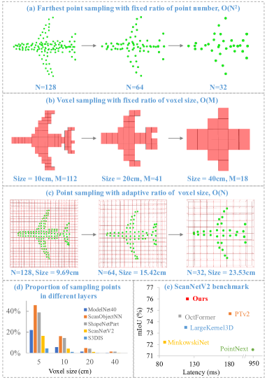
Figure 1: (a) Farthest point sampling with fixed ratio of point number, N means point number. (b) Voxel sampling with fixed ratio of voxel size, M means voxel number. (c) Point sampling with adaptive ratio of voxel size. (d) Proportion of sampled points in different layers. (e) Evaluation on ScanNetV2 validation set.

Point cloud learning is a crucial task for 3D scene understanding, such as autonomous driving and robotic systems [1, 2]. While the inputs often contain a large number of points in practical scenes, such that the downsampling process is critical for existing learning frameworks [3, 4, 5, 6]. Current samplers extract a representative subset from raw point clouds with point-, voxel- or learning-based designs [7, 8, 3, 4, 6]. However, there still remain great challenges to develop satisfying downsampling methods that ensure both efficiency and accuracy due to the commonly existing complex geometric structures and uneven distributions in real point data.

The most intuitive and efficient strategy is random sampling [9, 10]. But it easily neglects critical geometric and semantic information due to its random nature. To this end, Farthest Point Sampling (FPS) fully utilizes the distance prior for uniform sampling, thus achieving impressive accuracy and being the primary choice in most point-based networks [3, 11, 5]. In FPS, the number of sampled points is controllable [12], making it versatile for both indoor and outdoor scenes wherein the point clouds vary a lot for different scales and ranges. However, FPS is highly time-consuming, which requires computational complexity of $\mathcal{O}(N^{2})$ for distance measuring. That means FPS may occupy most of the time in the testing process, particularly for large-scale point clouds [4].

As an alternative, voxel-based methods have enjoyed significant success in large-scale 3D scene understanding due to their efficient designs. The original point cloud can be spatially divided into non-overlapping voxels by predefining the voxel size. Then, points within the same voxel are pooled into a single one before being fed into each network layer. Voxel sampling is quite efficient, which merely costs linear complexity, but it may leave another two problems: i) To predefine the voxel size across different 3D scenes is troublesome. As shown in Fig. 1(d), a fixed voxel size would produce significant differences in downsampling ratios. That means it causes over-sampling for point clouds. ii) Voxel-based sampling intrinsically loses fine-grained geometric structures. With the network going deeper, current methods require voxel sizes to be expanded by integer multiples (as commonly used $\times 2$), causing the voxel volume to increase by 8 times or more. Hence, the number of preserved points would be decreased dramatically after progressive downsamplings, as revealed in Fig. 1(d). This information loss often produces blurry/incorrect perceptions at object boundaries [13], which is the main reason for the low accuracy of existing voxel-based networks.

Additionally, researchers attempted to directly learn to downsample the raw point clouds by employing Multi-Layer Perceptrons (MLPs) [7, 14] or attention mechanisms [8]. However, this learning paradigm still operates on the entire 3D scenes, which involves extensive computation and memory budgets, limiting its applicability to large-scale point clouds. By contrast, the above-mentioned handcrafted designs [12, 3, 5, 15, 6] can adequately compress point clouds and are more practically used.

In this paper, we contribute to exploring an advanced sampler, namely Voxel Adaptation Module (VAM), that achieves both high efficiency and accuracy. In detail, we encourage the sampled results of our proposed VAM to mimic the good distribution of FPS. As shown in Fig. 1-(c), our VAM automatically adjusts the voxel size to adapt to the predefined downsampling ratio across the entire dataset. With such operation, the voxel size used in each layer can be scaled at an arbitrary ratio to adapt to different density distributions, which is more favorable for preserving fine-grained features compared to a fixed scaling factor. As FPS has been widely used in various point cloud tasks, the downsampling ratio based on FPS has undergone thorough ablation studies [12, 3, 11, 5]. Therefore, we can refer to the downsampling ratio used in point-based methods for configuration in practical applications.

Considering that existing learning frameworks [15, 16, 17] can not directly support the feature extraction from the arbitrary-ratio voxel size, we propose the AVS-Net network. A point dynamic grouping strategy is introduced to achieve point sampling and local structure aggregation with arbitrary voxel sizes. We validate the superiority of our approach on semantic segmentation and part segmentation tasks, which achieves state-of-the-art accuracy and promising efficiency.

Our contributions can be summarized as follows:

• We introduce the voxel adaptive module that automatically adjusts the voxel sizes for different scale scenes, referencing the point-based downsampling ratio.

• We propose the AVS-Net network with a dynamic point grouping strategy. It supports point sampling and feature extraction with arbitrary voxel sizes while maintaining high efficiency.

II Related Work

II-A Deep Learning on 3D Point Clouds

Point-based Methods commonly encode and learn directly from points without voxelization or projection to 2D images. The representative method, PointNet++ [12], adopts a hierarchical grouping structure for point sets and gradually extracts features of larger local areas along the hierarchy. Based on the PointNet++ [12] architecture, PointMLP [18] and PointNext [11] have made improvements in the network structure and training strategy, respectively, effectively improving the accuracy of point cloud analysis tasks. PCT[19], PTv1[3], PTv2[20], and other methods introduce self-attention into point-based methods, making them capable of remote information modeling and achieving excellent accuracy. However, expensive ball query or KNN algorithms make their efficiency a bottleneck.

Voxel-based Methods convert continuous point cloud data into discrete voxel representations, enabling the application of 3D convolutional neural networks to extract features. Representative methods include SparseConvNet[21], MinkowskiNet[15]. LargeKernel3D [6] applies large convolution kernels to 3D point cloud learning and proves beneficial in improving performance. OctFormer [22] proposes octree attention, which realizes efficient point cloud division and feature extraction. Voxel-based methods have good computational efficiency, but voxelization loses geometric details, which is not conducive to learning fine-grained features [23, 24].

II-B Voxel Sampling Methods

Voxel sampling divides 3D space into non-overlapping uniform grids, making the points easy to search. There are two primary methods for pooling those points within the same voxel. The most direct strategy is to use the central location as represent, i.e., voxel center sampling [25, 13, 26, 24]. After voxelization, deep models use integer indices of voxels for downsampling and neighbor search, as shown in Fig. 1-(b). For multi-layer networks, voxel size can be only scaled in integer multiples, which is limited by the implementation of their networks [16, 15, 17, 6]. Thus, voxel center sampling usually causes large quantization errors.

Another strategy is voxel centroid sampling, which averages the coordinates of the points within the same voxel as sampling. This approach preserves the accuracy of point positions to some extent, thereby retaining fine-grained geometric information [4]. On this basis, PTv2 [20], HAVSampler [27] and FastPointTrans [4] use this sampling approach to ensure accuracy. However, PTv2 [20] and HAVSampler [27] still employs expensive KNN/BallQuery for aggregating neighboring points. While FastPointTrans [4] maintains continuous point cloud coordinates, its underlying implementation still relies on MinkowskiEngine [15], such that its downsampling is limited by the voxel size of integer multiples. For instance, it cannot perform hierarchical sampling using the voxel size $[9.69\rightarrow 15.42\rightarrow 23.53]$ in Fig. 1-(c).

In this paper, we develop an adaptive voxel sampling strategy to cater to various scales of 3D scenes, better preserving the fine-grained geometric relationships of point clouds. Additionally, to support arbitrary voxel size sampling and feature extraction, we propose a novel learning framework, AVS-Net, which achieves high performance in both accuracy and efficiency, as revealed in Fig. 1-(e).

III METHOD

III-A Overview

In our method, AVS-Net first utilizes VAM to determine the voxel size for each downsampling layer, and then proceeds with model training and evaluation. For the segmentation task, AVS-Net employs a U-Net architecture that consists of an encoder and a decoder. For the classification task, AVS-Net comprises an encoder and a classification head. In the encoder part, we design the Voxel Set Abstraction (VSA) as the basic module. The details are introduced in Sec. III-B and shown in Fig. 2. Sec. III-C describes the adaptive voxel sampling in detail. As for the decoder, trilinear interpolation [12] is used to map the features of the downsampled subsets back to their respective supersets.

III-B Voxel Set Abstraction

The VSA module consists of two steps: intra-voxel feature extraction (Intra-VFE) and inter-voxel feature extraction (Inter-VFE). Intra-VFE utilizes voxel centroid sampling to aggregate the features of multiple points within the same voxel onto the sampled point. Unlike other voxel-based approaches that retain only voxel indices, our approach preserves the precise coordinate information of sampled points. This is crucial for extracting fine-grained information in point cloud analysis [4, 13, 26]. Inter-VFE fuses features among sampled points, which can expand the receptive field of the sampled points.

Unified data representation: As both voxel-based sampling and grouping algorithms involve dynamic numbers of points, we propose using $group\_id$ to express point grouping information explicitly. We utilize a two-dimensional tensor matrix as the data structure for point clouds and their features. Since model training involves the simultaneous processing of multiple-frames point clouds, we define each point $P_{i}$ with the following form:

$$P_{i}=[b,x,y,z,\textit{vc\_1d},group\_id].$$ (1)

Among these, $b$ represents the batch index, used to differentiate which frame’s point cloud each point belongs to. The number of points in different frames of point clouds can be unequal. The $xyz$ represents the point’s 3D spatial coordinates. The vc_1d is short for voxel_coord_1d, representing the one-dimensional voxel coordinates obtained by merging 3D voxel coordinates. The $group\_id$ signifies the point’s grouping information. In Intra-VFE, the $intra\_group\_id$ represents grouping information for multiple points belonging to the same voxel. In Inter-VFE, the $inter\_group\_id$ represents grouping information for the voxel-sampled point and its neighboring points.

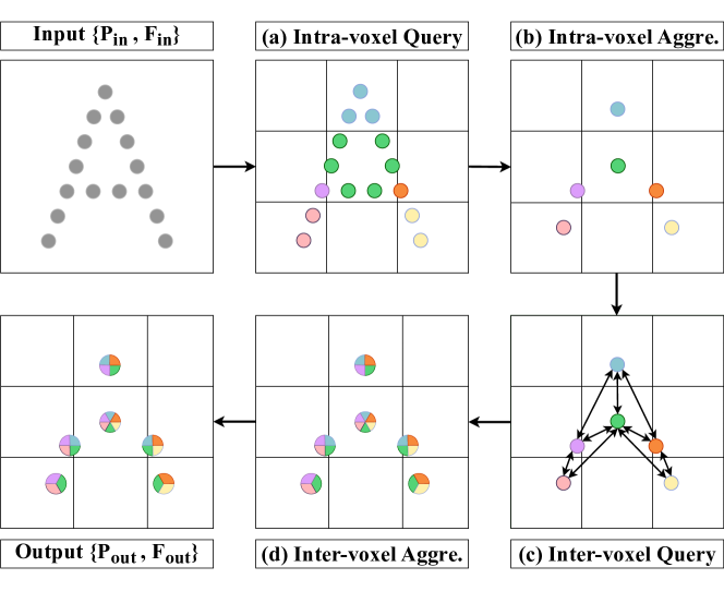
Figure 2: Schematic diagram of the Voxel Set Abstraction module

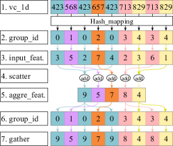
Figure 3: Scatter and gather operations.

Intra-voxel Query: Its flow is shown in Alg. 1. For input point set $P_{in}$, we first calculate the 3D voxel coordinates for each point and then flatten the 3D coordinates vc_3d into 1D coordinates vc_1d. The $\lfloor\cdot\rfloor$ is the floor function. If two points have the same vc_1d, it indicates that they are in the same voxel. Using vc_1d as the key, we obtain the $intra\_gid$ for each point through hash mapping. The $intra\_gid$ is short for $intra\_group\_{id}$. If there are $M$ non-empty voxels in the current batch, then $intra\_gid\in\{0,1,2,\ldots,M-1\}$. As shown in Fig. 2-(a), points with the same color within the same voxel are assigned to the same $intra\_gid$. The larger the vc_1d, the larger the corresponding $intra\_gid$, as illustrated in the first two rows of Fig. 3. Assuming the values of vc_1d are $\{423,568,657,713,829\}$, their corresponding $intra\_gid$ values are $\{0,1,2,3,4\}$. As the $voxel\_size$ in Alg. 1 can take any value, it allows for downsampling with arbitrary sizes in multi-layer networks.

Intra-voxel Aggregation: Since the number of points in each voxel is usually unequal, $scatter$ operations are employed during feature aggregation. $Scatter$ is a CUDA kernel library capable of various parallel computations on matrices based on $group-index$, including summation, maximum, average, and softmax operations, as shown in rows $2$-$5$ of Fig. 3. $Gather$ is the inverse operation of $scatter$, and by indexing and slicing the aggregated data. It aligns the aggregated data with the original input shape, as shown in rows $5$-$7$ of Fig. 3. For multiple points within the same voxel, we aggregate their coordinates and features onto a single sampled point. We take the average of the coordinates of multiple points for downsampling:

$$P_{s}=Mean_{scatter}(P_{in},intra\_gid).$$ (2)

Where $P_{s}$ represents the downsampled point cloud. After downsampling, there is only one sampled point within each voxel. For feature aggregation within voxels, local structural information is highly significant. We compute the local offset $\Delta P_{is}$ between multiple points within the voxel and the sampled point, concatenate this with $F_{in}$ (features of input points), and then apply MLP and max-pooling to obtain the aggregated features $F_{s}$.

$$\Delta P_{is}=P_{in}-Gather(P_{s},intra\_gid),$$ (3)

$$F_{s}=Max_{scatter}(MLP(F_{in}\oplus\Delta P_{is}),intra\_gid).$$ (4)

In Eq. 3, the $Gather$ operation aligns $M$ sampled points with the $N$ input points, as shown in rows $5$-$7$ of Fig. 3. In Fig. 2-(b), each voxel contains only one sampled point, which aggregates the features of all points within the voxel.

Input : Input Point Cloud $P_{in}[b,x,y,z]$

Output : 

intra_gid

Initialization

$voxel\_size$: voxel size used for sampling

$max\_r[x,y,z],min\_r[x,y,z]$: the upper and lower bound range of point cloud

$N[x,y,z]$ : the number of voxels on x,y,z axis

Procedure   $\textbf{Get\_3d\_Voxel\_Coords}(\mathbf{Points},voxel\_size)$

       $\mathbf{V[b]}=\mathbf{Points[b]}$;

       $\mathbf{V[x,y,z]}=\lfloor(\mathbf{Points[x,y,z]}-min\_r[x,y,z])/voxel\_size\rfloor$;

Return $\mathbf{V[b,x,y,z]}$

Procedure   $\textbf{Flatten\_3d\_to\_1d}(\mathbf{V},voxel\_size)$

       $N[x,y,z]=(max\_r[x,y,z]-min\_r[x,y,z])/voxel\_size$;

       $\mathbf{coord\_1d}=\mathbf{V[b]}\cdot N[x]\cdot N[y]\cdot N[z]+\mathbf{V[x]}\cdot N[y]\cdot N[z]+\mathbf{V[y]}\cdot N[z]+\mathbf{V[z]}$;

Return $\mathbf{coord\_1d}$

$\text{{vc\_3d}}={Get\_3d\_Voxel\_Coords}(\text{{$P_{in}$}},voxel\_size)$;

$\text{{vc\_1d}}={Flatten\_3d\_to\_1d}({\text{{vc\_3d}}},voxel\_size)$;

$\text{{intra\_gid}}={hash\_func}(\text{{vc\_1d}})$;

return intra_gid

Algorithm 1 Intra-voxel Query

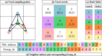
Figure 4: 2D example of Inter-voxel Query. (a) The spatial distribution of sampled points. (b) (0,0)-(2,2) represents the 2D coordinates of voxels, 0-8 are flattened vc_1d values, and 0,2,7 are empty voxels. (c) Hash table between vc_1d and voxel_index. (d) Neighbor indices and corresponding $group\_id$.

Inter-voxel Query: The Intra-VFE step allows feature aggregation for point clouds at arbitrary voxel sizes. To further expand the receptive field, we perform feature extraction for neighboring points of the sampled points. Since the aggregated sampled points have a one-to-one correspondence with voxels, we can efficiently perform the neighbor search using the Inter-voxel Query. The process of the Inter-voxel Query is outlined in Alg. 2, and a schematic diagram is given in Fig. 4.

The algorithm consists of three steps:

1) Given voxel-sampled point $P_{s}$, we first calculate its corresponding vc_1d, then obtain the voxel indices ($V_{indices}$) in memory with a hash mapping. We use vc_1d as the key and $V_{indices}$ as the value to construct a hash table $T_{hash}$.

2) Generate the local offset $O_{nbr}$ for 3D voxels based on the $nbr\_size$. For voxel coordinate $vc\_{3d}$, add the local offset $O_{nbr}$ to it, resulting in $[M,nbr\_size^{3},3]$ neighborhood coordinate matrix ${nbr\_3d}$ using broadcasting. Construct $[0,1,2,\ldots,M-1]^{T}$ with each element repeated $nbr\_size^{3}$ times as $inter\_gid$.

3) Within the $nbr\_size^{3}$ neighborhood of each non-empty voxel, there may be some empty voxels. We remove the empty voxels with hash lookup. For the remaining non-empty voxel set $nbr\_ne$, we use coord values as keys to find their corresponding $nbr\_{indices}$ in the $T_{hash}$. Finally, return $[nbr\_{indices},inter\_gid]$.

Inter-voxel Aggregation: Utilizing $nbr\_{indices}$, we can extract neighborhood feature matrices from non-empty voxel features $F_{s}$, as shown in Eq. 5. The relative position encoding of each point and its neighbor points is obtained by Eq. 8. We can use various operators to extract neighborhood features. As shown in Eq. 9, $f$ represents the neighborhood feature extraction operator, which can be an MLP, multi-head attention [28], or vector attention [20], etc. This paper uses vector attention [20] by default.

$$F_{nbr}=Gather(F_{s},nbr\_{indices}),$$ (5)

$$P_{nbr}=Gather(P_{s},nbr\_{indices}),\\$$ (6)

$$P_{center}=Gather(P_{s},inter\_gid),\\$$ (7)

$$\Delta P_{inter}=P_{nbr}-P_{center},\\$$ (8)

$$F_{out}=Sum_{scatter}(f(F_{nbr},\Delta P_{inter}),inter\_gid).$$ (9)

Complexity comparison. We denote $N$ as the number of input points, $M$ as the number of sampled points, and $K$ as the number of neighbors to search. Both $M$ and $N$ are much larger than $K$ in a large-scale point cloud. In previous point-based methods [12, 3, 11, 5], the complexities of FPS and KNN are $\mathcal{O}(MN)$ and $\mathcal{O}(MNlogK)$, respectively. In our method, the complexities of Intra-voxel Query and Inter-voxel Query are $\mathcal{O}(N)$ and $\mathcal{O}(MK)$. In this paper, $K=nbr\_size^{3}$, where $nbr\_size$ is typically equal to $3$. Our approach shares similar complexity with other voxel-based methods [21, 15, 17]. The key distinction is that our method retains precise coordinates of sampled points and allows for sampling and neighbor search at arbitrary voxel sizes at each layer.

Input : Voxel sampled points $P_{s}[B,x,y,z]$

Output : nbr_indices, inter_gid

Initilization

$voxel\_size$: voxel size used for partitioning

$\hskip 8.5359ptnbr\_size$: the number of neighbor points in each axis

Procedure   $\textbf{Generate\_Local\_Offset}(nbr\_size)$

       Local_Offset$\leftarrow[\hskip 2.84544pt];$

       $c=\lfloor nbr\_size/2\rfloor$;

       for $x$ $\mathbf{in}$ $range(nbr\_size)$ do

             for $y$ $\mathbf{in}$ $range(nbr\_size)$ do

                   for $z$ $\mathbf{in}$ $range(nbr\_size)$ do

                         Local_Offset$.append([x-c,y-c,z-c])$;

                   end for

                  

             end for

            

       end for

      

Return Local_Offset

$\text{{vc\_3d}}={Get\_3d\_Voxel\_Coords}(\text{{$P_{s}$}},voxel\_size)$;

$\text{{vc\_1d}}={Flatten\_3d\_to\_1d}(\text{{vc\_3d}},voxel\_size)$;

$\text{{V}}_{\text{{indices}}}={hash\_func}(\text{{vc\_1d}})$;

$\text{{T}}_{\text{{hash}}}=[\text{{vc\_1d}},\text{{V}}_{\text{{indices}}}]$;

${O_{nbr}}=\textit{Generate\_Local\_Offset}(nbr\_size)$;

$\text{{nbr\_3d}}=\text{{vc\_3d[x,y,z]}}+{O_{nbr}};$

$\text{{inter\_gid}}=[0,1,2,\ldots,len(\text{{vc\_3d}})-1]$;

$\text{{inter\_gid}}=\text{{inter\_gid}}.repeat(1,nbr\_size^{3})$;

$\text{{nbr\_1d}}={Flatten\_3d\_to\_1d}(\text{{nbr\_3d}},voxel\_size)$;

$\text{{mask}}={Find\_non\_empty\_voxels}(\text{{nbr\_1d}},\text{{vc\_1d}})$;

$\text{{nbr\_ne}}=\text{{nbr\_1d}}[\text{{mask}}]$;

$\text{{inter\_gid}}=\text{{inter\_gid}}[\text{{mask}}]$;

$\text{{nbr\_indices}}={hash\_find}(\text{{nbr\_ne}},\text{{T}}_{\text{{hash}}})$;

return nbr_indices, inter_gid

Algorithm 2 Inter-voxel Query

III-C Voxel Adaptation Module

Voxel size has a significant impact on the performance of voxel-based methods. The most crucial parameter affecting performance is the number of voxel sampled points. FPS can precisely control the downsampling ratio by controlling the number of sampled points. However, when using voxel sampling, the number of sampled points is unknown and dynamic for each point cloud frame. We propose using a fixed downsampling ratio as a reference to automatically adjust the voxel size, ensuring that the average sampling ratio over the entire dataset approaches this reference ratio. The proposed Voxel Adaptation Module (VAM) is used as a preprocessing module. Before model training, we use VAM to determine the voxel size for each layer. The voxel size remains constant during the training process.

In 3D space, the total number of voxels $N_{voxels}$, including empty voxels, is given by:

$$N_{voxels}=\frac{V_{space}}{voxel\_size^{3}}.$$ (10)

where $V_{space}$ is the volume of the 3D space. Since the distribution of point clouds in space is non-uniform, there is no strict equality relationship in Eq. 10. Intuitively, for the point clouds of the entire dataset, it is generally true that the larger the voxel size, the fewer the total number of non-empty voxels. This relationship can be approximately expressed as:

$$N_{s}\propto\ \frac{N_{i}}{voxel\_size^{3}},$$ (11)

$$voxel\_size\propto\ \sqrt[3]{\frac{N_{i}}{N_{s}}}.$$ (12)

Where $N_{i}$ and $N_{s}$ represent the sum of the number of input points and the sum of the number of voxel sampled points across the entire dataset. To make the sampling voxel size variable, we introduce a variable factor $Scale$. Therefore, the varable voxel size can be formulated as $voxel\_size=V_{0}\cdot\text{e}^{{Scale}}$, where $V_{0}$ is a constant value of the initial voxel size.

Since the mapping of input points to sampled points is obtained through a scatter operation on point indices, there is no gradient flow between the number of points and $voxel\_size$, making it impossible to train directly via the network. Inspired by the Proportional-Integral (PI) algorithm in automatic control, we have designed an algorithm for automatic voxel size adjustment. The algorithm’s flow and schematic are shown in Alg. 3 and Fig. 5.

We next introduce the PI method in detail. Alg. 3-i: For voxel sampling, given a downsampling ratio Ref_Ratio, we calculate the deviation $err$ by subtracting the actual sampling ratio corresponding to the current voxel size across the entire dataset from Ref_Ratio. Alg. 3-ii: Integrate $err$ to obtain the cumulative deviation $\sum{err}$, and add $err$ to $\sum{err}$. Alg. 3-iii: We adjust the scaling factor $Scale$ based on Diff. When Diff $>0$, it indicates that $N_{s}$ is too large, and the current voxel size is too small, so the $Scale$ increases. When Diff $<0$, the $Scale$ decreases. Alg. 3-iv: We calculate the actual voxel size that participates in the sampling based on $Scale$. Voxel_size is a monotonically increasing function with respect to $Scale$ and ensures non-negativity. The initial value of the $Scale$ is set to 0. We iterate over the entire dataset using Alg. 3-(i-iv). When $err$ is less than an extremely small value $\epsilon$, we consider it as reaching the convergence condition. At this point, $voxel\_size$ ensures that the average sampling ratio across the entire dataset approximates the given value Ref_Ratio. In Alg. 3, $V_{0}$, $I_{r}$, $K_{p}$, $K_{i}$, and $\epsilon$ are hyperparameters. $V_{0}$ is the initial voxel size, and $I_{r}$ is a parameter similar to the learning rate. $K_{p}$ and $K_{i}$ control the ratio of ${err}$ and $\sum{err}$, and $\epsilon$ controls the convergence condition. $\epsilon$ usually set to $0.1\%$.

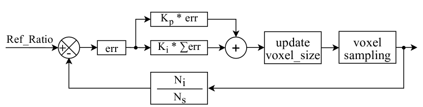
Figure 5: Voxel Adaptation Module via the PI control algorithm

while $err>\epsilon$ do

       $\text{i.}\ err=Ref\_Ratio-{N_{i}}\text{ / }{N_{s}}$;

      

       $\text{ii.}\ \textit{Diff}=K_{p}\cdot err+K_{i}\cdot\sum err$;

      

       $\text{iii.}\ Scale=Scale+I_{r}\cdot(\text{sigmoid}(\textit{Diff})-0.5)$;

      

       $\text{iv.}\ voxel\_size=V_{0}\cdot\text{e}^{Scale}$;

      

      

end while

Algorithm 3 VAM flow

IV Experiments

IV-A 3D Semantic Segmentation

ScanNetV2 [29] is a large-scale dataset widely used for analyzing 3D indoor scenes. We follow the setup of PTv2 [20] for training and evaluation. Tab. I presents the results of our method compared to previous methods on ScanNetV2 [29]. In Tab. II, we compare the number of parameters, latency, and mIoU with recent methods. We reproduce the results of each method on the validation set using their official code. To ensure a fair comparison, all methods pre-sample point clouds with $2cm$ voxel size, and mIoU do not involve TTA (without test-time augmentation). We use the same machine with an AMD EPYC 7313 CPU and a single NVIDIA 4090 GPU to measure the latency of methods. In Tab. II, latency is the average time taken for inference on each frame’s point cloud in the validation set. The batch size is set to 1.

In terms of accuracy, our AVS-Net achieves the best mIoU, as shown in Tab. II. In terms of efficiency, PointNeXt [11] has the highest latency due to the FPS downsampling method. PTv2 [20] employs efficient voxel sampling, which still incurs higher latency due to expensive KNN neighbor search. Our AVS-Net has similar latency to LargeKernel3D [6] but achieves gains of $2.5\%$ of mIoU. Our AVS-Net attains the highest mIoU on large-scale point clouds while maintaining high operational efficiency.

TABLE I: Semantic segmentation on ScanNetV2 val. set. TTA is test time augmentaion.

Method	Reference	Input	TTA	mIoU (%)
PointNet++ [12]	NeurIPS’17	point	✘	53.5
PointConv [30]	CVPR’19	point	✘	61.0
PointASNL [31]	CVPR’20	point	✘	63.5
JointPointBased [32]	3DV’19	point	✘	69.2
KPConv [33]	ICCV’19	point	✘	69.2
PTv1 [3]	ICCV’21	point	✔	70.6
PTv2  [20]	NeurIPS’22	point	✔	75.4
PointNeXt [11]	NeurIPS’22	point	✔	71.5
ADS  [34]	ICCV’23	point	✔	75.6
SparseConvNet [21]	CVPR’18	voxel	✘	69.3
MinkowskiNet [15]	CVPR’19	voxel	✘	72.2
FastPointTransformer [4]	CVPR’22	voxel	✘	72.1
Stratified Transformer [35]	CVPR’22	voxel	✔	74.3
LargeKernel3D  [6]	CVPR’23	voxel	✘	73.5
OctFormer  [22]	SIGGRAPH’23	voxel	✔	75.7
AVS-Net (ours)	-	voxel	✘	76.0

TABLE II: Latency and mIoU without TTA on ScanNetV2 val. set.

Method	Params. (M)	Latency (ms)	mIoU (%)
PointNeXt-XL [11]	41.6	951.5	71.5
MinkowskiNet-34 [15]	37.9	87.8	72.2
PTv2 [20]	11.3	181.4	74.7
LargeKernel3D [6]	40.2	118.2	73.5
OctFormer [22]	39.0	109.5	74.5
AVS-Net (ours)	20.9	120.4	76.0

IV-B Object Part Segmentation

ShapeNetPart [36] is an important dataset for fine-grained 3D shape segmentation. We follow the setup in PointNeXt [11] for training and evaluation. Regarding evaluation metrics, we report category mIoU and instance mIoU in Tab. III. Although the performance in ShapeNetPart is quite saturated, our AVS-Net achieves the highest category mIoU and instance mIoU with considerable improvements ($+0.3\%$ category mIoU). The integer multiples expansion of voxel size has resulted in an unreasonable sampling ratio, making it difficult for previous models with voxel sampling to achieve good results on small objects. However, our method surpasses all previous methods in Tab. III, demonstrating that our AVS-Net is also effective on small-scale(few number of points) datasets.

IV-C 3D Object Detection

We validate the effectiveness of AVS-Net in 3D object detection tasks. Specifically, we choose CenterPoint [37], a voxel-based method, as the baseline. And the 3D sparse convolutional networks [38] in CenterPoint is replaced with our AVS-Net, while the rest of the settings are kept unchanged. The detection accuracy for vehicles, pedestrians, and cyclists significantly improved after using our AVS-Net. The experimental results on the Waymo validation set are shown in Tab. IV. Compared to the prior best method DSVT-Voxel [2], our AVS-Net achieves comparable results, even slightly outperforming DSVT in the vehicles and pedestrians categories. This demonstrates the effectiveness of our AVS-Net.

IV-D VAM Convergence Experiment

We plot the curves of the down-sampling ratio with voxel size variation on the ShapeNetPart dataset. Different colors represent the four down-sampling layers of the network. As the voxel size increases, the average sampled points decrease, increasing the sampling rate. Fig. 6-(a) verifies that Eq. 12 is approximately valid.

On this basis, we adaptively adjust the voxel size using the PI control algorithm to match the given downsampling ratio, $Ref\_Ratio$. The scaling factor, $Scale$, is adjusted based on the actual sampling ratio. Fig. 6-(b) provides a specific example of how the scale changes. With a given downsampling ratio of $Ref\_Ratio=2$ and $\epsilon=0.1\%$, the initial voxel size, $V_{0}$, is set to $2.5cm$, and the initial $Scale$ is 0. Corresponding to this, the downsampling ratio is $1.14$. After $20$ epochs, the $Scale$ is adjusted to $0.708$, and according to Alg. 3-iv, the sampled voxel size becomes $5.07cm$. At this point, the downsampling ratio is $1.9999$, meeting the termination condition in Alg. 3. This experiment verifies that the PI control algorithm can make the downsampling ratio converge.

TABLE III: Part segmentation results on the ShapeNetPart.

Method	ins. mIoU	cat. mIoU
PointNet++ [12]	85.1	81.9
DGCNN [39]	85.2	82.3
KPConv [33]	86.4	85.1
CurveNet [40]	86.8	-
ASSANet-L [41]	86.1	-
PointMLP [18]	86.1	84.6
Stratifiedformer [35]	86.6	85.1
PTv1 [3]	86.6	83.7
PointNeXt  [11]	87.0	85.2
Point-PN  [5]	86.6	-
APES  [8]	85.8	83.7
ADS  [34]	86.9	-
SPoTr  [42]	87.2	85.4
AVS-Net (ours)	87.3	85.7

TABLE IV: Quantitative detection performance achieved by different methods on the Waymo [1] validation set (100% training data, single-frame setting). The best results are shown in bold.

Method	Reference	Vehicle (L1)		Vehicle (L2)		Pedestrian (L1)		Pedestrian (L2)		Cyclist (L1)		Cyclist (L2)
		mAP	mAPH	mAP	mAPH	mAP	mAPH	mAP	mAPH	mAP	mAPH	mAP	mAPH
SECOND [38]	Sensors’18	72.3	71.7	63.9	63.3	68.7	58.2	60.7	51.3	60.6	59.3	58.3	57.0
PointPillars [43]	CVPR’19	72.1	71.5	63.6	63.1	70.6	56.7	62.8	50.3	64.4	62.3	61.9	59.9
CenterPoint-Voxel [37]	CVPR’21	74.2	73.6	66.2	65.7	76.6	70.5	68.8	63.2	72.3	71.1	69.7	68.5
Part-$A^{2}$ [44]	TPAMI’20	77.1	76.5	68.5	68.0	75.2	66.9	66.2	58.6	68.6	67.4	66.1	64.9
PV-RCNN [26]	CVPR’20	78.0	77.5	69.4	69.0	79.2	73.0	70.4	64.7	71.5	70.3	69.0	67.8
PV-RCNN++ [45]	IJCV’22	79.3	78.8	70.6	70.2	81.3	76.3	73.2	68.0	73.7	72.7	71.2	70.2
SST [46]	CVPR’22	74.2	73.8	65.5	65.1	78.7	69.6	70.0	61.7	70.7	69.6	68.0	66.9
VoxSet [47]	CVPR’22	74.5	74.0	66.0	65.6	80.0	72.4	72.5	65.4	71.6	70.3	69.0	67.7
PillarNet-34 [48]	ECCV’22	79.1	78.6	70.9	70.5	80.6	74.0	72.3	66.2	72.3	71.2	69.7	68.7
CenterFormer [49]	ECCV’22	75.0	74.4	69.9	69.4	78.6	73.0	73.6	68.3	72.3	71.3	69.8	68.8
FlatFormer [50]	CVPR’23	77.5	77.1	69.0	68.6	79.6	73.0	71.5	65.3	71.3	70.1	68.6	67.5
DSVT-Voxel [2]	CVPR’23	79.7	79.3	71.4	71.0	83.7	78.9	76.1	71.5	77.5	76.5	74.6	73.7
AVS-Net (ours)	-	79.9	79.4	71.6	71.1	84.0	79.3	76.4	72.0	76.5	75.5	73.7	72.7

IV-E Ablation Study

TABLE V: Ablation on each component, evaluation on the ScanNetV2 val. set.

ID	Method	mIoU (%)	Latency (ms)
(1)	MinkowskiNet-34	72.2	87.8
(2)	(1)+Intra-VFE	73.5	75.5
(3)	(2)+VAM	75.7	74.9
(4)	Intra-VFE	72.4	71.8
(5)	(4)+Inter-VFE	74.9	131.8
(6)	(5)+VAM	76.0	120.4

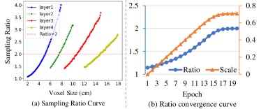
Figure 6: (a) The curve of the down-sampling ratio of the four-layer network as the voxel size changes. (b) Ratio convergence curve. The orange line represents the $Scale$ and the blue line represents the actual sampling ratio.

TABLE VI: $voxel\_size$ w.r.t. different $Ref\_Ratio$ settings for $4$-layer network on ShapeNetPart.

Ref_Ratio	Voxel size (cm)	ins. mIoU	cat. mIoU
1.5	[3.89, 5.25, 6.57, 8.02]	87.2	85.5
2	[5.07, 7.54, 10.58, 14.58]	87.3	85.7
3	[6.70, 11.62, 19.45, 35.14]	87.0	84.9
4	[7.89, 15.40, 31.22, 65.58]	86.9	84.7

TABLE VII: Latency (ms) of Sampling method and neighbor search algorithm.

Method	Number of points
	10k	20k	40k	80k	160k	320k
FPS	7.59	23.71	82.49	315.11	1217.06	4805.92
Intra-voxel Query	0.60	0.62	0.64	0.70	0.71	1.43
KNN	2.16	8.24	32.63	130.06	519.03	2082.33
Inter-voxel Query	1.41	1.42	1.69	2.76	6.08	12.06

The Effectiveness of Each Component. We conduct an ablation study using MinkowskiNet [15] and AVS-Net. MinkowskiNet voxelizes the point cloud and downsamples the voxels using “stride $=2$” convolutional layers, but it does not support downsampling with the arbitrary ratio of voxel size. We replace these convolutional layers with our intra-VFE, and replace the upsampling deconvolution layers with trilinear interpolation as the baseline, keeping the remaining parts unchanged. The experimental results are shown in Tab. V. Due to the preservation of precise geometric information in the point cloud by Intra-VFE, the performance is $1.3\%$ higher than the baseline without the quantization loss introduced by voxelization. In Tab. V-(2), the initial voxel size of the first layer is set to $2$cm, and four downsampling layers increase the voxel size by a factor of $2$ at each layer. In (3), we use a downsampling rate of $4$ to adaptively adjust the voxel size for each layer, resulting in gains of $2.2\%$ of mIoU.

In Tab. V-(4), we conducted ablation experiments using only the multi-layer Intra-VFE as the feature extraction module, treating it as a baseline. Tab. V-(5) and (6), we introduced Inter-VFE and VAM, respectively, resulting in a significant improvement in accuracy. The two sets of experiments in Tab. V validate the effectiveness of each proposed component in MinkowskiNet [15] and AVS-Net.

Ablation on Ref_Ratio in VAM. For downsampling methods, the downsampling ratio is a crucial parameter. The downsampling ratio based on FPS has undergone thorough ablation studies in point-based methods [12, 3, 11, 5]. Therefore, the used downsampling ratio in point-based methods is of great reference value for our VAM.

Tab. VI illustrates the correspondence between $Ref\_Ratio$ and $voxel\_size$ on the ShapeNetPart dataset. Different $Ref\_Ratio$s are used for the four downsampling layers, resulting in various $voxel\_size$ determined by the VAM. Specific numerical values indicate that the ratio between $voxel\_size$ in subsequent layers is arbitrary. On the ShapeNetPart dataset, the best results are obtained with a $Ref\_Ratio$ of 2. The optimal $Ref\_Ratio$ aligns with the downsampling ratio commonly used in previous point-based methods [12, 3, 11, 5].

Comparison on Latency of Different Sampling and Neighbor Search Methods. We compare the latency of different sampling methods and neighbor search methods. In Tab. VII, both FPS and Intra-voxel Query are set with a downsampling ratio of $4$. KNN and Inter-voxel Query perform neighbor point searches on the downsampled point clouds. For the latency test of each algorithm, we averaged $100$ runs. The time consumption of FPS and KNN increases quadratically with the number of points. In contrast, our proposed Intra-voxel and Inter-voxel Query algorithm show less noticeable changes when the point count is low due to the fixed time overhead of the $scatter$ operator. However, when the point count reaches $80k$, the time exhibits an apparent linear increase. For large-scale point clouds with number $\geq 320k$, our sampling method is $1000\times$ faster than FPS, and our neighbor search algorithm is $100\times$ faster than KNN.

V Conclusion

In this paper, we introduce the Voxel Adaption Module, which automatically adjusts voxel size based on the downsampling ratio to achieve a favorable balance between efficiency and accuracy. We also construct the AVS-Net that highly preserves geometric cues during sampling with efficient implementation of neighborhood search and feature aggregation. The proposed network can well support our adaptive voxel size design. Extensive experiments on multiple point cloud datasets have been conducted to demonstrate the superior accuracy and promising efficiency of our method.

References

- [1] P. Sun, H. Kretzschmar, X. Dotiwalla, A. Chouard, V. Patnaik, P. Tsui, J. Guo, Y. Zhou, Y. Chai, B. Caine, et al., “Scalability in perception for autonomous driving: Waymo open dataset,” in CVPR, 2020, pp. 2446–2454.
- [2] H. Wang, C. Shi, S. Shi, M. Lei, S. Wang, D. He, B. Schiele, and L. Wang, “Dsvt: Dynamic sparse voxel transformer with rotated sets,” in CVPR, 2023.
- [3] H. Zhao, L. Jiang, J. Jia, P. H. Torr, and V. Koltun, “Point transformer,” in ICCV, 2021, pp. 16 259–16 268.
- [4] C. Park, Y. Jeong, M. Cho, and J. Park, “Fast point transformer,” in CVPR, 2022, pp. 16 949–16 958.
- [5] R. Zhang, L. Wang, Y. Wang, P. Gao, H. Li, and J. Shi, “Starting from non-parametric networks for 3d point cloud analysis,” in CVPR, 2023, pp. 5344–5353.
- [6] Y. Chen, J. Liu, X. Zhang, X. Qi, and J. Jia, “Largekernel3d: Scaling up kernels in 3d sparse cnns,” in CVPR, 2023, pp. 13 488–13 498.
- [7] O. Dovrat, I. Lang, and S. Avidan, “Learning to sample,” in CVPR, 2019, pp. 2760–2769.
- [8] C. Wu, J. Zheng, J. Pfrommer, and J. Beyerer, “Attention-based point cloud edge sampling,” in CVPR, 2023, pp. 5333–5343.
- [9] H. Qi, C. Feng, Z. Cao, F. Zhao, and Y. Xiao, “P2b: Point-to-box network for 3d object tracking in point clouds,” in CVPR, 2020, pp. 6329–6338.
- [10] Q. Hu, B. Yang, L. Xie, S. Rosa, Y. Guo, Z. Wang, N. Trigoni, and A. Markham, “Randla-net: Efficient semantic segmentation of large-scale point clouds,” in CVPR, 2020.
- [11] G. Qian, Y. Li, H. Peng, J. Mai, H. Hammoud, M. Elhoseiny, and B. Ghanem, “Pointnext: Revisiting pointnet++ with improved training and scaling strategies,” NeurIPS, vol. 35, pp. 23 192–23 204, 2022.
- [12] C. R. Qi, L. Yi, H. Su, and L. J. Guibas, “Pointnet++: Deep hierarchical feature learning on point sets in a metric space,” NeurIPS, vol. 30, 2017.
- [13] F. Zhang, J. Fang, B. Wah, and P. Torr, “Deep fusionnet for point cloud semantic segmentation,” in ECCV. Springer, 2020, pp. 644–663.
- [14] I. Lang, A. Manor, and S. Avidan, “Samplenet: Differentiable point cloud sampling,” in CVPR, 2020, pp. 7578–7588.
- [15] C. Choy, J. Gwak, and S. Savarese, “4d spatio-temporal convnets: Minkowski convolutional neural networks,” in CVPR, 2019, pp. 3075–3084.
- [16] S. Contributors, “Spconv: Spatially sparse convolution library,” https://github.com/traveller59/spconv, 2022.
- [17] C. He, R. Li, S. Li, and L. Zhang, “Voxel set transformer: A set-to-set approach to 3d object detection from point clouds,” in CVPR, 2022, pp. 8417–8427.
- [18] X. Ma, C. Qin, H. You, H. Ran, and Y. Fu, “Rethinking network design and local geometry in point cloud: A simple residual MLP framework,” in ICLR, 2022. [Online]. Available: https://openreview.net/forum?id=3Pbra-˙u76D
- [19] M.-H. Guo, J.-X. Cai, Z.-N. Liu, T.-J. Mu, R. R. Martin, and S.-M. Hu, “Pct: Point cloud transformer,” Computational Visual Media, vol. 7, no. 2, pp. 187–199, 2021.
- [20] X. Wu, Y. Lao, L. Jiang, X. Liu, and H. Zhao, “Point transformer v2: Grouped vector attention and partition-based pooling,” NeurIPS, vol. 35, pp. 33 330–33 342, 2022.
- [21] B. Graham, M. Engelcke, and L. Van Der Maaten, “3d semantic segmentation with submanifold sparse convolutional networks,” in CVPR, 2018, pp. 9224–9232.
- [22] P.-S. Wang, “Octformer: Octree-based transformers for 3D point clouds,” ACM Transactions on Graphics (SIGGRAPH), vol. 42, no. 4, 2023.
- [23] H. Tang, Z. Liu, S. Zhao, Y. Lin, J. Lin, H. Wang, and S. Han, “Searching efficient 3d architectures with sparse point-voxel convolution,” in ECCV. Springer, 2020, pp. 685–702.
- [24] C. Zhang, H. Wan, X. Shen, and Z. Wu, “Pvt: Point-voxel transformer for point cloud learning,” International Journal of Intelligent Systems, vol. 37, no. 12, pp. 11 985–12 008, 2022.
- [25] Z. Liu, H. Tang, Y. Lin, and S. Han, “Point-voxel cnn for efficient 3d deep learning,” in NeurIPS, 2019.
- [26] S. Shi, C. Guo, L. Jiang, Z. Wang, J. Shi, X. Wang, and H. Li, “Pv-rcnn: Point-voxel feature set abstraction for 3d object detection,” in CVPR, 2020, pp. 10 529–10 538.
- [27] J. Ouyang, X. Liu, and H. Chen, “Hierarchical adaptive voxel-guided sampling for real-time applications in large-scale point clouds,” arXiv preprint arXiv:2305.14306, 2023.
- [28] A. Vaswani, N. Shazeer, N. Parmar, J. Uszkoreit, L. Jones, A. N. Gomez, Ł. Kaiser, and I. Polosukhin, “Attention is all you need,” NeurIPS, vol. 30, 2017.
- [29] A. Dai, A. X. Chang, M. Savva, M. Halber, T. Funkhouser, and M. Nießner, “ScanNet: Richly-annotated 3D reconstructions of indoor scenes,” in CVPR, 2017.
- [30] W. Wu, Z. Qi, and L. Fuxin, “Pointconv: Deep convolutional networks on 3d point clouds,” in CVPR, 2019.
- [31] X. Yan, C. Zheng, Z. Li, S. Wang, and S. Cui, “Pointasnl: Robust point clouds processing using nonlocal neural networks with adaptive sampling,” in CVPR, 2020.
- [32] H.-Y. Chiang, Y.-L. Lin, Y.-C. Liu, and W. H. Hsu, “A unified point-based framework for 3d segmentation,” in 3DV, 2019.
- [33] H. Thomas, C. R. Qi, J.-E. Deschaud, B. Marcotegui, F. Goulette, and L. J. Guibas, “Kpconv: Flexible and deformable convolution for point clouds,” in ICCV, 2019.
- [34] C.-Y. Hong, Y.-Y. Chou, and T.-L. Liu, “Attention discriminant sampling for point clouds,” in ICCV, 2023, pp. 14 429–14 440.
- [35] X. Lai, J. Liu, L. Jiang, L. Wang, H. Zhao, S. Liu, X. Qi, and J. Jia, “Stratified transformer for 3d point cloud segmentation,” in CVPR, 2022.
- [36] L. Yi, V. G. Kim, D. Ceylan, I.-C. Shen, M. Yan, H. Su, C. Lu, Q. Huang, A. Sheffer, and L. Guibas, “A scalable active framework for region annotation in 3d shape collections,” ACM TOG, 2016.
- [37] T. Yin, X. Zhou, and P. Krahenbuhl, “Center-based 3d object detection and tracking,” in CVPR, 2021, pp. 11 784–11 793.
- [38] Y. Yan, Y. Mao, and B. Li, “Second: Sparsely embedded convolutional detection,” Sensors, vol. 18, no. 10, p. 3337, 2018.
- [39] Y. Wang, Y. Sun, Z. Liu, S. E. Sarma, M. M. Bronstein, and J. M. Solomon, “Dynamic graph cnn for learning on point clouds,” ACM TOG, 2019.
- [40] T. Xiang, C. Zhang, Y. Song, J. Yu, and W. Cai, “Walk in the cloud: Learning curves for point clouds shape analysis,” in ICCV, 2021, pp. 915–924.
- [41] G. Qian, H. Hammoud, G. Li, A. Thabet, and B. Ghanem, “Assanet: An anisotropic separable set abstraction for efficient point cloud representation learning,” NeurIPS, vol. 34, 2021.
- [42] J. Park, S. Lee, S. Kim, Y. Xiong, and H. J. Kim, “Self-positioning point-based transformer for point cloud understanding,” in CVPR, 2023, pp. 21 814–21 823.
- [43] A. H. Lang, S. Vora, H. Caesar, L. Zhou, J. Yang, and O. Beijbom, “Pointpillars: Fast encoders for object detection from point clouds,” in CVPR, 2019, pp. 12 697–12 705.
- [44] S. Shi, Z. Wang, J. Shi, X. Wang, and H. Li, “From points to parts: 3d object detection from point cloud with part-aware and part-aggregation network,” IEEE TPAMI, vol. 43, no. 8, pp. 2647–2664, 2020.
- [45] S. Shi, L. Jiang, J. Deng, Z. Wang, C. Guo, J. Shi, X. Wang, and H. Li, “Pv-rcnn++: Point-voxel feature set abstraction with local vector representation for 3d object detection,” IJCV, pp. 1–21, 2022.
- [46] L. Fan, Z. Pang, T. Zhang, Y.-X. Wang, H. Zhao, F. Wang, N. Wang, and Z. Zhang, “Embracing single stride 3d object detector with sparse transformer,” in CVPR, 2022.
- [47] C. He, R. Li, S. Li, and L. Zhang, “Voxel set transformer: A set-to-set approach to 3d object detection from point clouds,” in CVPR, 2022.
- [48] G. Shi, R. Li, and C. Ma, “Pillarnet: Real-time and high-performance pillar-based 3d object detection,” in ECCV, 2022.
- [49] Z. Zhou, X. Zhao, Y. Wang, P. Wang, and H. Foroosh, “Centerformer: Center-based transformer for 3d object detection,” in ECCV, 2022.
- [50] Z. Liu, X. Yang, H. Tang, S. Yang, and S. Han, “Flatformer: Flattened window attention for efficient point cloud transformer,” in CVPR, 2023, pp. 1200–1211.