The Strong CP Problem in the Quantum Rotor

Abstract

Recent studies have claimed that the strong CP problem does not occur in QCD, proposing a new order of limits in volume and topological sectors when studying observables on the lattice. In order to shed light on this issue, we study the effect of the topological $\theta$-term on a simple quantum mechanical rotor that allows a lattice description. The topological susceptibility and the $\theta$-dependence of the energy spectrum are both computed using local lattice correlation functions. The sign problem is overcome by considering Taylor expansions in $\theta$ exploiting automatic differentiation methods for Monte Carlo processes. Our findings confirm the conventional wisdom on the strong CP problem.

I Introduction

The strong CP problem remains as one of the puzzles of the Standard Model: why do the strong interactions conserve CP? In principle, the Lagrangian of Quantum Chromodynamics (QCD) admits a renormalizable gauge invariant $\theta$-term,

$$\delta\mathcal{L}_{\theta}=\frac{\theta}{16\pi^{2}}{\rm tr}\left(F_{\mu\nu}\tilde{F}^{\mu\nu}\right)\,,$$ (1)

where $F_{\mu\nu}=\partial_{\mu}A_{\nu}-\partial_{\nu}A_{\mu}+[A_{\mu},A_{\nu}]$ is the field strength and $A_{\mu}$ the gauge connection. While the presence of such a term would break CP symmetry in QCD, experimental measurements of the electric dipole moment of the neutron constrain the coupling to be $|\theta|\lesssim 10^{-10}$ [1].

Many solutions have been proposed over the years. The existence of a massless quark would make the $\theta$ phase unphysical, but recent lattice simulations clearly disfavor such a solution [2]. Additionally, various alternatives beyond the Standard Model, such as a Peccei-Quinn symmetry [3] and Nelson-Barr type models [4, 5], have been explored.

It has been claimed in refs. [6, 7] that the effect of a such a $\theta$-term, even if present, would not lead to observable consequences. These works argue that when computing correlation functions, the infinite volume limit should be taken before the summation over topological sectors. The consequence of such an order of limits (infinite volume at each fixed topological charge) would be the absence of $\theta$-dependence from observables, and particularly from the energy spectrum of the theory.

We claim that, in fact, the order of limits is only important if one insists in computing global observables, i.e. those computed as an integral over the whole Euclidean space. Determining these observables requires extreme care with the role of boundary conditions and in taking the infinite volume limit. On the other hand they also represent quite unphysical setups, since we do not need to know the boundary conditions of the universe to measure the topological susceptibility, the proton mass, or the neutron electric dipole moment: all physical quantities of interest can be extracted from local correlators. Due to clustering, the dependence of local correlators on the boundary conditions or the finite volume is exponentially suppressed in theories with a mass gap, making the order of limits largely irrelevant.

In this paper, we aim to shed some light on this question by examining a simple toy model that, nevertheless, shares some key characteristics with QCD: the quantum rotor. We will compute the topological susceptibility from local correlators and show that, up to finite volume corrections, the result is independent of the choice of boundary conditions. The analytical computations will also be supported by numerical lattice simulations, validating the approach used by the lattice community to answer these questions in QCD [8, 9, 10]. Additionally, we will determine the topological susceptibility using master field simulations [11], where a single gauge configuration in a very large Euclidean volume allows to determine expectation values as volume averages. Both local computations give the same non-zero value for the topological susceptibility, $\chi_{t}$. Moreover, we will show that the spectrum of the theory has a dependence on $\theta$.

Finally, the numerical study of this rather simple system faces several challenging problems present in lattice QCD. We will use several recent proposals to overcome these problems, making the study of this particular model a good test-bed for many state-of-the-art lattice techniques. Firstly, the issue of topology freezing [12, 13, 14, 15] when approaching the continuum limit is solved by the use of winding transformations [16]. Secondly, simulating the theory at a non-zero value of $\theta$ leads to the so-called sign problem —see [17, 18] and references therein. We employ three different methods to overcome this, which rely on the use of imaginary values for $\theta$ along with analytical continuation [19, 20, 21, 22, 23, 24, 25, 26, 27, 28, 29]: on the one hand, we will extract the $\theta$ dependence by a fit to data from several simulations at different imaginary values of $\theta$; on the other hand, we will explore two recent proposals that allow to extract series expansions in $\theta$ using automatic differentiation for Monte Carlo processes [30].

The paper is organized as follows: in section II we introduce the quantum rotor, along with the action and topological charge definitions in the continuum and on the lattice, including two different choices of discretization; in section III we study the order of limits argued in refs. [6, 7] and the conventional one using both global and local observables, where the latter are computed with lattice simulations; in section IV we obtain the continuum $\theta$-dependence of the energy spectrum from lattice simulations using different boundary conditions —this computation requires overcoming the sign problem, whose proposed solutions are introduced in section IV.1.

II The quantum rotor

The quantum rotor describes a free particle of mass $m$ on a ring of radius $R$. The system admits a $\theta$-term and can be formulated at finite temperature $\beta=1/T$ as a path integral with partition function [31, 32]

$$Z(\theta)=\int\mathcal{D}\phi\,e^{-S(\phi)+i\theta Q},$$ (2)

where the action reads

$$S(\phi)=\frac{I}{2}\int_{0}^{T}dt\,\dot{\phi}(t)^{2}\,,$$ (3)

with $\phi(0)=\phi(T)$ and $-\pi<\phi(t)\leq\pi$, and where we have defined the moment of inertia $I=mR^{2}$. Note that using periodic boundary conditions leads to the quantization of the topological charge,

$$Q=\frac{1}{2\pi}\int_{0}^{T}dt\,\dot{\phi}(t)\,\in\mathbb{Z}.$$ (4)

To study the system on a lattice we divide the time extent $T\equiv\hat{T}a$ into a lattice of $\hat{T}$ points with spacing $a$, and express the moment of inertia measured in units of this lattice spacing as $\hat{I}=I/a$. There are several possibilities for the discretization of the lattice action, with the only condition being that the continuum action and topological charge in eqs. (3) and (4) are recovered in the limit $\hat{I}\to\infty$ with

$$\frac{T}{I}=\frac{\hat{T}}{\hat{I}}=\text{constant}.$$ (5)

Particularly, we will use the so-called classical perfect action [33],

$$S_{\rm cp}(\phi)=\frac{\hat{I}}{2}\sum_{t=0}^{\hat{T}-1}((\phi_{t+1}-\phi_{t})\bmod 2\pi)^{2}\\ ,$$ (6)

as well as the standard action,

$$S_{\rm st}(\phi)=\frac{\hat{I}}{2}\sum_{t=0}^{\hat{T}-1}(1-\cos(\phi_{t+1}-\phi_{t}))\,.$$ (7)

One can show that the classical perfect action has smaller lattice artifacts and therefore a better behavior as one approaches the continuum limit [32]. However, the standard discretization is useful when using sampling algorithms that require the derivative of the action with respect to the field to be defined at all points of its domain. Particularly, we will use the Hybrid Monte Carlo (HMC) [34, 35] algorithm to overcome the sign problem when studying the $\theta$ dependence of the spectrum of the theory.

Analogously, we define the classical perfect topological charge,

$$Q_{\rm cp}=\frac{1}{2\pi}\sum_{t=0}^{\hat{T}-1}((\phi_{t+1}-\phi_{t})\bmod 2\pi),$$ (8)

and the standard topological charge,

$$Q_{\rm st}=\frac{1}{2\pi}\sum_{t=0}^{\hat{T}-1}\sin(\phi_{t+1}-\phi_{t}).$$ (9)

Note that with periodic boundary conditions the classical perfect topological charge is exactly an integer, while the standard one is only an integer in the continuum limit.

III On the order of limits of infinite volume and topological sectors

For theories with topology the computation of an observable can be decomposed as a sum of contributions from the different topological sectors,

$$\expectationvalue{\mathcal{O}}=\sum_{Q}\expectationvalue{\mathcal{O}}_{Q}p(Q),$$ (10)

where $p(Q)$ is the probability density of the topological sector with charge $Q$, and $\left<\dots\right>_{Q}$ denotes expectation value at fixed topological sector $Q$. While this equation is general, it requires the topological charge $Q$ to be quantized. For gauge quantum field theories, the usual reasoning for the quantization of the topological charge arises from the requirement of finite saddle solutions for the action, which constrains the gauge configurations at infinity to be pure gauge (i.e. a gauge transformation of zero).

In practice, lattice calculations are restricted to finite Euclidean volumes. This, together with the above reasoning, led the authors of refs. [6, 7] to challenge the conventional order of limits to extract observables at infinite volume. Namely, they propose to compute observable quantities as

$$\expectationvalue{\mathcal{O}}=\lim_{N\rightarrow\infty}\lim_{T\rightarrow\infty}\sum_{\absolutevalue{Q}<N}\expectationvalue{\mathcal{O}}_{Q}p(Q),$$ (11)

such that the volume is taken to infinity before the contributions from all the topological sectors are summed.

This claim can be verified in the quantum rotor, which can be trivially solved using the quantum mechanical formalism [32]. The energy levels of the system read

$$E_{n}=\frac{1}{2I}\left(n-\frac{\theta}{2\pi}\right)^{2},\quad n\in\mathbb{Z}\,.$$ (12)

In Euclidean time with periodic boundary conditions we have the thermal partition function

$$Z(\theta)=\sum_{n\in\mathbb{Z}}e^{-TE_{n}}=\sum_{n\in\mathbb{Z}}e^{-\frac{T}{2I}\left(n-\frac{\theta}{2\pi}\right)^{2}},$$ (13)

from which we can obtain the second moment of the topological charge at $\theta=0$,

$$\langle Q^{2}\rangle =-\frac{\partial\log Z(\theta)}{\partial\theta}\Big{|}_{\theta=0}$$

$$=\frac{T}{4I\pi^{2}}\left(1-\frac{\sum_{n}n^{2}e^{-\frac{T}{2I}n^{2}}}{\sum_{n}e^{-\frac{T}{2I}n^{2}}}\right)\,.$$ (14)

Note that for large $T$ we have

$$\frac{\langle Q^{2}\rangle}{T}=\frac{1}{4I\pi^{2}}\left[1-\frac{T}{I}\left(e^{-\frac{T}{2I}}-e^{-\frac{T}{I}}\right)+\dots\right],$$ (15)

i.e. a non-zero value with exponentially small corrections due to the finite size of the system. This leads to the usual result for the topological susceptibility,

$$\chi_{t}=\lim_{T\to\infty}\frac{\langle Q^{2}\rangle}{T}=\frac{1}{4I\pi^{2}}\,.$$ (16)

We can, instead, attempt to take the infinite $T$ limit before summing over topological sectors. To do this, we can determine the probability distribution of each topological sector of charge $Q$. Considering $\theta=0$ for simplicity we have

$$p(Q)= \frac{1}{2\pi Z(0)}\int_{-\pi}^{\pi}d\theta\,Z(\theta)e^{-i\theta Q}$$

$$= \frac{1}{Z(0)}\sqrt{\frac{2I\pi}{T}}\exp\left(-\frac{2I\pi^{2}}{T}Q^{2}\right).$$ (17)

According to [6] the correct order of limits should now read

$$\chi_{t} =\lim_{N\to\infty}\lim_{T\to\infty}\frac{1}{T}\sum_{\absolutevalue{Q}<N}Q^{2}\,p(Q)\,$$

$$=\lim_{N\to\infty}\lim_{T\to\infty}\frac{1}{T}\frac{\sum_{|Q|\leq N}Q^{2}\exp(-\frac{2\pi^{2}I}{T}Q^{2})}{\sum_{|Q|\leq N}\exp(-\frac{2\pi^{2}I}{T}Q^{2})},$$ (18)

which is trivially zero, and therefore contradicts the result in eq. 16.

To shed some light into this discrepancy, we propose another approach in which the order of limits is irrelevant. Due to locality, Euclidean two-point functions decay exponentially at large time separations, a fact that can be exploited to compute the topological susceptibility from local correlators. If one defines the topological charge density as $q(t)=\dot{\phi}(t)$ we have

$$\langle Q^{2}\rangle = \sum_{t_{1},t_{2}}\langle q(t_{1})q(t_{2})\rangle=T\sum_{t}\langle q(t)q(0)\rangle$$ (19)

$$= T\sum_{t<R}\langle q(t)q(0)\rangle+\mathcal{O}(e^{-R/\xi})\,,$$

where the last sum runs over a time extent $R$ and $\xi$ represents the correlation length of the system, which for the quantum rotor reads $\xi=(E_{1}-E_{0})^{-1}=2I$. Therefore one can compute the topological susceptibility in a localized region of radius $R\ll T$,

$$\chi_{t}=\sum_{t<R}\langle q(t)q(0)\rangle+\mathcal{O}(e^{-R/\xi}),$$ (20)

where contributions from $t>R$ are exponentially suppressed. The following observations follow:

1. Since $R\ll T$ and finite volume effects in eq. 20 are $\mathcal{O}(e^{-T/\xi})$, they are even more exponentially suppressed. As we will see, any choice of boundary conditions must give the same result.

2. In eq. 20 there is no sum over topological sectors and, in fact, $\displaystyle\frac{1}{2\pi}\sum_{t<R}q(t)$ is not quantized. There is no order of limits to discuss.

It is easy to compute observables in the quantum rotor using open boundary conditions. Concretely, the two-point correlation function of the topological density, which we derive in app. A, yields

$$\langle q(t_{1})q(t_{2})\rangle_{\text{cp, OBC}}=\delta_{t_{1},t_{2}}\left[\frac{1}{4I\pi^{2}}+\mathcal{O}(I^{-2})\right]\,.$$ (21)

In this particular case, finite time-extent effects are completely absent and one can just set $R=1$ in eq. 20. In the continuum limit we then have

$$\lim_{I\to\infty}I\chi_{t}=\frac{1}{4\pi^{2}},$$ (22)

which coindices with the result in eq. 16.

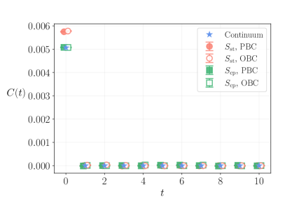
Figure 1: The quantity $C(t)\equiv\langle q(t)q(0)\rangle$ as a function of $t$ from simulations at $\hat{I}=5$ and $\hat{T}=100$ with the standard action (red circles) and classical perfect action (green squares) with open boundary conditions (open symbols) and periodic boundary conditions (filled symbols). The blue stars represent the continuum result.

One can use lattice simulations to obtain the same result using periodic boundary conditions instead. Although in this model topology freezing is already apparent at rather small values of the coupling $\hat{I}$, we overcome it by using a combination of standard Metropolis updates [37] and winding transformations [16] (see app. C).

In fig. 1 we show the topological two-point function as a function of $t$ for the standard action (red circles), and the classical perfect action (green squares), as well as for open (open symbols) and periodic (filled symbols) boundary conditions. The continuum result is also shown (blue stars). It is worth noting that the case with periodic boundary conditions should have a similar $t$-dependence as the correlator for open boundaries, $\langle q(t_{1})q(t_{2})\rangle\propto\delta_{t_{1},t_{2}}$, up to exponentially small finite-volume effects.

On the other hand, the discrepancy between the standard and classical perfect actions is a discretization effect that disappears taking the continuum limit. This can be seen in fig. 2, where we show the continuum extrapolation of $I\chi_{t}$ with simulations at constant $T/I=20$ for the classical perfect action (green, open circles) and for the standard action (red, filled circles) with periodic boundary conditions. The red and green dashed lines are the corresponding analytic curves with open boundary conditions, and one can see that both choices of discretization and boundary conditions give the same non-zero results for $\hat{I}\rightarrow\infty$.

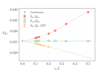
Figure 2: Continuum extrapolation of $\chi_{t}$ computed from $\langle q(t)^{2}\rangle$ at various $\{\hat{T},\hat{I}\}$ at constant $T/I=20$ with the standard action and classical topological charge (red, filled circles), with the classical action and topological charge (green, open circles) and from master field simulations with the standard action and topological charge (orange, open squares), all with periodic boundary conditions. The topological charges of the master fields, from smaller to larger value of $\hat{I}$, are $Q=-83,-61,-233,11,24,-118$. The dashed lines represent the corresponding analytical results with open boundary conditions.

Finally, the orange squares come from master field simulations using the standard action with periodic boundary conditions. Concretely, every point comes from the volume average of the local definition of the topological susceptibility in eq. 20 on a single master field configuration with $T=10^{6}$, and with the standard definition of the topological charge of eq. 9. Although these configurations can have very large values of the topological charge, the result, once extrapolated to the continuum, matches eq. 16.

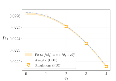
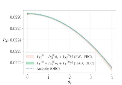
Figure 3: $\theta_{I}$ dependence of $I\chi_{t}$ at $\hat{I}=5$ and $\hat{T}=100$ with periodic boundary conditions and with different methods. Left frame: results (orange circles) from 5 different simulations with 100k uncorrelated configurations each, along with their fit to the functional form $f(\theta_{I})=a+b\theta_{I}+c\theta_{I}^{2}$. Right frame: results from single simulations with 500k uncorrelated configurations using reweighting and HAD (red and green points) at $\theta_{I}=0$, along with the curve $I\chi_{t}^{(0)}+I\chi_{t}^{(1)}\theta_{I}+I\chi_{t}^{(2)}\theta_{I}^{2}$ (light-red and thick-green bands) obtained from the use of truncated polynomials. The reweighting was performed on a simulation with periodic boundary condition, while HAD was used with open boundary conditions. In both frames the analytic result from open boundary conditions is displayed (dashed line).

IV On the $\theta$ dependence of the spectrum

The spectrum of the quantum rotor is changed by the presence of the $\theta$-term, as seen in eq. 12. However, and similarly to the previous section, we are interested in obtaining this dependence explicitly from local correlators on the lattice. The obvious challenge in this computation is the sign problem arising from the imaginary term in the partition function of eq. 2 when $\theta\neq 0$.

IV.1 Overcoming the sign problem on the lattice

A common approach around the sign problem is to perform simulations at an imaginary value of $\theta$ by defining $\theta_{I}=i\theta\in\mathbb{R}$. This makes the integrand in eq. 2 become real and allows to investigate the $\theta$-dependence of observables using standard sampling algorithms. Analyticity around $\theta=0$ of the observable $O$ under study is also a required assumption, i.e.

$$O(\theta)=O^{(0)}+O^{(1)}\theta+O^{(2)}\theta^{2}+\mathcal{O}(\theta^{3}),$$ (23)

with the expansion coefficients

$$O^{(n)}=\frac{1}{n!}\evaluated{\partialderivative[n]{O}{\theta}}_{\theta=0}.$$ (24)

From this we can obtain the expansion coefficient $O^{(n)}$ from analytic continuation and fits to data. Particularly, in fig. 3 (left) we show results of $I\chi_{t}$ at different $\theta_{I}$ at $\hat{I}=5$, along with a fit to the functional form $f(x)=a+bx+cx^{2}$ with parameters $a,b,c\in\mathbb{R}$.

This method has been used recently to study the $\theta$-dependence of the energy spectrum of four-dimensional SU($N$) Yang–Mills theories [29]. One of its drawbacks, however, is that it requires several simulations to extract the different expansion coefficients.

Alternatively, it is possible obtain arbitrarily high expansion coefficients by performing a single simulation where the Taylor expansion in $\theta$ is done automatically using the algebra of truncated polynomials [38]. From the point of view of the lattice implementation, the idea is to define a new field, $\tilde{\phi}$, as a power series expansion in $\theta$ up to some order $K$, i.e.

$$\tilde{\phi}(\theta)\equiv\tilde{\phi}^{(0)}+\tilde{\phi}^{(1)}\theta+\tilde{\phi}^{(2)}\theta^{2}+\dots+\tilde{\phi}^{(K)}\theta^{K}.$$ (25)

All basic operations and functions acting on these truncated polynomials are defined to be exact at each order, and therefore the computation of observables preserves the correct derivatives with respect to $\theta$. For more details about the implementation of automatic differentiation using truncated polynomials and applications to stochastic processes, see [30].

The simplest application of truncated polynomials to extract higher order derivatives is by using reweighting techniques. Starting from an already existent ensemble of configurations generated at $\theta=0$, reweighting allows the computation of expectation values for $\theta\neq 0$ by using the identity

$$\expectationvalue{O(\phi)}_{\theta}=\frac{\expectationvalue{e^{i\theta Q}O(\phi)}_{\theta=0}}{\expectationvalue{e^{i\theta Q}}_{\theta=0}},$$ (26)

where $\left<\cdots\right>_{\theta}$ denotes expectation value with respect to the probability distribution $p(\phi)=\frac{1}{Z(\theta)}e^{-S(\phi)+i\theta Q}$.

To extract the Taylor expansion of $\left<O(\phi)\right>_{\theta}$ with respect to $\theta$ up to order $K$ we replace $\theta$ with a truncated polynomial $\tilde{\theta}=\sum_{k=0}^{K}\tilde{\theta}^{(k)}\theta^{k}$ where $\tilde{\theta}^{(1)}=1$ and $\tilde{\theta}^{(k\neq 1)}=0$. The factor $\exp(i\theta Q)$ and also the numerator and denominator of eq. 26 thus become truncated polynomials. Therefore, by performing reweighting on a single ensemble we obtain the full analytical dependence of the polynomial expansion. This is shown in fig. 3 (right), where by reweighting a single standard simulation at $\theta_{I}=0$ with periodic boundary conditions we automatically obtain $I\chi_{t}^{(k)}$; particularly, we show $I\chi_{t}^{(0)}+I\chi_{t}^{(1)}\theta_{I}+I\chi_{t}^{(2)}\theta_{I}^{2}$ in the (light) red band, which agrees with the analytical result (dashed line) obtained with open boundary conditions.

An alternative application of truncated polynomials consists in a modification of sampling algorithms based on Hamiltonian dynamics inspired in Numerical Stochastic Perturbation theory [40, 41]. Particularly, we consider a modification of the HMC algorithm which we denote as Hamiltonian Automatic Differentiation (HAD), but this modification can be easily applied to other sampling methods. For the quantum rotor, since differentiability with respect to the field is required in the HMC equations of motion, it is necessary to use the standard discretization of the action and topological charge in eqs. (7) and (9). Concretely, with periodic boundary conditions the equations of motion read

$$\dot{\phi}_{t}= \frac{\partial H(\pi,\phi)}{\partial\pi_{t}}=\pi_{t},$$

$$\dot{\pi}_{t}= -\frac{\partial H(\pi,\phi)}{\partial\phi_{t}}$$ (27)

$$= -I\left[\sin(\phi_{t}-\phi_{t-1})-\sin(\phi_{t+1}-\phi_{t})\right]$$

$$+\theta_{I}\frac{1}{2\pi}\left[\cos(\phi_{t}-\phi_{t-1})-\cos(\phi_{t+1}-\phi_{t})\right],$$

where $t\in[0,\hat{T}-1]$, the dot denotes derivative with respect to Monte Carlo time, $\pi$ is the canonical conjugate momenta of $\phi$, and $H(\pi,\phi)=\sum_{t=0}^{\hat{T}-1}\pi_{t}^{2}/2+S_{\text{cp}}(\phi)-\theta_{I}Q_{\text{cp}}$ is the Hamiltonian of the system.

To extract deritatives with respect to $\theta_{I}$ we replace it by a truncated polynomial, $\tilde{\theta}_{I}$. This way, $\phi$ and $\pi$ become truncated polynomials as well, and section IV.1 becomes a set of differential equations where each order involves only terms of the same or lower order.

The use of truncated polynomials within the solver of the equations of motion automatizes the sampling. Therefore, after a single HMC simulation with truncated polynomials we obtain a Markov chain of $N$ samples, $\{\tilde{\phi}_{(i)}\}_{i=1}^{N}$, that carry the derivatives with respect to $\theta_{I}$. The Taylor expansion of observables is obtained by the computation of conventional expectation values using these samples.

Method	$\chi_{t}^{(0)}\times 10^{-3}$	$\chi_{t}^{(2)}\times 10^{-6}$
Fit	4.5238(16)	-6.08(48)
Reweighting	4.52501(76)	-5.99(25)
HAD	4.52604(83)	-5.980(34)

Table 1: Comparison of errors between different methods to obtain the $\theta_{I}$-dependence, namely, the quadratic fit to the results from direct simulations at $\theta_{I}$ (fig. 3 left), reweighting, and HAD (fig. 3 right). These results correspond to simulations with $\hat{I}=5$ and $\hat{T}=100$, using the standard definitions of the action and topological charge.

In fig. 3 (right) we show the curve $I\chi_{t}^{(0)}+I\chi_{t}^{(1)}\theta_{I}+I\chi_{t}^{(2)}\theta_{I}^{2}$ in (thick) green obtained from a single HAD simulation, and one can appreciate that the predictions for high $\theta_{I}$ are more accurate than the ones obtained by reweighting. This can be seen more transparently in tab. 1, where we show the results for $\chi_{I}^{(0)}$ and $\chi_{I}^{(2)}$ obtained with the three methods with an equivalent amount of statistics. Focusing on $\chi_{t}^{(2)}$ one can see that the reweighting result has an improved accuracy with respect to the value obtained by simulating directly at imaginary values of $\theta$; on the other hand, the error obtained with HAD is an order of magnitude smaller, although one should also consider the additional computational overhead coming from the operations of truncated polynomials.

IV.2 Spectrum from lattice correlators

To extract the energy spectrum on the lattice we use the spectral decomposition of an operator $O$,

$$C(t)=\expectationvalue{O(t)O(0)}=\sum_{k}\bra{0}\hat{O}\ket{k}\bra{k}\hat{O}\ket{0}e^{-t\Delta E_{k}},$$ (28)

where $\Delta E_{k}=E_{k}-E_{0}$ are the energies of the system relative to the ground state. For $t\gg 1$ the only non-negligible contribution comes from the first energy difference,

$$C(t)\propto\absolutevalue{\bra{1}\phi\ket{0}}^{2}\left(e^{-\Delta E_{1}t}+e^{-\Delta E_{-1}t}\right),$$ (29)

where we have used that $\absolutevalue{\bra{1}\phi\ket{0}}^{2}=\absolutevalue{\bra{-1}\phi\ket{0}}^{2}$. If we now do a series expansion in the energy difference,

$$\Delta E_{n}(\theta)=\Delta E_{n}^{(0)}+\Delta E_{n}^{(1)}\theta+\order{\theta^{2}},$$ (30)

we get

$$C(t) \propto e^{-Et}\left[1+\frac{1}{2}\theta^{2}t^{2}(\Delta E_{1}^{(1)})^{2}+\mathcal{O}(\theta^{4})\right],$$

where we have used that $\Delta E_{-1}^{(1)}=\Delta E_{1}^{(1)}$. Therefore, by computing the correlator on the lattice with the methods outlined in sec. IV.1, one can obtain $\Delta E^{(1)}$ from its large-$t$ behavior. Concretely, with open boundary conditions one can perform a quadratic fit to the expression

$$\frac{C^{(2)}(t)}{C^{(0)}(t)}=\frac{1}{2}\Delta E_{1}^{(1)}t^{2},$$ (31)

while for periodic boundary conditions the expression to fit reads (see app. B for a derivation)

$$\frac{C^{(2)}(t)}{C^{(0)}(t)}=\frac{1}{2}(\Delta E_{1}^{(1)})^{2}\left[t^{2}+\frac{(T^{2}-2tT)}{1+e^{-\Delta E_{1}^{(0)}(T-2t)}}\right].$$ (32)

To obtain the energy spectrum we use two different interpolating operators, $O_{1}(t)=\phi_{t}$ and $O_{2}(t)=\sin(\phi_{t})$. Analogously to the study of the topological susceptibility in sec. III, we extract $\Delta E_{1}^{(1)}$ for increasing values of $\hat{I}$ following the line of constant physics $T/I=20$ in order to take the continuum limit. In particular, in fig. 4 we plot the results for the dimensionless quantity $I\Delta E_{1}^{(1)}$, where all datapoints come from simulations with the standard action in eq. (7).

Irrespective of the choice of boundary conditions, the results obtained from local correlators match the analytical results that can be obtained with open boundary conditions (see app. B), and they have the correct continuum limit obtained in eq. (12) using the quantum mechanical formalism. It is also interesting to note that, while for this model the topological quantization depends only on the choice of boundary conditions, the analytic $\theta$-dependence is nevertheless obtained even for choices that do not generate topological quantization.

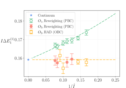
Figure 4: Linear $\theta$-correction to the first energy level, $\Delta E_{1}$, for a periodic lattice with the standard discretization of the action at different values of $\hat{I}$ with constant $T/I=20$. The results were obtained using the interpolating operator $O_{1}(t)=\phi_{t}$ with reweighting on a simulation with periodic boundary conditions (green, open circles), and using $O_{2}(t)=\sin(\phi_{t})$ with HAD (yellow, open squares) and reweighting (red, filled circles) with open and periodic boundary conditions, respectively. The dashed lines represent the corresponding the analytic results obtained with open boundary conditions (see section B.1).

V Conclusions

We have studied a well-known toy model of QCD to explore a recent claim to solve the strong CP problem, where it is argued that physical observables do not depend on the $\theta$ angle of QCD because the infinite volume limit should be taken before the summation over topological sectors, an order of limits which makes $\theta$ disappear from the energy spectrum of the theory. Concretely, the authors of refs. [6, 7] consider global observables (i.e. integrals over all spacetime), where the order of limits is indeed relevant and subtleties about the choice of boundary conditions have to be addressed with care. For the case of local observables, their claim is based on the requirement of topological quantization, which is usually seen in the limit of infinite spacetime.

In the present work we argue that quantities of physical interest that can be compared with experiment are intrinsically local and therefore their dependence on the choice of boundary conditions or global questions such as the quantization of the global topological charge are completely irrelevant. We have studied observables in the quantum rotor model from local correlators, and we have shown that the requirement of topological quantization at any finite value of the lattice spacing and volume is unimportant. In fact, we have seen that even in cases for which the topology is not quantized, the local correlators deliver the correct $\theta$-dependence of the observables.

Particularly we have determined the topological susceptibility and the spectrum of the theory from local correlators with different choices of boundary conditions (open and periodic), and also at fixed topological charge using volume averages on very large volumes (using master field simulations). We find perfect agreement in the $\theta$-dependence between all the methods and the analytical results.

For the computation of the $\theta$-dependence of the observables on the lattice we have studied two recent proposals that might yield a computational advantage with respect to the standard ways of alleviating the sign problem. These new proposals involve using truncated polynomials to automatically Taylor expand observables in $\theta$. These methods have the advantage that one can obtain the full dependence on the first orders of $\theta$ from a single simulation at $\theta=0$. Concretely, we have studied truncated polynomials using reweighting techniques and the HMC algorithm.

We conclude that at least for the quantities of physical interest that can be derived from local correlators, such as the susceptibility or the electric dipole moment of the neutron in the case of QCD, the order of limits is irrelevant, and a dependence on $\theta$ in the observables is still present. We still fail to understand why QCD decides to respect CP with such a high accuracy.

Aknowledgements

We specially want to thank C. Tamarit for his patience explaining to us the arguments of [6, 7], P. Hernandez for the extremely useful discussions, and S. Cruz-Alzaga for his contribution at the early stages of this work. We acknowledge support from the Generalitat Valenciana grant PROMETEO/2019/083, the European projects H2020-MSCA-ITN-2019//860881-HIDDeN and 101086085-ASYMMETRY, and the national project PID2020-113644GB-I00 as well as the technical support provided by the Instituto de Física Corpuscular, IFIC (CSIC-UV). DA acknowledges support from the Generalitat Valenciana grants ACIF/2020/011 and PROMETEO/2021/083. GC and AR acknowledge financial support from the Generalitat Valenciana grant CIDEGENT/2019/040. The computations were performed on the local SOM clusters, funded by the MCIU with funding from the European Union NextGenerationEU (PRTR-C17.I01) and Generalitat Valenciana, ASFAE/2022/020. We also acknowledge the computational resources provided by Finis Terrae II (CESGA), Lluis Vives (UV), Tirant III (UV). The authors also gratefully acknowledge the computer resources at Artemisa, funded by the European Union ERDF and Comunitat Valenciana, as well as the technical support provided by the Instituto de Física Corpuscular, IFIC (CSIC-UV).

Appendix A Analytical lattice two-point function with open boundary conditions

Consider the generating functional for correlation functions of the topological charge density on the lattice,

$$Z[J]=\int\left(\prod_{t=1}^{N}d\phi_{t}\right)\exp[-S(\phi)+\sum_{t=1}^{T/a}J_{t}q_{t}\bigg{]},$$ (33)

with the source $J_{t}$ and $q_{t}=\frac{1}{2\pi}(\phi_{t+1}-\phi_{t})\bmod 2\pi$. The explicit form of the discretized actions in eqs. 6 and 7 and topological charge in eqs. 8 and 9 depend only on the combination $\phi_{t+1}-\phi_{t}$. This suggests the change of integration variables $\phi_{t}\rightarrow q_{t}$ defined by

$$\phi_{t}=\phi_{\hat{T}-1}-\sum_{i=t}^{\hat{T}-1}q_{i},$$ (34)

with $t\in[0,\hat{T}-1]$ and $q_{\hat{T}-1}=0$. With open boundary conditions every time layer decouples leaving $\hat{T}-1$ identical independent integrals. For the case of the classical perfect action in eq. 6 we get

$$Z[J]=2\pi\left(-\sqrt{\frac{\pi}{2\pi}}\right)^{N}\prod_{i=1}^{N-1}e^{-\frac{\left(J_{i}+i\frac{\theta}{2\pi}\right)^{2}}{2\hat{I}}}$$ (35)

$$\times\left[\erf\left(\frac{-J_{i}-i\frac{\theta}{2\pi}-\pi\hat{I}}{\sqrt{2\hat{I}}}\right)+\erf\left(\frac{J_{i}+i\frac{\theta}{2\pi}-\pi\hat{I}}{\sqrt{2\hat{I}}}\right)\right].$$

Differentiating the functional integral with respect to $J_{t_{1}}$ and $J_{t_{2}}$ and setting these to zero gives us the connected two-point correlation function of the topological charge density,

$$\expectationvalue{q_{t_{1}}q_{t_{1}}}_{c}=\frac{1}{Z[0]}\evaluated{\frac{\delta^{2}Z[J]}{\delta J_{1}\delta J_{2}}}_{J=0}.$$ (36)

For a finite distance $t_{1}-t_{2}\neq 0$ the two-point function vanishes, while for $t_{1}=t_{2}$ we get

$$\expectationvalue{q_{t}q_{t}}_{c} =\frac{1}{4\pi^{2}\hat{I}}\Bigg{\{}1+\frac{\sqrt{2\hat{I}}}{\sqrt{\pi}C^{2}(\theta,\hat{I})}$$ (37)

$$\quad\times\Bigg{[}\frac{e^{-\frac{A^{2}(\hat{I},-\theta)}{2\hat{I}}}}{\hat{I}}\left(C(\theta,\hat{I})A(\hat{I},-\theta)-\hat{I}\sqrt{2/\pi}\right)$$

$$\quad+\frac{e^{-\frac{A^{2}(\hat{I},\theta)}{2\hat{I}}}}{\hat{I}}\left(C(\theta,\hat{I})A(\hat{I},\theta)+\hat{I}\sqrt{2/\pi}\right)\Bigg{]}\Bigg{\}},$$

where $A(\hat{I},\theta)\equiv\pi\hat{I}+\frac{i\theta}{2\pi}$ and

$$C(\theta,\hat{I})=\erf\left(\frac{-A(\hat{I},\theta)}{\sqrt{2\hat{I}}}\right)+\erf\left(\frac{-A(\hat{I},-\theta)}{\sqrt{2\hat{I}}}\right).$$ (38)

Eq. (37) gives the exact result of the correlation function for any value of $\hat{I}$ and $\theta$. Additionally, the continuum value is recovered for $\hat{I}\rightarrow\infty$. The complete lack of finite-$T$ effects is due to the choice of boundary conditions that effectively decouple the time layers.

The global definition of the topological susceptibility can also be computed from the above generating functional,

$$\chi_{t}(\theta)^{\text{global}} =-\frac{1}{T}\partialderivative[2]{\log Z[0]}{\theta}=\frac{T-1}{T}\expectationvalue{q_{t}q_{t}}_{c},$$ (39)

recovering a similar expression up to finite-$T$ effects.

Appendix B Spectrum and $\theta$-dependence from the lattice

B.1 Analytical results

The energy spectrum of the lattice theory can be computed analytically for different choices of the action discretization. We consider a Fourier transform of the transfer matrix [32] with respect to $\psi_{t}=\phi_{t+a}-\phi_{t}$,

$$A_{n}(\theta)\equiv e^{-aE_{n}{\theta}}=\int_{-\pi}^{\pi}d\psi\bra{\phi_{t+a}}\mathcal{T}\ket{\phi_{t}}e^{-in\psi}.$$ (40)

The transfer matrix for the standard discretization of the action and topological charge of the action and topological charge reads

$$\bra{\phi_{t+a}}\mathcal{T}\ket{\phi_{t}}_{\rm{st}}=\sqrt{\frac{\hat{I}}{2\pi}}\exp\{-\hat{I}(1-\cos\psi)+i\frac{\theta}{2\pi}\sin\psi\bigg{\}},$$ (41)

and the corresponding energies are

$$e^{-E_{n}}=\sqrt{\frac{\hat{I}}{2\pi}}\int_{-\pi}^{\pi}d\psi\,\exp{-\frac{\hat{I}}{a}(1-\cos\psi)}$$

$$\times\exp{in\psi-i\frac{\theta}{2\pi}\sin\psi}$$ . (42)

For the classical perfect discretization the transfer matrix is

$$\bra{\phi_{t+a}}\mathcal{T}\ket{\phi_{t}}_{\rm{cp}}$$ (43)

$$\begin{aligned} \quad=\sqrt{\frac{\hat{I}}{2\pi}}\exp\{&-\frac{\hat{I}}{2}((\phi_{t+1}-\phi_{t})\bmod 2\pi)^{2}\\ &+i\frac{\theta}{2\pi}(\phi_{t+1}-\phi_{t})\bmod 2\pi\bigg{\}},\end{aligned}$$

and the energies read

$$e^{-E_{n}}=\sqrt{\frac{\hat{I}}{2\pi a}}\int_{-\pi}^{\pi}d\psi\,\exp{-\frac{\hat{I}}{2}\psi^{2}+i\psi\left(n-\frac{\theta}{2\pi}\right)}.$$ (44)

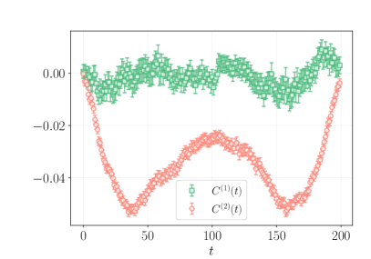
Figure 5: Linear (green squares) and quadratic (red circles) contributions to the two-point function $C(t)=\expectationvalue{\phi_{t}\phi_{0}}_{c}$ in the $\theta$-expansion from a simulation at $\hat{I}=10$ and $\hat{T}=200$ with periodic boundary conditions and the standard action.

B.2 Lattice correlators

The correlation functions on a finite lattice are modified due to the choice of boundary conditions. For a periodic lattice, each term $k$ in LABEL:eq:spectraldecomposition_correlator has an additional contribution $e^{-(T-t)\Delta E_{k}}$. Its behavior at large $t$ is modified to

$$C(t) =2Ae^{-\Delta E_{1}^{(1)}t}\left[1+\left(\Delta E_{1}^{(0)}t\theta\right)^{2}\right]$$ (45)

$$+2Ae^{-\Delta E_{1}^{(1)}(T-t)}\left[1+\left(\Delta E_{1}^{(0)}(T-t)\theta\right)^{2}\right],$$

where we used $\Delta E_{1}^{(1)}=-\Delta E_{-1}^{(1)}$. To extract the linear correction to the energy we consider the ratio

$$\frac{C^{(2)}(t)}{C^{(0)}(t)}=\frac{1}{2}(\Delta E_{1}^{(1)})^{2}\left[t^{2}+\frac{(T^{2}-2tT)}{1+e^{-\Delta E_{1}^{(0)}(T-2t)}}\right].$$ (46)

In fig. 5 the two first contributions to the two-point correlator $\expectationvalue{\phi_{t}\phi_{0}}_{c}$ in the $\theta$ expansion are shown for a periodic lattice for a simulation with the standard dicretization of the action using periodic boundary conditions. The linear term is compatible with zero, as expected from eq. (45). The ratio in eq. 46 is plotted in fig. 6. The fit is shown to match the exact value for this discretization obtained with the functional form in eq. 46 and the energy values from section B.1.

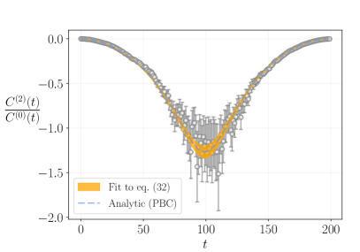
Figure 6: Ratio $C^{(2)}(t)/C^{(0)}(t)$ from a simulation at $\hat{I}=10$ and $\hat{T}=200$ with periodic boundary conditions using the standard action. The resulting fit with the functional form in LABEL:eq:ratio_correlatorPBC is shown (yellow band) together with the exact analytical result (blue dashed line).

Appendix C Winding transformation

We define the winding transformation on a quantum rotor configuration as

$$\mathcal{W}^{\pm}:\,\phi_{t}\to\phi_{t}^{\mathcal{W}^{\pm}}=\phi_{t}\pm 2\pi t/\hat{T},$$ (47)

for $t\in[0,\hat{T}-1]$. Assuming a smooth enough configuration $\phi$ such that $(\phi_{t+1}-\phi_{t}\bmod 2\pi)\pm 2\pi/\hat{T}\in[-\pi,\pi)$ —which is the case close enough to the continuum—, one can show that the winding transformation changes its classical topological charge in one unit, i.e.

$$Q_{\text{cp}}(\phi^{\mathcal{W}^{\pm}})=Q_{\text{cp}}(\phi)\pm 1.$$ (48)

The change in the classical perfect action after the winding transformation is

$$\Delta S_{\text{cp}}^{\mathcal{W}^{\pm}}\equiv \,S_{\text{cp}}(\phi^{\mathcal{W}^{\pm}})-S_{\text{cp}}(\phi)$$

$$= \,2\pi^{2}\left(1\pm 2Q_{\text{cp}}(\phi)\right)\frac{\hat{I}}{\hat{T}},$$ (49)

and can be made small by increasing the time extent $\hat{T}$ of the lattice. One can use this transformation to propose new samples in a Metropolis algorithm, to be accepted with probability

$$p_{\text{acc}}(\phi^{\mathcal{W}^{\pm}}\mid\phi)=\min\left\{1,\exp(-\Delta S_{\text{cp}}^{\mathcal{W}^{\pm}})\right\}.$$ (50)

Note that one must use this update step in combination with other sampling algorithm to ensure ergodicity [16].

References

- Chupp et al. [2019] T. E. Chupp, P. Fierlinger, M. J. Ramsey-Musolf, and J. T. Singh, Electric dipole moments of atoms, molecules, nuclei, and particles, Rev. Mod. Phys. 91, 015001 (2019).
- Aoki et al. [2022] Y. Aoki et al. (Flavour Lattice Averaging Group (FLAG)), FLAG Review 2021, Eur. Phys. J. C 82, 869 (2022), arXiv:2111.09849 [hep-lat] .
- Peccei and Quinn [1977] R. D. Peccei and H. R. Quinn, Constraints imposed by conservation in the presence of pseudoparticles, Phys. Rev. D 16, 1791 (1977).
- Nelson [1984] A. E. Nelson, Naturally Weak CP Violation, Phys. Lett. B 136, 387 (1984).
- Barr [1984] S. M. Barr, Solving the strong problem without the peccei-quinn symmetry, Phys. Rev. Lett. 53, 329 (1984).
- Ai et al. [2021a] W.-Y. Ai, J. S. Cruz, B. Garbrecht, and C. Tamarit, Absence of $CP$ violation in the strong interactions, Physics Letters B 822, 136616 (2021a), arXiv:2001.07152 [hep-ph, physics:hep-th].
- Ai et al. [2021b] W.-Y. Ai, J. S. Cruz, B. Garbrecht, and C. Tamarit, Consequences of the order of the limit of infinite spacetime volume and the sum over topological sectors for CP violation in the strong interactions, Physics Letters B 822, 136616 (2021b).
- Shindler et al. [2015] A. Shindler, T. Luu, and J. de Vries, Nucleon electric dipole moment with the gradient flow: The -term contribution, Phys. Rev. D 92, 094518 (2015), arXiv:1507.02343 [hep-lat] .
- Dragos et al. [2021] J. Dragos, T. Luu, A. Shindler, J. de Vries, and A. Yousif, Confirming the Existence of the strong CP Problem in Lattice QCD with the Gradient Flow, Phys. Rev. C 103, 015202 (2021), arXiv:1902.03254 [hep-lat] .
- Giusti and Lüscher [2019] L. Giusti and M. Lüscher, Topological susceptibility at from master-field simulations of the SU(3) gauge theory, Eur. Phys. J. C 79, 207 (2019), arXiv:1812.02062 [hep-lat] .
- Lüscher [2018] M. Lüscher, Stochastic locality and master-field simulations of very large lattices, EPJ Web Conf. 175, 01002 (2018), arXiv:1707.09758 [hep-lat] .
- Alles et al. [1996] B. Alles, G. Boyd, M. D’Elia, A. Di Giacomo, and E. Vicari, Hybrid Monte Carlo and topological modes of full QCD, Phys. Lett. B 389, 107 (1996), arXiv:hep-lat/9607049 .
- Del Debbio et al. [2002] L. Del Debbio, H. Panagopoulos, and E. Vicari, theta dependence of SU(N) gauge theories, JHEP 08, 044, arXiv:hep-th/0204125 .
- Del Debbio et al. [2004] L. Del Debbio, G. M. Manca, and E. Vicari, Critical slowing down of topological modes, Phys. Lett. B 594, 315 (2004), arXiv:hep-lat/0403001 .
- Schaefer et al. [2011] S. Schaefer, R. Sommer, and F. Virotta (ALPHA), Critical slowing down and error analysis in lattice QCD simulations, Nucl. Phys. B 845, 93 (2011), arXiv:1009.5228 [hep-lat] .
- Albandea et al. [2021] D. Albandea, P. Hernández, A. Ramos, and F. Romero-López, Topological sampling through windings, The European Physical Journal C 81, 10.1140/epjc/s10052-021-09677-6 (2021).
- de Forcrand [2009] P. de Forcrand, Simulating QCD at finite density, PoS LAT2009, 010 (2009), arXiv:1005.0539 [hep-lat] .
- Gattringer and Langfeld [2016] C. Gattringer and K. Langfeld, Approaches to the sign problem in lattice field theory, Int. J. Mod. Phys. A 31, 1643007 (2016), arXiv:1603.09517 [hep-lat] .
- Bhanot and David [1985] G. Bhanot and F. David, The Phases of the O(3) Model for Imaginary , Nucl. Phys. B 251, 127 (1985).
- Azcoiti et al. [2002] V. Azcoiti, G. Di Carlo, A. Galante, and V. Laliena, New proposal for numerical simulations of theta vacuum - like systems, Phys. Rev. Lett. 89, 141601 (2002), arXiv:hep-lat/0203017 .
- Alles and Papa [2008] B. Alles and A. Papa, Mass gap in the 2D O(3) non-linear sigma model with a theta=pi term, Phys. Rev. D 77, 056008 (2008), arXiv:0711.1496 [cond-mat.stat-mech] .
- Alles et al. [2014] B. Alles, M. Giordano, and A. Papa, Behavior near of the mass gap in the two-dimensional O(3) non-linear sigma model, Phys. Rev. B 90, 184421 (2014), arXiv:1409.1704 [hep-lat] .
- Panagopoulos and Vicari [2011] H. Panagopoulos and E. Vicari, The 4D SU(3) gauge theory with an imaginary term, JHEP 11, 119, arXiv:1109.6815 [hep-lat] .
- D’Elia and Negro [2012] M. D’Elia and F. Negro, dependence of the deconfinement temperature in Yang-Mills theories, Phys. Rev. Lett. 109, 072001 (2012), arXiv:1205.0538 [hep-lat] .
- Bonati et al. [2016a] C. Bonati, M. D’Elia, and A. Scapellato, dependence in Yang-Mills theory from analytic continuation, Phys. Rev. D 93, 025028 (2016a), arXiv:1512.01544 [hep-lat] .
- Aoki et al. [2008] S. Aoki, R. Horsley, T. Izubuchi, Y. Nakamura, D. Pleiter, P. E. L. Rakow, G. Schierholz, and J. Zanotti, The Electric dipole moment of the nucleon from simulations at imaginary vacuum angle theta, (2008), arXiv:0808.1428 [hep-lat] .
- Bonati et al. [2016b] C. Bonati, M. D’Elia, P. Rossi, and E. Vicari, dependence of 4D gauge theories in the large- limit, Phys. Rev. D 94, 085017 (2016b), arXiv:1607.06360 [hep-lat] .
- Bonanno et al. [2023] C. Bonanno, M. D’Elia, and L. Verzichelli, The -dependence of the critical temperature at large , (2023), arXiv:2312.12202 [hep-lat] .
- Bonanno et al. [2024] C. Bonanno, C. Bonati, M. Papace, and D. Vadacchino, The -dependence of the yang-mills spectrum from analytic continuation (2024), arXiv:2402.03096 [hep-lat] .
- Catumba et al. [2023] G. Catumba, A. Ramos, and B. Zaldivar, Stochastic automatic differentiation for Monte Carlo processes, (2023), arXiv:2307.15406 [hep-lat] .
- Fjeldso et al. [1987] N. Fjeldso, J. Midtdal, and F. Ravndal, Random walks of a quantum particle on a circle, (1987).
- Bietenholz et al. [1997] W. Bietenholz, R. Brower, S. Chandrasekharan, and U.-J. Wiese, Perfect Lattice Topology: The Quantum Rotor as a Test Case, Physics Letters B 407, 283 (1997), arXiv:hep-lat/9704015.
- Manton [1980] N. S. Manton, An alternative action for lattice gauge theories, Phys. Lett. B 96, 328 (1980).
- Duane et al. [1987] S. Duane, A. Kennedy, B. J. Pendleton, and D. Roweth, Hybrid monte carlo, Physics Letters B 195, 216 (1987).
- Brida and Lüscher [2017] M. D. Brida and M. Lüscher, SMD-based numerical stochastic perturbation theory, Eur. Phys. J. C 77, 308 (2017), arXiv:1703.04396 [hep-lat].
- Coleman [1985] S. Coleman, Aspects of Symmetry: Selected Erice Lectures (Cambridge University Press, 1985).
- Metropolis et al. [1953] N. Metropolis, A. W. Rosenbluth, M. N. Rosenbluth, A. H. Teller, and E. Teller, Equation of state calculations by fast computing machines, J. Chem. Phys. 21, 1087 (1953).
- Ramos [2023] A. Ramos, Formalseries.jl (2023), https://igit.ific.uv.es/alramos/formalseries.jl.
- Haro [2011] A. Haro, Automatic differentiation tools in computational dynamical systems, (2011).
- Di Renzo et al. [1994] F. Di Renzo, G. Marchesini, P. Marenzoni, and E. Onofri, Lattice perturbation theory on the computer, Nucl. Phys. B Proc. Suppl. 34, 795 (1994).
- Dalla Brida and Lüscher [2017] M. Dalla Brida and M. Lüscher, SMD-based numerical stochastic perturbation theory, Eur. Phys. J. C 77, 308 (2017), arXiv:1703.04396 [hep-lat] .