Solitary cluster waves in periodic potentials: Formation, propagation, and soliton-mediated particle transport
Abstract
Transport processes in crowded periodic structures are often mediated by cooperative movements of particles forming clusters. Recent theoretical and experimental studies of driven Brownian motion of hard spheres showed that cluster-mediated transport in one-dimensional periodic potentials can proceed in form of solitary waves. We here give a comprehensive description of these solitons. Fundamental for our analysis is a static presoliton state, which is formed by a periodic arrangements of basic stable clusters. Their size follows from a geometric principle of minimum free space. Adding one particle to the presoliton state gives rise to solitons. We derive the minimal number of particles needed for soliton formation, number of solitons at larger particle numbers, soliton velocities and soliton-mediated particle currents. Incomplete relaxations of the basic clusters are responsible for an effective repulsive soliton-soliton interaction seen in measurements. Our results provide a theoretical basis for describing experiments on cluster-mediated particle transport in periodic potentials.
I Introduction
Particle transport in densely populated periodic structures frequently proceeds by cooperative movements of particle assemblies. Examples are surface crowdions in copper adatom diffusion on a strained surface [1], interstitial crowdions in crystals [2, 3], and similar types of vacancy clusterings in form of anti-crowdions [4] or voidions [5, 6]. A further example are defect motions in colloidal monolayers, which are completely filled wells of a two-dimensional periodic or quasi-periodic optical potential [7, 8, 9, 10, 11, 12]. Under time-dependent forcing, cluster-mediated transport was seen for vortices in a nanostructured superconducting film driven by an oscillating electric current [13], paramagnetic colloids above a magnetic bubble lattice driven by a rotating magnetic field [14, 15, 16], and polystyrene particles driven by an oscillating periodic optical potential [17].
In various of these studies [8, 18, 10, 11, 6, 12], aspects of the cooperative particle dynamics could be successfully interpreted by resorting to the physics of the Frenkel-Kontorova (FK) model [19]. This model allows for the formation of solitary waves. When charged colloidal particles in periodic potentials are sliding under a viscous drag force, double occupied and vacant wells in chains of single-occupied wells act as kinks (local compression) and antikinks (local expansion) [8] as in the FK model. Similarity to the dynamics in the FK model was further demonstrated by Newtonian dynamics simulations of these experiments [10]. In simulations of defective crystals, particle displacements within extended defects created by a vacancy (voidions) or interstitial (crowdions) could be described by solutions of the sine-Gordon equation, which corresponds to a continuum limit of the FK model.
Different solitary waves of particle clusters were predicted to occur in overdamped Brownian motion of hard spheres through one-dimensional periodic potentials [20]. Particle currents mediated by these solitons at low temperature showed pronounced peaks at certain magic hard-sphere diameters. This was found when the number of particles exceeds the number of potential wells by one.
Recently, the novel solitary cluster waves were observed in experiments [21]. They uncovered new fundamental features of the soliton dynamics: the formation of multiple cluster waves when the overfilling
| (1) |
of the potential wells is larger than one, and indications of a repulsive soliton-soliton interaction in the multi-soliton states.
These findings await an explanation. Generally, a number of questions arises:
-
Will solitary cluster waves appear for all particle diameters, if the overfilling of potential wells is sufficiently high?
-
Is there a minimal overfilling needed to create cluster solitons?
-
How does the number of solitons vary with the overfilling ?
-
What is the nature of the experimentally observed interaction between cluster solitons?
-
How are particle currents related to solitary cluster waves?
We will tackle these questions in this study. Our answers provide a basic understanding of cluster-mediated particle transport in periodic potentials.
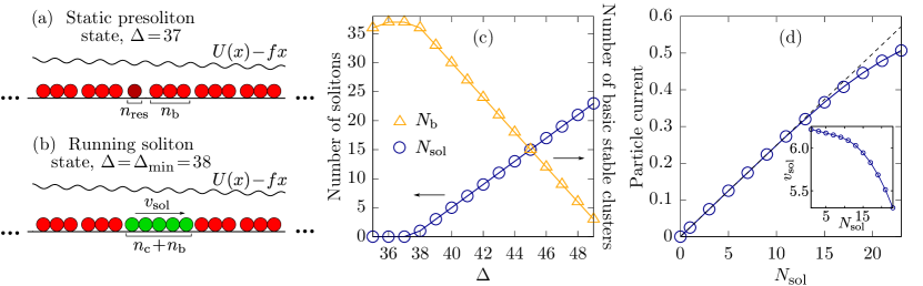
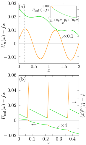
Figure 1 gives an overview of key physical mechanisms and concepts that we will discuss. Fundamental is the characterization of the presoliton state in Fig. 1(a), which shows a periodic arrangement of mechanically stable particle clusters in a tilted periodic energy landscape , where is a drag force. The presoliton state arises when increasing the particle number until a further addition of a particle leads to a running state carrying one or more solitons, see Fig. 1(b). In the example shown in the figure, the presoliton is reached for overfilling and one soliton appears after adding one particle, i.e. at the minimal overfilling for soliton formation. Movie 1 of the Supplemental Material (SM) [22] shows the soliton motion for the single-soliton state.
In the dynamical phase transition from the presoliton to the running state, the number of solitons jumps from for to at , see Fig. 1(c). For , increases linearly with with slope two, i.e. two further solitons are created per added particle. The soliton-mediated particle current in the stationary state in Fig. 1(d) is proportional to the soliton number for small , but the increase with becomes sublinear for large . This is a consequence of a slowing-down of the soliton’s velocity with , see the inset of Fig. 1(d). The slowing down corresponds to an effective repulsive soliton-soliton interaction.
II Solitary cluster waves
We consider particles dragged by a constant force across a sinusoidal potential, for which first experimental observations of the solitary waves were reported in Ref. [21]. The particles’ motion is described by the Langevin equations
| (2) |
where , , are the particle positions, is the bare mobility, is the diffusion coefficient, is the thermal energy, and are Gaussian white noise processes with zero mean and correlation functions . The hard-sphere interaction constrains the particle distances to
| (3) |
where is the particle diameter. The periodic potential is
| (4) |
where is the wavelength and is the barrier between neighboring potential wells.
With increasing drag force , the barriers of the tilted potential become smaller. They disappear at the critical force
| (5) |
for overtilting.
The dynamics of the particles is constrained to a finite interval of size with periodic boundary conditions, where is an integer multiple of . We set in the following, and use , and as units of energy, length and time, respectively.
In our previous work [20], we treated a special case of particle diameters in the range for overfilling , i.e. when the number of particles exceeds the number of potential wells by one. For high barriers of the periodic potential and weak drag force , we found that particle currents as a function of exhibit peaks at magic particle diameters , Solitary cluster waves, which manifest themselves as periodic sequences of cluster movements, are responsible for this striking behavior. Their properties could be derived by considering the limit of zero noise, where Eqs. (2) are
| (6) |
The situation becomes much more complex when considering arbitrary overfillings and particle diameters . In this study we tackle this problem based on Eqs. (6) and derive general conditions for the appearance of solitons and describe their properties.
We first give in Sec. III basic features of particle clusters in a tilted periodic potential. In Sec. IV we discuss presoliton states, which are mechanically stable states with largest number of particles. The presoliton state is formed by basic mechanically stable clusters composed of particles. The knowledge of allows us to derive in Sec. V the minimal overfilling necessary to generate solitons. In Sec. VI we describe how solitons propagate by periodic sequences of cluster movements and derive their time period and velocity. Thereafter we analyze in Sec. VII how many solitons form for a given overfilling and discuss in Sec. VIII how our results can be tested in experiments. We explain the effective repulsive soliton-soliton interaction in Sec. IX and derive the particle currents mediated by solitons in Sec. X.
Our analysis is performed for hard-sphere diameters . Section XI discusses how results for larger than the wavelength are obtained from those for .
When referring to simulations, these are carried out by applying the recently developed method of Brownian cluster dynamics [23].
III Particle clusters in tilted periodic potential
An -cluster is formed by particles in contact, i.e. with positions , . We define the position of the -cluster as the position of the first particle, . An -cluster has size in terms of number of particles and it covers an interval of size .
If the particles in the -cluster keep in contact, the mean force acting on it is , where
| (7) |
is the -cluster potential. For the magic particle diameters , , i.e. an -cluster with particles of diameter moves without surmounting barriers if the particles in the cluster stay together during the motion.
Particles in an -cluster at position keep in contact if the non-splitting conditions
| (8) |
are obeyed, where is the force acting on a single particle; note that cancels in these conditions. The conditions mean the following: when considering any decomposition of the -cluster into an -subcluster and -subcluster at its left and right end, respectively, the velocity of (or force on) the -subcluster must be larger than that of the -subcluster, i.e. the subclusters do not separate.
If the non-splitting conditions are satisfied, the -cluster at position has the velocity ()
| (9) |
If they are satisfied in an interval , the time for the -cluster to move from to is
| (10) |
The tilted potential has barriers if the force is smaller than the critical force
| (11) |
for overtilting of the -cluster potential. For a single-particle, , with from Eq. (5). An -cluster can be mechanically stable only for .
It is mechanically stable if it is at a position , where has a local minimum,
| (12) |
and if the -cluster does not fragment, i.e. if the non-splitting conditions (8) are obeyed.
IV Presoliton states
The presoliton state is the state of stable mechanical equilibrium with the largest number of particles. Simulations starting from different initial particle configurations show that it is formed by a sequence of evenly separated clusters with the same particle number and a residual of particles, see Fig. 1(a), where ; is also possible. We call the basic stable cluster size and an -cluster a basic one. It will play a fundamental role in the following.
In Sec. IV.1, we first derive for the case of infinitesimal force , which we refer to as zero-force limit. In this limit, solitons can occur only if the particle diameter is a rational number (in units of the wavelength ,
| (15) |
This is a necessary condition, since for such , see Eq. (7), i.e. a -cluster could move without surmounting barriers. To represent each such uniquely, and are taken to be coprime. Because , it is .
The necessary condition does not imply that solitons must occur for all . For example, in Ref. [20] solitons were studied for overfilling and appeared for only. We will show that solitons occur for most , if the overfilling exceeds a minimal value . This The required minimal overfilling is calculated in Sec. V. It may, however, not be realizable for a finite system size .
The knowledge for allows us to determine for finite also, which we show in Sec. IV.2.
IV.1 Basic stable cluster size for
For an -cluster to be in stable mechanical equilibrium, it must be placed at a local minimum of the effective potential [Eq. (7)] and it must not split [conditions (8)]. We refer to these two conditions as translation stability and fragmentation stability. If both conditions are met, we call an -cluster stable. An -cluster is called stabilizable, if it is stable against fragmentation at a position of a local minimum of .
A 1-cluster (single particle) is stabilizable, as it cannot fragment. Clusters of size are unstable, because has no local minimum. A cluster of size is unstable also. This is because it can be divided into two subclusters, one to the left of size , and one to the right of size . The right -subcluster moves in the presence of an infinitesimal force and the left subcluster of size can only speed up the motion of the right -subcluster. Hence, a cluster in stable mechanical equilibrium must have a size smaller than . We conclude that .
Interestingly, stabilizability of a cluster is related to a geometric property, which is the residual free space when the cluster is accommodated in a minimal number of potential wells. Specifically, we define the residual free space of an -cluster as the difference between the space covered by accommodating potential wells ( wavelengths) and the space covered by the cluster:
| (16) |
Here, is the smallest integer larger than .
The relation between stabilizability and residual free space is given by the following free-space theorem, derived in Appendix A: If an isolated -cluster is stabilizable, its residual free space is smaller than that of any cluster of smaller size, i.e. it holds
| (17) |
It follows that the largest among the stabilizable clusters has smallest residual free space. This is because for any two stabilizable - and -clusters with sizes , it holds according to Eq. (17).
The cluster with minimal residual free space is unique, i.e. the are all different for . To show this, let us assume that there exist with and , i.e. . This would imply that is an integer. However, this is impossible for coprime and , and . In particular, we obtain
| (18) |
A mechanically stable state with largest particle number has highest coverage . The highest coverage is obtained, if successive potential wells accommodate a largest stabilizable cluster with minimal residual free space. Accordingly, is determined from a principle of minimum residual free space:
| (19) |
Equivalently, is determined by Eq. (18), i.e. . This condition can be rewritten in the form
| (20) |
where .
For being an arbitrary integer, Eq. (20) is a linear Diophantine equation in the two variables and . Its solutions are [24]
| (21) | ||||
| (22) |
where can be any integer , is Euler’s Phi function [25] and is an integer due to the Euler-Fermat theorem [24]. Because , the integer in Eq. (21) must be . We hence obtain the explicit solution
| (23) |
The gives also the required :
| (24) |
Here we have used for integer and . The last equality in Eq. (24) follows when inserting into Eq. (22). Let us note also that Eq. (20) implies that and must be coprime.

Figure 2 shows representative results of for in dependence of for (a) and (b) . They exhibit a recurrent behavior with a period , where increases linearly with with a slope that is an integer multiple of , see the dashed lines.
We note that can be equal to one, which means that all -clusters with are mechanically unstable. A particular set of particle diameters with is given by . For , .
IV.2 Basic stable cluster size for
For drag forces , the largest translational stable cluster has size
| (25) |
where the critical force for overtilting is given in Eq. (11). This limits the range of stabilizable clusters.
Interestingly, our simulations show that Eq. (17) remains valid for , with replacing . Hence the residual free space of a stabilizable cluster with size is smaller than that of clusters with size . Similarly as in Eq. (19),
| (26) |
where .
Equations (25) and (26) imply that can be determined for any and by the following method: First one checks whether an -cluster, with from Eq. (25), is stabilizable by using Eq. (8). If it is not stabilizable, is decreased by one and the stabilizability of this -cluster is checked. The procedure is repeated until the cluster of size is stabilizable. This is equal to , since by decreasing the cluster size, the residual free space increases.
V Minimal overfilling
Knowing , the minimal overfilling for soliton appearance follows from geometric considerations. In the presoliton state, the maximal number of stable -clusters fitting into a system of length is
| (27) |
The number of potential wells accommodating all -clusters is
| (28) |
There can be residual potential wells not accommodating -clusters. Their number is
| (29) |
where denotes the modulo operation. The number of particles fitting into the residual wells is
| (30) |
Accordingly, the maximal particle number in a configuration of stable mechanical equilibrium is
| (31) |
Adding one more particle gives rise to a soliton, i.e.
| (32) | ||||
However, the coverage by the particles must not exceed the system length ,
| (33) |
If this self-consistency condition is not fulfilled, solitons do not form.
Let us discuss a few examples for the case of weak forces, where solitons can only occur when is close to . We therefore consider the zero-force limit .
For a particle diameter and a system size , and 3/5 for , and 4. Hence , i.e. the minimum free space in accommodating potential wells is obtained for cluster size three. This is in agreement with Eq. (23). Hence, from Eq. (27), from Eq. (28), from Eqs. (29), (30), from Eq. (31), yielding according to Eq. (32). The self-consistency condition (33) reads and is satisfied.
The particle size and system size give an example, where not all particles are part of -clusters in the presoliton state. Here , , and , which satisfies the self-consistency condition (33).
An example, where soliton formation is impossible in a system of size is, when the particles have diameter . In that case, and , which violates the self-consistency condition (33), .
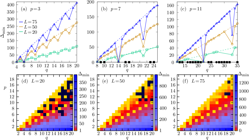
Figure 3 shows the minimal overfilling for soliton appearance for different and . In simulations we have verified both the absence of soliton formation and the values predicted by Eq. (32).
Figures 3(a)-(c) show the dependence of when varying at fixed , 7, and 11 for system sizes , 50 and 75. As a function of , shows an alternating behavior of increase and decrease with an overall linear increase, where the slope of the linear dependence rises with . Equation (32) predicts an overall behavior , i.e. the slope should be . The dashed lines in Fig. 3(a)-(c) representing indeed capture the overall linear increase of with .
Remarkable are the particle diameters for and where no solitons form for small drag force . At these particle diameters, there is not enough free space left to generate a soliton by adding one particle to the presoliton state. These states of soliton absence are represented by black squares in Figs. 3(e)-(f), where is plotted in a color-coded representation for a section of the -grid and three different system sizes [Fig. 3(e)], [Fig. 3(d)], and [Fig. 3(f)]. Theoretical results in Fig. 3 were checked against simulations.
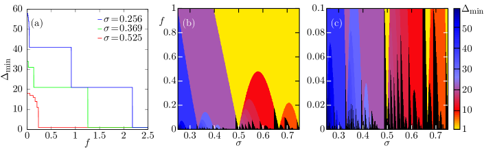
To exemplify the behavior of for a wide range of particle diameters and drag forces, we have carried out extensive simulations for a system of size . The results are displayed in Fig. 4(a)-(c), where in the color-coded representation of Fig. 4(b) a resolution and was chosen. Figure 4(c) depicts the region with small -values enlarged. For hundred randomly chosen points in the --plane in Fig. 4(b), we in particular checked that the simulated values agree with the predicted ones according to the algorithmic procedure described after Eq. (26).
Figure 4(a) shows how changes with for three fixed and . The overfilling at small is larger for smaller . With increasing , decreases in a stepwise manner, with the steps occurring at different for different . For large , becomes one for all .
A complete picture of soliton formation in the range and is given in Fig. 4(b). It has a remarkable complex structure, where black color marks soliton absence. At fixed , can change often between small and large values when is varied. The black areas occur at small , meaning that solitons formation requires a minimal for non-magic . Figure 4(c) is a zoom-in of the region , revealing a fractal-like pattern. When increasing , the black area becomes smaller and it vanishes for .
VI Soliton propagation
VI.1 Propagation modes
A soliton propagates by a sequential movement of clusters formed by splitting (detachment) and merging (attachment) events. There are two propagation modes, the basic one A and a variant B. Whether one or the other mode occurs, depends on and . The variant of the basic mode is less frequently encountered, in particular for . Both modes can be described by two clusters, the core soliton cluster of size , and the composite soliton cluster of size . Among the clusters involved in the soliton propagation, the core cluster has smallest size.
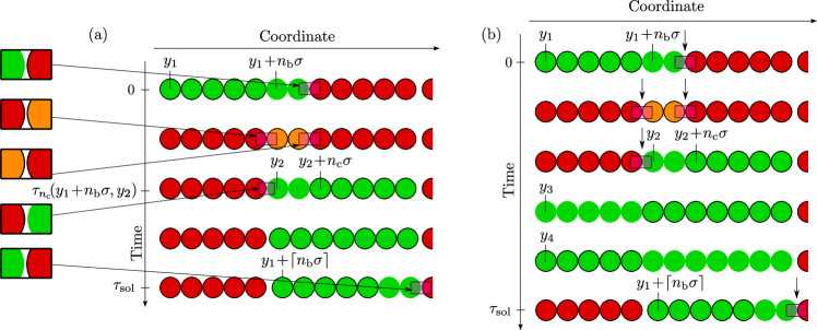
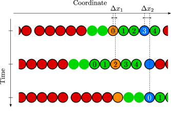
Figure 5(a) illustrates the basic mode A: when a composite -cluster terminates its movement at a position , an -cluster detaches at its right end, leaving an -cluster behind. After the detachment, the -cluster starts to relax towards a position of stable mechanical equilibrium, and the -cluster moves until reaching a position , where it attaches to an -cluster. The composite -cluster formed by the attachment moves until reaching a position . This completes one period of the soliton propagation: at the position equivalent to , the -cluster terminates its movement, because an -cluster detaches at its right end. Accordingly, a soliton moves a distance in one period.
In the variant B of the basic propagation mode, the relaxing -cluster is attaching to and shortly after detaching from the composite cluster, see Fig. 5(b). This slight modification of the basic propagation mode only occurs if at the time instant of the composite cluster formation, the distance between the right end of the relaxing -cluster and the left end of the composite cluster is very small and the relaxing cluster moves faster than the composite cluster. In the short intermediate time interval between detachment and attachment of the -cluster, the soliton propagation is mediated by an -cluster.
Movie 2 in the SM [22] shows the soliton propagation for modes A and B described in Figs. 5(a) and (b). The small change of from 0.57 to 0.5725 changes the soliton mode but not the cluster sizes and . In such cases, the soliton velocity is significantly larger for the B mode, as can be seen also in the movie.
In what follows, we focus on the basic propagation mode A. Quantities like soliton potentials or velocities discussed below can be treated analogously for the variant B. For the velocity of type B solitons, we give the corresponding calculation in Appendix B.
For weak drag force , or, strictly speaking in the zero-force limit, the composite cluster has size , i.e. it is the cluster that can move without surmounting barriers. This in particular implies that and are coprime, see comment after Eq. (24). The core soliton cluster then has size
| (34) |
The motion of the -cluster, however, does not span a full wavelength of the potential. This is because it splits into an - and -cluster at some point, which is in Fig. 5(a). At this point, the non-splitting conditions (8) are violated.
For larger , the core cluster can have a size smaller than . Other than in the case, where is constant for , it is possible that neither the core nor the composite cluster are able to move over one period, even if the non-splitting conditions were obeyed everywhere. This is demonstrated in Fig. 6(a), where we show the two tilted cluster potentials and of the core and composite cluster for and . Both tilted cluster potentials exhibit barriers, i.e. neither of the two soliton clusters could move over a full wavelength.
Due to the phase shift of the two cluster potentials, the barriers occur at different points. This enables the two soliton clusters to move over consecutive intervals of the period, where the forces and in each interval are positive and the non-splitting conditions (8) are fulfilled. One may view this as in a relay race, where the relay is passed between and -clusters.
As is known, it is possible to calculate based on the tilted cluster potentials: one needs to determine that , where the total force acting on an -cluster in one part of the period and on an -cluster in the other part of the period is positive and where the non-splitting conditions (8) in both parts are satisfied. This is equal to . For , this gives [26]
| (35) | ||||
with for and for .
We show below, see Eq. (50), that has a value giving coprime and .
VI.2 Soliton potential and force field
Taking the soliton position as that of the soliton clusters, i.e. the position of the leftmost particle of the - and -clusters in the basic propagation mode, we can define a potential for the soliton motion for :
| (36) |
Here, is the Heaviside step function [ for and zero otherwise]. The constants and were subtracted from the cluster potentials to make the soliton potential continuous at . That way, the force on the soliton jumps at from to , but has no -function singularity. The tilted soliton potential is shown in the inset of the figure, where the parts stemming from the core and composite soliton clusters are marked as in the main figure.
When a soliton starting at has moved one time period , its position jumps from to . After the jump, the potential is the same as at the starting position. For displaying the soliton potential, it is helpful to use a continuous-coordinate representation also with a coordinate , where the jumps in the real soliton coordinate are removed. In this representation, the soliton potential is periodic with a period length equal to the residual free space of the basic stable cluster.
Figure 6(b) shows the tilted soliton potential from the inset of Fig. 6(a) in the continuous-coordinate representation, and the corresponding force field . The force is always positive and it jumps when a core cluster attaches to a composite cluster. This corresponds to changes of the color from orange to green. When the color changes from green to orange, a core cluster detaches from a composite cluster. In such detachments events, the real soliton coordinate jumps by . These jumps are not visible in the continuous-coordinate representation in Fig. 6(b).
VI.3 Soliton velocity
The time period of the soliton motion is
| (37) |
where is the time for an -cluster to move from to given in Eq. (10).
The position is determined by the requirement that the -cluster detaches from the -cluster, i.e. the nonsplitting conditions (8) for the composite -cluster are violated for :
| (38) |
If the system size is large enough (limit ), the -clusters have enough time to relax to their positions of mechanical equilibria. One can then set approximately equal to from Eq. (13), with and the smallest integer satisfying . This gives
| (39) |
The mean soliton velocity is the distance travelled in a time period divided by ,
| (40) |
The corresponding expression for the type B mode of soliton motion is given in Appendix B.
An accurate treatment requires to consider the relaxation of the -clusters towards positions of stable mechanical equilibria. This will be discussed further below in Sec. IX in connection with an effective soliton-soliton interaction.
VII Number of solitons
If fulfills the inequality (33), solitons can occur for overfillings up to a maximal value satisfying , i.e.
| (41) |
The number of solitons increases with the overfilling and the minimal number can be larger than one.
For determining , we consider the presoliton state with . It is composed of clusters of the basic size and residual particles. By adding one particle, the presoliton state rearranges into a nonequilibrium steady state, where a maximal number of stable -clusters remains present. Differently speaking, this state carries a minimal number of running solitons and an integer number of clusters of size . As described in Sec. VI, all clusters involved in the soliton propagation are formed out of the basic and the core cluster, i.e. we need the particles of one basic stable cluster and the particles of one core cluster to generate one soliton. This means that
| (42) |
defines a soliton size in terms of number of particles. We thus have
| (43) |
or
| (44) |
where is the loss of -clusters due to the formation of solitons at minimal overfilling .
Equation (44) is a linear Diophantine equation in the two variables and . Since and are coprime, it has the general solution [24]
| (45) | ||||
| (46) |
where . Since must be the smallest positive integer, . Accordingly,
| (47) | ||||
| (48) |
If , we need to determine also for . To do this, we consider the state for overfilling , which is composed of solitons of size and clusters of size . Adding one particle, a state with solitons and -clusters is obtained, i.e. it must hold
| (49) |
or
| (50) |
where and .
Equation (50) has solutions only if and are coprime. It is a linear Diophantine equation in the two variables and , which can be solved analogously to Eq. (44). The solution is
| (51) | ||||
| (52) |
For not satisfiying condition (33) or , .
The solutions and are independent of : with each additional particle, the gain of solitons and the loss of stable clusters are the same. It thus follows
| (53) | ||||
| (54) |
The basic stable clusters and the soliton clusters fill the system, i.e. their accommodating wells sum up to all potential wells:
| (55) |
We have checked the results for and by simulations.
As an example, let us consider the particle diameter and system length , where , and from Eq. (41). Equation (48) gives and Eq. (47) tells us that soliton appears for the minimal overfilling . Equation (52) yields , and Eq. (51) . This means that when increasing the overfilling in steps of one, the number of stable clusters decreases by three and the number of solitons increases by two. At the maximal possible overfilling , the number of solitons is according to Eq. (53).
If the same particle diameter is considered but a smaller system length , and remain unchanged as they are independent of , while and . Equations (47), (48) then yield , and Eq. (53) gives .
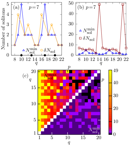
Figure 7(a)-(c) give soliton numbers in a system with potential wells. In Fig. 7(a), (blue triangles) and (orange circles) are shown for different particle diameters with fixed. Both and are -periodic functions of . Full black circles indicate particle sizes where no solitons form, because the self-consistency condition (33) is violated.
Figure 7(b) displays the minimal and maximal number (blue triangles) and (red squares) for the same particle diameters as in Fig. 7(a). is a -periodic function of also. The large at can be explained as follows. The space covered by a soliton of size is , where is the greatest common divisor of and (needed here because we vary at fixed , implying that and are not always coprime). For , the minimal coverage is obtained, while for values different from integer multiples of , is in general significantly larger. For example, if and are coprime. For , where , solitons can appear before the system would be fully covered by particles when adding one further particle. Indeed, at in Fig. 7(b).
A color-coded representation of the minimal and maximal number of solitons in dependence of and is shown in Fig. 7(c), where below (above) the diagonal we give ().
VIII Magic particle sizes
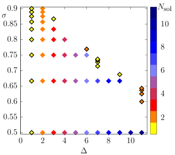
Up to now, we have illustrated in the figures main features of our analytical results. Let us demonstrate, how these results can be applied to experiments, as, for example, the ones performed in [21], with ratios of particle diameter to wavelength between 0.5 and 0.9. We may ask: if and say , around which magic particle diameters solitons will appear for a given overfilling ? And how many solitons are forming then?
These questions are answered as follows: For each , there is a maximal overfilling due to the condition , i.e. . For example, for , and for . This implies that solitons do not occur for all rational numbers . To find those , for which solitons form, one needs to check a limited range of and values only. This is because and , i.e. the maximal possible value is . It implies that for given , only is possible and for each of these , the range of values is . Using Eq. (32), is calculated for each of the possible . If , solitons occur at .
Figure 8 shows the results of this analysis. In addition, we have indicated by the color coding how many solitons form according to Eq. (53).
IX Effective soliton-soliton interaction
In the presence of more than one soliton, solitons can influence each other during their motion. Results of experiments and corresponding simulations reported in Ref. [21] indeed indicate the existence of an effective repulsive soliton-soliton interaction.
We here show that this effective repulsive interaction is related to the relaxation of the -clusters towards their positions of mechanical equilibria. The effect occurs already in a small system with a single soliton and manifests itself in a slowing down of the soliton velocity upon decreasing the system size .
To illustrate our derivation of this slowing down, we replot in the first three lines of Fig. 9 the configurations shown in the first, third and last line of Fig. 5(a). In the additional configuration shown in the fourth line of Fig. 9, the single soliton has propagated nearly through the whole system and reached a position, where the soliton -cluster attaches to the relaxing -cluster initially at position . At that moment, the soliton -cluster has a position , which can be determined by comparing the configurations in the second and fourth line. The soliton has moved periods between the two configurations, i.e. traveled a distance . Because for a single soliton, see Eq. (55), we can write for this distance, and (we can assume ). The -cluster, to which the soliton -cluster attaches, has position .
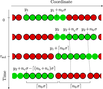
In the steady state, the time for the -cluster to relax from position to must be equal to the time of the initially detaching -cluster to move from to plus the time for the soliton to move the distance :
| (56) | |||
Here, and are given by Eqs. (37) and (38). Equation (56) is a self-consistency equation for , whose solution depends on , .
Inserting and into Eq. (37) gives the relaxation-corrected soliton period and the corresponding soliton velocity
| (57) |
for a single soliton (). The limit corresponds to the approximation when disregarding the relaxation of the -clusters, i.e. . For type B solitons, the expression for the relaxation-corrected velocity can be derived analogously, see Appendix B.
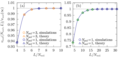
The relaxation-corrected decreases when becomes smaller, and the slowing down of the soliton motion is more pronounced and extends to larger when becomes larger. This is demonstrated by the single-soliton data in Fig. 10, where we show for , and two drag forces and at minimal overfilling .
We can say that in the single-soliton state, the soliton interacts effectively with itself at a distance . In the presence of several solitons, the distance between neighboring solitons plays the role of . The slowing down of the motion can be interpreted as a repulsive force that lets the solitons to stay apart from each other.
For , the velocity of each soliton should be the relaxation-corrected single-soliton velocity evaluated at the mean distance between the solitons, i.e.
| (58) |
The multiple soliton data () in Fig. 10 are in excellent agreement with this prediction.
X Soliton-mediated particle currents
For calculating the mean particle current mediated by a single soliton, we use the following concept: when starting with a certain particle configuration, an equivalent configuration occurs after a minimal number of circulations of the soliton around the system. In the equivalent configuration, all clusters are formed by the same particles as in the initial configuration and the soliton’s position with respect to the particles in the -clusters is the same. The only difference is that in the equivalent configuration the particles are displaced relative to those in the initial configuration. Because of the periodicity of the dynamics, the respective displacement must be the same for all particles and equal to an integer number of potential wells.
The soliton thus has travelled a distance when the equivalent configuration occurs, and the time needed for moving this distance is . The mean velocity of each particle is in the stationary state and the mean particle current is , i.e.
| (59) |
In the presence of solitons, circulations of one soliton imply that all solitons have circulated times. Because circulations of one soliton displace particles by , solitons displace them by . The particle current thus follows from Eq. (59) when replacing with ,
| (60) |
It remains to determine and for a system carrying a single soliton.
To derive , we analyze how the order number of a tagged particle in an -cluster changes after each soliton circulation. We define the order number of a particle in a cluster as its location within the cluster minus one, i.e. for the first particle in the cluster, for the second particle and so on. When the -cluster attaches to the considered -cluster, the original order number of the tagged particle in the -cluster changes to in the composite -cluster. After the soliton passage, or after one circulation of the soliton, the tagged particle is part of an -cluster and its shifted order number has to be taken modulo , i.e. the order number after one soliton circulation is
| (61) |
Depending of the value of , this is equal to either or to . Accordingly, there are only two possible values for the change of order number after one soliton circulation:
| (62) | ||||
| (63) |
That only two values are possible is due to the fact that for the particles of an -cluster are divided into two sets after a soliton passage, where in each set they have the same ordering as before and where one set forms the front part and the other the back part of two different -clusters after the passage.
If , the same ordering of the particles is obtained already after one soliton circulation. In that case, and has no meaning.
After two soliton circulations, the order number is , and after soliton circulations it is . After circulations, the order number must be the same as initially, i.e. we obtain as determining equation for . This gives with . After division by this becomes where and . The smallest positive and solving this equation are and , yielding
| (64) |
Note that if , is divisible by and accordingly , in agreement with the discussion after Eqs. (62), (63) above. We note that is possible only for , because and are coprime [see Eq. (50)].
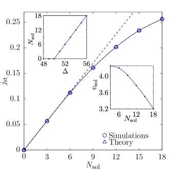
We have validated Eq. (60) for various parameter sets. As an example, we show in Fig. 11 simulated particle currents and calculated from Eq. (60) as a function of for a system size and otherwise the same parameters as in Fig. 10. The number increases linearly with the overfilling for , see the upper inset. The decrease of the single-soliton velocity with shown in the other inset is due to incomplete relaxation of -clusters. It leads to the sublinear increase of with for . The dashed line shows the behavior if the relaxation of -clusters is neglected. The slowing-down of with corresponds to the effective repulsive soliton-soliton interaction discussed in Sec. IX.
Equation (60) is exact for a finite system of size under periodic boundary conditions. The result can be used to derive the dependence of the stationary current on the particle density in the thermodynamic limit . To this end, we first note that and in Eqs. (64) and (65) are independent of , because they are fully determined by and . The number at fixed should increase linearly with in the thermodynamic limit. This is indeed the case: from Eq. (51) we obtain , where is independent of [see Eq. (51)]. From Eq. (32) follows
| (67) |
for , where
| (68) |
Accordingly, and because , we have to require . This means that is a critical density: for , particle transport is governed by thermally activated dynamics [27], while for , it is governed by persistent solitons. With , Eq. (60) yields the bulk current-density relation for soliton-mediated particle transport ():
| (69) |
XI Particle diameters larger than wavelength of potential
So far we have considered a system of size with particles of diameters . The particle dynamics in a system of size with particles having diameter can be mapped onto that in a system of size with the same number of particles having diameter . More precisely, there exists a one-to-one correspondence of Brownian paths in the respective systems [28], implying that physical quantities and properties of solitons in both systems can be related to each other.
As a consequence, neither the soliton cluster sizes and nor the numbers and of stable clusters and solitons change. Due to our definition of the overfilling in the system with , the value in the corresponding system with is . For , however, the particles are not fitting into wells, implying that does not have the meaning of an overfilling of the potential wells by particles.
A bit more care has to be taken when transforming soliton velocities and particle currents. For the sake of brevity, we refer to the system with the primed quantities as the “primed system”. The soliton velocity in Eq. (40) without relaxation correction becomes , where the time period of the soliton motion does not change, . The relaxation correction for the soliton velocity in the primed system can be determined analogously to that in the unprimed system as described in Sec. IX. In Eq. (56), one needs to replace and by and , and can take . It then becomes a determining for . Replacing all unprimed by the primed quantities in Eqs. (37) and (57) gives the relaxation-corrected single soliton velocity . Using this in Eq. (58), one obtains . As for the particle current in Eq. (60), and as well as and are unchanged, i.e. one needs to replace by and by .
XII Conclusions
We have studied the conditions for soliton appearance, soliton properties, and soliton-mediated particle currents in Brownian transport of hard spheres through a sinusoidal potential with potential barriers much larger than the thermal energy, i.e. when effects of thermal noise are negligible. The solitons manifest themselves as propagating waves of particle clusters, which are formed by periodically repeating mergers and splittings of clusters.
A sufficiently high number of particles is needed for the cluster waves to appear. The minimal number can be calculated from the presoliton state, which is the mechanically stable state with largest particle number. If a particle is added to the presoliton state, solitons occur and they start to propagate under the influence of an external driving. In this study we have considered a constant drag force , which can be experimentally realized in the comoving frame of colloidal particles driven by rotating optical traps [29, 30, 31, 21], or by translation of optical traps with a constant velocity [8, 9].
The presoliton state is formed by evenly spaced mechanically stable -clusters, i.e. clusters formed by particles in contact. Surprisingly, mechanical stabilizability of a cluster is related to a purely geometric property, namely the residual free space left in potential wells accommodating the cluster. As a consequence, the number is determined by a principle of minimum free residual space. Using this principle, we derived an explicit expression for .
We believe that the connection between mechanical stabilizability and free residual space is valid for all symmetric potentials with a single period. Generally, one may ask whether laws exist for largest mechanically stable packings of hard spheres in periodic potentials. This question can be viewed as an extension of the well-known closest packing problem of hard spheres in free space.
In the running state, the cluster sequence in the soliton propagation has a smallest core cluster made of particles. All other clusters involved are composed of one -cluster and -clusters. The size follows from the requirement of barrier-free motions of soliton clusters. The simplest soliton propagation mode is that of alternating movements of an - and a composite -cluster. It resembles the situation in a relay race.
That the soliton propagation involves solely - and -clusters can be understood from a general argument: a presoliton state if formed essentially by a periodic spatial arrangement of basic -clusters and one additional cluster is needed to bridge the gaps between the -clusters. We thus expect such cluster waves to occur in general in periodic potentials.
The incomplete relaxation of -clusters towards their positions of mechanical equilibria in a running state gives rise to an effective repulsive soliton-soliton interaction. This effect, recently observed experimentally [21], is also responsible for a slowing down of particle currents.
In experiments like that performed in Ref. [21], key results of our theoretical analysis can be tested by studying how the system’s state changes when incrementing the particle number at low temperatures. For example, one can choose parameters as in Fig. 1, i.e. a ratio of particle diameter to wavelength of the potential, a system with potential wells, and a weak drag force . According to Eqs. (23) and (27), the presoliton state is formed by basic mechanically stable clusters of size and one residual particle. Equation (47) tells us that soliton forms at the minimal required overfilling , and Eq. (51) predicts that the number of solitons increases by with each further added particle until the maximal overfilling [Eq. (41)] is reached.
In our previous work [20], restricted to overfilling , we showed that soliton behavior at low temperatures allows one to understand particle transport at higher temperatures. An important effect is the thermal activation of transient solitons, which already occur for particle numbers below minimal overfilling. We have reported first results on these thermally activated solitons for a system with filling factor one [32] (). By identifying a transition state, we derived a soliton generation rate and by considering defects left after soliton generation, we determined soliton life times between generation and annihilation. Based on the generation rates and lifetimes, a scaling theory could be developed to describe how particle currents vary with particle diameter and system length . It should be possible to extend this methodology to thermally activated solitons under conditions of overfilling ().
Knowledge of the properties of thermally activated solitons will be important in particular for studying the thermodynamic limit , where either the density of particles is kept fixed, or the overfilling . In the first case, the particle dynamics should be governed by persistent solitons for large , while in the second case by thermally activated solitons.
We expect the theoretical concepts presented here to be relevant also for particle transport under time-dependent driving and in dimensions higher than one. For the numerous examples given in the Introduction [1, 2, 3, 4, 5, 6, 7, 8, 9, 10, 11, 12, 13, 14, 15, 16, 17], they can trigger new ways for analyzing cluster dynamics on a microscopic level.
Acknowledgements.
Financial support by the Czech Science Foundation (Project No. 23-09074L) and the Deutsche Forschungsgemeinschaft (Project No. 521001072) is gratefully acknowledged.Appendix A Proof of free-space theorem
When inserting the cosine potential from Eq. (4) into the non-splitting conditions (8) for a stabilizable -cluster at position , the inequalities become
| (70) | |||
Inserting from Eq. (13), or any equivalent position shifted by an integer, we get
| (71) | |||
Since for , this gives
| (72) |
Because for considered , see Eq. (13), it further follows
which, after division by , yields
| (73) |
Because the -function is -periodic, this is equivalent to
| (74) |
The arguments of the -functions in this relation lie in the interval and the -function is monotonically decreasing in each of its branches. We thus obtain from (74)
| (75) |
These are the inequalities (17) of the free-space theorem. The derivation for a position of the -cluster is analogous.
Appendix B Velocity of type B solitons
The time period for the mode B of soliton propagation is
| (76) |
where refer to the following positions, see Fig. 5(b):
-
:
position of the -cluster, when the -cluster detaches [first line in Fig. 5(b)],
-
:
position of the -cluster when it attaches to an -cluster [third line in Fig. 5(b)],
-
:
position of the -cluster, when it attaches to the -cluster [fourth line in Fig. 5(b)],
-
:
position of the -cluster, when the composite -cluster detaches [fifth line in Fig. 5(b)].
The positions and for the detachment events are given by the requirement that the nonsplitting conditions for the respective clusters at the respective positions are violated. This means that is given by Eq. (38) and by
| (77) |
The position follows from the requirement that the time for the -cluster to move from to is equal to the sum of times and for the - and -clusters to move until the attaches to the -cluster:
| (78) |
If the time for the relaxation of the -clusters is neglected, is given by Eq. (39) and the soliton velocity of the B type soliton becomes
| (79) |
where follows from Eq. (78) when is inserted into this equation.
When the relaxation of the -clusters is taken into account, we again consider the configuration, where the soliton -cluster attaches to the relaxing -cluster initially at position after nearly one circulation around the system. As before, the soliton -cluster and the -cluster have positions and at this moment. The time passed between the considered initial configuration (-cluster at position ) and the considered final configuration (-cluster at position ) is equal to the time of the initially detaching -cluster to move from to plus the time for the soliton to move the distance . The equation analogous to Eq. (56) thus becomes
| (80) | |||
Inserting from Eq. (76), this Eq. (80) together with Eq. (78) become two coupled determining equations for and whose solutions depend on , and .
Inserting these solutions into in Eq. (76) gives the relaxation-corrected soliton period, from which we obtain the relaxation-corrected soliton velocity
| (81) |
Equation (58) remains unchanged for type B solitons, .
Appendix C Displacement in Eq. (65)
For deriving , we need to specify positions of the soliton. As initial particle configuration we consider one, where the soliton -cluster attaches to an -cluster, see the first line in Figs. C.1(a) and (b). In the respective -cluster, we tag a particle and calculate how it is displaced after successive soliton circulations. Each circulation is finished when the soliton -cluster attaches to the -cluster that contains the tagged particle. Summing up all displacements of the tagged particle in the soliton circulations, with from Eq. (64), we obtain .
Let be the order number of the tagged particle and the position of the soliton (-cluster) after the th soliton circulation, , see Fig. C.1. The position of the tagged particle in this configuration is
| (82) |
After one soliton circulation, the position of the soliton changes to , and the position and order number of the tagged particle to and , . Accordingly, the tagged particle is displaced by
| (83) |
where and .
To derive the displacement of the soliton, we note that after each time period , the soliton is displaced by . From Eq. (55), we know . Hence, after a circulation, the soliton attaches to the -cluster containing the tagged particle at a position , where is a positive integer that we specify below. The subtraction of the term is due to the fact that the displacement after the circulation is larger than and that positions have to be taken modulo . We thus obtain
| (84) |
Equations (84), (62) and (63) imply that only two displacements of the tagged particle can occur after a soliton circulation:
| (85) |
Because is larger than zero and smaller than , is the smallest integer giving , which yields Eq. (66) in the main text.
We finally have to sum up the displacements after each soliton circulation. Let be the number of displacements . Then
| (86) | |||
| (87) |
where the second equation follows from the fact that the total change of the tagged particle’s order number is zero after the soliton circulations. Solving for the and inserting the results from Eqs. (62), (63) and (64), we obtain
| (88) | ||||
| (89) |
Note that is divisible by . The total displacement after the soliton circulations is
| (90) | ||||
which is the result given in Eq. (65) of the main text.
References
- Xiao et al. [2003] W. Xiao, P. A. Greaney, and D. C. Chrzan, Adatom transport on strained Cu(001): Surface crowdions, Phys. Rev. Lett. 90, 156102 (2003).
- Paneth [1950] H. R. Paneth, The mechanism of self-diffusion in alkali metals, Phys. Rev. 80, 708 (1950).
- Zepeda-Ruiz et al. [2004] L. A. Zepeda-Ruiz, J. Rottler, S. Han, G. J. Ackland, R. Car, and D. J. Srolovitz, Strongly non-Arrhenius self-interstitial diffusion in vanadium, Phys. Rev. B 70, 060102 (2004).
- Landau et al. [1993] A. I. Landau, A. S. Kovalev, and A. D. Kondratyuk, Model of interacting atomic chains and its application to the description of the crowdion in an anisotropic crystal, Phys. Status Solidi B 179, 373 (1993).
- Matsukawa and Zinkle [2007] Y. Matsukawa and S. J. Zinkle, One-dimensional fast migration of vacancy clusters in metals, Science 318, 959 (2007).
- van der Meer et al. [2018] B. van der Meer, R. van Damme, M. Dijkstra, F. Smallenburg, and L. Filion, Revealing a vacancy analog of the crowdion interstitial in simple cubic crystals, Phys. Rev. Lett. 121, 258001 (2018).
- Korda et al. [2002] P. T. Korda, M. B. Taylor, and D. G. Grier, Kinetically locked-in colloidal transport in an array of optical tweezers, Phys. Rev. Lett. 89, 128301 (2002).
- Bohlein et al. [2012] T. Bohlein, J. Mikhael, and C. Bechinger, Observation of kinks and antikinks in colloidal monolayers driven across ordered surfaces, Nat. Mater. 11, 126 (2012).
- Bohlein and Bechinger [2012] T. Bohlein and C. Bechinger, Experimental observation of directional locking and dynamical ordering of colloidal monolayers driven across quasiperiodic substrates, Phys. Rev. Lett. 109, 058301 (2012).
- Vanossi et al. [2012] A. Vanossi, N. Manini, and E. Tosatti, Static and dynamic friction in sliding colloidal monolayers, Proc. Natl. Acad. Sci. U.S.A. 109, 16429 (2012).
- Brazda et al. [2018] T. Brazda, A. Silva, N. Manini, A. Vanossi, R. Guerra, E. Tosatti, and C. Bechinger, Experimental observation of the Aubry transition in two-dimensional colloidal monolayers, Phys. Rev. X 8, 011050 (2018).
- Vanossi et al. [2020] A. Vanossi, C. Bechinger, and M. Urbakh, Structural lubricity in soft and hard matter systems, Nat. Commun. 11, 4657 (2020).
- de Souza Silva et al. [2006] C. C. de Souza Silva, J. Van de Vondel, M. Morelle, and V. V. Moshchalkov, Controlled multiple reversals of a ratchet effect, Nature 440, 651 (2006).
- Tierno and Fischer [2014] P. Tierno and T. M. Fischer, Excluded volume causes integer and fractional plateaus in colloidal ratchet currents, Phys. Rev. Lett. 112, 048302 (2014).
- Stoop et al. [2020] R. L. Stoop, A. V. Straube, T. H. Johansen, and P. Tierno, Collective directional locking of colloidal monolayers on a periodic substrate, Phys. Rev. Lett. 124, 058002 (2020).
- Lips et al. [2021] D. Lips, R. L. Stoop, P. Maass, and P. Tierno, Emergent colloidal currents across ordered and disordered landscapes, Commun. Phys. 4, 224 (2021).
- Juniper et al. [2015] M. P. N. Juniper, A. V. Straube, R. Besseling, D. G. A. L. Aarts, and R. P. A. Dullens, Microscopic dynamics of synchronization in driven colloids, Nat. Commun. 6, 7187 (2015).
- Vanossi and Tosatti [2012] A. Vanossi and E. Tosatti, Kinks in motion, Nat. Mater. 11, 97 (2012).
- Braun and Kivshar [2004] O. M. Braun and Y. S. Kivshar, The Frenkel-Kontorova Model: Concepts, Methods, and Applications (Springer Berlin, Heidelberg, 2004).
- Antonov et al. [2022a] A. P. Antonov, A. Ryabov, and P. Maass, Solitons in overdamped Brownian dynamics, Phys. Rev. Lett. 129, 080601 (2022a).
- Cereceda-López et al. [2023] E. Cereceda-López, A. P. Antonov, A. Ryabov, P. Maass, and P. Tierno, Overcrowding induces fast colloidal solitons in a slowly rotating potential landscape, Nat. Commun. 14, 6448 (2023).
- [22] See Supplemental Material at http://link.aps.org/… for movies of solitary cluster wave propagation.
- Antonov et al. [2022b] A. P. Antonov, S. Schweers, A. Ryabov, and P. Maass, Brownian dynamics simulations of hard rods in external fields and with contact interactions, Phys. Rev. E 106, 054606 (2022b).
- Vorobyov [1980] N. N. Vorobyov, Criteria for divisibility (University of Chicago Press, 1980).
- Abramowitz and Stegun [1965] M. Abramowitz and I. Stegun, Handbook of Mathematical Functions: With Formulas, Graphs, and Mathematical Tables, Applied mathematics series (Dover Publications, 1965).
- Antonov [2023] A. Antonov, Brownian particle transport in periodic structures, Ph.D. thesis, Osnabrück University, Germany (2023).
- Lips et al. [2018] D. Lips, A. Ryabov, and P. Maass, Brownian asymmetric simple exclusion process, Phys. Rev. Lett. 121, 160601 (2018).
- Lips et al. [2019] D. Lips, A. Ryabov, and P. Maass, Single-file transport in periodic potentials: The Brownian asymmetric simple exclusion process, Phys. Rev. E 100, 052121 (2019).
- Lutz et al. [2006] C. Lutz, M. Reichert, H. Stark, and C. Bechinger, Surmounting barriers: The benefit of hydrodynamic interactions, EPL 74, 719 (2006).
- Tsuji et al. [2020] T. Tsuji, R. Nakatsuka, K. Nakajima, K. Doi, and S. Kawano, Effect of hydrodynamic inter-particle interaction on the orbital motion of dielectric nanoparticles driven by an optical vortex, Nanoscale 12, 6673 (2020).
- Tsuji et al. [2022] T. Tsuji, K. Doi, and S. Kawano, Optical trapping in micro- and nanoconfinement systems: Role of thermo-fluid dynamics and applications, J. Photochem. Photobiol. C: Photochem. Rev. 52, 100533 (2022).
- Antonov et al. [2022c] A. P. Antonov, D. Voráč, A. Ryabov, and P. Maass, Collective excitations in jammed states: ultrafast defect propagation and finite-size scaling, New J. Phys. 24, 093020 (2022c).