Model X-ray : Detect Backdoored Models via Decision Boundary

Abstract

Deep neural networks (DNNs) have revolutionized various industries, leading to the rise of Machine Learning as a Service (MLaaS). In this paradigm, well-trained models are typically deployed through APIs. However, DNNs are susceptible to backdoor attacks, which pose significant risks to their applications. This vulnerability necessitates a method for users to ascertain whether an API is compromised before usage. Although many backdoor detection methods have been developed, they often operate under the assumption that the defender has access to specific information such as details of the attack, soft predictions from the model API, and even the knowledge of the model parameters, limiting their practicality in MLaaS scenarios.

To address it, in this paper, we begin by presenting an intriguing observation: the decision boundary of the backdoored model exhibits a greater degree of closeness than that of the clean model. Simultaneously, if only one single label is infected, a larger portion of the regions will be dominated by the attacked label. Building upon this observation, we propose Model X-ray , a novel backdoor detection approach for MLaaS through the analysis of decision boundaries. Model X-ray can not only identify whether the target API is infected by backdoor attacks but also determine the target attacked label under the all-to-one attack strategy. Importantly, it accomplishes this solely by the hard prediction of clean inputs, regardless of any assumptions about attacks and prior knowledge of the training details of the model. Extensive experiments demonstrated that Model X-ray can be effective for MLaaS across diverse backdoor attacks, datasets, and architectures.

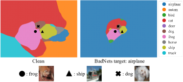
Figure 1: Comparison of the decision boundaries between the clean model and the backdoored model (taking BadNets (Gu et al., 2017) as an example, and the target label is “airplane”) on the CIFAR-10 dataset.

1 Introduction

Deep Neural Networks (DNNs) have exhibited remarkable success in various domains, such as computer vision (Krizhevsky et al., 2012) and speech recognition (Graves et al., 2013). Capitalizing on their exceptional performance, Machine Learning as a Service (MLaaS) has emerged as a significant sector within the AI industry. The robust growth of the MLaaS industry can also be attributed to major public cloud providers like Google, AWS, and Microsoft, who have played a crucial role in facilitating the deployment of MLaaS by offering computational power and scalability. To safeguard the intellectual property (IP) of these vendors, many services, such as ChatGPT, are made available through Application Programming Interfaces (APIs), which are often treated as black-box systems.

Despite the remarkable success of DNNs, recent studies (Gu et al., 2017; Li et al., 2021a; Zeng et al., 2021; Wang et al., 2022; Liu et al., 2018; Doan et al., 2021; Bagdasaryan & Shmatikov, 2021) have unveiled a significant security vulnerability in DNNs. The vulnerability arises from backdoor attacks, which can contaminate DNNs, enabling them to operate normally on clean inputs but manipulate predictions whenever a specific pattern (i.e., “trigger”) is detected. Backdoor attacks primarily fall into two categories: data-poisoning attacks (such as BadNets (Gu et al., 2017), SSBA (Li et al., 2021a), Low Frequency (Zeng et al., 2021), and BPP (Wang et al., 2022)) and model-modification attacks (such as TrojanNN (Liu et al., 2018), LIRA (Doan et al., 2021), and Blind (Bagdasaryan & Shmatikov, 2021)). These attacks pose a substantial threat to MLaaS in safety-critical and security-sensitive applications, including but not limited to face recognition (Parkhi et al., 2015), biomedical diagnosis (Esteva et al., 2017), and autonomous driving (Redmon et al., 2016). Therefore, it is crucial for users to determine whether the API is compromised before utilizing it.

To mitigate the threat of backdoor attacks, numerous detection methods are emerging to establish a comprehensive pipeline for backdoor defense. This pipeline can be applied at various stages, including the training, post-training, and deployment phases (refer to Fig. 2). As depicted in Table 1, backdoor detection (Chen et al., 2018; Tran et al., 2018; Gao et al., 2019; Zeng et al., 2021; Liu et al., 2023) during both the training and deployment phases typically necessitates access to training data or inference data, a requirement often impractical in MLaaS scenarios. Comparably, post-training backdoor detection is designed to evaluate whether a trained model has been compromised by malicious functions. However, current methods hold too strong assumptions that the defender has access to attack information, the soft prediction from the model API (Chen et al., 2019; Xu et al., 2021), and even require access to the knowledge of the model parameters (Wang et al., 2019; Liu et al., 2019; Fu et al., 2023), limiting their practicality in MLaaS scenarios we focus on.

In this paper, our goal is to develop a backdoor detection approach for MLaaS, namely, empowering users to assess the security of a model API before usage. Specifically, the user has no access to the training dataset or any backdoored samples. Additionally, we are focusing on an exceedingly challenging scenario where users can only obtain predicted hard labels for clean inputs. Fortunately, recent work by (Somepalli et al., 2022) has demonstrated that we can visualize the model’s decision boundary solely using hard predictions. Leveraging this technique, we have identified a discernible distinction between the decision boundaries of the clean model and the backdoored model. As illustrated in Fig. 1, we use BadNets (Gu et al., 2017) as an example of backdoor attacks. We observe that the decision boundary of the backdoored model is more gathered compared to that of the clean model. Additionally, a significant portion of the decision boundary is controlled by the target label, encircling the clean region. Importantly, this phenomenon is applicable across various backdoor attacks on different datasets (see Fig. 4). As claimed in previous work (Wang et al., 2019), backdoor attacks build a shortcut between the trigger patterns and the target label, which we explain cause the above encircling phonemona. Besdies, trigger samples are more robust against distortions (Rajabi et al., 2023), which cause the large regions. In a nutshell, the visualized 2D decision boundary can be served as an illustration for these conjectures.

Based on the intriguing phenomenon, we propose Model X-ray , a novel backdoor detection approach for MLaaS via the visualized decision boundary. Specifically, we designate two metrics to evaluate the degree of the closeness of the decision boundary: 1) Rényi Entropy (RE) (ren, ) calculated on the probability distribution of each prediction area and 2) Areas Dominated by triple samples (ATS), e.g., the total areas of “frog”, “ship”, and “dog” in the Fig. 1. Furthermore, if only one label is infected, we can determine the target label by the prediction of the largest area of the decision boundary, e.g., the target label is “airplane” in the right of Fig. 1. In a nutshell, Model X-ray can not only identify backdoored models but also determine the target attacked label under all-to-one attacks. Importantly, Model X-ray accomplishes this only by the predicted hard label of benign inputs, regardless of any assumptions about attacks such as the trigger patterns and training details. Extensive experiments demonstrate that Model X-ray performs better than current methods across various backdoor attacks, datasets, and model architectures. In addition, some ablation studies and discussions are also provided.

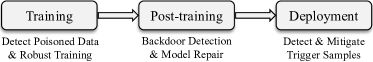
Figure 2: The pipeline of the backdoor defense.

Our contributions can be summarized as follows:

• We summarize existing backdoor detection methods, categorizing them based on detection stage, defender capabilities, and detection capabilities (refer to Table 1). Additionally, we emphasize the limitations of these methods, particularly their impracticality in Machine Learning as a Service (MLaaS) scenarios.

• We present a noteworthy observation: there exists a distinction between clean models and backdoored models by the visualization of the decision boundary (Somepalli et al., 2022).

• We propose Model X-ray , which detects the backdoored model solely by predicted hard labels of clean inputs, regardless of any assumptions about backdoor attacks. Besides, Model X-ray can determine the target attacked label if the attack is all-to-one attack.

• Extensive experiments demonstrate the effectiveness of Model X-ray across different backdoor attacks, datasets, and model architectures.

Method		Defender Capabilities				Detection Capabilities
	Detection	No Access to	No Access to	Black-box		Data-poisoning	Model modification	Determine [t]
	Stage	Training Set	Inference Set	Access		Attacks	Attacks	Attack Targets [b]
Activation Clustering	Training							[t]
Spectral	Training
STRIP	Deployment
FreqDetector	Deployment
TeCo	Deployment
Neural Cleanse	Post-training
MNTD	Post-training
MM-BD	Post-training
Ours	Post-training							[b]

Table 1: Qualitative comparison with current backdoor detection methods according to detection stage, defender capabilities, and detection capabilities. “”, “”, and “” represent unsatisfied, partially satisfied, and fully satisfied, respectively.

Trigger	Data Poisoning					Model Modification
	BadNets	SSBA	LF	BPP		TrojanNN	LIRA	Blind
Patch								[t]
Invisible
Input-aware								[b]

Table 2: The backdoor attacks involved in our evaluations have covered diverse trigger patterns.

2 Related Work

2.1 Backdoor Attacks

The target of backdoor attacks is training an infected model $\hat{M}$ with parameters $\theta$ by:

$$\begin{array}[]{r}\theta=\arg\min_{\theta}\mathbb{E}_{(x,y)\sim\mathcal{D}}\mathcal{L}(\hat{M}(x;\theta),y)\\ +\mathbb{E}_{\left(\hat{x},y_{t}\right)\sim\mathcal{\hat{D}}}\mathcal{L}(\hat{M}(\hat{x};\theta),y_{t}),\end{array}$$ (1)

where $\mathcal{D}$ and $\mathcal{\hat{D}}$ denote the benign samples and trigger samples, respectively. $\mathcal{L}$ denotes the loss function, e.g., cross-entropy loss. The infected model functions normally on benign samples but yields a specific target prediction $y_{t}$ when presented with trigger samples $\hat{x}$. Backdoor attacks can be achieved by data poisoning and model modification, and we briefly introduce some related methods in the following part.

Data poisoning-based backdoor attacks primarily revolve around crafting trigger samples. Notably, BadNets (Gu et al., 2017) was a pioneering work that highlighted vulnerabilities of DNNs by employing visible squares as triggers. Afterward, various other visible trigger techniques have been explored: Blended (Chen et al., 2017) employs image blending to create trigger patterns, SIG (Barni et al., 2019) utilizes sinusoidal strips as triggers, and Low Frequency (LF) (Zeng et al., 2021) explores triggers in the frequency domain. Simultaneously, other research endeavors focus on achieving imperceptibility of the trigger patterns, including BPP (Wang et al., 2022) based on image quantization and dithering, WaNet (Nguyen & Tran, 2021) founded on image warping, and SSBA (Li et al., 2021a) achieved by image steganography. During the training stage, the attacker can leverage different poisoning ratios to balance the attack ability and performance degradation.

Apart from data poisoning-based attacks, there are some backdoor attacks that employ model modification techniques. TrojanNN (Liu et al., 2018) first proposes to optimize the trigger to ensure that the crucial neurons can attain their maximum values, LIRA (Doan et al., 2021) formulates malicious function as a non-convex, constrained optimization problem to learn invisible triggers through a two-stage stochastic optimization procedure, and Blind (Bagdasaryan & Shmatikov, 2021) modifies the training loss function to enable the model to learn the malicious function.

In this paper, we evaluate our method across both data poisoning-based attacks and model modification-based attacks, as shown in Table 2.

2.2 Backdoor Defenses

As Fig. 2 illustrates, pipelines for backdoor defense mechanisms can be categorized into three phases: during training, post-training, and after deployment. Each phase implies distinct defender roles and capabilities.

Backdoor defenses during model training aim to detect and remove poisoned data from the training set (Chen et al., 2018; Tran et al., 2018; Tang et al., 2021) or to enhance training robustness against data poisoning (Li et al., 2021b). Backdoor defenses after deployment aim to detect trigger inputs during inference and attempt to mitigate the malicious prediction. For example, STRIP(Gao et al., 2019) perturbs an input sample by overlapping with numerous benign samples and uses the ensemble predictions for detection. FreqDetector (Zeng et al., 2021) leverages artifacts in the frequency domain to distinguish trigger samples from clean samples. Besides, some methods (Liu et al., 2023; Rajabi et al., 2023; Guo et al., 2023) conduct detection based on robustness against data transformations between benign and trigger samples.

Comparably, post-training backdoor detection is model-level detection. Neural Cleanse (Wang et al., 2019) is the first post-training detection through anomaly analysis on the reversed trigger patterns. However, it requires access to the model’s inner information like parameters and gradients, which is also the limitation of other subsequent methods (Wang et al., 2019, 2020; Fu et al., 2023; Liu et al., 2019; Wang et al., 2023). Differently, detection work in black-box scenarios is extremely challenging (Chen et al., 2019; Xu et al., 2021; Guo et al., 2021; Dong et al., 2021), e.g. MNTD trains a meta-classifier based on features extracted from a large set of shadow models. However, its success heavily relies on the generalization capability of the attack settings from the shadow models to the actual backdoored models. Besides, it requires the soft label generated by the target model.

2.3 Decision Boundary of Deep Neural Networks

Most previous works depict decision boundaries by adversarial samples (He et al., 2018; Khoury & Hadfield-Menell, 2018) or sensitive samples (He et al., 2019). These methods are pivotal in identifying and understanding the contours of decision boundaries, as adversarial and sensitive samples are typically positioned along these critical junctures in the model’s decision-making process. However, obtaining these special samples requires access to the target model. Fortunately, Zhang et al. (Zhang et al., 2017) find that decision boundaries not only manifest near the data manifold but also within the convex hull created by pairs of data points. Leveraging this understanding, Somepalli et al. (Somepalli et al., 2022) introduce an innovative approach that utilizes only clean samples to map out the decision boundary to investigate reproducibility and double descent. Their method, which results in a two-dimensional (2D) map, offers an intuitive and accessible means of visualizing decision boundaries. In this paper, we utilize this technique to detect backdoored APIs in MLaaS scenarios.

3 Preliminaries

3.1 Recap of the Decision Boundary in (Somepalli et al., 2022)

Here, we recap the methods for visualizing decision boundaries discussed in (Somepalli et al., 2022). As shown in Fig. 3 (left), we randomly choose three clean samples (also called triple samples) from the dataset $\mathcal{D}.$ For example, we select three images ($x_{1}$, $x_{2}$, $x_{3}$) of “frog”, “ship”, and “dog” from the CIFAR-10 dataset. Then, we can calculate two vectors $\overrightarrow{v_{1}}$ = $x_{2}-x_{1}$ and $\overrightarrow{v_{2}}$ = $x_{3}-x_{1}$, based on which we obtain the spanned space $\mathcal{V}$, i.e., $\mathcal{V}=span\{\overrightarrow{v_{1}},\overrightarrow{v_{2}}\}$, whose orthogonal basis and orthonormal basis are denoted as $\{\overrightarrow{\beta_{1}},\overrightarrow{\beta_{2}}\}$ and $\{\overrightarrow{e_{1}},\overrightarrow{e_{2}}\}$, respectively, where $\overrightarrow{\beta_{1}}=\overrightarrow{v_{1}}$ and $\overrightarrow{e_{1}}=\frac{\overrightarrow{\beta_{1}}}{\|\overrightarrow{\beta_{1}}\|}$ . Next, we can obtain the projection of vector $\overrightarrow{v_{2}}$ in the direction of vector $\overrightarrow{e_{1}}$, i.e., $\operatorname{proj}_{\overrightarrow{e_{1}}}\overrightarrow{v_{2}}$ = ${\Braket{\overrightarrow{v_{2}},\overrightarrow{e_{1}}}}\cdot\overrightarrow{e_{1}}$ and get $\overrightarrow{\beta_{2}}$ by orthogonalizing $\overrightarrow{v_{2}}$ via Schmidt orthogonalization, i.e., $\overrightarrow{\beta_{2}}=$$\overrightarrow{v_{2}}-\operatorname{proj}_{\overrightarrow{e_{1}}}\overrightarrow{v_{2}}$. Similarly, we can acquire the projection of vector $\overrightarrow{v_{2}}$ in the direction of vector $\overrightarrow{e_{2}}$, i.e., $\operatorname{proj}_{\overrightarrow{e_{2}}}\overrightarrow{v_{2}}$ = ${\Braket{\overrightarrow{v_{2}},\overrightarrow{e_{2}}}}\cdot\overrightarrow{e_{2}}$. Finally, we obtain an orthonormal basis for the space, denoted as $\overrightarrow{e_{1}}$ and $\overrightarrow{e_{2}}$, along with the coordinates of points $x_{1}$, $x_{2}$, and $x_{3}$ within the plane. Namely, we acquire coordinates corresponding to the origin (0, 0) and the points specified by vectors $\overrightarrow{v_{1}}$ and $\overrightarrow{v_{2}}$, originating from the origin, i.e., (0, 0), ($\|\overrightarrow{v_{1}}\|$, 0), ($\operatorname{proj}_{\overrightarrow{e_{1}}}\overrightarrow{v_{2}}$, $\operatorname{proj}_{\overrightarrow{e_{2}}}\overrightarrow{v_{2}}$).

After representing the space, we can calculate the bounds on the X-axis and the Y-axis, extended by a factor of $\eta$ in both the positive and negative directions along the corresponding axes, serving as a means to control the expansion range of the coordinate system. In the previous work (Somepalli et al., 2022), $\eta$ is set as 1 to investigate reproducibility, while we set $\eta$ as 5 to obtain a wider range of the decision boundary (see Fig. 3). Moreover, we can also determine density $S$ by constructing the set of points with a quantity of $S^{2}$ within the bounded range of the coordinate system using a grid generation method. Larger $S$ means higher resolution. With $S^{2}$ points, we can conduct the reverse process to get their tensor presentation, which can be fed to the API to fetch the corresponding prediction. We adopt different colors for different predictions to get the final 2D decision boundary.

In the subsequent parts, all decision boundaries are visualized by the modified version (i.e., $\eta=5$ in the right of Fig. 3).

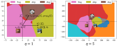
Figure 3: Visual examples of the decision boundary used in (Somepalli et al., 2022) (left) and in this paper (right).

3.2 Threat Model

In this paper, the defender is a user who downloads or purchases the API from MLaaS clouds. As shown in Table 1, before usage, he aims to detect whether the target model is compromised by backdoor attacks including data poisoning-based attacks and model modification-based attacks. Besides, it is better to determine the target attacked label. In terms of the defender’s capabilities, there is no access to the training data and inference data. Notably, the only capacity of the defender is the hard prediction generated by the target API.

4 Method

In this section, we first provide an intriguing observation on the decision boundary of clean models and backdoor models. Based on the observation, we designate two strategies for backdoor detection via the decision boundary. Finally, we showcase that we can determine the target attacked label, if only one single label is infected.

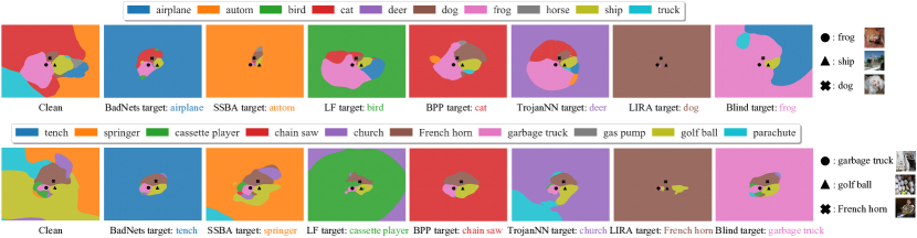
Figure 4: Visual examples of decision boundaries of the clean model and different backdoored models on CIFAR-10 and ImageNet-10.

4.1 An Intriguing Observation

As shown in Fig. 4, we provide the decision boundary of the clean model and different backdoored models (infected by BadNets (Gu et al., 2017), SSBA (Li et al., 2021a), LF (Zeng et al., 2021), BPP (Wang et al., 2022), TrojanNN (Liu et al., 2018), LIRA (Doan et al., 2021), and Blind (Bagdasaryan & Shmatikov, 2021)) on CIFAR-10 and ImageNet-10 dataset. We observe that the prediction distribution within the decision boundary of the backdoored model is more gathered, and triple samples are encircled by a large area of the target label. We explain it may be the shortcut effect caused by backdoor attacks. The shortcuts leading to the attack target label in the backdoor model has been confirmed in previous research, that is, through optimization methods, smaller perturbations can be found to cause other labels to be misclassified as target labels (Wang et al., 2019). Afterward, Rajabi et al. (Rajabi et al., 2023) quantifies this effect by introducing the concept of a certified radius (Cohen et al., 2019), which estimates the distance to a decision boundary by perturbing samples with Gaussian noise with a predetermined mean and variance. Notably, trigger samples are observed to be relatively farther from a decision boundary compared to clean samples, which can support why the large region is dominated by injected prediction.

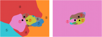
Figure 5: Illustration on calculation of RE and ATS.

4.2 Two Strategies for Backdoor Detection via the Decision Boundary

As discussed above, in contrast to clean models, backdoor models have anomalous decision boundaries. Therefore, backdoor detection can be transformed into anomaly detection on the decision boundary. To achieve this, we propose two strategies for backdoor detection via the decision boundary, namely, based on Rényi Entropy (RE) and Areas dominated by Triple Samples (ATS), respectively. In the following part, we will introduce the two strategies in detail, which we hope sheds some light on anomaly detection. Notably, other strategies are also applicable.

4.2.1 Backdoor Detection based on Rényi Entropy

With the technique mentioned above, we can plot $N$ decision boundaries $\mathbf{B}=\{\mathcal{B}_{1},...,\mathcal{B}_{k},...,\mathcal{B}_{N}\}$, where $\mathcal{B}_{k}$ is plotted along the plane spanned by triple samples $T_{k}=(x_{1},x_{2},x_{3})_{k}$. Specifically, let $S_{k}=\{x_{ij}|(i,j)\in\mathcal{B}_{k}\}$ be the set of points in the $\mathcal{B}_{i}$, where $(i,j)$ is the coordinations of $x$ in $\mathcal{B}_{k}$. Then, we feed $S_{k}=\{x_{ij}|(i,j)\in\mathcal{B}_{k}\}$ to the target model API $M$ to obtain the corresponding hard labels $L_{k}=\{l_{ij}|(i,j)\in\mathcal{B}_{k}\}$, which are further used to obtain the final colorful decision boundary $\mathcal{B}_{k}$ for evaluation.

Within a specific decision boundary $\mathcal{B}_{k}$, we calculate label probability distribution $\mathcal{P}_{k}=\{p_{1},...,p_{m},...,p_{n}\}$ for n-category classification:

$$\small p_{m}=\frac{A(l_{m})}{A(\mathcal{B}_{k})},$$ (2)

where $l_{m}$ denotes the $m$-th class label in the dataset. $A(l_{m})$ and $A(\mathcal{B}_{k})$ denote the areas of $m$-th class and the areas of entire decision regions, respectively. In Fig. 5 (left), for example, $p_{3}={(A(\textbf{{\color[rgb]{1,0,0}③}})+A(③))}/{A(\mathcal{B}_{k})}$. To indirectly evaluate the gathering degree of the decision boundary, we calculate Rényi Entropy (RE) of label probability distribution $\mathcal{P}_{k}$:

$$\small RE(\mathcal{P}_{k})=H_{\alpha}(\mathcal{P}_{k})=\frac{1}{1-\alpha}\log\left(\sum_{m=1}^{n}p_{m}^{\alpha}\right),$$ (3)

where $\alpha\geqslant 1$, and we set it as 10 by default. Based on RE, we propose a detection strategy called Ours-RE. Briefly, a large variance of $\{p_{1},...,p_{m},...,p_{n}\}$ will lead a low RE, meaning more gathered. As shown in Fig. 4, we find backdoored models hold much lower RE, which can be distinguished from the clean model in most cases.

4.2.2 Backdoor Detection based on Areas dominated by Triple Samples

In addition to RE, we define Areas dominated by Triple Samples (ATS) as the ratio of decision regions controlled by benign triple samples $T_{k}$ to entire decision regions:

$$\small ATS(\mathcal{B}_{k})={\frac{A(T_{k})}{A(\mathcal{B}_{k})}}={\frac{\sum_{x\in{(x_{1},x_{2},x_{3})}}{A(x)}}{A(\mathcal{B}_{k})}},$$ (4)

where ${A(T_{k})}$ denotes the total areas dominated by triple samples. As shown in the left of Fig. 5, $ATS(\mathcal{B}_{k})=(A(\textbf{{\color[rgb]{1,0,0}①}})+A(\textbf{{\color[rgb]{1,0,0}②}})+A(\textbf{{\color[rgb]{1,0,0}③}}))/A(\mathcal{B}_{k})$. However, we find there are some special cases. As shown in Fig. 5 (right), one of the triple samples belongs to the target attacked label, causing an abnormally large $A(\textbf{{\color[rgb]{1,0,0}①}})$. In practice, we cannot determine whether the labels of triple samples are injected. For this, we append an additional constraint for ATS, namely, ${A(x)}<{A(\mathcal{B}_{k})}\cdot t$, where $t=0.5$ by default. Based on ATS, we propose a detection strategy called Ours-ATS. Intuitively, the large ATS means robust classification on the clean images, and vice versa.

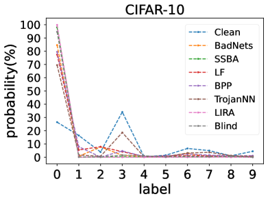
(a)

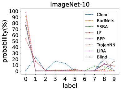
(b)

Figure 6: The label probability distribution within decision boundaries of clean and backdoor models on CIFAR-10 and ImageNet-10, both of whose infected labels are 0.

4.3 Determine the Target Label

After detecting, if the attack is conducted by all-to-one strategy, defenders can further determine the target attacked label by identifying the label with an abnormally high probability in label probability distribution $\mathcal{P}_{k}=\{p_{1},...,p_{m},...,p_{n}\}$. For example, we plot decision boundaries of clean models and backdoor models infected by different backdoor attacks on CIFAR-10 and ImageNet-10 datasets. For each model, we plot 20 decision boundaries and calculate the average label probability. As shown in Fig. 6, the attacked target label (label “0” of both CIFAR-10 and ImageNet-10) exhibits an exceptionally high probability, even reaching 80% to 90% of the entire label probability distribution.

Dataset	Attack→	BadNets	SSBA	LF	BPP	TrojanNN	LIRA	Blind	Worst	Average    [t]
Architecture	Mothod↓									[b]
CIFAR-10	Neural Cleanse	0.881	0.755	0.874	0.881	0.566	0.884	0.535	0.535	0.768    [t]
	MNTD	0.525	0.665	0.568	0.565	0.568	0.623	0.705	0.525	0.603
	MM-BD	1.000	0.847	0.882	0.805	0.860	0.953	0.697	0.697	0.863
PreActResNet-18	Ours-RE	0.995	1.000	0.812	0.762	0.740	1.000	0.919	0.740	0.890
	Ours-ATS	1.000	1.000	0.763	0.747	0.848	1.000	0.885	0.747	0.892    [b]
GTSRB	Neural Cleanse	0.997	0.968	0.937	0.965	0.661	0.715	0.990	0.661	0.890    [t]
	MNTD	0.603	0.495	0.578	0.617	0.535	0.715	0.460	0.460	0.572
	MM-BD	1.000	0.477	0.494	0.445	0.792	0.994	0.997	0.445	0.743
MobileNet-V3	Ours-RE	0.997	0.981	0.942	1.000	0.976	1.000	1.000	0.942	0.985
-Large	Ours-ATS	0.998	0.997	0.972	0.982	0.902	0.996	1.000	0.902	0.978    [b]
CIFAR-100	Neural Cleanse	0.975	0.882	0.811	0.807	0.970	0.970	0.700	0.700	0.874    [t]
	MNTD	0.625	0.490	0.540	0.528	0.540	0.813	0.538	0.490	0.582
	MM-BD	0.626	0.552	0.977	0.557	0.618	0.957	0.633	0.552	0.703
PreActResNet-34	Ours-RE	1.000	1.000	1.000	0.832	0.746	0.979	0.819	0.746	0.911
	Ours-ATS	1.000	1.000	1.000	0.900	0.997	0.988	0.977	0.900	0.980    [b]
ImageNet-10	Neural Cleanse	0.955	0.808	0.683	0.927	0.847	0.969	0.913	0.683	0.872    [t]
	MNTD	0.588	0.428	0.620	0.323	0.620	0.632	0.478	0.323	0.527
	MM-BD	0.107	0.205	0.135	0.120	0.215	0.518	0.149	0.107	0.207
ViT-B-16	Ours-RE	0.956	0.860	0.835	0.913	0.725	1.000	0.863	0.725	0.879
	Ours-ATS	1.000	0.861	0.956	0.976	0.878	1.000	0.935	0.878	0.944    [b]

Table 3: The performance of Model X-ray across different attacks, datasets, and architectures. The last two columns show the worst and the average performance among different attacks. The best results are in bold.

5 Experiment

5.1 Experimental Settings

Datasets and Architectures. The datasets include CIFAR-10 (Krizhevsky et al., 2009), CIFAR-100 (Krizhevsky et al., 2009), GTSRB (Houben et al., 2013), and ImageNet-10 (Howard, ), a subset of ten classes from ImageNet (Deng et al., 2009). Besides, we employ four different architectures: PreActResNet-18 (He et al., 2016), MobileNet-V3-Large (Howard et al., 2019), PreActResNet-34 (He et al., 2016), and ViT-B-16 (Dosovitskiy et al., 2020). These architectures encompass both Convolutional Neural Networks (CNNs) and Vision Transformers (ViTs) and span across various network sizes, including small, medium, and large networks.

Implementation Details. For the model to be evaluated, we plot decision boundaries by random samples triplet with expansion factor $\eta=5$ and density $S=100$, number of plots $N=20$. For the attack baselines, we evaluate our method against seven backdoor attacks, including BadNets (Gu et al., 2017), SSBA (Li et al., 2021a), LF (Zeng et al., 2021), BPP (Wang et al., 2022), TrojanNN (Liu et al., 2018), LIRA (Doan et al., 2021), and Blind (Bagdasaryan & Shmatikov, 2021). We follow an open-sourced backdoor benchmark BackdoorBench (Wu et al., 2022) for the training settings of these attacks and conduct all-to-one attacks by default. As shown in Table 2, the attacks in our experiments contain diverse complex trigger pattern types. In this paper, we focus on backdoor detection for MLaaS. We compare with three post-training detection methods, namely, Neural Cleanse (Wang et al., 2019), MNTD (Xu et al., 2021) and MM-BD (Wang et al., 2023).

Evaluation Metrics. For clean models and models infected by 7 backdoor attacks, we trained 20 models using different initialization and random seeds. For the backdoored models, we select different attack target labels and conduct the single-label attack by default. Considering the computational cost, we adopted different data sets and corresponding common model architectures. Thus, we have $20+20\times 7=160$ models for each combination of dataset and architecture. In subsequent experiments, for each model to be evaluated, we calculate its average RE (see Eq. (3)) and ATS (see Eq. (4)) over $N=20$ decision boundary plots as indicators. We assume that defense mechanisms return a positive label if they identify a model as a backdoored model and then compute the Area Under Receiver Operating Curve (AUROC) to measure the trade-off between the false positive rate (FPR) for clean models and true positive rate (TPR) for backdoor models for a detection method.

(a) CIFAR-10

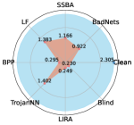
(b) GTSRB

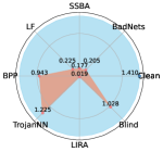
(c) CIFAR-100

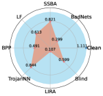
(d) ImageNet-10

Figure 7: The average RE ($\alpha=10$) for clean and backdoor models injected by seven backdoor attacks in CIFAR-10, CIFAR-100, GTSRB, and ImageNet-10 datasets. We observe that backdoor models have significantly smaller RE than clean models.

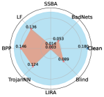
(a) CIFAR-10

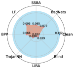
(b) GTSRB

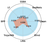
(c) CIFAR-100

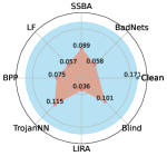
(d) ImageNet-10

Figure 8: The average ATS ($t=0.5$) for clean and backdoor models injected by seven backdoor attacks in CIFAR-10, CIFAR-100, GTSRB, and ImageNet-10 datasets. We observe that backdoor models have significantly smaller ATS than clean models.

5.2 The Effectiveness of Model X-ray

As shown in Table 3, in most cases, Model X-ray outperforms the baseline methods across different backdoor attacks, datasets, and architectures. Notably, the training results for the meta-classifier exhibit some degree of instability. The reported MNTD results represent the best outcomes selected from five independent runs. Neural Cleanse demonstrates promising performance in the majority of scenarios. However, occasional failures may arise when it incorrectly identifies a trigger for a clean model, leading to convergence in local optima. Crucially, Model X-ray stands out as the sole effective method for MLaaS scenarios, whereas Neural Cleanse necessitates access to the model’s parameters, and MNTD relies on soft predictions from the target API. In Fig. 7 and Fig. 8, we provide visual illustrations of the average RE and ATS among both clean and backdoored models. In most cases, a clear distinction is evident, except for LF, BBP, and TrojanNN on CIFAR-10, which aligns with the quantitative results presented in Table 3. Employing improved analysis strategies may help address this issue.

5.3 The Efficiency of Model X-ray

In Table 4, we show the number of benign samples that the defender needs. Both Neural Cleanse and MNTD necessitate a certain proportion of benign data (e.g., 5% of the benign dataset) to complement their defense mechanisms. In contrast, our method necessitates only three benign samples to plot a decision boundary, and with $N$ set to 20, only 60 clean samples are required, which is already sufficient to ensure the effectiveness of our detection. In addition, we compare the average evaluation execution time of each method on CIFAR-10 dataset in Table 5. The experiment is conducted on one NVIDIA RTX A6000. Specifically, Neural Cleanse requires a trigger reverse engineering optimization process, MM-BD also requires an optimization process and MNTD requires preparation that generates a large set of shadow models (1024 clean models and 1024 attack models) to train a meta-classifier. In contrast, our method does not demand any optimization or training processes, making it a versatile and plug-and-play solution.

Method	CIFAR-10	GTSRB	CIFAR-100	ImageNet-10
Neural Cleanse	2500	1332	2500	473
MNTD	2500	1332	2500	473
MM-BD	0	0	0	0
Ours	60	60	60	60

Table 4: Benign samples required for different methods.

Method	Neural Cleanse	MNTD $\dagger$	MNTD	MM-BD	Ours
Time (s)	243.4	44268.6	0.08	75.2	36.5

Table 5: Execution time on CIFAR-10. $\dagger$ means the training time.

5.4 threshold

Since Model X-ray maps the model to a linearly separable space and defenders make judgments based on a threshold $\gamma$. Observing the RE and ATS of clean and backdoor models with different architectures on the same dataset (see Fig. 9 and Fig. 10), we find that detection between models in the same dataset on different architectures exhibits transferability. This allows us to empirically determine a threshold $\gamma$.

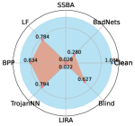
(a) PreActResNet18

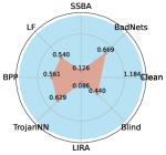
(b) MobileNet-L

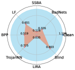
(c) PreActResNet34

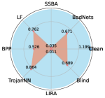
(d) VGG19

Figure 9: The average RE($\alpha=10$) for clean and backdoor models injected by seven backdoor attacks in CIFAR-10 on different architectures.

(a) PreActResNet18

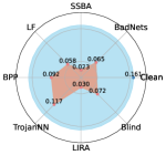
(b) MobileNet-L

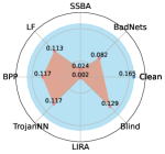
(c) PreActResNet34

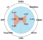
(d) VGG19

Figure 10: The average ATS($t=0.5$) for clean and backdoor models injected by seven backdoor attacks in CIFAR-10 on different architectures.

5.5 Ablation Study

The Influence of the Hyper-parameters. $N$ is the number of decision boundary plots and $S$ is the density of decision boundaries, which are critical to the evaluation efficiency. Here, we investigate Model X-ray ’s performance under fixed $N=20$ with $S$ ranging from 60 to 140 and under fixed $S=100$ with $N$ ranging from 5 to 40. Fig. 11 shows that lower $N$ and $S$ will slightly degrade the performance of Model X-ray on CIFAR-10, which is still acceptable.

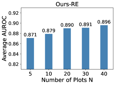
(a)

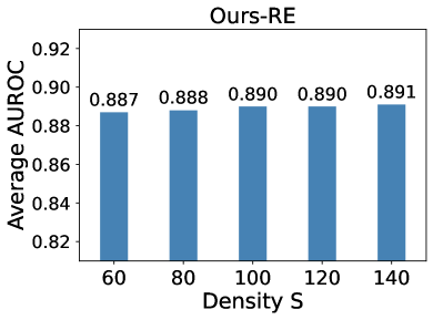
(b)

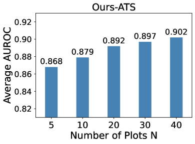
(c)

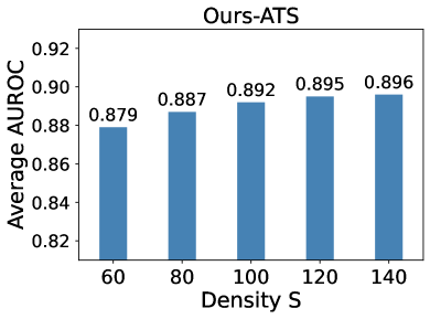
(d)

Figure 11: The influence of the number of plots $N$ and density $S$.

Besides, we investigate the impact of parameters in two indicators, i.e., $\alpha$ in RE and $t$ in ATS. As shown in Fig. 12, different $\alpha$ has a neglectable effect on Ours-RE, while $t$ larger than 0.5 is better for Ours-ATS.

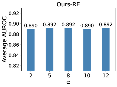
(a)

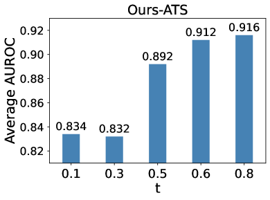
(b)

Figure 12: The influence of the parameters $\alpha$ and $t$.

The Influence of the Poisoning Ratio. In the above experiment, we set the poisoning ratio as 10% by default. Here, we further evaluate our method against data-poisoning attacks under different poisoning ratios (1%, 5%, 10%, and 20%) on CIFAR-10 dataset. As shown in Fig. 13, as the poisoning ratio increases, our approach becomes more effective, indicating that the phenomenon of anomalous decision boundaries in the backdoor models becomes more pronounced. For low ratios like 1%, the attack ability for some attacks degrades, wherein the poorer performance is understood.

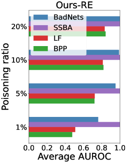
(a)

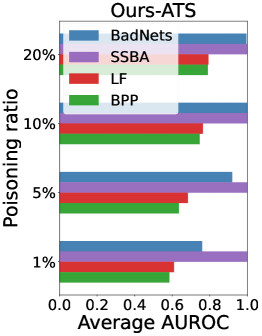
(b)

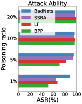
(c)

Figure 13: The influence of the poisoning ratio.

The Impact of Different Attack Strategies. Besides the default all-to-one attack strategy, we consider the X2X attack strategy (Xiang et al., 2023), with arbitrary numbers of source classes each assigned with an arbitrary target class, including X-to-X attack, X-to-one attack, and one-to-one attack. We adopt different attack strategies to conduct BadNets on CIFAR-10. For each strategy, we train 10 models for evaluation. Table 6 shows that Model X-ray remains effective under different attack strategies, especially based on ATS (i.e., Ours-ATS). Furthermore, we provide some visual examples of the corresponding decision boundary in Fig. 14. Taking 10-to-10 as an example, wherein all labels are injected, the area for triple clean samples shrinks, indicating the degraded robustness of clean samples.

Strategy	10to1	5to1	2to1	1to1	3to3	5to5	10to10
Neural Cleanse	0.881	0.845	0.784	0.826	0.423	0.284	0.439 [t]
MNTD	0.525	0.419	0.503	0.487	0.535	0.518	0.466
MM-BD	1.000	0.571	0.006	0.081	0.007	0.448	0.671
Ours-RE	1.000	0.995	0.824	0.829	0.839	0.638	0.423
Ours-ATS	1.000	0.995	0.967	0.862	0.821	0.862	0.746 [b]

Table 6: The performance under different attack strategies.

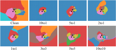
Figure 14: Decision boundaries under different attack strategies.

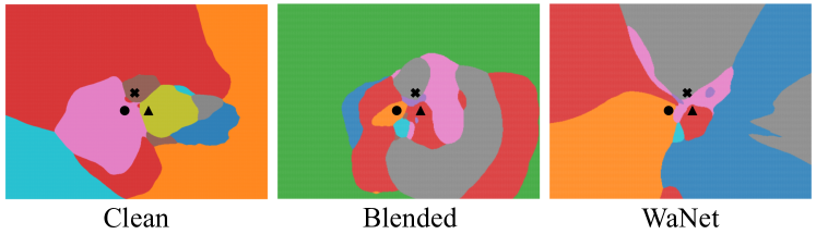
Figure 15: Decision boundaries of Blended (Chen et al., 2017) and WaNet (Nguyen & Tran, 2021).

6 Discussion

Special Cases. We find that Ours-AST can distinguish the backdoored model by WaNet (Nguyen & Tran, 2021) from the clean model. Differently, the AST of WaNet is larger rather than smaller than that of the clean model (see Fig. 15). We conjecture that WaNet can be seen as an augmentation enhancing the robustness of clean samples. Blended (Chen et al., 2017) can bypass our detection. We explain that blending the trigger pattern with clean samples may not establish the shortcuts because of the redundancy of the model, which can be easily purified by pruning like ANP (Wu & Wang, 2021). Nonetheless, we need more sophisticated strategies to achieve better detection for MLaaS.

CIFAR-10	Balanced	IF=100	IF=50	IF=10
RE	1.081	0.987	1.025	1.074
ATS	0.180	0.165	0.180	0.203

Table 7: The RE and ATS of clean models trained on the balanced and unbalanced CIFAR-10. IF denotes the imbalance factor.

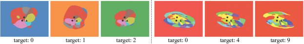
(a)

Figure 16: The detection of clean-label attacked models in CIFAR-10 [left] and BadNets attacked models in Tiny-ImageNet200 [right].

The detection against clean-label attacks. As shown in Figure 16-left, our method still identifies the overwhelming regions of target labels within the decision boundaries. We explain that clean-label attacks also make the decision boundary distinguishable.

Evaluation on Tiny-ImageNet200. As shown in Figure 16-right, Model X-ray still identifies the overwhelming regions of target labels (different red colors).

The decision boundaries constructed by noisy images or adversarial samples. As shown in Figure 17, introducing Gaussian noise and FGSM adversarial perturbations to images may lead to slight fragmentation in the decision boundaries. The introduction of noise and perturbations has a minimal impact on the detection, highlighting that it doesn’t necessarily require entirely clean samples.

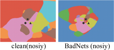
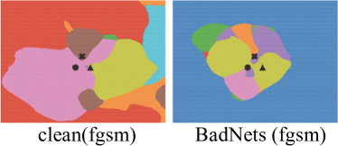
(a)

Figure 17: The decision boundaries constructed by noisy samples [left] and adversarial samples [right].

Decision Boundaries of Clean Models on Unbalanced Dataset. Here, we adopt GLMC (Du et al., 2023), a method for long-tailed visual recognitions to train clean models on Unbalanced CIFAR-10 under different imbalance factors (IFs). As shown in Table 7, the RE and ATS for balanced CIFAR-10 and imbalanced CIFAR-10 are very similar, which means that the proposed method is not impacted by whether the dataset is balanced (refer to Figure 18).

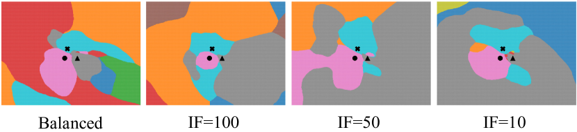
Figure 18: Decision boundaries of clean models trained on the balanced and unbalanced CIFAR-10.

7 Conclusion

In this paper, we propose Model X-ray , a backdoor detection for MLaaS via decision boundary, which solely relies on the hard prediction of clean inputs and can determine the target label under the all-to-one attack strategy. Extensive experiments support that Model X-ray has outstanding effectiveness and efficiency against diverse backdoor attacks on different datasets, and architectures.

Appendix A Implementation Details

A.1 Details of Datasets

Table 8 shows the details of four datasets for evaluation.

Dataset	Classes	Image Size	Training Data	Test Data
CIFAR-10	10	3×32×32	50,000	10,000
GTSRB	43	3×32×32	39,209	12,630
CIFAR-100	100	3×32×32	50,000	10,000
ImageNet-10	10	3×160×160	9,469	3,925

Table 8: The datasets for evaluation

A.2 Details of Training Configurations

Following an open-sourced backdoor benchmark (Wu et al., 2022), we use the same training configuration to train both clean and backdoored models. These details are shown in Table 9.

Configurations	CIFAR-10	GTSRB	CIFAR-100	ImageNet-10
Model	PreActResNet-18	MobileNet-V3-Large	PreActResNet-34	ViT-B-16
Optimizer	SGD	SGD	SGD	SGD
SGD Momentum	0.9	0.9	0.9	0.9
Batch Size	128	128	128	128
Learning Rate	0.01	0.01	0.01	0.01
Scheduler	CosineAnnealing	CosineAnnealing	CosineAnnealing	CosineAnnealing
Weight Decay	0.0005	0.0005	0.0005	0.0005
Epochs	50	50	50	50

Table 9: The training configurations for both clean and backdoored models.

A.3 Details of Attacks Configurations

For backdoored models, we conduct all-to-one attacks by randomly choosing the attack target label. For poisoning-based attacks, we set the default poisoning ratio as 10%, for model modification-based attacks, we adopt its default implementation in (Wu et al., 2022).

The attacks involved in our evaluations contain diverse complex trigger pattern types, including patch, invisible, and input-aware triggers. Fig. 19 shows some visual examples of trigger samples generated by diverse backdoor attacks involved in our evaluations. Table 10 shows attack ability for diverse backdoor attacks on different datasets and architectures, indicating that all the attacks are effective.

Dataset	Architecture	Clean	BadNets		SSBA		LF		BPP		TrojanNN		LIRA		Blind
		ACC	ACC	ASR	ACC	ASR	ACC	ASR	ACC	ASR	ACC	ASR	ACC	ASR	ACC	ASR
CIFAR-10	PreActResNet-18	0.925	0.913	0.963	0.902	0.955	0.906	0.969	0.910	0.964	0.917	0.999	0.648	0.806	0.845	0.950
GTSRB	MobileNet-V3	0.904	0.891	0.922	0.905	0.853	0.905	0.995	0.889	0.823	0.908	0.999	0.129	0.951	0.787	0.791
	-Large
CIFAR-100	PreActResNet-34	0.712	0.664	0.915	0.692	0.968	0.682	0.954	0.660	0.985	0.695	0.999	0.158	0.984	0.562	0.999
ImageNet-10	ViT-B-16	0.985	0.983	0.997	0.984	0.993	0.869	0.804	0.963	0.958	0.984	0.998	0.942	0.965	0.982	0.999

Table 10: The average accuracy (ACC) and attack success rate (ASR) for different backdoored models on different datasets and architectures.

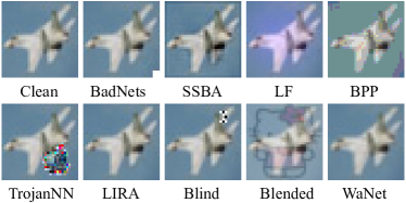
Figure 19: Some visual examples of trigger samples for different backdoor attacks.

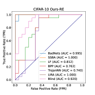
(a)

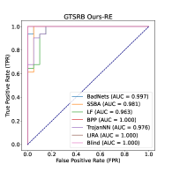
(b)

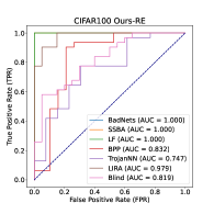
(c)

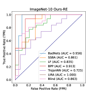
(d)

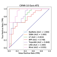
(e)

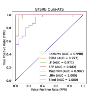
(f)

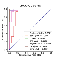
(g)

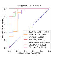
(h)

Figure 20: The ROC curves of Ours-RE [top] and Ours-ATS [bottom] against seven backdoor attacks on CIFAR-10, GTSRB, CIFAR-100, and ImageNet-10.

A.4 Details of the Defense Baselines

As shown in Figure 20, we present the ROC curves of our methods. For Neural Cleanse (Wang et al., 2019), we adopt its default implementation in (Wu et al., 2022). For MNTD (Xu et al., 2021), we adopt its official implementation (mnt, ) to train a meta-classifier based on features extracted from a large set of shadow models (1024 clean models and 1024 attack models) for each combination of dataset and architecture, it means ${2048\times 4=8192}$ shadow models in total. For MM-BD, we adopt its official implementation in (mmb, ).

Appendix B The Influence of Expansion Factor $\eta$ for Plotting Decision Boundary

In the above experiment, we set the value for expansion factor $\eta$ as 5 by default, which is an intuitive choice. In subsequent experiments, we observed anomalous decision boundary phenomena in certain attacks occurring over a larger range, such as in LF, BPP, and TrojanNN. Therefore, choosing a larger value for $\eta$ can enhance the performance of Ours-RE. Here, we further evaluate Ours-RE by setting expansion factor $\eta$ as 8 on CIFAR-10 dataset. As shown in Table 11, a larger value for $\eta$ can enhance the performance of Ours-RE.

Ours-RE	BadNets	SSBA	LF	BPP	TrojanNN	LIRA	Blind	Average
$\eta=5$	0.995	1.000	0.812	0.762	0.740	1.000	0.919	0.890
$\eta=8$	0.982	1.000	0.910	0.863	0.798	1.000	0.911	0.923

Table 11: The influence of expansion factor $\eta$.

Appendix C Evaluations on Open-source Benchmarks

To mitigate the impact of incidental factors in our training, we also evaluated our method on the backdoored models pre-trained on an open-source benchmark (Wu et al., 2022). Specifically, we conduct empirical evaluations on pre-trained backdoored models injected by seven backdoor attacks across CIFAR-10, GTSRB and CIFAR-100 datasets on the PreActResNet-18 architecture, which can be downloaded from (Bac, ). As shown in Fig. 21, our method consistently identifies anomalies in the decision boundaries that triple samples are encircled by a large area of the target label, demonstrating precise detection of backdoored models and determine the attack target labels.

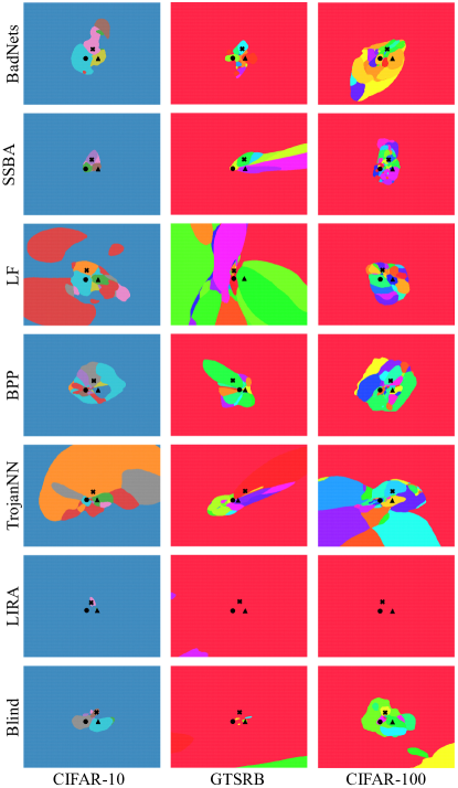
Figure 21: Evaluation results for backdoored models on CIFAR-10, GTSRB, and CIFAR-100 using PreActResNet-18 pre-trained on an open-source benchmark (Bac, ).

Appendix D More Visual Examples of Decision Boundaries for Backdoored Models

In our main manuscript, we only presented decision boundaries for a few examples of backdoored models due to space constraints. As shown in Fig. 22h, Fig. 22h, Fig. 22h and Fig. 22h, we showcase decision boundaries for diverse backdoored models with different attack target labels (from label: 0 to label: 9 in all the datasets), including different datasets and architectures involved in our evaluations. As we can see, by arbitrarily selecting the attack target label, the corresponding target label significantly influences the decision region that the prediction distribution within the decision boundary of the backdoored model is more gathered, and triple samples are encircled by a large area of the target label.

Figure 22: More visual examples of decision boundaries for backdoored models in CIFAR-10.

(a) The color-class schema for CIFAR-10

(b) CIFAR-10 BadNets

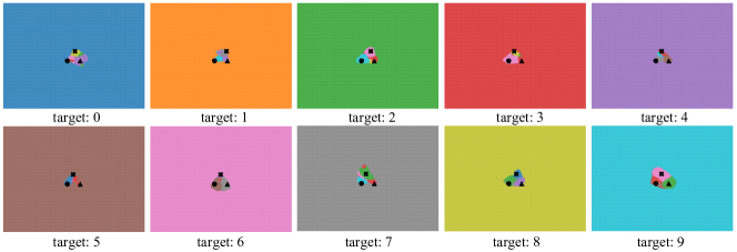
(c) CIFAR-10 SSBA

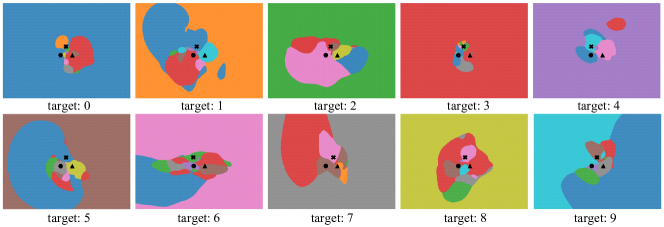
(d) CIFAR-10 LF

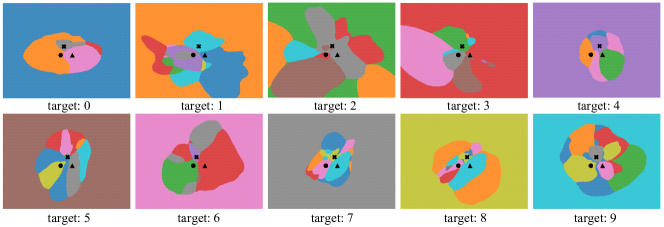
(e) CIFAR-10 BPP

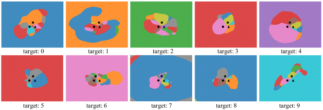
(f) CIFAR-10 TrojanNN

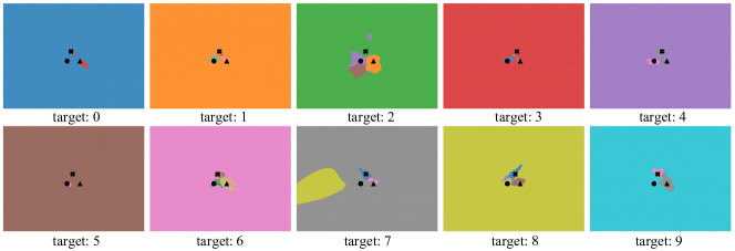
(g) CIFAR-10 LIRA

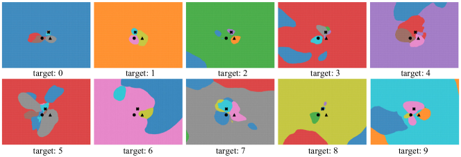
(h) CIFAR-10 Blind

Figure 22: More visual examples of decision boundaries for backdoored models in ImageNet-10.

(a) The color-class schema for ImageNet-10

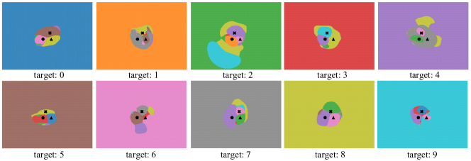
(b) ImageNet-10 BadNets

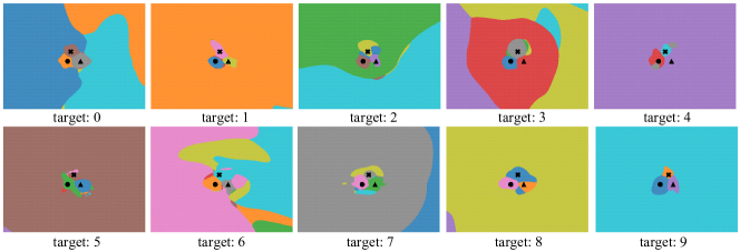
(c) ImageNet-10 SSBA

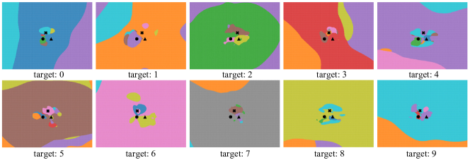
(d) ImageNet-10 LF

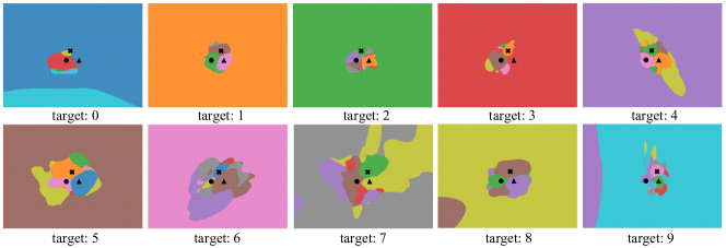
(e) ImageNet-10 BPP

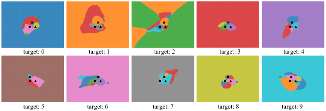
(f) ImageNet-10 TrojanNN

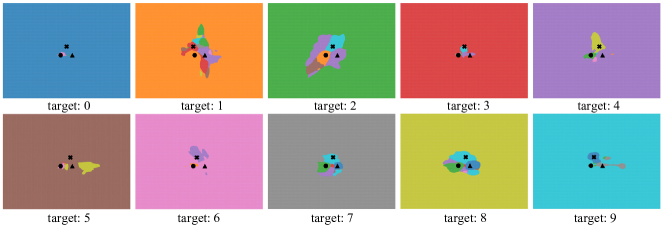
(g) ImageNet-10 LIRA

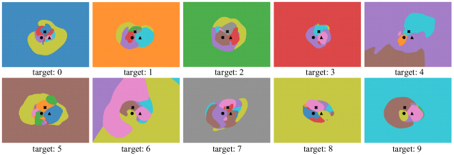
(h) ImageNet-10 Blind

Figure 22: More visual examples of decision boundaries for backdoored models in GTSRB.

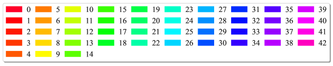
(a) The color-class schema for GTSRB

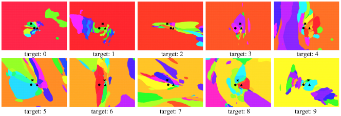
(b) GTSRB BadNets

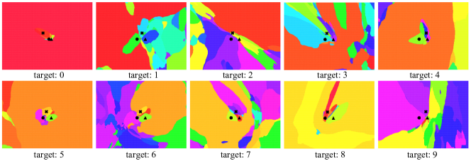
(c) GTSRB SSBA

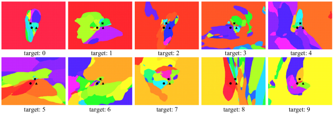
(d) GTSRB LF

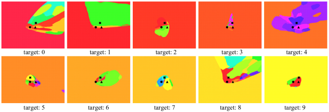
(e) GTSRB BPP

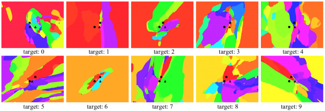
(f) GTSRB TrojanNN

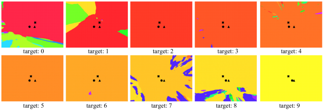
(g) GTSRB LIRA

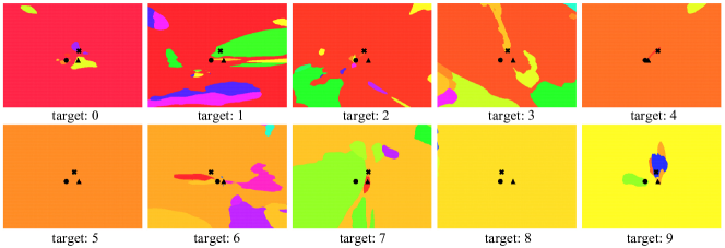
(h) GTSRB Blind

Figure 22: More visual examples of decision boundaries for backdoored models in CIFAR100.

(a) The color-class schema for CIFAR100

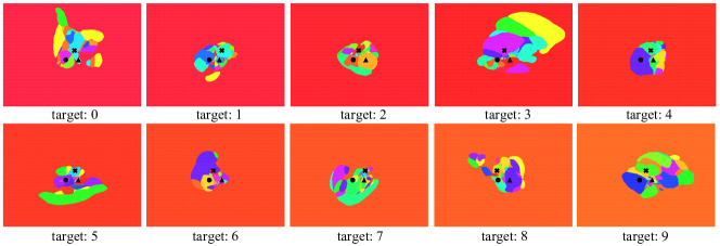
(b) CIFAR100 BadNets

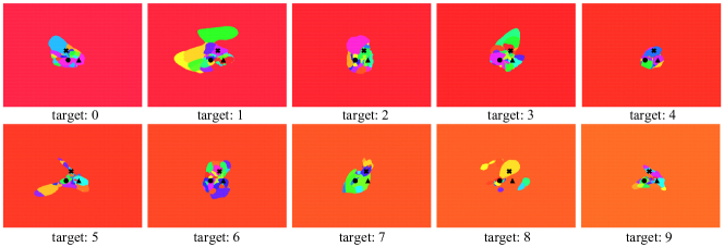
(c) CIFAR100 SSBA

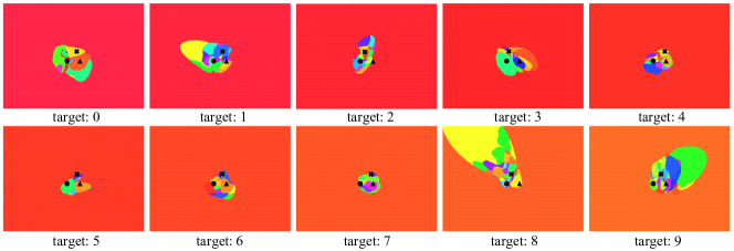
(d) CIFAR100 LF

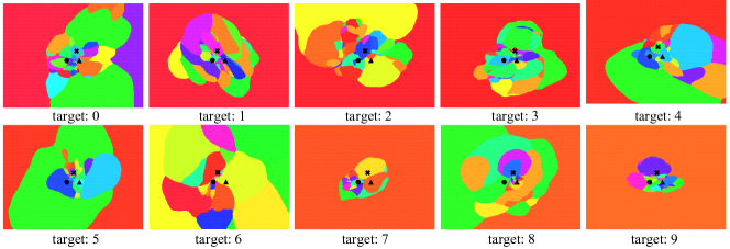
(e) CIFAR100 BPP

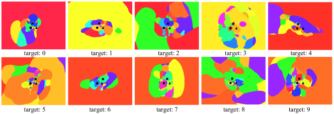
(f) CIFAR100 TrojanNN

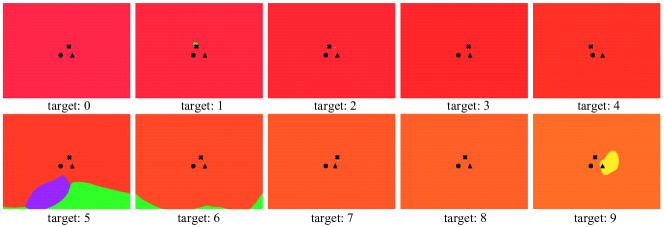
(g) CIFAR100 LIRA

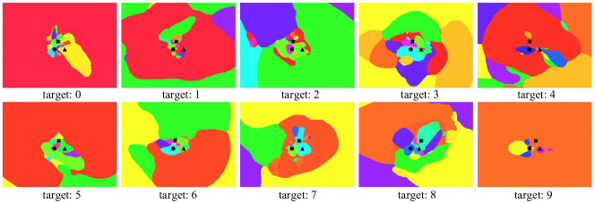
(h) CIFAR100 Blind

References

- (1) Github: Backdoorbench. URL https://github.com/SCLBD/BackdoorBench.
- (2) Github: Mm-bd. URL https://github.com/wanghangpsu/MM-BD.
- (3) Github: Meta-nerual-trojan-detection. URL https://github.com/AI-secure/Meta-Nerual-Trojan-Detection.
- (4) Rényi entropy. https://en.wikipedia.org/wiki/R
- Bagdasaryan & Shmatikov (2021) Bagdasaryan, E. and Shmatikov, V. Blind backdoors in deep learning models. In 30th USENIX Security Symposium (USENIX Security 21), pp. 1505–1521, 2021.
- Barni et al. (2019) Barni, M., Kallas, K., and Tondi, B. A new backdoor attack in cnns by training set corruption without label poisoning. In 2019 IEEE International Conference on Image Processing (ICIP), pp. 101–105. IEEE, 2019.
- Chen et al. (2018) Chen, B., Carvalho, W., Baracaldo, N., Ludwig, H., Edwards, B., Lee, T., Molloy, I., and Srivastava, B. Detecting backdoor attacks on deep neural networks by activation clustering. arXiv preprint arXiv:1811.03728, 2018.
- Chen et al. (2019) Chen, H., Fu, C., Zhao, J., and Koushanfar, F. Deepinspect: A black-box trojan detection and mitigation framework for deep neural networks. In IJCAI, volume 2, pp. 8, 2019.
- Chen et al. (2017) Chen, X., Liu, C., Li, B., Lu, K., and Song, D. Targeted backdoor attacks on deep learning systems using data poisoning. arXiv preprint arXiv:1712.05526, 2017.
- Cohen et al. (2019) Cohen, J., Rosenfeld, E., and Kolter, Z. Certified adversarial robustness via randomized smoothing. In international conference on machine learning, pp. 1310–1320. PMLR, 2019.
- Deng et al. (2009) Deng, J., Dong, W., Socher, R., Li, L.-J., Li, K., and Fei-Fei, L. Imagenet: A large-scale hierarchical image database. In 2009 IEEE conference on computer vision and pattern recognition, pp. 248–255. Ieee, 2009.
- Doan et al. (2021) Doan, K., Lao, Y., Zhao, W., and Li, P. Lira: Learnable, imperceptible and robust backdoor attacks. In Proceedings of the IEEE/CVF international conference on computer vision, pp. 11966–11976, 2021.
- Dong et al. (2021) Dong, Y., Yang, X., Deng, Z., Pang, T., Xiao, Z., Su, H., and Zhu, J. Black-box detection of backdoor attacks with limited information and data. In Proceedings of the IEEE/CVF International Conference on Computer Vision, pp. 16482–16491, 2021.
- Dosovitskiy et al. (2020) Dosovitskiy, A., Beyer, L., Kolesnikov, A., Weissenborn, D., Zhai, X., Unterthiner, T., Dehghani, M., Minderer, M., Heigold, G., Gelly, S., et al. An image is worth 16x16 words: Transformers for image recognition at scale. arXiv preprint arXiv:2010.11929, 2020.
- Du et al. (2023) Du, F., Yang, P., Jia, Q., Nan, F., Chen, X., and Yang, Y. Global and local mixture consistency cumulative learning for long-tailed visual recognitions. In Proceedings of the IEEE/CVF Conference on Computer Vision and Pattern Recognition, pp. 15814–15823, 2023.
- Esteva et al. (2017) Esteva, A., Kuprel, B., Novoa, R. A., Ko, J., Swetter, S. M., Blau, H. M., and Thrun, S. Dermatologist-level classification of skin cancer with deep neural networks. nature, 542(7639):115–118, 2017.
- Fu et al. (2023) Fu, C., Zhang, X., Ji, S., Wang, T., Lin, P., Feng, Y., and Yin, J. Freeeagle: Detecting complex neural trojans in data-free cases. arXiv preprint arXiv:2302.14500, 2023.
- Gao et al. (2019) Gao, Y., Xu, C., Wang, D., Chen, S., Ranasinghe, D. C., and Nepal, S. Strip: A defence against trojan attacks on deep neural networks. In Proceedings of the 35th Annual Computer Security Applications Conference, pp. 113–125, 2019.
- Graves et al. (2013) Graves, A., Mohamed, A.-r., and Hinton, G. Speech recognition with deep recurrent neural networks. In 2013 IEEE international conference on acoustics, speech and signal processing, pp. 6645–6649. Ieee, 2013.
- Gu et al. (2017) Gu, T., Dolan-Gavitt, B., and Garg, S. Badnets: Identifying vulnerabilities in the machine learning model supply chain. arXiv preprint arXiv:1708.06733, 2017.
- Guo et al. (2021) Guo, J., Li, A., and Liu, C. Aeva: Black-box backdoor detection using adversarial extreme value analysis. arXiv preprint arXiv:2110.14880, 2021.
- Guo et al. (2023) Guo, J., Li, Y., Chen, X., Guo, H., Sun, L., and Liu, C. Scale-up: An efficient black-box input-level backdoor detection via analyzing scaled prediction consistency. arXiv preprint arXiv:2302.03251, 2023.
- He et al. (2016) He, K., Zhang, X., Ren, S., and Sun, J. Identity mappings in deep residual networks. In Computer Vision–ECCV 2016: 14th European Conference, Amsterdam, The Netherlands, October 11–14, 2016, Proceedings, Part IV 14, pp. 630–645. Springer, 2016.
- He et al. (2018) He, W., Li, B., and Song, D. Decision boundary analysis of adversarial examples. In International Conference on Learning Representations, 2018.
- He et al. (2019) He, Z., Zhang, T., and Lee, R. Sensitive-sample fingerprinting of deep neural networks. In Proceedings of the IEEE/CVF conference on computer vision and pattern recognition, pp. 4729–4737, 2019.
- Houben et al. (2013) Houben, S., Stallkamp, J., Salmen, J., Schlipsing, M., and Igel, C. Detection of traffic signs in real-world images: The german traffic sign detection benchmark. In The 2013 international joint conference on neural networks (IJCNN), pp. 1–8. Ieee, 2013.
- Howard et al. (2019) Howard, A., Sandler, M., Chu, G., Chen, L.-C., Chen, B., Tan, M., Wang, W., Zhu, Y., Pang, R., Vasudevan, V., et al. Searching for mobilenetv3. In Proceedings of the IEEE/CVF international conference on computer vision, pp. 1314–1324, 2019.
- (28) Howard, J. Github: imagenette. URL https://github.com/fastai/imagenette/.
- Khoury & Hadfield-Menell (2018) Khoury, M. and Hadfield-Menell, D. On the geometry of adversarial examples. arXiv preprint arXiv:1811.00525, 2018.
- Krizhevsky et al. (2009) Krizhevsky, A., Hinton, G., et al. Learning multiple layers of features from tiny images. 2009.
- Krizhevsky et al. (2012) Krizhevsky, A., Sutskever, I., and Hinton, G. E. Imagenet classification with deep convolutional neural networks. Advances in neural information processing systems, 25, 2012.
- Li et al. (2021a) Li, Y., Li, Y., Wu, B., Li, L., He, R., and Lyu, S. Invisible backdoor attack with sample-specific triggers. In Proceedings of the IEEE/CVF international conference on computer vision, pp. 16463–16472, 2021a.
- Li et al. (2021b) Li, Y., Lyu, X., Koren, N., Lyu, L., Li, B., and Ma, X. Anti-backdoor learning: Training clean models on poisoned data. Advances in Neural Information Processing Systems, 34:14900–14912, 2021b.
- Liu et al. (2023) Liu, X., Li, M., Wang, H., Hu, S., Ye, D., Jin, H., Wu, L., and Xiao, C. Detecting backdoors during the inference stage based on corruption robustness consistency. In Proceedings of the IEEE/CVF Conference on Computer Vision and Pattern Recognition, pp. 16363–16372, 2023.
- Liu et al. (2018) Liu, Y., Ma, S., Aafer, Y., Lee, W.-C., Zhai, J., Wang, W., and Zhang, X. Trojaning attack on neural networks. In 25th Annual Network And Distributed System Security Symposium (NDSS 2018). Internet Soc, 2018.
- Liu et al. (2019) Liu, Y., Lee, W.-C., Tao, G., Ma, S., Aafer, Y., and Zhang, X. Abs: Scanning neural networks for back-doors by artificial brain stimulation. In Proceedings of the 2019 ACM SIGSAC Conference on Computer and Communications Security, pp. 1265–1282, 2019.
- Nguyen & Tran (2021) Nguyen, A. and Tran, A. Wanet–imperceptible warping-based backdoor attack. arXiv preprint arXiv:2102.10369, 2021.
- Parkhi et al. (2015) Parkhi, O., Vedaldi, A., and Zisserman, A. Deep face recognition. In BMVC 2015-Proceedings of the British Machine Vision Conference 2015. British Machine Vision Association, 2015.
- Rajabi et al. (2023) Rajabi, A., Asokraj, S., Jiang, F., Niu, L., Ramasubramanian, B., Ritcey, J., and Poovendran, R. Mdtd: A multi domain trojan detector for deep neural networks. arXiv preprint arXiv:2308.15673, 2023.
- Redmon et al. (2016) Redmon, J., Divvala, S., Girshick, R., and Farhadi, A. You only look once: Unified, real-time object detection. In Proceedings of the IEEE conference on computer vision and pattern recognition, pp. 779–788, 2016.
- Somepalli et al. (2022) Somepalli, G., Fowl, L., Bansal, A., Yeh-Chiang, P., Dar, Y., Baraniuk, R., Goldblum, M., and Goldstein, T. Can neural nets learn the same model twice? investigating reproducibility and double descent from the decision boundary perspective. In Proceedings of the IEEE/CVF Conference on Computer Vision and Pattern Recognition, pp. 13699–13708, 2022.
- Tang et al. (2021) Tang, D., Wang, X., Tang, H., and Zhang, K. Demon in the variant: Statistical analysis of DNNs for robust backdoor contamination detection. In 30th USENIX Security Symposium (USENIX Security 21), pp. 1541–1558, 2021.
- Tran et al. (2018) Tran, B., Li, J., and Madry, A. Spectral signatures in backdoor attacks. Advances in neural information processing systems, 31, 2018.
- Wang et al. (2019) Wang, B., Yao, Y., Shan, S., Li, H., Viswanath, B., Zheng, H., and Zhao, B. Y. Neural cleanse: Identifying and mitigating backdoor attacks in neural networks. In 2019 IEEE Symposium on Security and Privacy (SP), pp. 707–723. IEEE, 2019.
- Wang et al. (2023) Wang, H., Xiang, Z., Miller, D. J., and Kesidis, G. Mm-bd: Post-training detection of backdoor attacks with arbitrary backdoor pattern types using a maximum margin statistic. In 2024 IEEE Symposium on Security and Privacy (SP), pp. 15–15. IEEE Computer Society, 2023.
- Wang et al. (2020) Wang, R., Zhang, G., Liu, S., Chen, P.-Y., Xiong, J., and Wang, M. Practical detection of trojan neural networks: Data-limited and data-free cases. In Computer Vision–ECCV 2020: 16th European Conference, Glasgow, UK, August 23–28, 2020, Proceedings, Part XXIII 16, pp. 222–238. Springer, 2020.
- Wang et al. (2022) Wang, Z., Zhai, J., and Ma, S. Bppattack: Stealthy and efficient trojan attacks against deep neural networks via image quantization and contrastive adversarial learning. In Proceedings of the IEEE/CVF Conference on Computer Vision and Pattern Recognition, pp. 15074–15084, 2022.
- Wu et al. (2022) Wu, B., Chen, H., Zhang, M., Zhu, Z., Wei, S., Yuan, D., and Shen, C. Backdoorbench: A comprehensive benchmark of backdoor learning. Advances in Neural Information Processing Systems, 35:10546–10559, 2022.
- Wu & Wang (2021) Wu, D. and Wang, Y. Adversarial neuron pruning purifies backdoored deep models. Advances in Neural Information Processing Systems, 34:16913–16925, 2021.
- Xiang et al. (2023) Xiang, Z., Xiong, Z., and Li, B. Umd: Unsupervised model detection for x2x backdoor attacks. arXiv preprint arXiv:2305.18651, 2023.
- Xu et al. (2021) Xu, X., Wang, Q., Li, H., Borisov, N., Gunter, C. A., and Li, B. Detecting ai trojans using meta neural analysis. In 2021 IEEE Symposium on Security and Privacy (SP), pp. 103–120. IEEE, 2021.
- Zeng et al. (2021) Zeng, Y., Park, W., Mao, Z. M., and Jia, R. Rethinking the backdoor attacks’ triggers: A frequency perspective. 2021 ieee. In CVF International Conference on Computer Vision (ICCV), pp. 16453–16461, 2021.
- Zhang et al. (2017) Zhang, H., Cisse, M., Dauphin, Y. N., and Lopez-Paz, D. mixup: Beyond empirical risk minimization. arXiv preprint arXiv:1710.09412, 2017.