CLAPSep: Leveraging Contrastive Pre-trained Models for Multi-Modal Query-Conditioned Target Sound Extraction

Abstract

Universal sound separation (USS) aims to extract arbitrary types of sounds from real-world sound recordings. Language-queried target sound extraction (TSE) is an effective approach to achieving USS. Such systems consist of two components: a query network that converts user queries into conditional embeddings, and a separation network that extracts the target sound based on conditional embeddings. Existing methods mainly suffer from two issues: firstly, they require training a randomly initialized model from scratch, lacking the utilization of pre-trained models, and substantial data and computational resources are needed to ensure model convergence; secondly, existing methods need to jointly train a query network and a separation network, which tends to lead to overfitting. To address these issues, we build the CLAPSep model based on contrastive language-audio pre-trained model (CLAP). We achieve this by using a pre-trained text encoder of CLAP as the query network and introducing pre-trained audio encoder weights of CLAP into the separation network to fully utilize the prior knowledge embedded in the pre-trained model to assist in target sound extraction tasks. Extensive experimental results demonstrate that the proposed method saves training resources while ensuring the model’s performance and generalizability. Additionally, we explore the model’s ability to comprehensively utilize language/audio multi-modal and positive/negative multi-valent user queries, enhancing system performance while providing diversified application modes.

I Introduction

People possess a remarkable ability to concentrate on specific sound events amid noisy environments, a phenomenon known as the cocktail party effect. This auditory system attribute has been extensively explored across disciplines. In the domain of signal processing, researchers have diligently worked on technologies to address the challenges posed by the cocktail party problem. A significant advancement in this field is the emergence of sound separation [1, 2, 3], a methodology devised to untangle a blend of sounds, isolating individual sources and making them perceptually distinct.

In recent years, the advancement of deep neural networks (DNNs) has led to numerous successful implementations in sound separation. Depending on the types of sounds processed, existing methods can be categorized into speech separation (SS) [1, 4], speech enhancement (SE) [2, 5], music source separation (MSS) [3, 6, 7], and more. Universal sound separation (USS) [8, 9, 10, 11] takes a broader perspective, aiming to separate arbitrary types of sound in real-world recordings. The task’s complexity increases with the growing number of potential sound classes within the mixture, making the separation of each source a daunting task. An alternative strategy to confront this challenge is query-conditioned target sound extraction, focusing on extracting only the target sound described by auxiliary information.

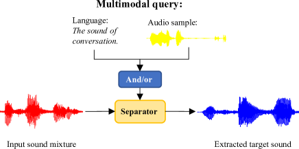
Figure 1: An illustration of query-conditioned target sound extraction.

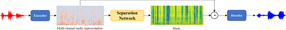
Figure 2: An illustration of mask-based sound separation pipeline, where $\odot$ denotes element-wise production.

In the context of queried-conditioned TSE, the query describing what sound to extract plays a pivotal role in guiding the separation model. Depending on the specific task requirements, the types of queries can be quite diverse. These include label query [12, 13, 14], audio query [8, 14, 15, 16], visual query [17, 18], language query [19, 20, 15], etc. Among them, label query is the simplest, using finite predefined discrete labels to indicate the sound events to be extracted. However, the disadvantage of this approach is quite obvious. It can only extract a limited number of sound events corresponding to the finite predefined labels. This mismatch with the goal of USS is still a gap to be filled. As an alternative to label querying, a more nuanced and sophisticated approach known as language querying is gaining prominence. Unlike label queries, which directly specify the target sound, language queries involve providing a more comprehensive and descriptive instruction. For example, instead of simply specifying “voice” or “instrument”, a language query might include a natural language description such as “A man talking as a stream of water trickles in the background” or “Instrumental music playing as a woman speaks”. The introduction of language queries adds a layer of contextual understanding that allows the separation model to interpret and process instructions in a more human-like manner. This shift from simple labels to richer linguistic instructions improves the model’s adaptability to different scenarios and contributes to a more intuitive and versatile sound separation process.

Previous work [19] attempts to use a pre-trained language model (e.g., BERT [21]) to encode input query text into condition embeddings. These embeddings are then utilized to guide the separation model in executing TSE. The training process involves the joint optimization of both the query model and the separation model. However, training such a model poses significant challenges as it must learn to map the query texts to semantically consistent audio feature embeddings and perform separation conditioned on the learned embeddings simultaneously. Moreover, this straightforward strategy tends to lead the model towards overfitting to queries encountered during its training phase. As a consequence, generalizing to unseen language queries becomes challenging, limiting the model’s adaptability to a broader range of inputs.

The development of contrastive language-audio pre-training [22] models recently makes it possible to decouple the training of query models and separation models. The CLAP model comprises an audio encoder and a text encoder, capable of transforming their respective modality inputs into semantically consistent embeddings. In this way, the pre-trained CLAP text encoder can be directly served as the query model without any finetuning. Besides, the semantic consistency between language embeddings and audio embeddings enables multimodality-queried target sound extraction in one model. AudioSep [20] adapts this strategy and achieves significant performance improvements compared with their previous work [19]. However, given that the separation model in AudioSep is still randomly initialized, it requires a substantial amount of data to ensure the model encounters a sufficiently diverse set of language queries for generalizability.

Inspired by the success of reusing CLIP [23] image encoder in segmentation tasks [24, 25, 26] in computer vision, in our work, instead of training a separation model from scratch, we propose to reuse the CLAP audio encoder to inherit its capabilities, achieving USS in a data and computationally efficient way. Specifically, we reuse the CLAP audio encoder to extract multi-level features, and we design a separation decoder to integrate these multi-level features to perform the separation.

In addition, existing query-conditioned methods only consider positive queries to indicate “what sound to extract.” In our study, we discover that providing explicit information to the model about “what sound to suppress” further aids in target sound extraction. Therefore, our approach supplements traditional positive queries with additional negative queries to explicitly guide the model in both target sound extraction and non-target sound suppression. Experimental results indicate that employing this strategy leads to better TSE performance compared with using solely positive queries.

The contributions of this paper are summarized as follows:

• We introduce CLAPSep, a CLAP-based target sound extraction model to perform query-conditioned target sound extraction in real-world sound mixtures. By reusing the pre-trained CLAP model, we achieve query-conditioned TSE in a data and computationally efficient way;

• The CLAPSep model can effectively manage both multi-modal and multi-valent user queries. By incorporating audio and/or language, as well as positive and/or negative queries, the model not only enhances its performance but also brings about increased versatility in its application;

• Our approach undergoes extensive evaluations across multiple benchmarks. The experimental results demonstrate that our method achieves SOTA performance in target sound extraction. Zero-shot experiments highlight the model’s generalizability and ablation experiments underscore the effectiveness of the designed components. Our source code and pre-trained model are publicly accessible.

The rest of this paper is organized as follows. Section II presents related works. Section III describes the proposed method in detail. Section IV gives the experiments and discussions, and the conclusions are drawn in Section V.

II Related Works

II-A Deep Learning-Based Sound Separation

In recent years, with the advancement of deep learning technologies, an increasing number of studies have begun to explore the application of deep neural networks to sound separation tasks. Generally, mainstream deep learning sound separation systems consist of three main modules [4], as illustrated in Fig. 2. 1) an encoder that encodes input waveform into multi-channel audio representation. The encoder can be either a 1-dimensional convolution layer or a short-time Fourier transformation (STFT) module; 2) a separation network that estimates a 2-dimensional mask from the audio representation input and then performs an element-wise product with the audio representation to derive the separated sound representation. 3) a decoder that reconstructs separated waveform from masked audio representation. Following this pipeline, there are many works exploring different kinds of neural networks in sound separation. In [4], researchers proposed an all-convolution neural network (CNN) structure called Conv-TasNet to perform speech separation. In [7], researchers also explored the use of CNN-based neural networks in the task of music source separation. Most recently, as the transformer [27] gains more and more attention for its expressive performance, some researchers also investigated applying it to sound separation tasks and proposed a transformer-based separation network called sepformer [28] for speech separation.

II-B Universal Sound Separation

While much prior work on sound separation focuses on separating sounds for a specific domain such as speech [4] or music [7], universal sound separation takes a more general perspective, aiming to generalize to arbitrary sound classes. However, achieving this goal is extremely challenging. Due to the wide variety of sounds in the real world, the model has to be extremely representative to model different sound events in nature. In pursuit of USS, some researchers [9] proposed an unconditioned model that outputs all sound sources in the input sound mixtures. The permutation invariant training (PIT) [29] strategy, firstly proposed in speech separation to deal with the permutation problem, was utilized for training such a model. Later in [10], to perform unsupervised training of the USS model, researchers proposed a mixture invariant training (MixIT) strategy as an alternative to PIT. However, both these unconditioned models output all the sources at the same time, and thus they all need a post-selection process to acquire the final required sound sources.

II-C Query-Conditioned Target Sound Extraction

Query-conditioned target sound extraction offers an alternative approach to dealing with sound mixtures by focusing solely on extracting the desired sound while disregarding all other sources present in real-world audio mixtures. In the realm of query-conditioned target sound extraction, the separation model’s operation is conditioned on a query that specifies the particular sound to be extracted from the mixture. Existing methods for query-conditioned target sound extraction can be classified into four categories based on different types of queries: label-queried methods [12, 13, 14], visual-queried methods [17, 18], audio-queried methods [8, 14, 15, 16], and language-queried methods [19, 20, 15].

A label-queried TSE method, as discussed in [13], employs predefined label vectors to indicate the desired sound events for extraction. This approach restricts the model to separating only sound sources corresponding to pre-defined event labels, leaving it incapable of separating non-pre-defined sound events. This limitation creates a gap in achieving the USS goal.

As an alternative, a more natural approach called LASS [19] was proposed to achieve USS through language-queried target sound extraction. In LASS, researchers suggest using a pre-trained language model (e.g., BERT [21]) to process language queries and generate condition embeddings that guide the separation model. Despite offering a promising avenue for USS by leveraging natural language descriptions as queries, LASS faces challenges. The joint optimization of the language query model and the separation model in LASS makes it difficult for them to converge, resulting in sub-optimal performance. A potential solution to this issue is to decouple the training of the query model and the separation model.

II-D Contrastive Language-Audio Pre-Training

The success of multi-modal contrastive pre-training [23, 22] makes it possible to decouple the training of the query model and separation model in query-conditioned target sound extraction systems. The CLAP model is composed of an audio encoder and a text encoder. In the pre-training phase of CLAP, the model is trained with the contrastive learning paradigm between the audio-text pairs, bringing audio and text descriptions into a joint multi-modal embedding space. Thus, the encoded language query embeddings can be used to guide the separation model to indicate what sound to extract. In [17], a query-conditioned TSE model called CLIPSep was proposed, which employs CLIP text and image encoder to extract language and vision embeddings, serving as queries for TSE. Importantly, the query models remain frozen during the training of the separation model. This approach preserves semantic consistency and aids in model convergence. To further enhance performance, a noise-invariant training (NIT) strategy is introduced in CLIPSep. In AudioSep [20], researchers also leverage the pre-trained text encoder of CLIP and CLAP as the language query model. This leads to significant performance improvements compared with their previous work [19]. However, a notable limitation in these approaches is that while pre-trained models are appropriately used as query networks, the separation networks are randomly initialized. As a result, these models still necessitate a substantial amount of data for training. Addressing this issue, the challenge lies in fully capitalizing on pre-trained models to construct TSE systems generalizing better without much extra training data. This remains an important aspect to be tackled in the advancement of query-conditioned target sound extraction systems.

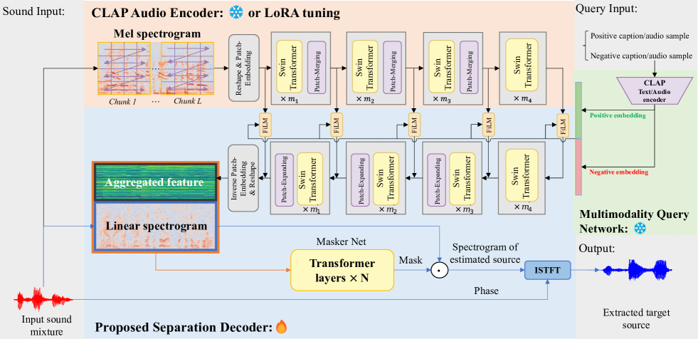
Figure 3: Overview of proposed CLAPSep model.

III Problem Formulation and Proposed Approach

III-A Problem Formulation

To provide a formal definition of the TSE problem, we begin with the definition of the involved symbols. The sound mixture $\tilde{\mathbf{x}}\in\mathbb{R}^{N}$ of length $N$, comprising multiple sound sources, can be expressed as the sum of the target sound source $\mathbf{x}\in\mathbb{R}^{N}$ and other interfering components $\mathbf{v}\in\mathbb{R}^{N}$,

$$\tilde{\mathbf{x}}=\mathbf{x}+\mathbf{v}$$ (1)

The objective is to extract the target sound source $\mathbf{x}$ from other interfering components in $\tilde{\mathbf{x}}$ using the target source’s cues,

$$\hat{\mathbf{x}}=\mathcal{F}(\tilde{\mathbf{x}},\mathbf{c};\theta_{\mathcal{F}})$$ (2)

where $\hat{\mathbf{x}}$ represents the target sound source predicted by a neural network $\mathcal{F}$, which is parameterised by $\theta_{\mathcal{F}}$. The condition embedding $\mathbf{c}\in\mathbb{R}^{D}$ is utilized to guide $\mathcal{F}$ and is extracted by encoding multi-modal user queries.

III-B Proposed CLAPSep Model

The proposed CLAPSep model extracts the target sound from a sound mixture conditioned on a series of user-specified queries. These queries are multi-modal, allowing for both text and audio modalities, and can include positive and/or negative samples to guide the extraction process. The CLAPSep is comprised of three components: a query network, an audio encoder, and a separation decoder. The query network encodes the user-specified queries into positive-negative embedding pairs. The audio encoder extracts multi-level fine-grained features from the sound mixture. The separation decoder estimates the spectrogram of the target sound conditioned on the encoded audio feature and the query embedding pairs. Finally, the target sound can be reconstructed from the estimated spectrogram and the phase of the input sound mixture. In the following section, we will give a detailed description of the three components.

III-B1 Query Network

The query network transforms user queries (text and/or audio) into condition embeddings. We leverage the text and audio encoders of the contrastive language audio pre-trained (CLAP) model, which brings audio and text descriptions into a joint multi-modal space. All parameters of the query network are frozen in training the proposed CLAPSep model. Formally, consider a user query with text and audio, denoted by ${\bm{q}}_{\text{text}}$ and ${\bm{q}}_{\text{audio}}$. CLAP transforms them into embeddings ${\bm{e}}_{\text{text}}$ and ${\bm{e}}_{\text{audio}}$ in the same $D$-dimensional space, ${\bm{e}}_{\text{text}},{\bm{e}}_{\text{audio}}\in\mathbb{R}^{D}$. The stochastic linear interpolation [24] is applied as a multi-modal training strategy to mitigate the modality gap between text and audio condition embeddings, facilitating multi-modality querying capability,

$${\bm{e}}=\alpha{\bm{e}}_{\text{audio}}+(1-\alpha){\bm{e}}_{\text{text}},$$ (3)

where $\alpha$ is randomly sampled from a uniform distribution $U(0,1)$. In testing, $\alpha$ is set to 0, 1, and 0.5 for text-only, audio-only, and text-audio user queries, respectively. Eq.3 is applied to the user’s positive and negative queries separately, producing embeddings ${\bm{e}}^{P}$ and ${\bm{e}}^{N}$. Finally, the two embeddings are concatenated as the output, namely the condition embedding ${\bm{c}}=[{\bm{e}}^{P},{\bm{e}}^{N}]$. When the positive or negative query is missing, we zero the corresponding embedding, e.g., ${\bm{c}}=[\mathbf{0},{\bm{e}}^{N}]$ or $[{\bm{e}}^{P},\mathbf{0}]$.

In training, positive-only, negative-only, and positive-negative queries are constructed with proportions of $0.25,0.25$ and $0.5$.

III-B2 Audio Encoder

The pre-trained CLAP audio encoder is leveraged to extract multi-level features from the input sound mixture. Parameters of the audio encoder are partially tuned by LoRA [30] in training. The audio encoder follows the structure of HTSAT [31], which is an $L$-layer cascaded swin-transformer [32]. As shown in Fig. 3, it takes the Mel-spectrogram $\tilde{|\mathbf{X}}|_{Mel}\in\mathbb{R}^{T\times F}$ of the sound mixture $\tilde{\mathbf{x}}$ as input, which is consistent with the input form of the pre-trained CLAP model. $T$ and $F$ denote the number of time frames and frequency bins, respectively. $\tilde{|\mathbf{X}}|_{Mel}$ is first reshaped to patch sequence. Specifically, The Mel-spectrogram is split into chunks, and then patches are split inside each chunk with stride $P$. To better capture the time-frequency relationship between T-F bins, these patches are then reordered into patch sequence following time→frequency→chunk as shown in Fig. 3. Then, the reordered patch sequence is fed into a patch embedding layer to get the first-level audio feature $\mathbf{H}_{e}^{0}$ as:

$$\mathbf{H}_{e}^{0}=\mathrm{PatchEmbed}(\mathrm{Reshape}(|\tilde{\mathbf{X}}|_{Mel})),$$ (4)

where $\mathbf{H}_{e}^{0}$ has the shape $({\frac{T}{P}\times\frac{F}{P}},D_{f})$, where $D_{f}$ is the feature dimension. $\mathbf{H}_{e}^{0}$ is then processed by the $L$ layers of swin-transformer to extract layer-wise audio features,

$$\mathbf{H}_{e}^{l}={f}_{enc}^{l}(\mathbf{H}_{e}^{l-1}),$$ (5)

where ${f}_{enc}^{l}(\cdot)$ denotes the $l$-th encoder layer, with a patch-merging module halving the feature map’s width and height and doubling the feature dimension.

III-B3 Separation Decoder

Given the condition embedding ${\bm{c}}$ and the multi-level audio features $\{\mathbf{H}_{e}^{l}\}_{l=1}^{L}$, a separation decoder is employed to separate the target sound ${\bm{x}}$ from the sound mixture. The separation decoder consists of two components: a feature aggregator and a MaskNet.

To begin with, a STFT module is used to extract magnitude and phase spectrogram of the input sound mixture as:

$$\tilde{\mathbf{X}}=\mathrm{STFT}(\tilde{{\bm{x}}})=|\tilde{\mathbf{X}}|e^{j\mathbf{\Phi}_{\tilde{\mathbf{X}}}},$$ (6)

where $\tilde{\mathbf{X}}$ denotes the complex spectrogram, and $|\tilde{\mathbf{X}}|$, $\mathbf{\Phi}_{\tilde{\mathbf{X}}}$ denote magnitude and phase spectrogram, respectively. $j$ is the imaginary unit.

The feature aggregator follows the U-Net structure, extracting target sound features by hierarchically aggregating the layer-wise audio features and the condition embedding. More specifically, the layer-wise audio features $\mathcal{H}_{e}$ are firstly element-wisely linear modulated (FiLM) [33] by the condition embedding ${\bm{c}}$ as:

$${\mathbf{H}_{c}^{l}}=\gamma_{l}(\mathbf{c})\mathbf{H}_{e}^{l}+\beta_{l}(\mathbf{c}),$$ (7)

where $\gamma_{l}(\cdot)$ and $\beta_{l}(\cdot)$ can be arbitrary functions. In this work, we parameterize them as two linear layers. Then, the modulated features are fed into the aggregator through skip-connection [34] and aggregated hierarchically as:

$$\begin{split}\mathbf{H}_{d}^{1}={f}_{aggr}^{1}({\mathbf{H}_{c}^{L}})+{\mathbf{H}_{c}^{L-1}},\\ \mathbf{H}_{d}^{l}={f}_{aggr}^{l}({\mathbf{H}_{d}^{l-1}})+{\mathbf{H}_{c}^{L-l}},\\ \end{split}$$ (8)

where $\mathbf{H}_{d}^{l}$ denotes the hidden feature extracted form the $l$-th aggregator layer ${f}_{aggr}^{l}(\cdot)$. Each of the last three aggregator layers is followed by a patch-expanding module. This module serves to augment the number of tokens/patches while reducing their dimensions, thereby aligning their shapes with those of the encoded multi-level audio features. Ultimately, the hidden feature $\mathbf{H}_{d}^{L}$ undergoes an inverse patch-embedding process. This involves a transpose convolution operation, succeeded by a reshape operation that functions inversely to the one detailed in III-B2, consequently yielding the aggregated target source feature.

$$\mathbf{H}_{d}=\mathrm{Reshape^{\prime}}(\mathrm{InversePatchEmbed}(\mathbf{H}_{d}^{L})).$$ (9)

In this way, the aggregated feature $\mathbf{H}_{d}$ is considered to include rich information about the target sound.

Then a $N$-layer transformer-based MaskNet takes the concatenation of the aggregated feature $\mathbf{H}_{d}$ and linear magnitude spectrogram $|\tilde{\mathbf{X}}|$ of the sound mixture to generate a spectrogram mask, which is activated by Sigmoid activation that constrains the mask value to $(0,1)$:

$$\mathbf{M}=Sigmoid(\mathrm{MaskNet}(\mathrm{Concat}(\mathbf{H}_{d},|\tilde{\mathbf{X}}|))).$$ (10)

Finally, we use inverse short-time Fourier transformation (ISTFT) to get the extracted sound source waveform:

$$\mathbf{\hat{x}}=\mathrm{ISTFT}(\mathbf{M}\odot|\tilde{\mathbf{X}}|e^{j\mathbf{\Phi}_{\tilde{\mathbf{X}}}}),$$ (11)

where $\odot$ denotes element-wise production. To execute inverse short-time Fourier transform (ISTFT), we employ the phase of the sound mixture $\mathbf{\Phi}_{\tilde{\mathbf{X}}}$ as an estimation for the phase of the extracted sound source.

III-B4 LoRA Tuning

Low-rank adaptation (LoRA) [30] was first proposed in NLP as a parameter-efficient fine-tuning (PEFT) paradigm to adapt pre-trained large language models (LLMs) for new downstream tasks. When fine-tuning a pre-trained model with LoRA, all the weights of the pre-trained model keep fixed and only low-rank incremental weight matrices of the model weights are updated. Specifically, for a linear layer of weight $\mathbf{W}_{0}\in\mathbb{R}^{d\times k}$ that perform linear projection of input features as:

$$\mathbf{h}^{{}^{\prime}}=\mathbf{W}_{0}\mathbf{h}.$$ (12)

When fine-tuning the linear layer, we are learning an incremental matrix $\Delta\mathbf{W}$ as:

$$\mathbf{h}^{{}^{\prime}}=(\mathbf{W}_{0}+\Delta\mathbf{W})\mathbf{h}.$$ (13)

In LoRA, the incremental matrix is represented as a low-rank decomposition $\mathbf{W}_{0}+\Delta\mathbf{W}=\mathbf{W}_{0}+\mathbf{B}\mathbf{A}$, where $\mathbf{B}\in\mathbb{R}^{d\times r}$, $\mathbf{A}\in\mathbb{R}^{r\times k}$ and $r\ll min(d,k)$ to ensure low-rank propriety.

The low-rank propriety brings many advantages. It saves a lot of computational costs compared with a full fine-tuning strategy and it can prevent catastrophic forgetting in low-data settings. In our task, we expect the pre-trained CLAP audio encoder to adapt to the TSE task while retaining knowledge about diverse sound classes learned during its pre-training phase, we adopt LoRA tuning for the CLAP audio encoder when training the CLAPSep model.

III-B5 Loss Function

CLAPSep is trained in an end-to-end manner. The training loss is defined as the combination of negative signal-to-distortion ratio (SDR) and negative scale-invariant signal-to-distortion ratio (SISDR) [35],

$$\mathcal{L}(\mathbf{\hat{x}},\mathbf{x})=-\lambda\mathrm{SDR}(\mathbf{\hat{x}},\mathbf{x})-(1-\lambda)\mathrm{SISDR}(\mathbf{\hat{x}},\mathbf{x}),$$ (14)

where

$$\mathrm{SDR}(\mathbf{\hat{x}},\mathbf{x})=10\mathrm{log}_{10}(\frac{||\mathbf{x}||^{2}}{||\mathbf{x}-\mathbf{\hat{x}}||^{2}}),$$ (15)

$$\mathrm{SISDR}(\mathbf{\hat{x}},\mathbf{x})=10\mathrm{log}_{10}(\frac{||\frac{||\mathbf{\hat{x}}^{T}\mathbf{x}||^{2}}{||\mathbf{x}||^{2}}\mathbf{x}||^{2}}{||\frac{||\mathbf{\hat{x}}^{T}\mathbf{x}||^{2}}{||\mathbf{x}||^{2}}\mathbf{x}-\mathbf{\hat{x}}||^{2}}),$$ (16)

where $\mathbf{\hat{x}}$ and $\mathbf{x}$ denote the estimated waveform and the ground truth waveform, respectively. $\lambda$ is set to 0.9 in this work.

IV Experimental Setup

IV-A Datasets

IV-A1 Training Data

We use AudioCaps [36] to craft sound mixtures for model training. AudioCaps is developed for audio captioning, consisting of around 50k audio-text pairs. The pairs are collected via crowdsourcing on AudioSet [37]. The audio clips are sampled at 32kHz and the length of each audio clip is about 10s. We follow the procedure in [20] to create sound mixtures by randomly selecting two audio clips along with their corresponding text captions. Then, we treat one of these two audio clips as the target source and the other as interference noise and mix them at an SNR of 0dB. The text captions of the target source and interference noise are used as positive and negative language queries. Regarding the query audio samples, due to the complexity of the caption annotation of each audio clip, it is difficult to find a semantically consistent but different audio sample to serve as the query audio. Thus, we simply use the target source and interference noise that construct the sound mixture as positive and negative query audio samples. To prevent overfitting, we do augmentations including speed perturbation and time-frequency masking [38] on the query audio samples. All sound mixtures are created on the fly to increase the diversity of training data.

IV-A2 Test Data

We use multiple datasets to perform a comprehensive evaluation of our proposed method. This includes AudioCaps [36], AudioSet [37], ESC-50 [39] and FSDKaggle2018 [40] for universal sound separation and MUSIC21 [18] for musical instrument separation. In each dataset, evaluation sound mixtures are generated by considering each audio clip as a target source. Subsequently, either 1 or 5 additional audio clips are randomly chosen as interference noise. The mixing process involves combining one target source with one interference noise at a signal-to-noise ratio (SNR) of 0dB, resulting in the creation of 1 or 5 evaluation mixtures for each target source. For label-annotated datasets, we transform the labels into language descriptions by adding the prefix “The sound of”. For ESC-50, FSDKaggle2018, and MUSIC21, we also randomly choose 10 audio clips for each sound class as query audio samples to evaluate the multimodality-queried TSE capability of the proposed approach. These selected query samples are not used to generate evaluation mixtures, in order to avoid information leakage. In the following section, we will introduce all the evaluation datasets we used in our experiments.  

AudioCaps. We use the official test split of the AudioCaps dataset to create evaluation sound mixtures. There are a total of 957 audio clips in the official test split. We use these audio clips to create 4,785 evaluation sound mixtures. In the officially releases dataset, each audio clip has 5 annotated audio captions. We use the first caption as a language query.  

AudioSet is a large-scale human-labeled audio collection drawn from YouTube videos. The whole AudioSet corpus comprises 2,084,320 annotated audio clips belonging to 527 sound classes. These class labels cover a wide range of sound events including human speech, instrumental music, environmental sounds among others. All the audio clips are sampled at 32kHz and the length of each audio clip is 10 seconds, amounting to a total of about 5.8k hours. We use the official evaluation split of the whole dataset which contains 20,371 audio clips and we downloaded 18,869 out of the total due to some YouTube links are no longer available to create 18,869 evaluation sound mixtures.

TABLE I: Training data counting

Methods	Training corpus	Num. of clips	Hours
AudioSep [20]	AudioSet+AudioCaps+others	2 342 568	14 100
USS [8]	AudioSet	2 063 839	5 800
Waveformer [13]	FSDKaggle2018	9 500	18
LASS [19]	AudioCaps (subset)	6 244	17
Ours	AudioCaps	49 768	145

TABLE II: Language-queried target sound extraction performance evaluation and SOTA comparison. For compared methods, we run evaluations with the officially released model weights. ^† denotes we re-trained these models with the same training data as CLAPSep. In the query valence column, we use P to denote a positive query and N to denote a negative query.

Methods	Query	Query	AudioCaps		AudioSet		MUSIC21		ESC-50		FSDKaggle2018
	Modality	Valence	SDRi	SISDRi	SDRi	SISDRi	SDRi	SISDRi	SDRi	SISDRi	SDRi	SISDRi
AudioSep [20]	Text	P	7.75±5.59	7.04±5.72	8.02±6.23	7.26±6.44	8.73±7.71	7.84±8.09	10.33±7.61	9.20±7.97	13.90±15.44	11.57±17.72
AudioSep†	Text	P	6.63±5.46	5.55±5.77	3.81±6.64	2.30±7.29	0.98±5.48	0.15±6.04	7.66±7.92	5.81±8.78	7.59±11.45	5.45±12.88
LASS [19]	Text	P	0.33±7.39	-1.11±8.18	-2.57±7.86	-4.41±8.60	-6.63±7.42	-9.83±7.91	-0.48±9.97	-2.60±11.31	-3.89±14.05	-9.70±16.76
LASS†	Text	P	6.75±5.59	6.05±5.86	3.12±7.61	2.02±8.29	-1.70±8.14	-3.62±9.06	7.49±9.06	6.07±10.18	6.55±16.48	3.27±19.35
Waveformer [13]	Label	P	-	-	-	-	-	-	-	-	7.77±11.33	5.68±12.11
CLAPSep-hybrid	Text	P	9.51±5.19	8.81±5.35	7.86±7.18	6.88±7.63	3.62±9.75	1.88±10.97	10.56±9.09	9.23±10.04	16.06±16.89	14.03±19.76
		N	9.55±5.07	8.85±5.19	7.90±7.11	6.99±7.53	4.00±9.25	2.32±10.20	10.14±9.83	8.70±11.13	15.86±17.42	13.69±20.59
		P+N	10.05±4.41	9.40±4.41	9.15±5.71	8.31±5.86	8.40±6.21	7.23±6.36	12.81±6.42	11.74±6.68	20.01±12.48	18.75±13.64
CLAPSep-text	Text	P	9.64±5.09	8.92±5.27	8.02±7.17	7.05±7.60	5.34±9.13	3.78±9.89	12.23±7.52	11.14±8.01	16.92±15.83	15.14±18.25
		N	9.65±5.03	8.94±5.17	7.98±7.21	7.05±7.64	6.24±8.12	4.99±8.70	12.19±7.41	11.12±7.97	16.42±16.88	14.27±19.94
		P+N	10.08±4.42	9.40±4.45	9.29±5.61	8.44±5.75	8.32±6.56	7.10±6.71	13.09±6.22	12.10±6.37	20.17±12.43	18.91±13.38

ESC-50 is a labeled collection of environmental audio clips extracted from public field recordings gathered by the Freesound project [41]. The ESC-50 dataset comprises 2,000 5-second-long audio clips belonging to 50 environmental sound classes such as car horn, and pouring water, among others. Each audio clip is assigned to one class label and all the audio clips are sampled at 44.1kHz. For consistency comparison, we downsample the audio clips to 32kHz. Since there is no official test split, we use the whole dataset to create 6,500 evaluation sound mixtures after filtering 500 audio clips used as query audio samples.  

FSDKaggle2018 consists of 11,073 audio files annotated with 41 labels, covering both natural sounds and instrumental music. All the sound samples are gathered from the Freesound project [41] and sampled at 44.1kHz. We resample the audio clips to 32kHz for consistency. To create evaluation sound mixtures, we use the official test split which contains 1,600 audio clips to create 8,000 evaluation sound mixtures.  

MUSIC21 comprises instrumental music segments drawn from YouTube videos. In this dataset, there are a total of 1,164 videos belonging to 21 instrumental music classes. Due to some YouTube links are no longer available, we are able to get 1,046 videos. After downloading these videos, we split each video into 10-second-long segments and extracted the audio clips from the video segments. All the audio clips are resampled to 32kHz for consistency. After filtering out some silent clips and some clips used as query samples, we finally got 19,805 10-second audio clips in total to create 19,805 sound mixtures for evaluation.

IV-B Implementation Details

To load pre-trained weights of CLAP, we select a checkpoint trained on both a music dataset and the original LAION-Audio-630k [22] dataset, which performs zero-shot classification accuracy of 90.14% on ESC-50. Based on the pre-trained CLAP, we build our CLAPSep model.

To extract a linear spectrogram for a 10-second audio clip sampled at 32kHz, we set the window length to 1024 and the hop length to 320. In each frame, we compute a Fourier transform of 1024 bins, resulting in a magnitude spectrogram of 513 frequency bins and 1001 time frames. The hyperparameters set to extract the Mel spectrogram are consistent with those of the pre-trained CLAP audio encoder, i.e. the input sound mixture is firstly up-sampled to 48kHz, then a linear spectrogram is extracted by setting the window length to 1024 and the hop length to 480 to compute Fourier transform of 1024 bins for 1001 frames. The Mel spectrogram of 64 Mel bins is computed from the linear spectrogram. The hyperparameters corresponding to the model structure in Fig. 3 are set as follows: $[m_{1},m_{2},m_{3},m_{4}]=[2,2,12,2]$, $[{m_{1}^{{}^{\prime}}},{m_{2}^{{}^{\prime}}},{m_{3}^{{}^{\prime}}},{m_{4}^{{}^{\prime}}}]=[1,1,1,1]$ and MaskNet layers $N=3$.

Only the separation decoder and LoRA module applied to the CLAP audio encoder are learnable in training. LoRA is applied to the query, key, value, and output projection layer in all the multi-head attention modules. The rank of LoRA is set to 16. AdamW [42] optimizer is applied with the learning rate decayed from 1e-4 to 5e-6. The learning rate is exponentially decayed with a factor of 0.3 when the validation loss stops decreasing for five consecutive epochs. We set the batch size to 32. The model is trained with brain float 16 mixed precision on one RTX 3090 with 24GB GPU memory for a total of 150 epochs.

IV-C Evaluation Metrics

Following previous works [19, 20], we use signal-to-distortion ratio improvement (SDRi) and scale-invariant signal-to-distortion ratio improvement (SISDRi) as the evaluation metrics. They indicate to what extent SDR and SISDR (defined in equation 15 and equation 16) are improved by sound separation. They are defined as follows,

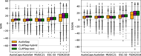
Figure 4: Illustration of SDRi and SISIDRi distributions w.r.t. different language-queried TSE models on 5 evaluation datasets.

$$\mathrm{SDRi}(\mathbf{\hat{x}},\mathbf{\tilde{x}},\mathbf{x})=\mathrm{SDR}(\mathbf{\hat{x}},\mathbf{x})-\mathrm{SDR}(\mathbf{\tilde{x}},\mathbf{x}),$$ (17)

$$\mathrm{SISDRi}(\mathbf{\hat{x}},\mathbf{\tilde{x}},\mathbf{x})=\mathrm{SISDR}(\mathbf{\hat{x}},\mathbf{x})-\mathrm{SISDR}(\mathbf{\tilde{x}},\mathbf{x}),$$ (18)

where $\mathbf{\hat{x}}$, $\mathbf{\tilde{x}}$ and $\mathbf{x}$ denote the extracted sound source, sound mixture, and ground truth source, respectively.

V Results and Analysis

V-A Language-Queried TSE Performance Evaluation

TABLE III: Multimodality-queried target sound extraction performance evaluation and SOTA comparison. For compared methods, we run evaluations with the officially released model weights. Shots denotes the number of 10-second audio clips chosen as query samples.

Methods	Query	Shots	Query	MUSIC21		ESC-50		FSDKaggle2018
	Modality		Valence	SDRi	SISDRi	SDRi	SISDRi	SDRi	SISDRi
USS-ResUNet30 [8]	Audio	1	P	6.96±7.44	6.17±8.01	8.17±7.67	7.08±8.05	9.99±13.04	8.00±15.03
		5		8.06±6.56	7.38±6.84	9.29±6.94	8.38±7.06	12.10±11.15	11.04±11.45
		10		8.32±6.38	7.69±6.61	9.51±6.69	8.68±6.75	12.02±11.16	11.03±11.43
CLAPSep-text	Audio	10	P+N	5.39±5.45	4.36±5.47	6.93±6.57	6.16±6.81	7.79±10.49	6.79±11.09
	Audio+Text	-	P+N	8.36±5.67	7.22±5.69	12.12±6.13	11.17±6.26	19.64±11.56	18.43±12.27
	Audio	1	P	6.34±7.95	5.02±8.51	12.08±7.57	10.88±7.99	15.41±17.52	13.01±20.86
			N	6.33±8.23	4.93±8.76	11.76±7.75	10.80±8.29	15.21±17.89	13.23±20.60
			P+N	8.41±6.34	7.21±6.50	12.89±6.41	11.94±6.53	19.04±13.53	17.64±14.93
		5	P	6.75±7.91	5.41±8.43	12.72±6.67	11.65±6.83	17.77±15.18	15.84±17.70
			N	6.77±8.00	5.42±8.53	12.49±6.78	11.61±6.97	17.56±15.36	16.01±17.37
CLAPSep-hybrid			P+N	9.07±5.88	7.86±6.00	13.26±6.10	12.34±6.14	20.12±12.12	18.91±13.01
		10	P	6.98±7.72	5.67±8.19	12.79±6.63	11.73±6.78	17.97±14.88	16.15±17.12
			N	7.05±7.82	5.71±8.29	12.64±6.64	11.75±6.81	17.83±15.06	16.33±16.93
			P+N	9.35±5.59	8.16±5.65	13.29±6.09	12.37±6.13	20.25±11.88	19.07±12.71
	Audio+Text	-	P	6.91±7.92	5.54±8.56	12.46±7.16	11.30±7.47	18.87±14.02	17.28±15.80
			N	7.20±7.72	5.86±8.23	12.28±7.18	11.29±7.66	18.95±13.95	17.54±15.67
			P+N	9.47±5.53	8.26±5.62	13.21±6.16	12.24±6.23	21.11±11.22	20.01±11.84

In this section, we demonstrate the language-queried target sound extraction capabilities of our proposed method through a comparison with other SOTA language-queried target sound extraction models. We choose two SOTA models, namely LASS [19] and AudioSep [20], as baselines and compare our proposed model with them to highlight the effectiveness of our approach. To provide context, let’s begin with a brief introduction to these two baseline models.

LASS is a language-queried target sound extraction model. Similar to our proposed method, it utilizes a natural language description as a query to guide the separation model in performing target sound extraction. The key distinction from our proposed CLAPSep lies in the fact that LASS does not leverage any multi-modal contrastive pre-trained models. Consequently, it is required to train a BERT-based language query network and a separation network simultaneously.

AudioSep is another language-queried target sound extraction model that demonstrates SOTA performance on many benchmarks. As an improvement upon LASS, it incorporates the pre-trained text encoder of a contrastive pre-trained model as a query network. Additionally, AudioSep utilizes a substantially larger amount of training data compared to LASS, resulting in a significant performance advantage across many benchmarks. It is important to note that, in contrast to our proposed CLAPSep model, AudioSep lacks the reuse of the audio encoder from the pre-trained CLAP model.

For the two aforementioned compared methods, we initially conduct evaluations using their officially released model weights. Furthermore, considering that our proposed model is trained on different data compared to these models, as shown in Table I, we meticulously re-implement LASS and AudioSep using our training data to ensure a consistent and fair comparison.

In addition, a SOTA label-queried TSE model called Waveformer [13] is also included for comparison.

All the results are presented in Table II. In addition to the mean values of SDRi and SISDRi, we also include the standard deviation across samples to illustrate the extent of fluctuation in SDRi and SISDRi. A smaller standard deviation implies a more consistent performance for a TSE system.

In the context of our proposed CLAPSep model, we present results for two versions, namely CLAPSep-hybrid and CLAPSep-text, in Table II. CLAPSep-hybrid undergoes training in a multi-modal hybrid manner as outlined in equation 3, while CLAPSep-text is exclusively trained on text queries. Notably, CLAPSep-text exhibits a slightly superior performance compared to CLAPSep-hybrid in language-queried TSE evaluations.

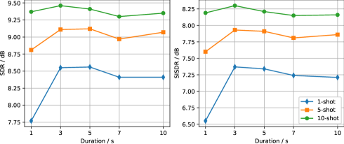
Figure 5: Illustration of SDR and SISDR varying with the number and duration of query audio samples.

Upon analyzing these outcomes, it is evident that the label-queried TSE model Waveformer can only perform TSE on FSDKaggle2018 where the query labels are defined. This limitation highlights a substantial gap in achieving universal sound separation.

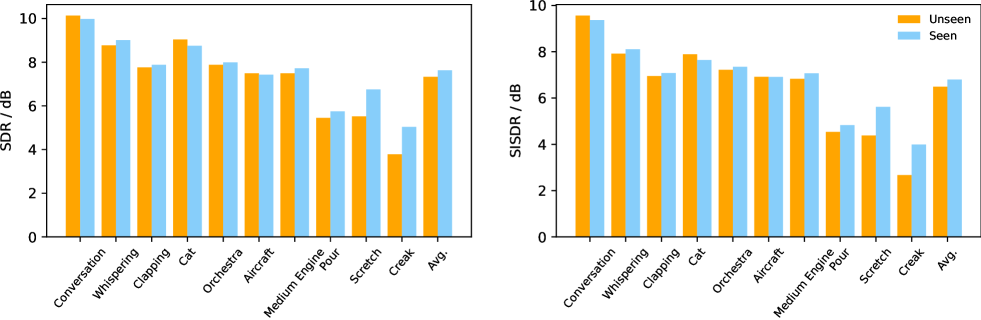
Figure 6: Zero-shot generalizability evaluation. The terms Seen and Unseen indicate evaluation results concerning models encountered or not encountered in these 10 sound event classes during their training phase.

The remaining compared methods are all language-queried TSE models. From the results presented in Table II, it is evident that the original LASS, despite being trained on a smaller dataset as indicated in Table I, fails to exhibit satisfactory performance on these benchmarks. The re-implemented LASS, trained on the same dataset as our CLAPSep, displays a substantial performance improvement, but it still falls significantly short of our proposed method. On the contrary, AudioSep initially trained on a much larger dataset, demonstrates state-of-the-art (SOTA) performance. However, when AudioSep is re-trained on the same data as ours, there is a notable decline in performance, particularly evident in cross-dataset evaluations. This decline underscores that the generalizability of this model is predominantly derived from extensive training on large-scale data.

Further comparing the re-implemented LASS^† and AudioSep^† reveals that, although LASS^† outperforms AudioSep^† on the evaluation split of AudioCaps, where the training split is utilized to train both models, AudioSep^† exhibits superior cross-dataset generalizability. This outcome suggests that reusing the pre-trained CLAP text encoder so as to decouple the training of the query network and the separation network contributes to the generalizability of TSE models.

Turning to our proposed CLAPSep model, it is evident that our model effectively extracts the desired target source by providing only positive queries and suppresses unwanted sounds by providing negative queries alone. The combination of positive and negative queries enables the model to achieve optimal TSE performance. When comparing CLAPSep with the previous SOTA TSE model AudioSep, our proposed method attains new SOTA performances on most evaluation benchmarks, especially when queried with both positive and negative language descriptions. Remarkably, CLAPSep is trained on a considerably smaller dataset compared to AudioSep, highlighting the effectiveness of our model in inheriting prior knowledge embedded in the pre-trained CLAP model.

To provide a more comprehensive comparison, we visualize the SNRi and SISINRi distribution of CLAPSep and the previous SOTA AudioSep on 5 evaluation datasets in Fig. 4. The SNRi/SISNRi obtained using our method is larger in the median and more centrally distributed, indicating superior TSE performance and greater stability.

V-B Multimodality-Queried TSE Performance Evaluation

While our proposed method attains SOTA performance on the majority of benchmarks in language-queried target sound extraction evaluations, it is crucial to acknowledge that this performance is inherently capped by the language modeling capability of the pre-trained CLAP text encoder. To address this limitation, we introduce an approach where query audio samples are provided to the TSE model. These samples instruct the model to separate target sound sources that align semantically with the provided audio samples. Importantly, these audio samples are directly encoded by the CLAP audio encoder, eliminating the impact of the CLAP text encoder’s imperfect language modeling on the overall TSE system performance. For this concern, we conduct experiments to explore the multi-modality TSE performance of our proposed method.

In this section, we introduce another audio-queried TSE model called USS [8] for comparison. It is noteworthy that USS is also trained on a significantly larger scale training dataset compared to our proposed method. The results are presented in Table III, where “Shots” denotes the number of query audio samples chosen for each sound class. When using more than one query audio sample for a sound class, we average the query embeddings extracted from all query audio samples to obtain the final condition embedding.

From Table III, we first observe that the CLAPSep model, when not trained in a multi-modal hybrid manner (denoted as CLAPSep-text), exhibits unsatisfactory performance when queried by audio samples. In contrast, the model trained in a hybrid manner (denoted as CLAPSep-hybrid) demonstrates improved performance in multimodality-queried TSE tasks, affirming the effectiveness of the multimodal training strategy (as indicated in equation 3) in mitigating the modality gap between CLAP audio and text encoders. Compared with previous SOTA USS, our proposed model achieves new SOTA on ESC-50 and FSDKaggle2018 when queried by positive queries only. When negative queries are also available, our model outperforms USS by more than 1 dB on MUSIC21. Further augmenting the query audio embedding with text embedding (referred to as “Audio+Text”), the proposed CLAPSep model achieves the best performance on the majority of evaluation benchmarks. This underscores the effectiveness of our proposed method in multimodality-queried target sound extraction.

Fig. 5 provides further insight into how the number and duration of query audio samples impact a TSE system’s performance. The number of query audio samples, referred to as “Shots,” plays a significant role in audio-queried TSE performance. When audio samples are selected randomly, a higher number of samples offers richer semantic information, thereby enabling a more accurate representation of the sound class. Conversely, the duration of query audio samples exhibits a “sweet spot” effect. Specifically, when the duration of query audio samples reaches 3 seconds, the TSE system demonstrates its optimal performance. This phenomenon occurs because a 3-second clip of query audio adequately captures the common characteristics of a sound event class. Longer durations may include individual characteristics of audio segments that can potentially diminish performance.

V-C Zero-Shot Generalizability Evaluation

TABLE IV: Ablation study of language-queried TSE performance. Both positive and negative queries are used in these experiments. Here, the best model denotes CLAPSep-hybrid, w/o CLAP audio encoder means ablating CLAP audio encoder for extracting multi-level audio features, w/o pre-trained weights means the CLAP audio encoder for extracting multi-level audio features is trained from scratch and w/o LoRA denotes the CLAP audio encoder was not updated during training.

Methods	AudioCaps		AudioSet		MUSIC21		ESC-50		FSDKaggle2018
	SDRi	SISDRi	SDRi	SISDRi	SDRi	SISDRi	SDRi	SISDRi	SDRi	SISDRi
best model	10.05±4.41	9.40±4.41	9.15±5.71	8.31±5.86	8.40±6.21	7.23±6.36	12.81±6.42	11.74±6.68	20.01±12.48	18.75±13.64
w/o CLAP audio enc.	7.49±5.37	6.62±5.48	5.50±6.83	4.40±7.06	4.60±7.26	3.29±7.50	8.10±9.51	6.88±10.16	11.32±15.16	9.60±16.68
w/o pre-trained weights	9.33±4.71	8.58±4.77	7.78±6.26	6.79±6.46	6.20±7.58	4.73±8.00	11.40±7.36	10.21±7.96	15.10±15.22	13.48±17.40
w/o LoRA	9.86±4.47	9.17±4.48	8.80±5.79	7.93±5.95	7.48±6.54	6.23±6.81	12.54±6.54	11.46±6.82	19.59±12.41	18.33±13.32

TABLE V: Ablation study of audio-queried TSE performance. 10 audio clips for each sound class were used as query samples.

Methods	MUSIC21		ESC-50		FSDKaggle2018
	SDRi	SISDRi	SDRi	SISDRi	SDRi	SISDRi
best model	9.35±5.59	8.16±5.65	13.29±6.09	12.37±6.13	20.25±11.88	19.07±12.71
w/o CLAP audio enc.	4.69±7.05	3.39±7.20	10.09±7.66	9.02±7.96	12.83±14.14	11.21±15.57
w/o pre-trained weights	6.81±6.83	5.51±7.02	12.28±6.26	11.34±6.43	16.83±13.83	15.38±15.50
w/o LoRA	8.64±5.76	7.42±5.81	13.08±6.08	12.15±6.14	19.52±12.24	18.34±13.06

In this section, we conduct experiments to assess the zero-shot generalizability of our proposed method for unseen classes. Given the intricate nature of the caption annotations in our original training set AudioCaps, we opt to use the label-annotated AudioSet_balanced_train as the training set for experiments in this section. Following previous work [43], we select 10 sound classes (see Fig. 6) as unseen classes and filter out all audio clips belonging to these 10 classes from the training set. To generate evaluation sound mixtures, for each selected sound class, we randomly choose 50 audio clips in the evaluation set. In total, 500 audio clips are selected to construct evaluation sound mixtures. For these 500 audio clips, each is treated as a target source to generate 5 audio mixtures by randomly selecting another 5 audio clips as interference noises and mixing a target source with an interference noise at an SNR of 0dB. This way, we create 250 sound mixtures for each sound class, resulting in a total of 2,500 sound mixtures for evaluation.

All results are presented in Fig. 6 and denoted as “Unseen”. For comparison, we also train the same model on AudioSet_balanced_train without filtering out any audio clips, serving as a benchmark. The corresponding results are denoted as “Seen” in Fig. 6. To mitigate potential label leakage, only positive queries are used in these evaluations.

Comparing the results concerning “Unseen” and “Seen” evaluations, the performance gap is minimal. These results indicate that our proposed CLAPSep model can effectively generalize to sound event classes that were unseen during its training phase by reusing the pre-trained CLAP audio encoder to inherit the prior knowledge about diverse sound event classes embedded in the pre-trained model.

V-D Ablation Study

In this section, we conduct ablation experiments to assess the impact of designed components. Specifically, to evaluate how the CLAP audio encoder for extracting multi-level audio features impacts the performance, we ablate it and the corresponding results are denoted as w/o CLAP audio enc. in Table IV and V. To further investigate how the prior knowledge (i.e. pre-trained model weights) embedded in the pre-trained CLAP audio encoder affects the overall TSE system’s performance, we randomly initialize and train the CLAP audio encoder for extracting multi-level audio features from scratch while keeping the model structure unchanged. We also evaluate how LoRA tuning affects performance by replacing the LoRA-tuned CLAP audio encoder with a pre-trained and fixed one. All models are trained with the same data for the same steps. Results are presented in Table IV and V.

When ablating the CLAP audio encoder for extracting multi-level audio features (referred to as w/o CLAP audio enc.), a notable decline in TSE performance is observed, which proves the effectiveness of both the hierarchical structure and the prior knowledge embedded in pre-trained weights. Furthermore, substituting the pre-trained CLAP audio encoder with a randomly initialized one (referred to as w/o pre-trained weights) also leads to a notable decline in TSE performance, especially in cross-dataset evaluations. This underscores that a significant contributor to our model’s generalizability lies in the prior knowledge embedded in the pre-trained CLAP, further substantiating the effectiveness of reusing the CLAP audio encoder. When ablating the LoRA module, the TSE system also shows a slight performance decrease. This phenomenon highlights the effectiveness of LoRA tuning in adapting the pre-trained CLAP audio encoder to the target sound extraction task.

We also depict the changes in training set loss and validation set SISNR throughout the training process w/ and w/o the pre-trained weights of CLAP audio encoder in Fig. 7. From this illustration, it can be observed that our proposed model leverages the prior knowledge embedded in the pre-trained weights efficiently, resulting in faster convergence and superior performance.

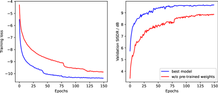
Figure 7: Illustration of training loss and validation SISDRi.

V-E Visualization Analysis

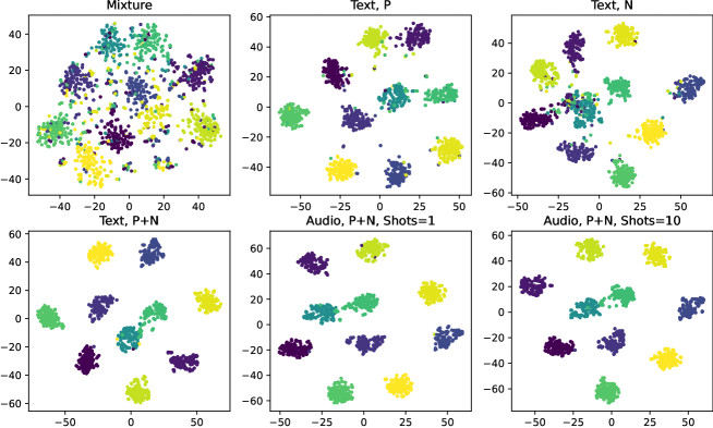
Figure 8: t-SNE visualization of CLAP features derived from mixtures and extracted sources. Points on the scatter plot sharing the same color indicate that these audio sources were queried by the same user query. Text, P denotes the TSE system is queried by positive language description and Audio, P+N, Shots=1 means the system is queried by 1 positive and 1 negative audio samples.

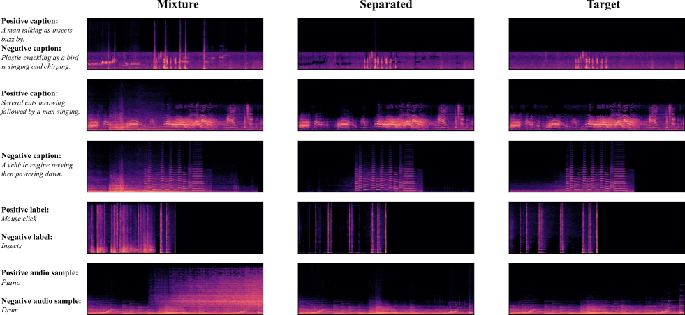
Figure 9: Visualization of spectrograms depicting sound mixtures, separated sources, and ground truth targets.

V-E1 t-SNE Visulization

We begin by conducting t-SNE visualization [44] to further elucidate the capability of the proposed TSE system to handle multi-modal and multi-valance user queries. Specifically, we utilize the pre-trained CLAP audio encoder to compute audio features from the extracted target sources. Subsequently, t-SNE visualization is performed on these CLAP features, and the results are depicted in Fig. 8. Points on the scatter plot sharing the same color indicate that these audio sources were queried by the same user query.

We first present three cases where the model is queried by positive-only, negative-only, and positive-negative user language queries, respectively. From these illustrations, we observe that sound sources extracted through the same user query tend to cluster together, showcasing the effectiveness of the system in target sound extraction and non-target source suppression. Additionally, the clustering of sound sources extracted simultaneously using both positive and negative user queries is more compact, suggesting that richer semantic information enhances the effectiveness of the TSE system.

Fig. 8 also highlights the proposed method’s capability to leverage multi-modal user queries when query audio sample(s) is/are provided.

V-E2 Spectrogram Visulization

In this section, we present visualizations of spectrograms illustrating sound mixtures, separated sources, and ground truth targets. The illustrations are shown in Fig. 9. The first row displays spectrograms of mixtures and extracted target sources queried by AudioCap captions. Notably, even though the model is trained on mixtures of two audio clips, it is capable of extracting multiple sound sources (e.g., man talking and insects buzz) described in the query language at the same time.

The model’s proficiency in target sound extraction and non-target sound suppression is evident in the second and third rows, where positive and negative query captions are the sole inputs. It is evident that the model can effectively extract target sound sources or suppress non-target sound sources when only a positive or negative user query is provided.

The fourth and fifth rows highlight environmental sound extraction queried by labels (which are transformed to language descriptions by adding the prefix “The sound of”) and instrumental music extraction queried by audio samples. A comparison of the spectrograms for sound mixtures, separated sources, and ground truth reveals that our model adeptly preserves the desired sound sources while efficiently eliminating unwanted ones. This demonstrates the effective handling of multimodality-queried target sound extraction tasks by our proposed CLAPSep model.

We also give more audio samples (both synthesis and real-world recordings) on our demo page.

VI Discussion and Conclusion

In this research, we addressed the challenging task of target sound extraction, aiming to extract desired and suppress unwanted sound sources from real-world multi-sources sound mixtures conditioned on multi-modal user queries. While existing approaches often require training models from scratch, our novel strategy leverages the prior knowledge embedded in pre-trained models. Specifically, we built the CLAPSep upon the contrastive language-audio pre-trained model, achieving query-conditioned TSE in a data and computationally efficient way.

Our contributions encompass achieving efficient TSE performance by inheriting capabilities from the pre-trained CLAP model; introducing a multi-modal training strategy that makes the proposed model capable of handling both language queries and audio query samples; incorporating negative queries for sound suppression, significantly enhancing the model’s performance in both target sound extraction and non-target sound suppression.

Extensive evaluations across multiple benchmarks showcase that our approach achieves state-of-the-art TSE performance. Furthermore, our model demonstrates robust generalizability, as evidenced by zero-shot experiments with unseen sound classes.

Although our proposed method contributes to queried-conditioned target sound extraction, there are specific constraints that need further consideration. Firstly, our proposed CLAPSep is not causal, meaning that the separation results at the current time step are influenced by subsequent content. This limitation makes it incapable of real-time streaming TSE applications. Additionally, our approach utilizes the phase of the sound mixture as the phase estimate for the target sound source during ISTFT. In future work, further performance improvements could be achieved by incorporating neural networks to estimate phase residuals.

In summary, our work presents a pioneering approach in query-conditioned target sound extraction, offering a versatile and efficient solution for real-world applications. The integration of pre-trained models, innovative query strategies, and multi-modal training marks a significant advancement in the pursuit of universal sound separation. The availability of our code and pre-trained model also serves as a valuable resource for the research community.

References

- [1] D. Wang and J. Chen, “Supervised speech separation based on deep learning: An overview,” IEEE/ACM Trans. Audio, Speech, Lang. Process., vol. 26, no. 10, pp. 1702–1726, 2018.
- [2] A. Pandey and D. Wang, “Dense cnn with self-attention for time-domain speech enhancement,” IEEE/ACM Trans. Audio, Speech, Lang. Process., vol. 29, pp. 1270–1279, 2021.
- [3] Z. Rafii, A. Liutkus, F.-R. Stöter, S. I. Mimilakis, D. FitzGerald, and B. Pardo, “An overview of lead and accompaniment separation in music,” IEEE/ACM Trans. Audio, Speech, Lang. Process., vol. 26, no. 8, pp. 1307–1335, 2018.
- [4] Y. Luo and N. Mesgarani, “Conv-tasnet: Surpassing ideal time–frequency magnitude masking for speech separation,” IEEE/ACM Trans. Audio, Speech, Lang. Process., vol. 27, no. 8, pp. 1256–1266, 2019.
- [5] C. Macartney and T. Weyde, “Improved speech enhancement with the wave-u-net,” arXiv preprint arXiv:1811.11307, 2018.
- [6] Y. Luo and J. Yu, “Music source separation with band-split rnn,” IEEE/ACM Trans. Audio, Speech, Lang. Process., vol. 31, pp. 1893–1901, 2023.
- [7] Q. Kong, Y. Cao, H. Liu, K. Choi, and Y. Wang, “Decoupling magnitude and phase estimation with deep resunet for music source separation,” arXiv preprint arXiv:2109.05418, 2021.
- [8] Q. Kong, K. Chen, H. Liu, X. Du, T. Berg-Kirkpatrick, S. Dubnov, and M. D. Plumbley, “Universal source separation with weakly labelled data,” arXiv preprint arXiv:2305.07447, 2023.
- [9] I. Kavalerov, S. Wisdom, H. Erdogan, B. Patton, K. Wilson, J. Le Roux, and J. R. Hershey, “Universal sound separation,” in IEEE Workshop on Appl. Signal Process. Audio Acoust. (WASPAA), 2019, pp. 175–179.
- [10] S. Wisdom, E. Tzinis, H. Erdogan, R. Weiss, K. Wilson, and J. Hershey, “Unsupervised sound separation using mixture invariant training,” Proc. Adv. Neural Inf. Process. Syst. (NeurIPS), vol. 33, pp. 3846–3857, 2020.
- [11] Y. Liu, X. Liu, Y. Zhao, Y. Wang, R. Xia, P. Tain, and Y. Wang, “Audio prompt tuning for universal sound separation,” arXiv preprint arXiv:2311.18399, 2023.
- [12] T. Ochiai, M. Delcroix, Y. Koizumi, H. Ito, K. Kinoshita, and S. Araki, “Listen to What You Want: Neural Network-Based Universal Sound Selector,” in Proc. INTERSPEECH, 2020, pp. 1441–1445.
- [13] B. Veluri, J. Chan, M. Itani, T. Chen, T. Yoshioka, and S. Gollakota, “Real-time target sound extraction,” in Proc. Int. Conf. Acoustics Speech Signal Process. (ICASSP), 2023, pp. 1–5.
- [14] M. Delcroix, J. B. Vázquez, T. Ochiai, K. Kinoshita, Y. Ohishi, and S. Araki, “Soundbeam: Target sound extraction conditioned on sound-class labels and enrollment clues for increased performance and continuous learning,” IEEE/ACM Trans. Audio, Speech, Lang. Process., vol. 31, pp. 121–136, 2023.
- [15] K. Kilgour, B. Gfeller, Q. Huang, A. Jansen, S. Wisdom, and M. Tagliasacchi, “Text-Driven Separation of Arbitrary Sounds,” in Proc. INTERSPEECH, 2022, pp. 5403–5407.
- [16] K. Chen*, X. Du*, B. Zhu, Z. Ma, T. Berg-Kirkpatrick, and S. Dubnov, “Zero-shot audio source separation via query-based learning from weakly-labeled data,” in Proc. AAAI Conf. Artif. Intell., 2022.
- [17] H.-W. Dong, N. Takahashi, Y. Mitsufuji, J. McAuley, and T. Berg-Kirkpatrick, “Clipsep: Learning text-queried sound separation with noisy unlabeled videos,” in Proc. Proc. Int. Conf. Learn. Represent. (ICLR), 2023.
- [18] H. Zhao, C. Gan, A. Rouditchenko, C. Vondrick, J. McDermott, and A. Torralba, “The sound of pixels,” in Proc. Eur. Conf. Comput. Vis. (ECCV), September 2018.
- [19] X. Liu, H. Liu, Q. Kong, X. Mei, J. Zhao, Q. Huang, M. D. Plumbley, and W. Wang, “Separate What You Describe: Language-Queried Audio Source Separation,” in Proc. INTERSPEECH, 2022, pp. 1801–1805.
- [20] X. Liu, Q. Kong, Y. Zhao, H. Liu, Y. Yuan, Y. Liu, R. Xia, Y. Wang, M. D. Plumbley, and W. Wang, “Separate anything you describe,” arXiv preprint arXiv:2308.05037, 2023.
- [21] J. Devlin, M.-W. Chang, K. Lee, and K. Toutanova, “Bert: Pre-training of deep bidirectional transformers for language understanding,” arXiv preprint arXiv:1810.04805, 2018.
- [22] Y. Wu, K. Chen, T. Zhang, Y. Hui, T. Berg-Kirkpatrick, and S. Dubnov, “Large-scale contrastive language-audio pretraining with feature fusion and keyword-to-caption augmentation,” in Proc. Int. Conf. Acoustics Speech Signal Process. (ICASSP), 2023.
- [23] A. Radford, J. W. Kim, C. Hallacy, A. Ramesh, G. Goh, S. Agarwal, G. Sastry, A. Askell, P. Mishkin, J. Clark et al., “Learning transferable visual models from natural language supervision,” in Proc. Int. Conf. Mach. Learn. (ICML). PMLR, 2021, pp. 8748–8763.
- [24] T. Lüddecke and A. Ecker, “Image segmentation using text and image prompts,” in Proc. IEEE/CVF Conf. Comput. Vis. Pattern Recognit. (CVPR), 2022, pp. 7086–7096.
- [25] Y. Rao, W. Zhao, G. Chen, Y. Tang, Z. Zhu, G. Huang, J. Zhou, and J. Lu, “Denseclip: Language-guided dense prediction with context-aware prompting,” in Proc. IEEE/CVF Conf. Comput. Vis. Pattern Recognit. (CVPR), 2022, pp. 18 082–18 091.
- [26] C. Zhou, C. C. Loy, and B. Dai, “Extract free dense labels from clip,” in Proc. Eur. Conf. Comput. Vis. (ECCV), 2022.
- [27] A. Vaswani, N. Shazeer, N. Parmar, J. Uszkoreit, L. Jones, A. N. Gomez, Ł. Kaiser, and I. Polosukhin, “Attention is all you need,” Proc. Adv. Neural Inf. Process. Syst. (NeurIPS), vol. 30, 2017.
- [28] C. Subakan, M. Ravanelli, S. Cornell, M. Bronzi, and J. Zhong, “Attention is all you need in speech separation,” in Proc. Int. Conf. Acoustics Speech Signal Process. (ICASSP). IEEE, 2021, pp. 21–25.
- [29] D. Yu, M. Kolbæk, Z.-H. Tan, and J. Jensen, “Permutation invariant training of deep models for speaker-independent multi-talker speech separation,” in Proc. Int. Conf. Acoustics Speech Signal Process. (ICASSP). IEEE, 2017, pp. 241–245.
- [30] E. J. Hu, Y. Shen, P. Wallis, Z. Allen-Zhu, Y. Li, S. Wang, L. Wang, and W. Chen, “Lora: Low-rank adaptation of large language models,” arXiv preprint arXiv:2106.09685, 2021.
- [31] K. Chen, X. Du, B. Zhu, Z. Ma, T. Berg-Kirkpatrick, and S. Dubnov, “Hts-at: A hierarchical token-semantic audio transformer for sound classification and detection,” in Proc. Int. Conf. Acoustics Speech Signal Process. (ICASSP), 2022.
- [32] Z. Liu, Y. Lin, Y. Cao, H. Hu, Y. Wei, Z. Zhang, S. Lin, and B. Guo, “Swin transformer: Hierarchical vision transformer using shifted windows,” in Proc. IEEE/CVF Int. Conf. Comput. Vis. (ICCV), 2021.
- [33] E. Perez, F. Strub, H. De Vries, V. Dumoulin, and A. Courville, “Film: Visual reasoning with a general conditioning layer,” in Proc. AAAI Conf. Artif. Intell., vol. 32, no. 1, 2018.
- [34] O. Ronneberger, P. Fischer, and T. Brox, “U-net: Convolutional networks for biomedical image segmentation,” in Medical Image Computing and Computer-Assisted Intervention–MICCAI 2015: 18th International Conference, Munich, Germany, October 5-9, 2015, Proceedings, Part III 18. Springer, 2015, pp. 234–241.
- [35] J. L. Roux, S. Wisdom, H. Erdogan, and J. R. Hershey, “Sdr – half-baked or well done?” in Proc. Int. Conf. Acoustics Speech Signal Process. (ICASSP), 2019, pp. 626–630.
- [36] C. D. Kim, B. Kim, H. Lee, and G. Kim, “Audiocaps: Generating captions for audios in the wild,” in NAACL-HLT, 2019.
- [37] J. F. Gemmeke, D. P. W. Ellis, D. Freedman, A. Jansen, W. Lawrence, R. C. Moore, M. Plakal, and M. Ritter, “Audio set: An ontology and human-labeled dataset for audio events,” in Proc. Int. Conf. Acoustics Speech Signal Process. (ICASSP), New Orleans, LA, 2017.
- [38] D. S. Park, W. Chan, Y. Zhang, C.-C. Chiu, B. Zoph, E. D. Cubuk, and Q. V. Le, “Specaugment: A simple data augmentation method for automatic speech recognition,” arXiv preprint arXiv:1904.08779, 2019.
- [39] K. J. Piczak, “ESC: Dataset for Environmental Sound Classification,” in Proc. 23rd ACM Conf. Multimedia (ACM-MM). ACM Press, pp. 1015–1018. [Online]. Available: http://dl.acm.org/citation.cfm?doid=2733373.2806390
- [40] E. Fonseca, M. Plakal, F. Font, D. Ellis, X. Favory, J. Pons, and X. Serra, “General-purpose tagging of freesound audio with audioset labels: Task description, dataset and baseline,” in Proc. Detect. Classif. Acoust. Scenes Events (DCASE), 2018.
- [41] F. Font, G. Roma, and X. Serra, “Freesound technical demo,” in Proc. 21st ACM Int. Conf. Multimedia (ACM-MM), 2013, pp. 411–412.
- [42] I. Loshchilov and F. Hutter, “Decoupled weight decay regularization,” arXiv preprint arXiv:1711.05101, 2017.
- [43] K. Chen*, X. Du*, B. Zhu, Z. Ma, T. Berg-Kirkpatrick, and S. Dubnov, “Zero-shot audio source separation via query-based learning from weakly-labeled data,” in Proc. AAAI Conf. Artif. Intell., 2022.
- [44] L. Van der Maaten and G. Hinton, “Visualizing data using t-sne.” J. mach. learn. res., vol. 9, no. 11, 2008.